
Abstract
In paired experiments, participants are grouped into pairs with similar characteristics, and one observation from each pair is randomly assigned to treatment. The resulting treatment and control groups should be well-balanced; however, there may still be small chance imbalances. Building on work for completely randomized experiments, we propose a design-based method to adjust for covariate imbalances in paired experiments. We leave out each pair and impute its potential outcomes using any prediction algorithm such as lasso or random forests. This method addresses a unique trade-off that exists for paired experiments. By addressing this trade-off, the method has the potential to improve precision over existing methods.
1. Introduction
In randomized controlled trials, we expect the pretreatment covariates of the treatment and control groups to be similar except for the treatment itself. However, there will often be small imbalances in baseline covariates due to chance variation in treatment assignment, which can be addressed in multiple ways. One way to improve the precision of the treatment effect estimate would be to adjust for these imbalances during the analysis. Alternatively, it might be possible to balance covariates through the design of the experiment. For example, in paired experiments, participants are organized into pairs prior to treatment assignment, and then, one participant in each pair is randomly assigned to treatment. Ideally, the two participants in each pair would be as similar as possible.
Paired designs are commonly used when the sample size is small. For example, Pane et al. (2014) discuss a randomized trial involving schools in Texas testing the effectiveness of a computer program, the Cognitive Tutor Algebra 1 curriculum. In this trial, schools were organized into 22 pairs and then pair randomized.
While a paired design is often effective at balancing covariates between the treatment and control groups, it may still be helpful to make adjustments for remaining covariate imbalances. Similar situations can occur with other study designs; for example, covariate adjustments may be helpful in rerandomized trials (see Li & Ding, 2020). Perhaps in part because covariate balance is addressed through experimental design, covariate adjustment methods in paired experiments are relatively understudied. Covariate adjustment methods can be model-based or design-based (for a discussion, see Imai et al., 2009; Imbens, 2010). Model-based estimators have the potential to improve efficiency; however, incorrect modeling assumptions can result in bias and increased mean squared error. Design-based estimators rely only on randomization as the basis for inference, diminishing the concern of model misspecification. Hierarchical linear models (see Raudenbush & Bryk, 2002; Woltman et al., 2012) are an example of a model-based approach for blocked experiments including paired experiments. Pinheiro and Bates (2000) and Dixon (2016) note that hierarchical linear models are a common way to analyze blocked experiments. However, the use of such models requires one to make various modeling decisions, potentially raising concerns about model misspecification. For example, Dixon (2016) notes that there is some debate as to whether block effects should be modeled as fixed or random.
As noted above, covariate adjustments in paired experiments are relatively understudied, and design-based methods are even more so. Imbens and Rubin (2015) and Fogarty (2018) discuss regression-based adjustments. Imbens and Rubin work under a superpopulation model, assuming that the pairs within the experiment are drawn at random from an infinite population, and focus on the population average treatment effect. Fogarty examines the use of regression adjustments in paired experiments under a design-based framework, building on the work of Freedman (2008) and Lin (2013), who discuss regression adjustments in completely randomized experiments. More recently, covariate adjustment methods have been proposed for completely randomized and Bernoulli randomized experiments that involve the use of sample splitting and machine learning methods to impute potential outcomes. These include Aronow and Middleton (2013), Wager et al. (2016), Chernozhukov et al. (2018), E. Wu and Gagnon-Bartsch (2018), Spiess (2018), and Rothe (2018). Some of these methods can be used in more general designs including blocked experiments, for example, Aronow and Middleton (2013). However, unlike the case of regression adjustments, there is not currently an analogue to these methods which is specifically for paired experiments.
In this article, we present an analogous approach to these machine learning methods for paired experiments. The method is design-based; however, it also allows for the use of models to improve performance. We leave out each pair and impute the potential outcomes using information from the remaining observations. This imputation can be done with any prediction method such as linear regression or random forests. Regardless of the imputation method, the resulting treatment effect estimate is unbiased and randomization is the basis for inference. This flexibility has several advantages. For example, one issue when making covariate adjustments is choosing which and how many covariates to use. We can address this issue by choosing an imputation method that allows for automatic variable selection. An alternative approach is to use targeted maximum likelihood estimation, which Moore and van der Laan (2009) note allows for automatic variable selection when making covariate adjustments. Balzer, Laan, et al. (2016) and Balzer, Petersen, et al. (2016) propose the use of targeted maximum likelihood estimation in paired experiments.
Our method also addresses an issue that is specific to paired experiments, which we will call the pair inclusion trade-off. In paired experiments, the performance of a covariate adjustment method can suffer if it fails to properly account for the pair assignments. If the relationship between the covariates and outcome within pairs is the opposite of the relationship overall, that is, a Simpson’s paradox occurs, then omitting the pair assignments will hurt precision relative to the unadjusted estimator. However, in cases where the pair assignments are not predictive of the outcome, it is better to ignore the pairing. Both Aronow and Middleton (2013) and E. Wu and Gagnon-Bartsch (2018) present versions of their methods that allow for block randomizations; however, neither of these methods directly address the pair inclusion trade-off. We discuss the pair inclusion trade-off further in Section 4. The framework we present allows us to address the trade-off. We impute two sets of potential outcomes, one in which we account for and the other where we ignore the pair assignments. Having two sets of imputed potential outcomes, we then interpolate between them by minimizing the cross-validated mean squared error. By addressing this trade-off, we protect against the Simpson’s paradox but retain the potential for improvements in precision if the pairing is not informative.
Covariate adjustment methods have also been proposed for matched-pair cluster randomized trials. For example, Small, Ten Have, and Rosenbaum (2008) propose a design-based estimator, while Z. Wu et al. (2014) propose a method that assumes a superpopulation.
This article is organized as follows. In Section 2, we discuss the model and introduce notation. In Section 3, we present the estimator and derive a variance estimate. We discuss the pair inclusion trade-off further and present an imputation method to address it in Section 4. In Section 5, we apply the estimator to simulated data. In Section 6, we use the method to estimate the effect of the Cognitive Tutor Algebra 1 curriculum mentioned above. Section 7 concludes.
2. Background and Notation
2.1. Estimating the Average Treatment Effect
In this article, we work under the Neyman–Rubin model (see Rubin, 1974; Splawa-Neyman et al., 1990), a nonparametric model that is often used to analyze randomized experiments. Consider a randomized experiment in which there are
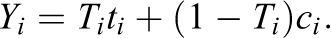
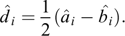
We define the individual treatment effect for each participant as
We first consider a case where the treatment assignments are not pair randomized. Suppose the Ti
are independent Bernoulli random variables with probability

where
2.2. Notation for Paired Experiments
We now consider the case where the participants are pair randomized. Suppose that the
For each pair, one of the two participants is randomly chosen to be assigned to treatment and the other is assigned to control. That is,
When treating each pair as a unit, we can draw direct analogues between the notation of paired and Bernoulli randomized experiments. We denote each pair’s treatment assignment by Ti
, where

We define the pair-level treatment effect

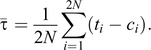
and the average treatment effect

which is our primary parameter of interest.
We can obtain an unbiased estimate for the average treatment effect in paired experiments by averaging the observed differences

We will refer to this estimator as the simple difference estimator for paired experiments, as it is exactly equal to the difference in means between the treatment and control groups. However, the variance estimation of the simple difference estimator will be different under a paired design than it is in completely or Bernoulli randomized experiments. For more details, see Imai (2008), who analyzes
As in the case of completely or Bernoulli randomized experiments, it may be possible to use covariates to improve precision over the simple difference estimator. We propose such a covariate adjustment method for paired experiments in the next section.
3. A Design-Based Covariate Adjustment Procedure
3.1. Estimating the Average Treatment Effect
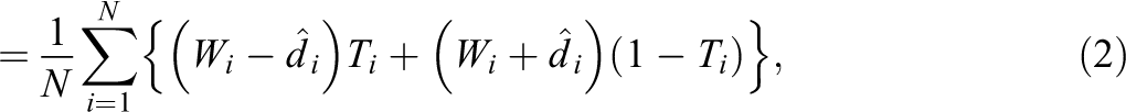
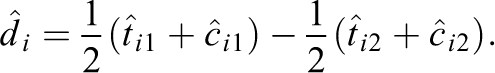
We now present an estimator that is analogous to the estimator given in Equation (1) but for paired experiments. Define the quantity

where
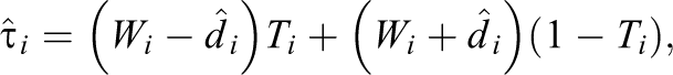
where
Recall that for Bernoulli randomized experiments, Equation (1) is an unbiased estimate of the average treatment effect if
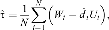
We define an estimate of the average treatment effect as

in which we estimate di
by using a leave-one-out procedure. We will refer to this sample splitting estimator as the paired leave-one-out potential outcomes (P-LOOP) estimator. For each pair i, we drop both observations and use the remaining
To see why this estimator is generally an improvement over the simple difference estimator, we consider the baseline approach where we set
3.2. Asymptotic Normality
In this section, we demonstrate that Equation (2) is asymptotically normally distributed under certain regularity conditions. Consider an infinite sequence of pairs
We first define some additional notation. Let
For some intuition as to why Equation (2) converges to a normal distribution, consider the following decomposition:
The

to converge to 0, in which case average of the “remainder terms”
In order for this intuition to hold, the data and the imputation method used must be sufficiently well-behaved. We next present general assumptions regarding their behavior. Note that we do not necessarily prove that these assumptions hold for any specific prediction algorithm.
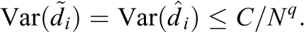
That is, as we observe more units, the variation of
In the case where

Moreover, the influence of pair j on


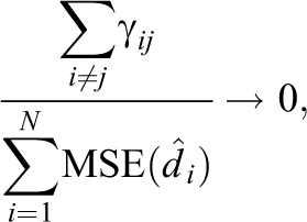
In other words, the expected value of the
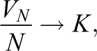
and

That is, the mean squared error of the imputation method converges to a value K. In addition, no single term of the mean squared error dominates the remaining terms.
When Assumptions 1 through 4 hold
3.3. Variance
We now estimate the variance of Equation (2). Let
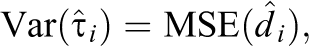
and thus that the variance is

where
under the conditions outlined in subsection 3.2. Because
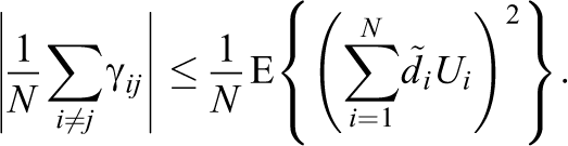
In online Appendix 4, we show that the mean squared error of
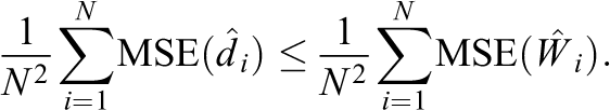
We can obtain an unbiased estimate for this upper bound, which we use to estimate the variance of
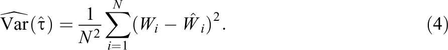
To compare this variance estimator to the variance estimator for the simple difference estimator, consider a special case where we estimate the average treatment effect without using covariates. In the absence of any covariate information, it would be logical to set
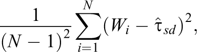
which is equal to
Importantly, because
4. Imputation Methods of Potential Differences in Paired Experiments
4.1. The Pair Inclusion Trade-Off
We next present an imputation method to address the pair inclusion trade-off discussed in Section 1. We first discuss this trade-off further and then propose a method for addressing the trade-off within the P-LOOP estimator. The pair inclusion trade-off is perhaps easiest to understand in the context of a linear model rather than the Neyman–Rubin model. Consider the following standard linear regression model

where Y is the observed outcome, T is the treatment assignment vector, Z is a covariate, and P is a
Several authors have compared the variance of the simple difference estimator for completely and pair randomized designs under the Neyman–Rubin model (e.g., see Imai, 2008; Pashley and Miratrix, 2017). The difference in variance under these designs can be either positive or negative. Similarly, it may be possible to reduce the variance of our estimate when making covariate adjustments by ignoring the pair assignments. However, Imai (2008) cautions against analyzing paired experiments as if they were completely randomized, noting that this can result in biased confidence intervals and hypothesis tests. Fortunately, this is not an issue with the P-LOOP estimator, as we always account for the paired design. We always drop both observations in each pair when estimating di
, and the decision to ignore or include the paired structure for the remaining observations only affects the adjustment term
When we discuss the inclusion or exclusion of the paired structure when imputing potential outcomes, we refer specifically to how we treat the remaining pairs when building a prediction model. If we ignore the paired structure when imputing potential outcomes, this means we fit a model to the remaining observations as individual units. If we include the paired structure when imputing potential outcomes, this means we fit a model to the remaining observations, treating each pair as a unit. Regardless of which approach we choose, the estimator remains design-based. For a given pair i, we always leave out both observations, and we wish to use the remaining observations such that we obtain the best estimate for di .
Suppose we ignore the paired structure of the data when we train our imputation model for the potential outcomes. In this case, we model the relationship between the covariates and the outcome overall rather than the relationship within pairs. However, if the relationship between the covariates and outcome within pairs is sufficiently different from the relationship overall, we could obtain a
Consider a hypothetical experiment in which a blood pressure medication is being tested on pairs of twins, and each pair belongs to either Ethnicity A or Ethnicity B. For each participant, we record a single covariate, an indicator for the presence of a genetic mutation. On average, participants with this mutation have blood pressure that is 5 units lower. Suppose this mutation is common in Ethnicity A and rare in Ethnicity B. However, for reasons unrelated to the mutation, Ethnicity A has a baseline blood pressure that is on average 10 units higher than the baseline for Ethnicity B. In this case, the presence of the mutation would be associated with higher blood pressure as Ethnicity A is more likely to have the mutation and also has a higher baseline blood pressure. However, within pairs, the presence of the mutation will be associated with lower blood pressure. If we ignore pair assignments when estimating di
, we would infer that the presence of the mutation is associated with a higher value of blood pressure. For a given pair, we would want the presence of the mutation to predict lower blood pressure. Thus, the prediction of the difference
It can be unclear whether we should account for the pair assignments when imputing the potential differences. To avoid data snooping, we propose an imputation method in the rest of this section that automatically addresses the trade-off. We first propose methods for calculating
4.2. Estimating di When Pairs Are Not Predictive: Impute Potential Outcomes Separately
We first estimate di
without accounting for the pair assignments for the observations outside of pair i. To do this, we drop both observations in pair i, then fit a model on the individual observations for the remaining pairs and separately impute all four potential outcomes (i.e.,
More specifically, for each pair i, we drop both observations in the pair. We then fit a prediction algorithm on the remaining observations, ignoring the pair assignments and treating each individual as a unit. For example, we could regress
4.3. Estimating di When Pairs Are Predictive: Impute Potential Differences Directly
Next, we propose a method that accounts for pair assignments when estimating di
. Rather than imputing the potential outcomes (
When treating the pairs as units, we have
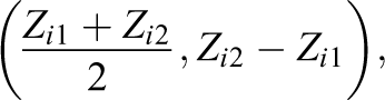
Alternatively, we may wish to transform the covariates in some way; for example, we could take the means and differences of the covariates. This is similar to the approaches used by Imbens and Rubin (2015) and Fogarty (2018). In this case, define Zi as

That is, Zi
is the vector where the first q entries are the averages of each covariate for the pair, and the second q entries are the differences (Observation 1 − Observation 2). In analogy to the concatenation example, we define
We can now estimate di
using these combined covariates and the observed differences. After leaving out pair i, we impute ai
by creating a model using the observed outcomes Wk
(for
into the model. Having obtained estimates
4.4. Interpolating Between Imputation Methods
We have proposed two methods for imputing potential outcomes. However, we often do not know ahead of time which method will perform better. We therefore adaptively interpolate between the two methods.
For each pair i, we have two estimates of ai
obtained using the two imputation methods described above. We refer to these estimates as
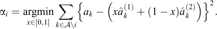
Taking the derivative with respect to x and setting equal to 0, we have

which we then restrict to be in the interval
5. Simulation Results
We present two simulations in the next two subsections. The first simulation illustrates the pair inclusion trade-off, while the second considers a scenario with a nonlinear relationship between the covariate and potential outcomes. In both cases, we compare the performance of P-LOOP with the simple difference estimator and the estimators discussed in Fogarty (2018), which we will refer to as Regression 1 and Regression 2. Regression 1 involves the treatment minus control outcomes regressed onto the treatment minus control covariates, while Regression 2 is the same regression with the addition of the mean of the covariates in each pair. For P-LOOP, recall from earlier that we are excluding the pair assignments in our imputation method if we impute the potential outcomes (
For each of the scenarios described below, we generate a single set of potential outcomes. Next, we generate 10,000 treatment assignment vectors. For each of these, we obtain a treatment effect estimate and the nominal variance (i.e., the estimated variance) using each estimator. This results in 10,000 point estimates and 10,000 variance estimates for each method, which we can use to estimate the true variance and the expectation of nominal variance for that method. We estimate the true variance as the variance of the 10,000 point estimates and the expectation of the nominal variance as the mean of the 10,000 nominal variances.
5.1. The Pair Inclusion Trade-Off
We consider a hypothetical experiment based off the scenario described in subsection 4.1, where we are interested in the effect of a blood pressure medication. We generate

where
Simulation 1 Results.

Note. True Var is the estimate for the true variance. E(Nom) refers to the estimate for the expected value of the nominal variance. For P-LOOP, these are estimates for expression of Equation (3) and for the expected value of Equation (4), respectively. Cov Pr is the estimated coverage proportion. We provide further details on how we obtain these estimates in online Appendix 6. The Monte Carlo estimates of the true variances have standard errors ranging from .002 to .007, while the Monte Carlo estimates for the expected values of the nominal variances all have standard errors below .0002. We provide these standard errors in online Appendix 6. P-LOOP = paired leave-one-out potential outcomes; RF = random forest; OLS = ordinary least squares.
We also generate a set of potential outcomes in which the pairs contain no additional information (beyond its association with covariate

where
We see that in the Simpson’s paradox case, imputing the potential outcomes separately (not accounting for pairs when estimating ai and bi ) causes inflated variance relative to the simple difference estimator, while imputing potential differences directly (accounting for pairs) results in improved performance. However, in the case where the pair assignments are uninformative, it is better to impute the potential outcomes separately. The gains in this example are relatively minor; however, we show in the later sections that the improvements can be more substantial.
5.2. A Nonlinear Scenario
In the previous example, the potential outcomes were generated from a linear model with independent, normally distributed noise. We examine a more complex scenario in this section. Consider a hypothetical experiment in which we are testing the effect of a drug on recovery time for an illness. We generate
The mean recovery time under treatment and control will be determined by the following logistic functions:
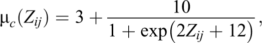
and
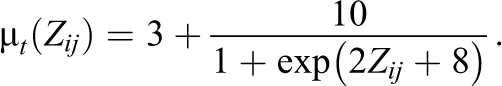
We then generate the control potential outcomes using γ random variables with shape parameter
Simulation 2 Results
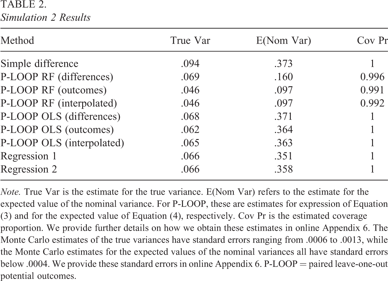
Note. True Var is the estimate for the true variance. E(Nom Var) refers to the estimate for the expected value of the nominal variance. For P-LOOP, these are estimates for expression of Equation (3) and for the expected value of Equation (4), respectively. Cov Pr is the estimated coverage proportion. We provide further details on how we obtain these estimates in online Appendix 6. The Monte Carlo estimates of the true variances have standard errors ranging from .0006 to .0013, while the Monte Carlo estimates for the expected values of the nominal variances all have standard errors below .0004. We provide these standard errors in online Appendix 6. P-LOOP = paired leave-one-out potential outcomes.
5.3. Remainder Terms
In this subsection, we investigate the quantity

for each of the data generating procedures used in the simulations discussed above. This quantity is of interest for several reasons. The convergence of Equation (5) to 0 plays an important role in proving the central limit theorem discussed in subsection 3.2. This convergence also implies that
It follows that the convergence of Equation (5) to 0 implies the convergence of
For each of the three data generating processes discussed in subsections 5.1 and 5.2, we generate potential outcomes and covariates for 1,000 pairs. We then consider each of the first
In Figure 1, we plot the estimated values of Equation (5) against the sample size N (both on a log base 10 scale). For each of the data generating procedures (and for both imputation methods), we can see that the estimated values of Equation (5) shrink to 0 as N increases. For the nonlinear data generating process, this decrease occurs more slowly when using random forest imputation. Note that Equation (5) contains terms relating to both the variances and covariances of the

We plot the estimated values of quantity of Equation (5) (i.e.,
6. Cognitive Tutor Impact Study
We apply our method to estimate the effect of an intervention in a randomized trial involving schools in Texas. This trial (discussed in Pane et al., 2014) tested the effectiveness of a computer program, the Cognitive Tutor Algebra 1 curriculum, and included 22 pairs of schools. The outcome of interest is the passing rate of the schools on the math section of the Texas Assessment of Knowledge and Skills in 2008. Available covariates included the school type (middle or high school) and a pretest score, the passing rate from 2007. We estimate the average treatment effect using either just the pretest score or both the pretest score and school type as covariates. In Table 3, we compare the performance of P-LOOP with the simple difference estimator and the estimators discussed in Fogarty (2018). We use random forests and linear regression as imputation methods in the P-LOOP estimator. As in the case of the simulations, we show the results imputing potential differences (accounting for pairs), imputing potential outcomes separately (ignoring the pair assignments), and the interpolation between the two. Note that P-LOOP imputing potential differences with OLS most closely matches the Regression 2 method, as both methods account for pairing and use the differences and averages of the covariates for making adjustments.
Comparison of Methods

Note. Point Est and Nominal Var refer to the point estimates and nominal variances for each method, respectively. P-LOOP = paired leave-one-out potential outcomes.
Both P-LOOP and the methods of Fogarty (2018) have smaller nominal variance than the unadjusted estimator. Regression 1 has lower variance than Regression 2 when the pretest score is the only covariate, but Regression 2 has lower variance when the school type is included. Both regression methods always account for the pair assignments. For the P-LOOP estimator, we see that it is better to impute the potential outcomes separately and that the interpolation method imputes values closer to the potential outcomes imputation. With the interpolation method, we do not lose out on the precision gains from ignoring the pairs in our imputation, but we are still protected against a potential Simpson’s paradox.
7. Discussion
In paired experiments, the design of the experiment helps to enforce covariate balance between the treatment and control groups. While this design is often effective, it can be useful to make covariate adjustments to further improve precision. Covariate adjustments in paired experiments share many of the issues in completely randomized experiments; for example, it can be unclear ahead of time which covariates to use. A unique issue to paired experiments is the pair inclusion trade-off, so we must take particular care when making adjustments in paired experiments. Failing to account for the pair assignments can harm performance (e.g., when a Simpson’s paradox occurs), while including the paired structure when the pair assignments are not predictive can needlessly inflate variance.
We present a design-based method for paired experiments, the P-LOOP estimator. This estimator is guaranteed to be unbiased by design. Nonetheless, the pair inclusion trade-off is still relevant because it affects the variance of the estimator. To the best of our knowledge, this method is the first to directly address the pair inclusion trade-off. Generally, other methods account for the pairing, which protects against Simpson’s paradox and other situations where the within-pair trends differ from the overall trend. However, our method imputes two sets of potential outcomes, one excluding and one including the pair assignments, and automatically interpolates between the two. As we see in the Texas Schools data, this allows for improved precision. The P-LOOP estimator is also the first method specifically for paired experiments that involves sample splitting and the use of machine learning methods to impute potential outcomes, building on the flexible approaches used in completely randomized experiments. This flexibility can be beneficial in several ways such as allowing for automatic variable selection or high-dimensional covariates. However, the leave-one-out approach can also be computationally intensive. If computation time is an issue, one can modify the procedure to leave out multiple pairs instead of single pairs at a time.
Finally, logical extensions to the P-LOOP estimator include block-randomized experiments and experiments with multiple treatments. As with paired experiments, it can be unclear whether to include the block assignments when making covariate adjustments. However, while paired experiments can be treated essentially as Bernoulli randomized experiments, this is not the case for blocked experiments, and the variance estimation procedure outlined in this article would necessarily be modified.
Supplemental Material
Supplemental Material, Appendix - Design-Based Covariate Adjustments in Paired Experiments
Supplemental Material, Appendix for Design-Based Covariate Adjustments in Paired Experiments by Edward Wu and Johann A. Gagnon-Bartsch in Journal of Educational and Behavioral Statistics
Footnotes
Acknowledgments
We would like to thank John Pane and Adam Sales for providing the data set used in Section 6.
Declaration of Conflicting Interests
The author(s) declared no potential conflicts of interest with respect to the research, authorship, and/or publication of this article.
Funding
The author(s) disclosed receipt of the following financial support for the research, authorship, and/or publication of this article: This article has been funded by Division of Mathematical Sciences (grant no: 1646108).
References
Supplementary Material
Please find the following supplemental material available below.
For Open Access articles published under a Creative Commons License, all supplemental material carries the same license as the article it is associated with.
For non-Open Access articles published, all supplemental material carries a non-exclusive license, and permission requests for re-use of supplemental material or any part of supplemental material shall be sent directly to the copyright owner as specified in the copyright notice associated with the article.