Design Considerations in Multisite Randomized Trials Probing Moderated Treatment Effects

Abstract

Past research has demonstrated that treatment effects frequently vary across sites (e.g., schools) and that such variation can be explained by site-level or individual-level variables (e.g., school size or gender). The purpose of this study is to develop a statistical framework and tools for the effective and efficient design of multisite randomized trials (MRTs) probing moderated treatment effects. The framework considers three core facets of such designs: (a) Level 1 and Level 2 moderators, (b) random and nonrandomly varying slopes (coefficients) of the treatment variable and its interaction terms with the moderators, and (c) binary and continuous moderators. We validate the formulas for calculating statistical power and the minimum detectable effect size difference with simulations, probe its sensitivity to model assumptions, execute the formulas in accessible software, demonstrate an application, and provide suggestions in designing MRTs probing moderated treatment effects.

Keywords

minimum detectable effect size difference moderated treatment effect multisite randomized trials (MRTs)statistical power

Recent efforts by a broad range of societies and funding agencies have emphasized rigorous study design as an important lever for improving the quality of evidence produced by impact evaluations (e.g., U.S. Department of Education & National Science Foundation, 2013). According to the Common Guidelines (2013), a joint report released by the National Science Foundation and the Institute of Education Sciences, designs which randomly assign units to conditions are the most rigorous designs and have the potential to yield the highest quality of evidence. Random assignment may occur at the individual level, as is the case of a multisite randomized trial (MRT) in which individuals (students) are randomly assigned to condition within sites (schools). Random assignment may also occur at the cluster level, as is the case of a cluster randomized trial (CRT), in which clusters (schools) are randomly assigned to condition and students are nested within schools. Although both MRTs and CRTs are common in impact studies in education (Spybrook & Raudenbush, 2009; Spybrook, Shi, & Kelcey, 2016), the focus of this article is the design of MRTs.

Initially, the focus of MRTs in education was to address “what works” questions or questions about main effects. More recently, researchers and policymakers have broadened the focus to include questions regarding “for whom, and under what circumstances” programs work, or questions about moderated treatment effects. The impetus for broadening the scope of questions stems in part from empirical research that suggests treatment effects frequently vary across site or individual characteristics (Weiss et al., 2017). Understanding the context in which an intervention is likely to be effective is fundamental to understanding the extent to which results are applicable and scalable to a wide range of schools and students and also facilitates the development of more nuanced theories.

In this study, we consider the design of MRTs that seek to answer questions about moderated treatment effects. Recall that in an MRT, individuals (students) are randomly assigned to condition within sites (schools). Hence, students represent Level 1 and schools represent Level 2 with treatment varying across Level 1 units. Our analyses consider the intersections of three facets of multilevel moderation that are common in practice: (a) Level 1 and Level 2 moderator variables, (b) random and nonrandomly varying slopes (coefficients) of the treatment variable and the interaction term between the treatment and moderator variables, and (c) binary and continuous moderators. We consider moderators at the student level (e.g., gender) and at the school level (e.g., school size, Title 1 status). For both levels, we consider binary and continuous moderators.

In planning an MRT, a key design consideration is the sample size necessary to achieve adequate statistical power (probability of detecting the main treatment effect and moderated treatment effect). A strong literature base exists for conducting power analyses for the main effects of MRTs already exist (e.g., Borenstein & Hedges, 2012; Dong & Maynard, 2013; Konstantopoulos, 2008; Raudenbush et al., 2011) and for conducting power analyses for main effects and moderator effects in CRTs (e.g., Dong et al., 2018; Spybrook, Kelcey, & Dong, 2016). However, there is less work on power calculations for moderated treatment effects in MRTs. Raudenbush and Liu (2000) developed power formulas for the site-level (Level 2) binary moderator effect in MRTs, and Bloom and Spybrook (2017) developed formulas for the minimum detectable effect size difference (MDESD) for the site-level binary moderator in MRTs. However, the scope of such studies has largely been limited to binary site-level moderators in MRTs. Missing from this literature is a more comprehensive statistical framework for power analyses of moderated treatment effects in MRTs that incorporates the considerations noted above (e.g., continuous moderators, random slopes) and a careful analysis delineating the parameters that govern power and their proportional influence (e.g., how does the intraclass correlation [ICC] coefficient or treatment effect variation/heterogeneity of coefficients affect power).

The purpose of this study is to develop a more comprehensive statistical framework and set of tools for the effective and efficient design of MRTs probing moderated treatment effects. As noted above, the framework we develop considers the intersections of three facets of multilevel moderation that are common in practice: (a) Level 1 and Level 2 moderator variables, (b) random and nonrandomly varying slopes (coefficients) of the treatment variable and the interaction term between the treatment and moderator variables, and (c) binary and continuous moderators. Our investigation of these facets developed formulas that delineate statistical power, the MDESD, and their corresponding confidence intervals (CIs). We also created software to assist researchers conducting power analyses for various moderated treatment effects.¹

This article is organized as follows: First, we outline a working example to provide the context to our formulations, structure, and expressions. Second, we present the formulas for the standard error (SE), statistical power, and the MDESD and its CIs for the moderator effect at Level 1 followed by Level 2. Within this scope, we first detail the case of continuous moderators with random slopes and then extend these cases to allow for binary moderators and nonrandomly varying slope models. We follow with Monte Carlo simulations to assess the validity of the formulas we derived. Third, we compare the statistical power and MDESD among the moderated treatment effect and main treatment effect both conceptually and practically followed by demonstrating the calculation of MDESD and power using several examples. We then summarize our findings and discuss the implications of powering for moderated treatment effects in the design of two-level MRTs. Finally, we conclude with considering directions for future work.

Working Example

We develop an illustrative example to frame our study. Our example focuses on a computer-assisted tutoring program intended to improve students’ reading achievement. For example, Chambers et al. (2008) used an MRT to test the effect of a computer-assisted tutoring program on reading achievement. The MRT included a total of 412 first graders randomly assigned to the computer-assisted tutoring or the traditional tutoring groups within each of 25 schools. The findings revealed no significant overall treatment effect. However, the study also suggested the potential for treatment effect heterogeneity. For instance, one common site- or school-level moderator variable that is commonly considered in moderation analyses is the average pretest. The follow-up question is how to design an MRT to systematically probe the moderated treatment effect of the computer-assisted tutoring program.

In this illustrative example and our larger study, we consider three design facets that are common in this literature. As outlined above, the first facet considers the level of the moderator (e.g., student vs. school level). For instance, the effect of the computer-assisted tutoring program may vary by the student characteristics (e.g., pretest and gender) or the site characteristics (e.g., average pretest). The levels of the moderators examine for whom (Level 1 moderators) and under what condition (Level 2 moderators) the computer-assisted tutoring program works.

The second facet concerns the quantitative nature of the moderator—that is, whether the moderator is binary (e.g., gender and program implementation [high vs. low]) or continuous (pretest and school size). When the moderator is a binary variable (e.g., gender), the moderator effect indicates the treatment effect difference between two categorical groups or the gender achievement gap in treatment effectiveness. When the moderator is a continuous variable (e.g., pretest), the moderator effect describes the disparate impact of the treatment on the outcome for different increments of the pretest.

The final facet examines whether the design calls for a random or nonrandomly varying term for the treatment and moderated treatment effects. More specifically, when the moderator is a Level 1 variable, the moderated treatment effect may randomly vary across sites (school) or be constant across schools. For instance, the treatment effect difference between males and females for the computer-assisted tutoring program may or may not be same across schools. In addition, at the school level, the treatment effect may still randomly vary across schools after accounting for the school-level moderator effect or may be constant across schools. For example, if the average pretest of a school explains some of the heterogeneity in treatment effects across schools but not all of it, there may be other factors contributing to the treatment effect heterogeneity. However, if the treatment effect is constant across schools after accounting for the differences among schools in terms of the average pretest, then it may be the only factor causing the treatment effect heterogeneity. The choice of random versus nonrandomly slope depends on the program theory and evidence from prior studies.

Statistical Power and the MDESD in Two-Level MRTs

Below we describe how we develop the formulas of the statistical power and the MDESD for Level 1 and Level 2 moderators in two-level MRTs. Suppose there are n students in each school, where a proportion (P) of the students within each school are randomly assigned to the treatment group to receive a computer-assisted tutoring intervention, and there are a total of J schools which serves as blocks or sites. The research questions include whether the effects of the tutoring intervention on student achievement vary by the students’ pretest or gender, or by the schools’ characteristics, and if the moderated treatment effects vary randomly across schools.

Random Slope Models

Random slope models allow us to test whether the treatment effect varies across moderator subgroups and whether the moderated treatment effects vary randomly across schools. To test for the Level 1 moderation, we use two-level random slope hierarchical linear modeling (HLM; Raudenbush & Bryk, 2002):

Level 1 : Y_{i j} = β_{0 j} + β_{1 j} T_{i j} + β_{2 j} T_{i j} M_{i j}^{(1)} + β_{3 j} M_{i j}^{(1)} + β_{4 j} X_{i j} + r_{i j}, r_{i j} \sim N (0, σ_{| T, M, X}^{2}) .

\begin{array}{l} Level 2 : β_{0 j} = γ_{00} + u_{0 j}, \\ β_{1 j} = γ_{10} + u_{1 j}, \\ β_{2 j} = γ_{20} + u_{2 j}, (\begin{matrix} u_{0 j} \\ u_{1 j} \\ u_{2 j} \end{matrix}) ~ N [(\begin{matrix} 0 \\ 0 \\ 0 \end{matrix}), (\begin{matrix} τ_{00}^{2} & τ_{01}^{} & τ_{02}^{} \\ τ_{11}^{2} & τ_{12}^{} \\ τ_{22}^{2} \end{matrix})] . \\ β_{3 j} = γ_{30}, \\ β_{4 j} = γ_{40} . \end{array}

The combined model is:

Y_{i j} = γ_{00} + (γ_{10} + u_{1 j}) T_{i j} + (γ_{20} + u_{2 j}) T_{i j} M_{i j}^{(1)} + γ_{30} M_{i j}^{(1)} + γ_{40} X_{i j} + u_{0 j} + r_{i j} .

$Y_{i j}$ is the achievement for student i in school j. The treatment variable, $T_{i j}$ , is a binary variable indicating whether the student receives the tutoring intervention (e.g., $T_{i j}$ = −0.5 for control, and 0.5 for treatment). $X_{i j}$ is a Level 1 covariate. $M_{i j}^{(1)}$ is a continuous Level 1 moderator, and $M_{i j}^{(1)} \sim N (0, S_{M^{(1)}}^{2})$ . $M_{i j}^{(1)}$ can be viewed as a grand-mean centered variable. The parameter, $γ_{10}$ , estimates the average treatment effect. $u_{1 j}$ represents the random site-specific deviation from the average treatment effect. Of interest for the moderator analysis is the collection of the site-specific moderation effects ( $β_{2 j}$ ) that can be summarized using the cross-site average moderated treatment effect ( $γ_{20}$ ) and the random site-specific deviation from that average ( $u_{2 j}$ ). We use $τ_{22}^{2}$ to describe the variance of u_2j and its covariances of $τ_{02}^{}$ and $τ_{12}^{}$ with the random effects for the intercept and treatment, respectively. Note that we use fixed slopes for the covariate ( $X_{i j}$ ) and moderator ( $M_{i j}^{(1)}$ ) because we focus on the setting in which random intercepts, treatment effects, and moderated treatment effects sufficiently capture variation among schools. In addition, it is often hard to estimate more than three random effects with sample sizes typical to these types of educational experiments. However, additional random slopes for covariates and the moderator are possible.

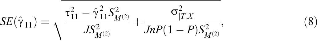
By extending Snijders’s (2001, 2005) work, the SE of the Level 1 moderator effect estimate ( ${\hat{γ}}_{20}$ ) in Model 3 can be expressed as (see Appendix A in the online version of the journal for details):

S E ({\hat{γ}}_{20}) = \sqrt{\frac{τ_{22}^{2}}{J} + \frac{σ_{| T, M, X}^{2}}{J n P (1 - P) S_{M^{(1)}}^{2}}} .

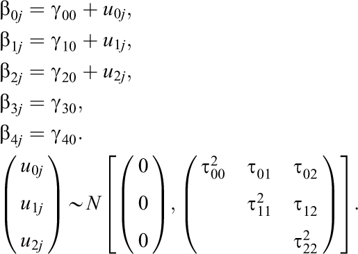
To test for the Level 2 moderation, we use two-level random slope HLM (Raudenbush & Bryk, 2002):

Level 1 : Y_{i j} = β_{0 j} + β_{1 j} T_{i j} + β_{2 j} X_{i j} + r_{i j}, r_{i j} \sim N (0, σ_{| T, X}^{2}) .

\begin{array}{l} Level 2 : β_{0 j} = γ_{00} + γ_{01} M_{j}^{(2)} + u_{0 j}, \\ β_{1 j} = γ_{10} + γ_{11} M_{j}^{(2)} + u_{1 j}, \\ β_{2 j} = γ_{20} . \end{array} (\begin{matrix} u_{0 j} \\ u_{1 j} \end{matrix}) \sim N [(\begin{matrix} 0 \\ 0 \end{matrix}), (\begin{matrix} τ_{00 | M}^{2} & τ_{01 | M}^{} \\ τ_{11 | M}^{2} \end{matrix})] .

The combined model is:

Y_{i j} = γ_{00} + γ_{01} M_{j}^{(2)} + (γ_{10} + γ_{11} M_{j}^{(2)} + u_{1 j}) T_{i j} + γ_{20} X_{i j} + u_{0 j} + r_{i j} .

$M_{j}^{(2)}$ is a continuous Level 2 moderator with distribution $M_{j}^{(2)} \sim N (0, S_{M^{(2)}}^{2})$ such that $M_{j}^{(2)}$ can again be seen as a grand-mean centered variable. $β_{1 j}$ estimates the site-specific treatment effects that include three components: (1) the average treatment effects across sites $(γ_{10})$ , (2) the average moderation effect ( $γ_{11}$ ) across sites, and (3) the random treatment effects across sites ( $u_{1 j}$ ). $u_{1 j}$ has a variance of ( $τ_{11 | M}^{2}$ ) and covariance of ( $τ_{10 | M}^{}$ ) with the intercept.

By extending Snijders’s (2001, 2005) work, the estimate of the SE of the Level 2 moderator effect estimate ( ${\hat{γ}}_{11}$ ) can be expressed as (see online Appendix A for details):

S E ({\hat{γ}}_{11}) = \sqrt{\frac{τ_{11}^{2} - {\hat{γ}}_{11}^{2} S_{M^{(2)}}^{2}}{J S_{M^{(2)}}^{2}} + \frac{σ_{| T, X}^{2}}{J n P (1 - P) S_{M^{(2)}}^{2}}},

where ${\hat{γ}}_{11}^{2} S_{M^{(2)}}^{2}$ represents the estimate of the variance in $τ_{11}^{2}$ explained by the moderator and $τ_{11}^{2}$ is the variance associated with the treatment effect in the model that is not conditional on Level 2 moderator (Model A4).

Power Formulas

We can test $γ_{20}$ and $γ_{11}$ using a t test. Assuming the alternative hypothesis is true, the test statistic follows a noncentral t distribution, T’, and the noncentrality parameters (unstandardized) for the moderator effects are as follows:

λ_{| M^{(1)}} = \frac{{\hat{γ}}_{20}}{\sqrt{\frac{τ_{22}^{2}}{J} + \frac{σ_{| T, M, X}^{2}}{J n P (1 - P) S_{M^{(1)}}^{2}}}}

and

λ_{| M^{(2)}} = \frac{{\hat{γ}}_{11}}{\sqrt{\frac{τ_{11}^{2} - {\hat{γ}}_{11}^{2} S_{M^{(2)}}^{2}}{J S_{M^{(2)}}^{2}} + \frac{σ_{| T, X}^{2}}{J n P (1 - P) S_{M^{(2)}}^{2}}}} .

We standardize the moderation effect variability across sites such that $ω_{t m}^{2} = τ_{22}^{2} / (τ_{00}^{2} + σ_{}^{2})$ with $σ_{}^{2}$ and $τ_{00}^{2}$ as the unconditional variances of residuals for Level 1 and Level 2 intercept (i.e., the model without any predictors). Similarly, we standardize the treatment effect variability across sites such that $ω_{t}^{2} = τ_{11}^{2} / (τ_{00}^{2} + σ_{}^{2})$ , which indicates the standardized treatment effect variability across sites in the model that is not conditional on Level 2 moderator, $M_{j}^{(2)}$ . $R_{1}^{2}$ is the proportion of variance at Level 1 that is explained by the Level 1 covariate, moderator, and treatment variable: $R_{1}^{2} = 1 - σ_{| T, M, X}^{2} / σ_{}^{2}$ ( $R_{1}^{2} = 1 - σ_{| T, X}^{2} / σ_{}^{2}$ for Level 2 moderation model). The standardized coefficients ${\hat{δ}}_{1 c} = {\hat{γ}}_{20} / \sqrt{τ_{00}^{2} + σ_{}^{2}}$ and ${\hat{δ}}_{2 c} = {\hat{γ}}_{11} / \sqrt{τ_{00}^{2} + σ_{}^{2}}$ , the unconditional ICC $ρ = τ_{00}^{2} / (τ_{00}^{2} + σ_{}^{2})$ , and $S_{M^{(1)}}^{2}$ = $S_{M^{(2)}}^{2}$ = 1, the standardized noncentrality parameters for Level 1 and Level 2 moderator effect are as follows:

λ_{| M^{(1)}} = \frac{{\hat{γ}}_{20}}{\sqrt{\frac{ω_{t m}^{2} (τ_{00}^{2} + σ_{}^{2})}{J} + \frac{(1 - R_{1}^{2}) σ_{}^{2}}{J n P (1 - P) S_{M^{(1)}}^{2}}}} = \frac{{\hat{δ}}_{1 c}}{\sqrt{\frac{ω_{t m}^{2}}{J} + \frac{(1 - R_{1}^{2}) (1 - ρ)}{J n P (1 - P)}}}

and

λ_{| M^{(2)}} = \frac{{\hat{γ}}_{11}}{\sqrt{\frac{(ω_{t}^{2} - {\hat{δ}}_{2 c}^{2} S_{M^{(2)}}^{2}) (τ_{00}^{2} + σ_{}^{2})}{J S_{M^{(2)}}^{2}} + \frac{(1 - R_{1}^{2}) σ_{}^{2}}{J n P (1 - P) S_{M^{(2)}}^{2}}}} = \frac{{\hat{δ}}_{2 c}}{\sqrt{\frac{ω_{t}^{2} - {\hat{δ}}_{2 c}^{2}}{J} + \frac{(1 - R_{1}^{2}) (1 - ρ)}{J n P (1 - P)}}} .

The degrees of freedom are v₁ = J − 1 and v₂ = J − 2, respectively.

The statistical power for a two-sided test is $1 - β = 1 - P [T^{'} (J - 1, λ_{| M^{(1)}}) < t_{0}] + P [T^{'} (J - 1, λ_{| M^{(1)}}) \leq - t_{0}]$ for a Level 1 moderator effect, where $t_{0} = t_{1 - \frac{α}{2}, J - 1'}$ and $1 - β = 1 - P [T^{'} (J - 2, λ_{| M^{(2)}}) < t_{0}] + P [T^{'} (J - 2, λ_{| M^{(2)}}) \leq - t_{0}]$ for a Level 2 moderator effect, where $t_{0} = t_{1 - \frac{α}{2}, J - 2'}$ .

When the Level 1 moderator, $M_{i j}^{(1)}$ , is a binary variable with a proportion of Q ₁ in one moderator subgroup and (1 − Q ₁) in another moderator subgroup, $M_{i j}^{(1)} \sim Bernoulli (Q_{1})$ :

VAR (M_{i j}^{(1)}) = S_{M^{(1)}}^{2} = Q_{1} (1 - Q_{1}) .

By inserting Equation 13 into Equation 9, we derived the standardized noncentrality parameters as

λ_{| M^{(1)}} = \frac{{\hat{δ}}_{1 b}}{\sqrt{\frac{ω_{t m}^{2}}{J} + \frac{(1 - R_{1}^{2}) (1 - ρ)}{J n P (1 - P) Q_{1} (1 - Q_{1})}}} .

Similarly, when the Level 2 moderator, $M_{j}^{(2)}$ , is a binary variable with a proportion of Q ₂ in one moderator subgroup and (1 − Q ₂) in another moderator subgroup, $M_{j}^{(2)} \sim Bernoulli (Q_{2})$ :

VAR (M_{j}^{(2)}) = S_{M^{(2)}}^{2} = Q_{2} (1 - Q_{2}) .

By inserting Equation 15 into Equation 10, we derived the standardized noncentrality parameters as

λ_{| M^{(2)}} = \frac{{\hat{δ}}_{2 b}}{\sqrt{\frac{ω_{t}^{2} - {\hat{δ}}_{2 b}^{2} Q_{2} (1 - Q_{2})}{J Q_{2} (1 - Q_{2})} + \frac{(1 - R_{1}^{2}) (1 - ρ)}{J n P (1 - P) Q_{2} (1 - Q_{2})}}} .

Note that Equation 16 above is consistent with Equation 26 in Raudenbush and Liu (2000) when P = Q ₂ = 0.5 and standardizing the within cluster variance as 1 ( $σ_{}^{2} = 1$ ).

The MDESD With CI

In addition to knowing the statistical power for a study to detect a desired effect size, it is useful to know the MDESD that a moderation study can detect with sufficient power (e.g., 80%) given sample sizes. The MDESD can be expressed as (Bloom, 1995, 2005, 2006; Dong et al., 2018; Murray, 1998)

MDESD (| \hat{δ} |) = M_{v} \times S E (\hat{γ}) / S D_{Y},

where $M_{v} = t_{α} + t_{1 - β}$ for one-tailed tests with v degrees of freedom, and $M_{v} = t_{α / 2} + t_{1 - β}$ for two-tailed tests. $S E (\hat{γ})$ is the SE of the moderation effect estimate as in Equations 4 and 8. $S D_{Y}$ is the standard deviation of the outcome measure (Y) and is defined as the square root of the total unconditional variance, $S D_{Y} = \sqrt{τ_{00}^{2} + σ_{}^{2}}$ .

Hence, by inserting Equation 4 into Equation 17, we derived the MDESD for the standardized coefficient for a continuous Level 1 moderator as

MDESD (| {\hat{δ}}_{1 c} |) = M_{v} \sqrt{\frac{τ_{22}^{2}}{J} + \frac{σ_{| T, M, X}^{2}}{J n P (1 - P) S_{M^{(1)}}^{2}}} / \sqrt{τ_{00}^{2} + σ_{}^{2}} = M_{v} \sqrt{\frac{ω_{t m}^{2}}{J} + \frac{(1 - R_{1}^{2}) (1 - ρ)}{J n P (1 - P)}},

where the standardized coefficient ( ${\hat{δ}}_{1 c}$ ), the standardized effect variability of the moderation across sites ( $ω_{t m}^{2}$ ), the proportion of variance at Level 1 ( $R_{1}^{2}$ ), the unconditional ICC ( $ρ$ ), and $S_{M^{(1)}}^{2}$ are defined as in Equation 12. The degrees of freedom is J − 1.

The 100 × (1−α)% CI for $MDESD (| {\hat{δ}}_{1 c} |)$ is given by

(M_{v} \pm t_{α / 2}) \sqrt{\frac{ω_{t m}^{2}}{J} + \frac{(1 - R_{1}^{2}) (1 - ρ)}{J n P (1 - P)}} .

The MDESD for the standardized mean difference for a binary Level 1 moderator is as follows:

MDESD (| {\hat{δ}}_{1 b} |) = M_{v} \sqrt{\frac{ω_{t m}^{2}}{J} + \frac{(1 - R_{1}^{2}) (1 - ρ)}{J n P (1 - P) Q_{1} (1 - Q_{1})}},

where the proportion (Q ₁) in one moderator subgroup is defined as in Equations 13 and 14, and the degrees of freedom is J − 1.

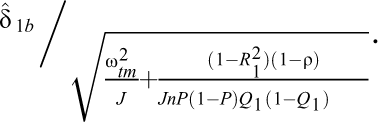
The 100 × (1−α)% CI for $MDESD (| {\hat{δ}}_{1 b} |)$ is given by

(M_{v} \pm t_{α / 2}) \sqrt{\frac{ω_{t m}^{2}}{J} + \frac{(1 - R_{1}^{2}) (1 - ρ)}{J n P (1 - P) Q_{1} (1 - Q_{1})}} .

By inserting Equation 8 into Equation 17, we derived the MDESD for the standardized coefficient for a continuous Level 2 moderator as

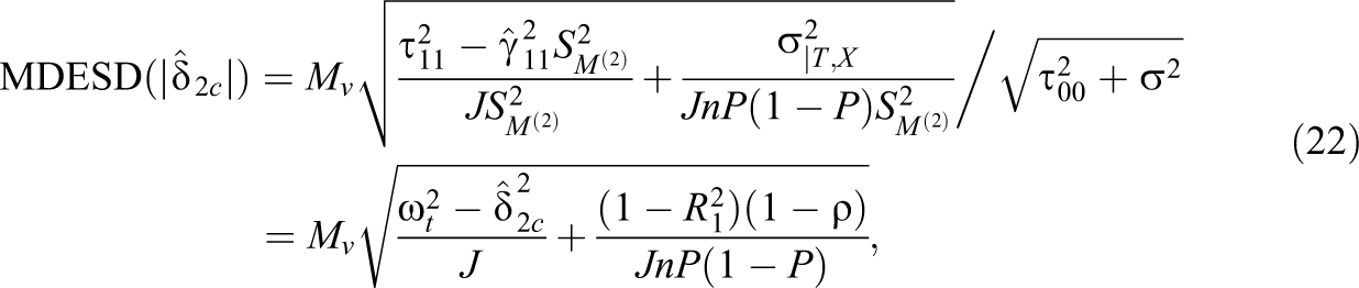
MDESD (| {\hat{δ}}_{2 c} |) = M_{v} \sqrt{\frac{τ_{11}^{2} - {\hat{γ}}_{11}^{2} S_{M^{(2)}}^{2}}{J S_{M^{(2)}}^{2}} + \frac{σ_{| T, X}^{2}}{J n P (1 - P) S_{M^{(2)}}^{2}}} / \sqrt{τ_{00}^{2} + σ_{}^{2}} = M_{v} \sqrt{\frac{ω_{t}^{2} - {\hat{δ}}_{2 c}^{2}}{J} + \frac{(1 - R_{1}^{2}) (1 - ρ)}{J n P (1 - P)}},

where the standardized coefficient ( ${\hat{δ}}_{2 c}$ ), the standardized treatment effect variability across sites ( $ω_{t}^{2}$ ), the proportion of variance at Level 1 ( $R_{1}^{2}$ ), the unconditional ICC ( $ρ$ ), and $S_{M^{(2)}}^{2}$ are defined as in Equation 12. Because ${\hat{δ}}_{2 c}$ is on both sides of Equation 22, we rearrange such that

MDESD (| {\hat{δ}}_{2 c} |) = M_{v} \sqrt{(\frac{ω_{t}^{2}}{J} + \frac{(1 - R_{1}^{2}) (1 - ρ)}{J n P (1 - P)}) / (1 + \frac{M_{v}^{2}}{J})},

where the degrees of freedom is J − 2.

The 100 × (1−α)% CI for $MDESD (| {\hat{δ}}_{2 c} |)$ is given by

(M_{v} \pm t_{α / 2}) \sqrt{(\frac{ω_{t}^{2}}{J} + \frac{(1 - R_{1}^{2}) (1 - ρ)}{J n P (1 - P)}) / (1 + \frac{M_{v}^{2}}{J})} .

The MDESD for the standardized mean difference for a binary Level 2 moderator is as follows:

MDESD (| {\hat{δ}}_{2 b} |) = M_{v} \sqrt{(\frac{ω_{t}^{2}}{J Q_{2} (1 - Q_{2})} + \frac{(1 - R_{1}^{2}) (1 - ρ)}{J n P (1 - P) Q_{2} (1 - Q_{2})}) / (1 + \frac{M_{v}^{2}}{J})},

where the degrees of freedom of J − 2.

The 100 × (1−α)% CI for $MDESD (| {\hat{δ}}_{2 b} |)$ is given by

(M_{v} \pm t_{α / 2}) \sqrt{(\frac{ω_{t}^{2}}{J Q_{2} (1 - Q_{2})} + \frac{(1 - R_{1}^{2}) (1 - ρ)}{J n P (1 - P) Q_{2} (1 - Q_{2})}) / (1 + \frac{M_{v}^{2}}{J})} .

Table 1 presents the summary of standardized noncentrality parameters, MDESD and 100 × (1−α)% CIs, and degrees of freedom for the t test for various moderated treatment effects in two-level MRTS. The above results are presented under Models “MRT2-1R-1” and “MRT2-1R-2,” which stands for a two-level MRT with a Level 1 and Level 2 moderators with random moderator effects.

Table 1.

Summary of Standardized Noncentrality Parameters, MDESD, and 100 × (1−α)% Confidence Intervals (CIs) for Two-Level MRTs

Model Number	HLM	Standardized Noncentrality Parameter (λ)	MDESD and 100 × (1−α)% CI	Degree of Freedom (v)
MRT2-1R-1	L1: $\begin{array}{l} Y_{i j} = β_{0 j} + β_{1 j} T_{i j} + β_{2 j} T_{i j} M_{i j}^{(1)} + β_{3 j} M_{i j}^{(1)} \\ + β_{4 j} X_{i j} + r_{i j}, r_{i j} \sim N (0, σ_{\| T, M, X}^{2}) . \end{array}$ L2: $\begin{array}{l} β_{0 j} = γ_{00} + γ_{01} M_{j}^{(2)} + u_{0 j}, \\ β_{1 j} = γ_{10} + γ_{11} M_{j}^{(2)} + u_{1 j}, (\begin{matrix} u_{0 j} \\ u_{1 j} \end{matrix}) ~ N [(\begin{matrix} 0 \\ 0 \end{matrix}), (\begin{matrix} τ_{00 \| M}^{2} & τ_{01 \| M}^{} \\ τ_{11 \| M}^{2} \end{matrix})] . \\ β_{2 j} = γ_{20} . \end{array}$	Binary moderator: $\frac{{\hat{δ}}_{1 b}}{\sqrt{\frac{ω_{t m}^{2}}{J} + \frac{(1 - R_{1}^{2}) (1 - ρ)}{J n P (1 - P) Q_{1} (1 - Q_{1})}}} .$ Continuous moderator: $\frac{{\hat{δ}}_{1 c}}{\sqrt{\frac{ω_{t m}^{2}}{J} + \frac{(1 - R_{1}^{2}) (1 - ρ)}{J n P (1 - P)}}} .$	Binary moderator: $M_{v} \sqrt{\frac{ω_{t m}^{2}}{J} + \frac{(1 - R_{1}^{2}) (1 - ρ)}{J n P (1 - P) Q_{1} (1 - Q_{1})}} .$ $(M_{v} \pm t_{α / 2}) \sqrt{\frac{ω_{t m}^{2}}{J} + \frac{(1 - R_{1}^{2}) (1 - ρ)}{J n P (1 - P) Q_{1} (1 - Q_{1})}} .$ Continuous moderator: $M_{v} \sqrt{\frac{ω_{t m}^{2}}{J} + \frac{(1 - R_{1}^{2}) (1 - ρ)}{J n P (1 - P)}} .$ $(M_{v} \pm t_{α / 2}) \sqrt{\frac{ω_{t m}^{2}}{J} + \frac{(1 - R_{1}^{2}) (1 - ρ)}{J n P (1 - P)}} .$	J − 1
MRT2-1R-2	L1: $Y_{i j} = β_{0 j} + β_{1 j} T_{i j} + β_{2 j} X_{i j} + r_{i j}, r_{i j} \sim N (0, σ_{\| T, M, X}^{2}) .$ L2: $\begin{array}{l} β_{0 j} = γ_{00} + γ_{01} M_{j}^{(2)} + u_{0 j}, \\ β_{1 j} = γ_{10} + γ_{11} M_{j}^{(2)} + u_{1 j}, (\begin{matrix} u_{0 j} \\ u_{1 j} \end{matrix}) ~ N [(\begin{matrix} 0 \\ 0 \end{matrix}), (\begin{matrix} τ_{00 \| M}^{2} & τ_{01 \| M}^{} \\ τ_{11 \| M}^{2} \end{matrix})] . \\ β_{2 j} = γ_{20} . \end{array}$	Binary moderator: $\frac{{\hat{δ}}_{2 b}}{\sqrt{\frac{ω_{t}^{2} - {\hat{δ}}_{2 c}^{2} Q_{2} (1 - Q_{2})}{J Q_{2} (1 - Q_{2})} + \frac{(1 - R_{1}^{2}) (1 - ρ)}{J n P (1 - P) Q_{2} (1 - Q_{2})}}} .$ Continuous moderator: $\frac{{\hat{δ}}_{2 c}}{\sqrt{\frac{ω_{t}^{2} - {\hat{δ}}_{2 c}^{2}}{J} + \frac{(1 - R_{1}^{2}) (1 - ρ)}{J n P (1 - P)}}} .$	Binary moderator: $M_{v} \sqrt{(\frac{ω_{t}^{2}}{J Q_{2} (1 - Q_{2})} + \frac{(1 - R_{1}^{2}) (1 - ρ)}{J n P (1 - P) Q_{2} (1 - Q_{2})}) / (1 + \frac{M_{v}^{2}}{J})} .$ $(M_{v} \pm t_{α / 2}) \sqrt{(\frac{ω_{t}^{2}}{J Q_{2} (1 - Q_{2})} + \frac{(1 - R_{1}^{2}) (1 - ρ)}{J n P (1 - P) Q_{2} (1 - Q_{2})}) / (1 + \frac{M_{v}^{2}}{J})} .$ Continuous moderator: $M_{v} \sqrt{(\frac{ω_{t}^{2}}{J} + \frac{(1 - R_{1}^{2}) (1 - ρ)}{J n P (1 - P)}) / (1 + \frac{M_{v}^{2}}{J})} .$ $(M_{v} \pm t_{α / 2}) \sqrt{(\frac{ω_{t}^{2}}{J} + \frac{(1 - R_{1}^{2}) (1 - ρ)}{J n P (1 - P)}) / (1 + \frac{M_{v}^{2}}{J})} .$	J − 2
MRT2-1N-1	L1: $Y_{i j} = β_{0 j} + β_{1 j} T_{i j} + β_{2 j} T_{i j} M_{i j}^{(1)} + β_{3 j} M_{i j}^{(1)} + β_{4 j} X_{i j} + r_{i j}, r_{i j} \sim N (0, σ_{\| T, M, X}^{2}) .$ L2: $\begin{array}{l} β_{0 j} = γ_{00} + u_{0 j}, \\ β_{1 j} = γ_{10}, \\ β_{2 j} = γ_{20}, u_{0 j} ~ N (0, τ_{00}^{2}) \\ β_{3 j} = γ_{30}, \\ β_{4 j} = γ_{40} . \end{array}$	Binary moderator: $\frac{{\hat{δ}}_{1 b}}{\sqrt{\frac{(1 - R_{1}^{2}) (1 - ρ)}{J n P (1 - P) Q_{1} (1 - Q_{1})}}} .$ Continuous moderator: $\frac{{\hat{δ}}_{1 c}}{\sqrt{\frac{(1 - R_{1}^{2}) (1 - ρ)}{J n P (1 - P)}}} .$	Binary moderator: $M_{v} \sqrt{\frac{(1 - R_{1}^{2}) (1 - ρ)}{J n P (1 - P) Q_{1} (1 - Q_{1})}} .$ $(M_{v} \pm t_{α / 2}) \sqrt{\frac{(1 - R_{1}^{2}) (1 - ρ)}{J n P (1 - P) Q_{1} (1 - Q_{1})}} .$ Continuous moderator: $M_{v} \sqrt{\frac{(1 - R_{1}^{2}) (1 - ρ)}{J n P (1 - P)}} .$ $(M_{v} \pm t_{α / 2}) \sqrt{\frac{(1 - R_{1}^{2}) (1 - ρ)}{J n P (1 - P)}} .$	J(n − 1) − 4
MRT2-1N-2	L1: $Y_{i j} = β_{0 j} + β_{1 j} T_{i j} + β_{2 j} X_{i j} + r_{i j}, r_{i j} \sim N (0, σ_{\| T, M, X}^{2}) .$ L2: $\begin{array}{l} β_{0 j} = γ_{00} + γ_{01} M_{j}^{(2)} + u_{0 j}, \\ β_{1 j} = γ_{10} + γ_{11} M_{j}^{(2)}, u_{0 j} ~ N (0, τ_{00}^{2}) . \\ β_{2 j} = γ_{20} . \end{array}$	Binary moderator: $\frac{{\hat{δ}}_{2 b}}{\sqrt{\frac{(1 - R_{1}^{2}) (1 - ρ)}{J n P (1 - P) Q_{2} (1 - Q_{2})}}} .$ Continuous moderator: $\frac{{\hat{δ}}_{2 c}}{\sqrt{\frac{(1 - R_{1}^{2}) (1 - ρ)}{J n P (1 - P)}}} .$	Binary moderator: $M_{v} \sqrt{\frac{(1 - R_{1}^{2}) (1 - ρ)}{J n P (1 - P) Q_{2} (1 - Q_{2})}} .$ $(M_{v} \pm t_{α / 2}) \sqrt{\frac{(1 - R_{1}^{2}) (1 - ρ)}{J n P (1 - P) Q_{2} (1 - Q_{2})}} .$ Continuous moderator: $M_{v} \sqrt{\frac{(1 - R_{1}^{2}) (1 - ρ)}{J n P (1 - P)}} .$ $(M_{v} \pm t_{α / 2}) \sqrt{\frac{(1 - R_{1}^{2}) (1 - ρ)}{J n P (1 - P)}} .$	J(n − 1) − 3

Note. MRT2-1R-1 and MRT2-1R-2 stand for two-level MRTs with a Level 1 and a Level 2 moderator with random slopes, respectively. MRT2-1N-1 and MRT2-1N-2 stand for two-level MRTs with a Level 1 and a Level 2 moderator with nonrandomly varying slopes, respectively. MDESD = minimum detectable effect size difference.

Nonrandomly Varying Slope Models

The hierarchical linear models with a nonrandomly varying slope assume that the treatment effect varies by the moderators but does not randomly vary across sites (Models MRT2-1N-1 and MRT2-1N-2 in Table 1 and below).

The models with a nonrandomly varying slope for a Level 1 moderator (MRT2-1N-1) are as follows:

L 1 : Y_{i j} = β_{0 j} + β_{1 j} T_{i j} + β_{2 j} T_{i j} M_{i j}^{(1)} + β_{3 j} M_{i j}^{(1)} + β_{4 j} X_{i j} + r_{i j}, r_{i j} \sim N (0, σ_{| T, M, X}^{2}) .

\begin{array}{l} L 2 : β_{0 j} = γ_{00} + u_{0 j}, u_{0 j} \sim N (0, τ_{00}^{2}), \\ β_{1 j} = γ_{10}, \\ β_{2 j} = γ_{20}, \\ β_{3 j} = γ_{30}, \\ β_{4 j} = γ_{40} . \end{array}

The models with a non-randomly varying slope for a Level 2 moderator (MRT2-1N-2) are as follows:

Level 1 : Y_{i j} = β_{0 j} + β_{1 j} T_{i j} + β_{2 j} X_{i j} + r_{i j}, r_{i j} \sim N (0, σ_{| T, X}^{2}) .

\begin{array}{l} Level 2 : β_{0 j} = γ_{00} + γ_{01} M_{j}^{(2)} + u_{0 j}, u_{0 j} \sim N (0, τ_{00}^{2}), \\ β_{1 j} = γ_{10} + γ_{11} M_{j}^{(2)}, \\ β_{2 j} = γ_{20} . \end{array}

The nonrandomly varying slope model is a special case of the random slope model. Setting $ω_{t x}$ = $ω_{t}$ = 0 in Equations 11, 12, 14, 16, and 18 –26, the formulas can be used for calculating statistical power and MDESD for nonrandomly varying slope models. The degrees of freedom are $J (n - 1) - 4$ for Level 1 and $J (n - 1) - 3$ for Level 2 moderator effects. The standardized noncentrality parameters, MDESD and 100 × (1−α)% CIs, and degrees of freedom for the t test for Models “MRT2-1R-1” and “MRT2-1R-2” are summarized in Table 1.

Monte Carlo Simulations

To validate the SE and power formulas we derived, we conducted a Monte Carlo simulation to examine whether the formulas were consistent with the simulated results. The procedures for the Monte Carlo simulation are below:

We generated data using the hierarchical linear models in Equations 1 and 2, and 5 and 6 for random slope models with Level 1 and Level 2 moderators, respectively, Equations 27 and 28, and 29 and 30 for nonrandomly varying slope models with Level 1 and Level 2 moderators, respectively.

We used SAS PROC MIXED to analyze the data sets. We computed the SEs using the Kacker and Harville (1984) approximation, and the degrees of freedom are calculated using the Kenward and Roger (1997) method, which is recommended for small sample size (Verbeke & Molenberghs, 2000, p. 57). We calculated the moderator effect, standardized effect variability of the Level 1 moderation across sites ( $ω_{t m}^{2}$ ), and proportions of variance ( $R_{1}^{2}$ ) explained by Level 1 covariates using the same estimation models as the models for generating data, estimate the standardized treatment effect variability across sites ( $ω_{t}^{2}$ ) using the estimation models that only included the treatment variable, and estimate the unconditional ICC using the unconditional hierarchical linear models.

The moderator effect was standardized to the standardized mean difference for the binary moderators or the standardized coefficient for the continuous moderators; a p value of the moderator effect that is less than .05 was coded a rejection of the null hypothesis of no moderation.

We replicated Steps 1 through 3 2,000 times and calculated the means of the moderator effect size, $ω_{t m}^{2}$ , $ω_{t}^{2}$ , R ², and unconditional ICC; The standard deviation of 2,000 moderator effect sizes served as the SE estimate based on the empirical distribution of the moderator effect; we also calculated the SE based on our formulas and constructed the 95% CI for each point estimate; we calculate the absolute difference and relative difference between the SEs based on our formulas and that from the empirical distribution; we calculate the coverage rate of the 95% CI as the percentage of the 95% CI based on our formulas covering the true moderator effect. The proportion of times the null was rejected across the 2,000 replications estimated the Type I error rate when the moderation effect was set to 0 and the empirical power when the moderation effect was not set as 0; we compared the power and Type I error rate calculated from our derived formulas with those estimated from simulation.

Our Monte Carlo simulation considered several scenarios by changing the sample size, the moderator effect size, random slopes and nonrandomly varying slopes, and binary and continuous Level 1 and Level 2 moderators.

Tables 2 through 5 present the results of SE and power (or Type I error rate) estimates from the Monte Carlo simulation and that were calculated based on the formulas using the same design parameters and the coverage rate of 95% CI. The results provided evidence of the close correspondence on SEs and power (or Type I error) between our formulas and the empirical distribution from the simulation. For example, in all scenarios, the absolute difference and relative difference between the SE based on the empirical distribution of the moderator effect estimates and SE calculated from our formulas range from −0.007 to 0.005 and from −7.23% to 3.51%, respectively. The coverage rate of the 95% CI ranges from 0.93 to 0.96. The differences between the power calculated from the formulas and that estimated from simulation ranges from −0.006 to 0.039.

Table 2.

Coverage of 95% Confidence Interval (CI) and Power (Type I Error Rate) From Monte Carlo Simulation and the Formulas for a Continuous Moderator With Random Slopes

	Level 1 Moderator				Level 2 Moderator
	Power		Type I Error		Power		Type I Error
Effect size difference	0.249	0.251	−0.001	0.000	0.253	0.253	0.003	−0.003
$ρ$	0.241	0.245	0.242	0.246	0.242	0.247	0.243	0.246
$ω_{t m}^{2}$ or $ω_{t}^{2}$	0.149	0.151	0.150	0.151	0.216	0.213	0.153	0.148
$R_{1}^{2}$	0.497	0.500	0.500	0.502	0.500	0.501	0.500	0.500
J (# of sites)	20	40	20	40	20	40	20	40
SE from simulation	0.110	0.078	0.109	0.077	0.113	0.078	0.114	0.081
SE from formula	0.106	0.075	0.106	0.075	0.107	0.075	0.107	0.075
Absolute difference in SE	−0.004	−0.003	−0.003	−0.002	−0.006	−0.004	−0.007	−0.006
Relative difference in SEs (%)	−3.382	−3.815	−2.606	−2.155	−5.508	−4.485	−6.199	−7.628
Coverage rate of 95% CI	0.960	0.944	0.961	0.957	0.950	0.946	0.953	0.936
Power/Type I error rate from simulation	0.572	0.887	0.044	0.042	0.575	0.888	0.048	0.060
Power/Type I error rate from formulas	0.592	0.903	0.050	0.050	0.611	0.909	0.050	0.050
Absolute difference	0.020	0.016	0.006	0.009	0.037	0.021	0.003	−0.009

Note. Results were based on 2,000 replications. $ω_{t m}^{2}$ is for Level 1 moderator; $ω_{t}^{2}$ is for Level 2 moderator. $R_{1}^{2}$ is the proportion of variance at Level 1 explained by Level 1 covariates. Sample size per site (n) is 20. The proportion of clusters assigned to the treatment group, P = 0.5. The 95% CI were constructed from the standard error that was calculated from formulas at $α$ = 0.05. Coverage rates were calculated based on percent of times that the 95% CIs included the true moderator effect.

Table 3.

Coverage of 95% Confidence Interval (CI) and Power (Type I Error Rate) From Monte Carlo Simulation and the Formulas for a Binary Moderator With Random Slopes

	Level 1 Moderator				Level 2 Moderator
	Power		Type I Error		Power		Type I Error
Effect size difference	0.248	0.251	−0.001	−0.001	0.249	0.252	−0.006	0.000
$ρ$	0.247	0.248	0.245	0.247	0.247	0.247	0.248	0.247
$ω_{t m}^{2}$ or $ω_{t}^{2}$	0.148	0.151	0.152	0.149	0.166	0.166	0.149	0.150
$R_{1}^{2}$	0.493	0.502	0.502	0.501	0.501	0.501	0.500	0.501
J (# of sites)	40	80	40	80	40	80	40	80
SE from simulation	0.114	0.076	0.111	0.077	0.149	0.106	0.151	0.106
SE from formula	0.106	0.075	0.106	0.075	0.150	0.106	0.150	0.106
Absolute difference in SE	−0.007	−0.001	−0.004	−0.002	0.002	0.000	−0.001	0.000
Relative difference in SEs (%)	−6.392	−1.392	−4.039	−2.366	1.166	0.031	−0.563	−0.235
Coverage rate of 95% CI	0.939	0.954	0.946	0.941	0.960	0.950	0.957	0.949
Power/Type I error rate from simulation	0.608	0.897	0.053	0.052	0.371	0.642	0.049	0.053
Power/Type I error rate from formulas	0.622	0.910	0.050	0.050	0.365	0.650	0.050	0.050
Absolute difference	0.014	0.013	−0.002	−0.001	−0.006	0.009	0.001	−0.002

Note. Results were based on 2,000 replications. $ω_{t m}^{2}$ is for Level 1 moderator; $ω_{t}^{2}$ is for Level 2 moderator. $R_{1}^{2}$ is the proportion of variance at Level 1 explained by Level 1 covariates. Sample size per site (n) is 20. The proportion of clusters assigned to the treatment group, P = 0.5. The proportion of the individuals/sites in one moderator subgroup, Q ₁ = Q ₂ = 0.5. The 95% CIs were constructed from the standard error that was calculated from formulas at $α$ = 0.05. Coverage rates were calculated based on percent of times that the 95% CIs included the true moderator effect.

Table 4.

Coverage of 95% Confidence Interval (CI) and Power (Type I Error Rate) From Monte Carlo Simulation and the Formulas for a Continuous Moderator With Nonrandomly Varying Slopes

	Level 1 Moderator				Level 2 Moderator
	Power		Type I Error		Power		Type I Error
Effect size difference	0.150	0.150	0.003	−0.002	0.152	0.150	0.002	0.000
$ρ$	0.245	0.246	0.245	0.248	0.245	0.247	0.246	0.245
$R_{1}^{2}$	0.498	0.500	0.498	0.498	0.499	0.499	0.498	0.499
J (# of sites)	20	40	20	40	20	40	20	40
SE from simulation	0.063	0.045	0.064	0.045	0.066	0.044	0.066	0.046
SE from formula	0.062	0.043	0.062	0.043	0.062	0.043	0.062	0.043
Absolute difference in SE	−0.001	−0.001	−0.002	−0.001	−0.005	−0.001	−0.004	−0.002
Relative difference in SEs (%)	−1.806	−2.507	−3.829	−2.513	−7.231	−1.373	−6.648	−4.659
Coverage rate of 95% CI	0.943	0.942	0.943	0.943	0.935	0.944	0.928	0.939
Power/Type I error rate from simulation	0.644	0.912	0.051	0.050	0.651	0.914	0.052	0.050
Power/Type I error rate from formulas	0.680	0.931	0.050	0.050	0.690	0.931	0.050	0.050
Absolute difference	0.036	0.019	0.000	0.001	0.039	0.017	−0.001	0.001

Note. Results were based on 2,000 replications. $R_{1}^{2}$ is the proportion of variance at Level 1 explained by Level 1 covariates. Sample size per site (n) is 20. The proportion of clusters assigned to the treatment group, P = 0.5. The 95% CIs were constructed from the standard error that was calculated from formulas at $α$ = 0.05. Coverage rates were calculated based on percent of times that the 95% CIs included the true moderator effect.

Table 5.

Coverage of 95% Confidence Interval (CI) and Power (Type I Error Rate) From Monte Carlo Simulation and the Formulas for a Binary Moderator With Nonrandomly Varying Slopes

	Level 1 Moderator				Level 2 Moderator
	Power		Type I Error		Power		Type I Error
Effect size difference	0.250	0.248	0.003	0.001	0.250	0.249	−0.004	0.003
$ρ$	0.246	0.250	0.243	0.248	0.249	0.251	0.251	0.249
$R_{1}^{2}$	0.490	0.490	0.498	0.499	0.498	0.500	0.498	0.500
J (# of sites)	20	40	20	40	20	40	20	40
SE from simulation	0.129	0.092	0.126	0.088	0.122	0.087	0.121	0.084
SE from formula	0.124	0.087	0.123	0.087	0.123	0.087	0.123	0.087
Absolute difference in SE	−0.005	−0.005	−0.002	−0.001	0.001	0.000	0.002	0.003
Relative difference in SEs (%)	−3.866	−5.036	−1.894	−1.634	0.863	−0.122	1.354	3.514
Coverage rate of 95% CI	0.955	0.942	0.958	0.959	0.953	0.957	0.961	0.950
Power/Type I error rate from simulation	0.520	0.791	0.049	0.043	0.525	0.811	0.041	0.052
Power/Type I error rate from formulas	0.520	0.809	0.050	0.050	0.528	0.819	0.050	0.050
Absolute difference	0.000	0.018	0.001	0.007	0.003	0.009	0.009	−0.001

Note. Results were based on 2,000 replications. $R_{1}^{2}$ is the proportion of variance at Level 1 explained by Level 1 covariates. Sample size per site (n) is 20. The proportion of clusters assigned to the treatment group, P = 0.5. The proportion of the individuals/sites in one moderator subgroup, Q ₁ = Q ₂ = 0.5. The 95% CIs were constructed from the standard error that was calculated from formulas at $α$ = 0.05. Coverage rates were calculated based on percent of times that the 95% CIs included the true moderator effect.

In addition, our derived formulas are based on the balanced design, that is, equal site sizes n_j = n, equal proportion of individuals assigned to the treatment group (P_j = P), and equal proportions of individuals in the moderator subgroup (Q_1j = Q₁ ) across sites. In practice, it is likely that the multisite moderation studies are imbalanced. For power analysis of the main effect in CRTs and MRTs, it is common to use the harmonic mean when the sample sizes across sites/clusters are imbalanced (Bloom, 2006; Konstantopoulos, 2010). We conducted a small simulation for MRTs with imbalanced n_j , P_j , and Q _1j using the similar procedures described above with some modifications. Specially, for MRTs with imbalanced sample sizes, sample size (n_j ) for site j ranges from 4 to 40, n_j increases 4 for every four sites when J = 40 and for every eight sites when J = 80. For MRTs with imbalanced P_j or Q _1j, P_j or Q _1j ranges from 0.3 to 0.7. P_j or Q _1j increases 0.1 for every eight sites with site number j when J = 40 and for every 16 sites when J = 80. We used our formulas to calculate power based on the arithmetic mean ( $\sum_{j = 1}^{J} n_{j} / J$ = 22), the harmonic mean ( $J / \sum_{j = 1}^{J} \frac{1}{n_{j}}$ = 14), and the geometric mean ( $\sqrt[J]{n_{1} \times \dots \times n_{j}}$ = 18), respectively. For imbalanced P_j or Q _1j, we calculated the arithmetic mean, the harmonic mean, and the geometric mean of their variance (P_j (1 − P_j ) or Q _1j(1 − Q_1j )), then solved for P or Q ₁. We also calculated power based on the balanced design. Table 6 presents the results of power from simulation and from the formulas for a binary moderator with random slopes with combinations of imbalanced n_j , P_j , and Q _1j.

Table 6.

Power From Monte Carlo Simulation and the Formulas for a Binary Moderator With Random Slopes With Imbalanced n_j , P_j , and Q _1j

	Level 1 Moderator		Level 2 Moderator
Effect size difference	0.250	0.251	0.249	0.247
$ρ$	0.267	0.269	0.258	0.259
$ω_{t m}^{2}$ or $ω_{t}^{2}$	0.151	0.151	0.165	0.164
$R_{1}^{2}$	0.490	0.490	0.496	0.496
J (# of sites)	40	80	40	80
Power from simulation	0.582	0.880	0.333	0.593
Power from formulas (arithmetic means: n = 22; P = 0.36; Q ₁ = 0.36)	0.613	0.898	0.370	0.638
Power from formulas (harmonic means: n = 14; P = 0.35; Q ₁ = 0.35)	0.472	0.775	0.319	0.562
Power from formulas (geometric means: n = 18; P = 0.36; Q ₁ = 0.36)	0.554	0.854	0.349	0.608
Power from formulas (balanced design: n = 22; P = 0.5; Q ₁ = 0.5)	0.660	0.927	0.378	0.650

Note. Results were based on 2,000 replications. $ω_{t m}^{2}$ is for Level 1 moderator; $ω_{t}^{2}$ is for Level 2 moderator. $R_{1}^{2}$ is the proportion of variance at Level 1 explained by Level 1 covariates. Sample size for site j (n_j ) ranges from 4 to 40. n_j increases 4 for every four sites when J = 40 and for every eight sites when J = 80. The proportion (P_j ) of individuals assigned to the treatment group in site j ranges from 0.3 to 0.7. P_j increases 0.1 for every eight sites with site number j when J = 40 and for every 16 sites when J = 80. The proportion (Q _1j) of individuals in the moderator subgroup 1 in site j ranges from 0.3 to 0.7. Q _1j increases 0.1 for every eight sites with site number j when J = 40 and for every 16 sites when J = 80. The proportion of the sites in the Level 2 moderator subgroup, Q ₂ = 0.5.

The results for the individual effects of imbalanced n_j , P_j , and Q _1j are presented in Tables B1 through B3 in online Appendix B. Our simulation suggests that the power calculation based on the harmonic mean underestimates the actual power and the power calculation based on the arithmetic mean overestimates the actual power. The power calculation based on the geometric mean approximates the power from the simulation very well. In addition, the imbalanced design has smaller power than balanced design as expected.

Furthermore, we derived our formulas when the continuous moderators are assumed to be normally distributed. In practice, the continuous moderators may not be normally distributed (Micceri, 1989). Although the conventional normality assumption for the linear models applies to the residuals, not the dependent variables or predictors, and linear models are robust to violations of the normality assumption when the sample size is large, we conducted a small Monte Carlo simulation to assess how the distributions of continuous moderators affect the estimated power. We used the SAS Macro RandFleishman (Wicklin, 2013), which implemented Fleishman’s (1978) cubic transformation method, to generate the variables with specified skewness and Pearson’s kurtosis. We simulated moderators with combined skewness (ranging from 1.18 to 1.95) and Pearson’s kurtosis (ranging from 2.21 to 7.44). The absolute difference between the power calculated from the formulas and that estimated from simulation ranged from 0.013 to 0.058. For many scenarios, the simulation results are very close to those from the power formulas. However, as the number of sites decreases the differences increase some, for example, the biggest difference (0.058) occurs for the smallest sample size of sites (J = 20; see Table B4 in online Appendix B). Overall, the results suggest that our formulas are fairly robust to violations of normality assumption for moderators; however, power can be overestimated when the sample size is small, and the normality assumption is violated.

We also simulated moderators with a bimodal distribution. The moderator variables were generated from the mixture distribution with two mixture components: one normal distribution (M = 1.4, variance = 0.3) with a mixture weight of 0.3, and another normal distribution (M = −0.6, variance = 0.1) with a mixture weight of 0.7. The results suggest that our formulas estimated the power fairly close to the simulation (absolute difference ranging from 0.013 to 0.039, Table B5 in online Appendix B).

Discussion: Comparisons Among Moderated Treatment Effects and Main Effect in MRTs

In this section, we compare the statistical power and MDESD among the moderation designs and main effect designs in two-level MRTs both conceptually (e.g., examining the formulas) and practically (e.g., using examples).

Contrasting Moderated Treatment Effects

Just as in the main effect analysis, the power of the moderated treatment effect in two-level MRTs is associated with the noncentrality parameter (λ) and the critical t value (t ₀). The critical t value (t ₀) is associated with the degrees of freedom (v), the Type I error rate ( $α$ ), and the choice of a one-tailed or two-tailed test. The noncentrality parameter (λ) is a ratio of the moderator effect estimate to its SE.

When the treatment effect varies by the moderator but does not vary across sites (i.e., nonrandomly varying effect; MRT2-1N-1 and MRT2-1N-2 in Table 1), the SE of the moderator effect is a function of the expected value of the aggregated Level 1 residual variance. The design parameters such as sample sizes for sites (J ) and individuals (n), the proportion of individuals in the treatment group (P), the proportion of variance at Level 1 explained by covariates ( $R_{1}^{2}$ ), and the unconditional ICC are associated with the SE and hence are associated with the power as the standardized noncentrality parameters suggest.

In particular, power increases with the sample sizes, and the sample sizes for sites (J ) and individuals (n) have the same effect on power and MDESD because it is the total sample size (Jn) that matters in the formulas for the standardized noncentrality parameters and MDESD for the nonrandomly varying effect models MRT2-1N-1 and MRT2-1N-2 (Table 1). Power increases when $R_{1}^{2}$ increases. Power also increases when the ICC increases because the larger ICC means that more variance is accounted for at the site level and less variance remains at the individual level, and our formulas indicate that the power of moderator effects in MRTs is associated with the Level 1 variance and not with the variance of the Level 2 intercept. Note that MRTs are different from CRTs in this regard. The power increases when P is close to 0.5, for example, a balanced design (P = 0.5) has the biggest power. In addition, the SE, MDESD, and noncentrality parameter formulas are the same for the Level 1 and Level 2 moderators. This suggests that the level of a moderator does not affect statistical power using the nonrandomly varying effect model.

If the moderator is a binary variable, the power is also associated with the proportion (Q) of the sample in one moderator subgroup. Compared with the results for the continuous moderators that use the standardized regression coefficient as the effect size metric, the results for the binary moderator that use the standardized mean difference as the effect size metric contain an additional factor of Q(1 − Q) that indicates the variance of the binary moderator. As a result, the MDESD using the standardized mean difference for the binary moderators is $\sqrt{\frac{1}{Q (1 - Q)}}$ times as large as the MDESD using the standardized regression coefficient for the continuous moderators.

If the treatment effect not only varies by the moderator but also varies across sites (i.e., random slope model; MRT2-1R-1 and MRT2-1R-2 in Table 1), the variance of the moderator effect estimate is a function of the variance of the parameter (i.e., true moderator effect) and the variance of the random error (Raudenbush & Bryk, 2002, pp. 44–45). As a result, the power is also associated with the effect heterogeneity across sites ( $ω_{t m}^{2}$ for the Level 1 moderator; $ω_{t}^{2}$ for the Level 2 moderator) in addition to the aggregated Level 1 residual variance. The MDESD increases and power decreases as $ω$ increases. The power (MDESD) of the random slope model is smaller (larger) than the nonrandomly varying slope model. The differences for the power and MDESD between the two models (random slope and nonrandomly varying slope models) decreases when the number of clusters (J) increases and the effect heterogeneity ( $ω$ ) decreases.

Comparing Moderated Treatment Effects With Main Effect

Based on the expression on page 48 in Dong and Maynard (2013), the minimum detectable effect size (MDES) for the main effect in a two-level MRT can be re-expressed as follows:

MDES = M_{v} \sqrt{(\frac{ω_{t}^{2}}{J} + \frac{(1 - R_{1}^{2}) (1 - ρ)}{J n P (1 - P)}) / (1 + \frac{M_{v}^{2}}{J})},

where the degrees of freedom (v) is J − 2, and all the design parameters are defined same as in Equation 25. Note that the MDES for the main effect uses the standardized mean difference as the effect size metric. We can compare the MDES with the MDESD for a binary moderator on the same effect size metric.

The ratio of the MDESD for a Level 2 binary random moderator effect to the MDES of the main effect is as follows:

\frac{MDESD (| {\hat{δ}}_{2 b} |)}{MDES} = \sqrt{\frac{1}{Q_{2} (1 - Q_{2})}} .

Equation 32 reveals that the MDESD is $\sqrt{\frac{1}{Q_{2} (1 - Q_{2})}}$ times large as the MDES in the same study design, which is twice when Q ₂ = 0.5.

Demonstration

In this section, we compare the MDESD/MDES and power among four moderated treatment effects and the main effect in a two-level MRT using several examples. The MDESD and power for the moderated treatment effects are calculated using the software we developed, which is a Microsoft Excel–based software package implementing formulas in Table 1. The MDES and power for the main effects are calculated using PowerUp! (Dong & Maynard, 2013). Suppose a team of researchers are designing a two-level MRT to test the efficacy of the computer-assisted tutoring intervention on mathematics achievement for the eighth graders. They are interested in student-level moderator effects and school-level moderator effects. They approach the moderator power analyses from two perspectives: (1) What is the MDESD given power of 0.80 and (2) what is the power for a meaningful moderation effect size.

Just like conducting a power analysis for the main effect, the researchers need to determine the meaningful effect size difference with practical significance they would like to detect and make reasonable assumptions of other design parameter values in their power analysis of moderator effects in MRTs. To determine the meaningful effect size differences, researchers may refer to the empirical benchmarks regarding normative expectations of annual gain, policy-relevant performance gaps, and moderation effect size results from similar studies (Bloom et al., 2008; Dong et al., 2016; Hill et al., 2008). For example, Hill et al. (2008) reported students’ math achievement gaps in effect size units from the National Assessment of Educational Progress in Grade 8 are −1.04 for Blacks versus Whites, −0.82 for Hispanics versus Whites, and −0.80 for the eligible versus ineligible for free/reduced-price lunch. The researchers may consider an effect size difference of 0.20 for the computer-assisted tutoring intervention to have a meaningful moderation effect because it is equivalent to one fifth a reduction of Black–White achievement gap and one fourth a reduction of Hispanic–White and eligible–ineligible for free/reduced-price lunch gaps. They may refer to moderation effect size results from similar studies; however, these results are very limited. For demonstration purposes, suppose they decide to use 0.20 as their desired effect size difference in their power analysis.

For other design parameter values, the researchers need to justify their choice based on the literature or pilot studies. Recently, several studies have reported the ICC and the proportion of variance explained by the covariates for academic achievement outcome measures (e.g., Bloom et al., 2007, and Hedges & Hedberg, 2007, 2013, on mathematics and reading; Westine et al., 2013, and Spybrook, Westine, & Taylor, 2016, on science achievement), outcome measures for teacher professional development (Kelcey & Phelps, 2013), and social and behavioral outcomes (Dong et al., 2016). The researchers assume a $ρ$ of 0.25, and the proportion of variance explained by the covariates at Level 1 of 0.5 ( $R_{1}^{2}$ = 0.5; Bloom et al., 2007; Hedges & Hedberg, 2007, 2013).

There are very few studies reporting the effect heterogeneity across sites values. We only identified Weiss et al. (2017) reporting the treatment effect heterogeneity values ( $ω_{t}^{2}$ ) across sites and did not identify any study reporting the heterogeneity values ( $ω_{t x}^{2}$ ) for the Level 1 moderated treatment effect across sites. Weiss et al. (2017) studied 51 outcome measures in 16 MRTs and reported that $ω_{t}^{2}$ ranged from 0 to 0.35, with 37% ranging from 0 to 0.05, 33% ranging from 0.05 to 0.15, and 29% ranging from 0.15 to 0.35. In this example, suppose the researchers decide to use the moderate effect size heterogeneity by assuming $ω_{t}^{2}$ = 0.05 and 0.15, respectively. Because there are no empirical reference values available for $ω_{t m}^{2}$ , they assume the same values of $ω_{t m}^{2}$ as $ω_{t}^{2}$ , that is, $ω_{t m}^{2}$ = $ω_{t}^{2}$ = 0.05 and 0.15, respectively. Note that the researchers may choose $ω_{t m}^{2}$ (and other design parameters) based on pilot studies, and we provide the SAS code to estimate these design parameters in online Appendix D (the SAS code and example data set can be downloaded from the website: https://www.causalevaluation.org/).

They use a balanced design with equal assignment of students to the treatment and control groups (P = 0.5) within a school (site) and 20 students per school. They are interested in the results for a binary moderator and a continuous moderator. For the binary case, they assume half of the sample is in one moderator subgroup (Q = 0.5). Table 7 shows the results of MDESD and power for the total numbers (J) of schools of 30 and 60 under the above assumptions. Tables C1 through C4 in online Appendix C provide examples of calculation of MDESD and power using our software.

Table 7.

MDESD and Statistical Power of Two-Level MRTs

Level of Moderator	Slope of Moderator Effect	MDESD				Power
		Binary Moderator		Continuous Moderator		Binary Moderator		Continuous Moderator
		J = 30	J = 60	J = 30	J = 60	J = 30	J = 60	J = 30	J = 60
1	Nonrandomly varying	.281	.198	.140	.099	.515	.807	.979	1.000
1	Random ( $ω_{t m}^{2}$ = 0.05)	.313	.218	.187	.130	.433	.731	.850	0.991
1	Random ( $ω_{t m}^{2}$ = 0.15)	.355	.247	.251	.174	.352	.622	.607	0.895
2	Nonrandomly varying	.281	.198	.140	.099	.515	.807	.979	1.000
2	Random ( $ω_{t}^{2}$ = 0.05)	.331	.244	.166	.122	.345	.613	.952	0.999
2	Random ( $ω_{t}^{2}$ = 0.15)	.444	.328	.222	.164	.207	.376	.691	0.943

Note. Under the assumptions: n = 20, $ρ$ = 0.25, P = 0.5, $R_{1}^{2}$ = 0.5, Q ₁ = Q ₂ = 0.5 for binary moderators, power = 0.8 for the calculation of MDESD, and effect size difference = 0.2 for the calculation of power, a two-sided test with α = 0.05. MDESD = minimum detectable effect size difference.

Furthermore, we demonstrate the relationship between power and total sample size of sites by comparing the main treatment effect design with four moderation designs with binary moderators in Figure 1A and 1B. The power was calculated independently for main effects and moderated effects based on the same assumptions as in Table 7: n = 20, $ρ$ = 0.25, P = 0.5, $R_{1}^{2}$ = 0.5, and Q ₁ = Q ₂ = 0.5. For the treatment effect heterogeneity, we set $ω_{t}^{2}$ = $ω_{t m}^{2}$ = 0.05 for the random slope design in Figure 1A and $ω_{t}^{2}$ = $ω_{t m}^{2}$ = 0.15 for the random slope design in Figure 1B. In addition, for comparison purposes, we assume the effect size (the standardized mean difference) for the main treatment effect and the effect size difference for the moderator effect at 0.2 using a two-sided test with α = 0.05. This is equivalent to effect sizes for the two moderator subgroups of 0.3 and 0.1, respectively. Thus, the resulting power curves are for the moderation analyses with a binary Level 2 moderator random effect (gray solid line), a binary Level 1 moderator random effect (long dotted line), a binary (Level 1 or Level 2) moderator with nonrandomly varying effect (short dotted line), and the main treatment effect (black solid line).

Figure 1.

Power versus site sample size. Note. Under the assumptions: n = 20, $R_{1}^{2}$ = 0.5, P = 0.5, Q ₁ = Q ₂ = 0.5, effect size (standardized mean difference) = 0.2, effect size difference = 0.2, and a two-sided test with α = 0.05. $ω_{t m}^{2}$ = $ω_{t}^{2}$ = 0.05 for random slope design in Figure 1A and $ω_{t m}^{2}$ = $ω_{t}^{2}$ = 0.15 for random slope design in Figure 1B.

The findings in Table 7, Figure 1A and 1B, and conceptual comparisons are discussed below. First, as for all power analyses, the power increases with the sample sizes (J and n). However, the importance of Level 1 and Level 2 sample sizes is different in different designs. Recall that the power and MDESD are same for Level 1 and Level 2 moderators with nonrandomly varying effects. This suggests that the sample sizes at Level 1 and Level 2 are equally important to the power and the MDESD for the nonrandomly varying moderator effect. In contrast, the sample size at Level 2 (J) is more important than Level 1 (n) for the moderator effect with the random slopes. Note that we set the site size (n) as 20 and vary the total number of sites (J) for demonstration in Table 7 and Figure 1A and 1B. In practice, researchers may choose n and J based on their research goals, budget, and sample availability. For example, the average n ranges from 11 to 1,176 and J ranges from 9 to 318 in 16 MRTs reported in Weiss et al. (2017). When it is not feasible for researchers to increase J, they may aim to increase n to increase statistical power.

Second, the proportion of the sample allocation to the treatment and control group (P) and to the moderator subgroup (Q) are related to the power and MDESD. The power (MDESD) increases (decreases) when P and Q is close to 0.5.

Third, the power (MDESD) increases (decreases) when the ICC increases. This is because the sites explain more Level 2 variance, reduce Level 1 variance, and hence reduce the SE of the moderated treatment effect estimates when $ρ$ increases.

Fourth, the power increases with the proportion of variance explained by the covariates ( $R_{1}^{2}$ ). A covariate can improve power through reducing the SE of the moderator effect estimate. Hence, in a two-level MRT, a Level 1 covariate ( $R_{1}^{2}$ > 0) can always improve power; however, a Level 2 moderator that is included in the intercept model at Level 2 does not contribute to the power.

Fifth, a design for detecting main effects always has larger power than detecting moderation effects in a two-level MRT. This is different from CRTs, in which, the power for detecting the effects of a Level 1 moderator with nonrandomly varying slope can be larger than the power for the main treatment effect analysis (Dong et al., 2018).

Sixth, the MDESD is larger or the power is smaller for a random moderator effect than a nonrandomly varying moderator effect. The differences for the power and MDESD between the two models (random slope and nonrandomly varying slope models) decreases when the number of clusters (J) increases and the effect heterogeneity ( $ω$ ) decreases. Note that we set the (moderated) treatment effect heterogeneity values, $ω_{t m}^{2}$ = $ω_{t}^{2}$ = 0.05 and 0.15, for the random slope designs based on the range of the moderate effect size heterogeneity reported by Weiss et al. (2017) for demonstration in Table 7 and Figure 1A and 1B. The power would be bigger/smaller if $ω_{t m}^{2}$ or $ω_{t}^{2}$ is smaller/bigger. In practice, researchers need to carefully justify the (moderated) treatment effect heterogeneity values. Finally, the MDESD as defined by the standardized mean difference for the binary moderator when Q = 0.5 is always twice the value of the MDESD defined by the standardized coefficient for the continuous moderator with a nonrandomly varying effect.

Conclusion

As researchers and policy makers are increasingly interested in the moderated treatment effects to answer the “what works for whom, and under what circumstances” questions in MRTs, a power analysis is a critical step. This study fills the gap in the literature by developing a more comprehensive statistical framework and software for power analyses to detect a wide variety of moderated treatment effects in MRTs. We provide some suggestions below.

First, we need to consider three facets of multilevel moderation that are common in practice: (a) Level 1 and Level 2 moderator variables, (b) random and nonrandomly varying slopes (coefficients) of the treatment variable and the interaction term between the treatment and moderator variables, and (c) binary and continuous moderators. We consider binary moderators (e.g., gender) when we are interested in detecting the treatment effect difference between boys and girls or whether the intervention can reduce boys–girls achievement gap; we consider continuous moderators (e.g., pretest) when we are interested in testing whether the association of pretest and posttest is different between the treatment and control groups or whether the treatment effect varies by the pretest. Sometimes we may dichotomize our continuous moderators to produce meaningful subgroups and facilitate the interpretation of moderated treatment effects. We consider Level 1 moderators (e.g., student characteristics) when we are interested in answering “for whom the program works,” and Level 2 moderators (e.g., school characteristics) when we are interested in answering “under what condition the program works.” Furthermore, we consider random (moderated) treatment effects when the theory or prior studies suggest that the (moderated) treatment effect may vary across sites and nonrandomly varying treatment effects otherwise. However, it would be beneficial to assume random effect if there is not clear theory or prior studies suggesting nonrandomly varying treatment effects.

Second, the power for all moderated treatment effects is smaller than the main effect in two-level MRTs. We need larger sample sizes to detect a moderated treatment effect with the same magnitude as the main effect. Regarding improving power, the sample size at the site level is more important than that at the individual level for random (moderated) treatment effects, and they are equally important for nonrandomly varying (moderated) treatment effects. Including Level 1 covariates that are correlated with the outcome, for example, pretest, can improve power. In addition, the power is bigger when the sample size is more balanced among the treatment-by-moderator groups and across sites, for example, the power is the maximum when P = 0.5 and Q ₁ or Q ₂ = 0.5 with equal site size. When the site size (n_j ), the proportion (P_j ) of individuals assigned to treatment group, or the proportion of individuals (Q _1j) in one moderator subgroup is imbalanced across sites (j), the power based on the harmonic mean is very conservative whereas the power based on the geometric mean approximates the power from the simulations very well and hence is what we recommend for power calculations.

This study focused on two-level MRTs. There are many important directions for further work. First, extending the work to three-level MRTs is necessary. For example, in three-level MRTs, where the treatment variable could be at Level 1 or Level 2, the moderator could be at any of three levels, and the (moderated) treatment effect can be either random or nonrandomly varying. The three-level MRTs provide more opportunities to probe moderated treatment effects. Second, accurate empirical estimates of the design parameters are critical for a power analysis. Hence, more empirical studies of design parameters (e.g., ICC, treatment effect heterogeneity, and meaningful size regarding the moderator effects) are important as we move forward.

Supplemental Material

Supplemental Material, 3.Appendix_2020.8.14 - Design Considerations in Multisite Randomized Trials Probing Moderated Treatment Effects

Supplemental Material, 3.Appendix_2020.8.14 for Design Considerations in Multisite Randomized Trials Probing Moderated Treatment Effects by Nianbo Dong, Benjamin Kelcey and Jessaca Spybrook in Journal of Educational and Behavioral Statistics

Footnotes

Declaration of Conflicting Interests

The author(s) declared no potential conflicts of interest with respect to the research, authorship, and/or publication of this article.

Funding

The author(s) disclosed receipt of the following financial support for the research, authorship, and/or publication of this article: This project has been funded by the National Science Foundation (1913563, 1552535, and 1760884). The opinions expressed herein are those of the authors and not the funding agency.

ORCID iD

Nianbo Dong

Note

References

Bloom

H. S.

(1995). Minimum detectable effects: A simple way to report the statistical power of experimental designs. Evaluation Review, 19(5), 547–556.

Bloom

H. S.

(2005). Randomizing groups to evaluate place-based programs. In Bloom

H. S.

(Ed.), Learning more from social experiments: Evolving analytic approaches (pp. 115–172). Russell Sage Foundation.

Bloom

H. S.

(2006). The core analytics of randomized experiments for social research (MDRC Working Papers on Research Methodology). http://www.mdrc.org/publications/437/full.pdf

Bloom

H. S.

Hill

C. J.

Black

A. B.

Lipsey

M. W.

(2008). Performance trajectories and performance gaps as achievement effect-size benchmarks for educational interventions. Journal of Research on Educational Effectiveness, 1(4), 289–328. http://doi.org/10.1080/19345740802400072

Bloom

H. S.

Richburg-Hayes

Black

A. R.

(2007). Using covariates to improve precision for studies that randomize schools to evaluate educational interventions. Educational Evaluation and Policy Analysis, 29(1), 30–59.

Bloom

H. S.

Spybrook

(2017). Assessing the precision of multisite trials for estimating the parameters of a cross-site population distribution of program effects. Journal of Research on Educational Effectiveness, 10(4), 877–902. http://doi.org/10.1080/19345747.2016.1271069

Borenstein

Hedges

L. V.

(2012). CRT-Power—Power analysis for cluster-randomized and multi-site studies [Computer software]. Biostat.

Chambers

Abrami

Tucker

Slavin

R. E.

Madden

N. A.

Cheung

Gifford

(2008). Computer-assisted tutoring in success for all: Reading outcomes for first graders. Journal of Research on Educational Effectiveness, 1(2), 120–137. http://doi.org/10.1080/19345740801941357

Dong

Kelcey

Spybrook

(2018). Power analyses of moderator effects in three-level cluster randomized trials. Journal of Experimental Education, 86(3), 489–514. http://doi.org/10.1080/00220973.2017.1315714

10.

Dong

Maynard

R. A.

(2013). PowerUp!: A tool for calculating minimum detectable effect sizes and minimum required sample sizes for experimental and quasi-experimental design studies. Journal of Research on Educational Effectiveness, 6(1), 24–67. http://doi.org/10.1080/19345747.2012.673143

11.

Dong

Reinke

W. M.

Herman

K. C.

Bradshaw

C. P.

Murray

D. W.

(2016). Meaningful effect sizes, intraclass correlations, and proportions of variance explained by covariates for panning two- and three-level cluster randomized trials of social and behavioral outcomes. Evaluation Review, 40(4), 334–377. http://doi.org/10.1177/0193841X16671283

12.

Fleishman

(1978). A method for simulating non-normal distributions. Psychometrika, 43, 521–532.

13.

Hedges

L. V.

Hedberg

(2007). Intraclass correlation values for planning group randomized trials in education. Educational Evaluation and Policy Analysis, 29(1), 60–87.

14.

Hedges

L. V.

Hedberg

(2013). Intraclass correlations and covariate outcome correlations for planning two- and three-level cluster-randomized experiments in education. Evaluation Review, 37(6), 445–489.

15.

Hill

C. J.

Bloom

H. S.

Black

A. R.

Lipsey

M. W.

(2008). Empirical benchmarks for interpreting effect sizes in research. Child Development Perspectives, 2(3), 172–177.

16.

Kacker

R. N.

Harville

D. A.

(1984). Approximations for standard errors of estimators of fixed and random effects in mixed linear models. Journal of the American Statistical Association, 79, 853–862.

17.

Kelcey

Phelps

(2013). Strategies for improving power in school randomized studies of professional development. Evaluation Review, 37(6), 520–554.

18.

Kenward

Roger

(1997). Small sample inference for fixed effects from restricted maximum likelihood. Biometrics, 53, 983–997.

19.

Konstantopoulos

(2008). The power of the test for treatment effects in three-level block randomized designs. Journal of Research on Educational Effectiveness, 1, 265–288.

20.

Konstantopoulos

(2010). Power analysis in two-level unbalanced designs. The Journal of Experimental Education, 78(3), 291–317. http://doi.org/10.1080/00220970903292876

21.

Micceri

(1989). The unicorn, the normal curve, and other improbable creatures. Psychological Bulletin, 105(1), 156–166. https://doi.org/10.1037/0033-2909.105.1.156

22.

Murray

(1998). Design and analysis of group-randomized trials. Oxford University Press.

23.

Raudenbush

S. W.

Bryk

A. S.

(2002). Hierarchical linear models: Applications and data analysis methods (p. 485) . Sage.

24.

Raudenbush

S. W.

Liu

(2000). Statistical power and optimal design for multisite randomized trials. Psychological Methods, 5(2), 199–213.

25.

Raudenbush

S. W.

Spybrook

Congdon

Liu

Martinez

(2011). Optimal design software for multi-level and longitudinal research (Version 2.01) [Computer software]. www.wtgrantfoundation.org.

26.

Snijders

(2001). Sampling. In Leyland

A. H.

Goldstein

(Eds.), Multilevel modeling of health statistics (pp. 159–173). John Wiley.

27.

Snijders

(2005). Power and sample size in multilevel linear models. In Everitt

B. S.

Howell

D. C.

(Eds.), Encyclopedia of statistics in behavioral science (Vol. 3, pp. 1570–1573). Wiley.

28.

Spybrook

Kelcey

Dong

(2016). Power for detecting treatment by moderator effects in two and three-level cluster randomized trials. Journal of Educational and Behavioral Statistics, 41(6), 605–627. http://doi.org/10.3102/1076998616655442

29.

Spybrook

Raudenbush

S. W.

(2009). An examination of the precision and technical accuracy of the first wave of group-randomized trials funded by the institute of education sciences. Educational Evaluation and Policy Analysis, 31(3), 298–318. http://doi.org/10.3102/0162373709339524

30.

Spybrook

Shi

Kelcey

(2016). Progress in the past decade: An examination of the precision of cluster randomized trials funded by the U.S. Institute of Education Sciences. International Journal of Research & Method in Education, 39(3), 255–267. http://doi.org/10.1080/1743727X.2016.1150454

31.

Spybrook

Westine

C. D.

Taylor

J. A.

(2016). Design parameters for impact research in science education. AERA Open, 2(1), http://doi.org/10.1080/2332858415625975

32.

U.S. Department of Education & National Science Foundation. (2013). Common guidelines for education research and development (NSF 13-126). Retrieved February 15, 2014, from http://ies.ed.gov/pdf/CommonGuidelines.pdf

33.

Verbeke

Molenberghs

(2000). Linear mixed models for longitudinal data. Springer.

34.

Weiss

M. J.

Bloom

H. S.

Verbitsky-Savitz

Gupta

Vigil

A. E.

Cullinan

D. N.

(2017). How much do the effects of education and training programs vary across sites? Evidence from past multisite randomized trials. Journal of Research on Educational Effectiveness, 10(4), 843–876. http://doi.org/10.1080/19345747.2017.1300719

35.

Westine

C. D.

Spybrook

Taylor

J. A.

(2013). An empirical investigation of variance design parameters for planning cluster-randomized trials of science achievement. Evaluation Review, 37(6), 490–519.

36.

Wicklin

(2013). Simulating data with SAS. SAS Institute Inc.

Supplementary Material

Please find the following supplemental material available below.

For Open Access articles published under a Creative Commons License, all supplemental material carries the same license as the article it is associated with.

For non-Open Access articles published, all supplemental material carries a non-exclusive license, and permission requests for re-use of supplemental material or any part of supplemental material shall be sent directly to the copyright owner as specified in the copyright notice associated with the article.

0.00 MB

0.13 MB