
Abstract
The prevalence and serious consequences of noneffortful responses from unmotivated examinees are well-known in educational measurement. In this study, we propose to apply an iterative purification process based on a response time residual method with fixed item parameter estimates to detect noneffortful responses. The proposed method is compared with the traditional residual method and noniterative method with fixed item parameters in two simulation studies in terms of noneffort detection accuracy and parameter recovery. The results show that when severity of noneffort is high, the proposed method leads to a much higher true positive rate with a small increase of false discovery rate. In addition, parameter estimation is significantly improved by the strategies of fixing item parameters and iteratively cleansing. These results suggest that the proposed method is a potential solution to reduce the impact of data contamination due to severe low test-taking effort and to obtain more accurate parameter estimates. An empirical study is also conducted to show the differences in the detection rate and parameter estimates among different approaches.
In educational and psychological measurement, the primary goal is to obtain valid scores for students, which means that the information based on a test can purely reflect the latent traits of those students. However, in practice, the prevalence of noneffortful responses from unmotivated participants has been repeatedly reported, which can be observed in either low-stakes or high-stakes testing situations (Bridgeman & Cline, 2004; Wise & Kong, 2005).
As traditional measurement models or methods (e.g., item response theory, IRT) do not take test-taking effort into consideration, data sets contaminated by noneffortful responses may lead to serious consequences (Weirich et al., 2016; Wise & DeMars, 2006, 2010). First, it is well-known that noneffortful responses will distort the estimation of item parameters in IRT models (Bolt et al., 2002; Wise & DeMars, 2006, 2010). Consequently, the ability estimates, especially those of the noneffortful test takers, will be biased (Bolt et al., 2002; Wise & DeMars, 2006, 2010). Second, if noneffortful test takers are included in an IRT calibration, test information and standard errors of measurement will be biased as well (Wise & DeMars, 2006). Finally, the measured constructs may be different from the theoretically tested constructs, and the convergent validity may be compromised (Weirich et al., 2016; Wise & DeMars, 2006). Therefore, it is necessary to identify noneffortful responses and to reduce their detrimental effects.
There is a robust literature on how to detect noneffortful responses on educational tests (Wise, 2015). Particularly, a growing number of studies show that response time (RT) in achievement tests can do a good job of identifying extremely fast responses, with accuracy probabilities no better than chance (Demars, 2007; Guo et al., 2016; Kong et al., 2007; Lee & Jia, 2014). These fast responses, which are much faster than the time required by a test taker to read, understand, and select a response (Wise, 2017), are defined as noneffortful responses. The logic of those RT-based methods is that although the RT spent by test takers to a giving item varies (either due to individual differences on a variety of factors, such as ability level, reading speed, cognitive speed, motivation, and fatigue, or due to some additional episodic factors such as the testing environment or distracting noises), the potential range of RT is far less ambiguous. The normal RT of an item can be determined as the RT required by a test taker’s speed and the characteristics of the item. If an RT is remarkably less than the normal RT, this response should be regarded as a noneffortful response and consequently does not provide information about the test taker’s latent trait (Wise, 2017). In addition, as modern technology has greatly popularized computer-based testing, RT of each response can be easily recorded and used for further analysis. It becomes easy for practitioners to apply those RT-based methods for detecting noneffortful responses.
The RT-based methods can be roughly divided into three categories. The first category is to determine the time threshold for classifying noneffortful and effortful responses. For example, some methods involve visual inspection of the RT distribution for each item and choosing the threshold at the end of the short time spikes (Wise, 2006). Although these methods are intuitive, easy to interpret, and evidence-based, they are also often subjective, time-consuming, and inconclusive (e.g., there is no bimodal distribution of RT, there is no intersection of the accumulative curve of accuracy, given item RT and the chance level, see Guo et al., 2016; Lee & Jia, 2014; Rios et al., 2017). The second category is the mixture modeling methods. For example, C. Wang and Xu (2015) have proposed a mixture hierarchical model to account for the differences of item responses and RT patterns between effortful and noneffortful responses. However, these mixture models usually have strong assumptions about the models or parameter distributions for different classes. They may not perform well if these assumptions are violated (Molenaar et al., 2018; Ranger & Kuhn, 2017). The third category is the RT residual-based methods, which usually have less assumptions than the mixture modeling methods and are easier to apply.
The traditional residual method for detecting noneffortful responses is based on van der Linden’s (2006) model for RT. The residual of each RT can be calculated after all the parameters in the model are estimated. These residuals should follow a standard normal distribution if the data fit the model well (Qian et al., 2016). In Qian et al.’s (2016) study, an RT is flagged as aberrant when its residual has a larger negative value than the threshold defined by the density of the standard normal distribution (e.g., −1.96). However, this method was only applied to a real data example in their study. It is neither investigated in a simulation study nor widely used for detecting noneffortful responses in practice. Another popular approach under the framework of the residual method is the Bayesian residual method. This method is first proposed by van der Linden and Guo (2008). In their method, whether an RT from respondent i to item j is flagged as aberrant is judged by comparing the real RT to the posterior predictive density computed by all the other responses and RTs except the one from respondent i to item j. C. Wang, Xu, and Shang (2018) used the Bayesian residual method for detecting aberrant behavior and item preknowledge. The results showed that the Bayesian residual method relied heavily on the severity of aberrance (i.e., the proportion of aberrance exhibiting on the problematic items). It had low power and sometimes high false detection rate when the proportion of aberrance was high. This may be caused by the well-known “masking effect” in outlier detection, which means that the aberrant responses may not seem as extreme as they should be because a large proportion of outliers bias the model parameter estimates (Yuan et al., 2004; Yuan & Zhong, 2008). Therefore, C. Wang, Xu, Shang, and Kuncel (2018) suggested that an iterative purification process might be employed to improve the performance of the residual-based methods.
Recently, Patton et al. (2019) have applied an iteratively cleansing procedure based on person-fit statistics to detect careless respondents. This method showed much higher power than the noniterative procedure when the percentage of careless respondents is higher than 30%. It can also control the false positive error rate close to the nominal level. However, this method is not free of limitations. For one thing, it can only detect noneffortful persons but not responses. For another, the iterative procedure suffers from convergence issues, especially when an item contains some categories that are sparsely endorsed (i.e., an item has almost all correct or incorrect answers).
In this article, we will propose an iterative cleansing method based on a residual method with fixed item parameters. The rest of this article is organized as follows. The Method section briefly reviews the existing residual method for detecting noneffortful responses and introduces the new method with an iterative purification process. The Simulation Studies section presents two simulation studies and their results to demonstrate better detection accuracy and parameter estimation using the proposed method compared with the other two methods (i.e., the original residual method and the noniterative method) when severity of noneffort is high. Furthermore, a real data example is presented to show the differences among different approaches in practical applications. The last section concludes with a general discussion.
Method
Standard Residual Method
van der Linden’s (2007) hierarchical model can be used to fit the data containing both response accuracy (RA) and RT. The model can be seen as below:
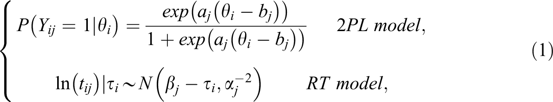
where

with the mean vector

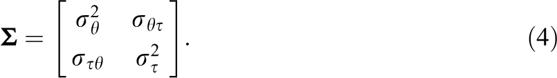
and the covariance matrix
For model identification,
The computation of residuals can be expressed as follows:

where the parameters in the equation have the same meaning as in Equation 1. These residuals have an approximate standard normal distribution because a larger negative value may indicate that the answer is given much quicker than expected. Thus, a response to an item is flagged as noneffortful when its residual is less than −1.645 (5% at the end of the left tail of a standard normal distribution). In our study, we refer to this method as the original standard residual (OSR) method.
Biased parameter estimates will lead to biased estimation of RT residual. We propose the following procedures to improve this method. First, accurate item parameter estimates should be obtained. Then, after removing noneffortful responses identified by OSR in each iteration, person parameter estimations are improved. These parameter estimates in turn can produce better residual estimates, which can be used to more accurately pinpoint the noneffortful responses. These procedures are explained in more detail as below.
Obtaining Accurate Item Parameter Estimates
Two different situations are considered here. For one, if item parameters are unknown, a mixture model method can be applied to improve item parameter estimation (Liu et al., 2020). First, based on both RA and RT, a mixture model is used to help differentiate noneffortful and effortful individuals (Liu et al., 2020). Once the effortful sample is identified, item parameter estimates can be obtained by using van der Linden’s (2007) hierarchical model to fit the data based on this sample. Liu et al.’s (2020) study showed that, compared to the item parameter estimates based on the whole sample, more accurate item parameter estimates can be obtained by the data consisted of effortful respondents. For details of this method, please refer to Liu et al. (2020). The Mplus code for the mixture model method is given in Appendix A in the online version of the journal. For another, if item parameters are known, they can be directly used in the following step.
Iteratively Purifying the Sample
When data sets are contaminated by noneffortful responses, the parameter estimates as well as RT residuals may be biased. On the contrary, when evaluated with parameter estimates that are closer to their true values, the RT residuals should be more capable to successfully identify outlier RTs. Hopefully, when aberrant responses are removed, the speed parameter (as well as the ability parameter) estimates will recover their true values better. The improved speed parameter estimates can in turn produce better RT residual results, which can be used to more accurately detect the noneffortful responses. Therefore, we propose the following iterative cleansing procedure (iterative conditional estimate standard residual method, ICSR):
When item parameters are unknown, use the pure sample
Fix item parameters as
Using
Fixed item parameter estimates as
Repeat Steps 3 and 4, until the proportion of responses that change classification (i.e., from effortful response to noneffortful response or vice versa) between two successive iterations does not exceed 0.001.
Upon convergence, the noneffortful responses identified in the last iteration are taken as the final detected noneffortful responses.
In each iteration, we compute a RT residual (based on Equation 5) for every response in the original full sample (given
If the above procedure simply stops at q = 0, RT residuals are calculated based on the speed parameter estimates obtained by conditional estimating with the fixed item parameters. Then, responses with residuals smaller than −1.645 are removed. We refer to this procedure as the noniterative conditional estimate standard residual (CSR) method.
Once the noneffortful responses are detected, they can be treated as missing values (i.e., the item is not answered by the examinee) to obtain a cleansed sample. For all the methods (i.e., OSR, CSR, ICSR), the final parameter estimates are estimated based on the resulting cleansed sample by fitting van der Linden’s (2007) hierarchical model. These estimates are hopefully less biased than the original parameter estimates based on the full, contaminated sample.
Simulation Studies
In this section, two simulation studies are conducted to evaluate whether the proposed method can successfully detect noneffortful responses and recover model parameters. In Simulation Study 1, item parameters are supposed to be unknown. Therefore, a mixture model method (Liu et al., 2020) is used to obtain item parameter estimates, which are fixed to apply both the iterative and noniterative procedures of RT residual-based methods. In Simulation Study 2, item parameters are supposed to be known.
Design
In order to investigate whether it was necessary to detect noneffortful responses, parameters were estimated based on the original full data set as a baseline to compare different methods in terms of parameter recovery. Specifically, in Simulation Study 1, the precision of the item parameter estimates based on the cleansed sample identified by the mixture model method is evaluated as well.
In Simulation Study 1, there were five manipulated factors: Noneffort prevalence ( Noneffort severity ( The difference between RTs of noneffortful and effortful responses ( Sample size (I) consisted of two levels: 1,000 and 2,000. Test length (J) consisted of two levels: 30 and 50. Note that when
In Simulation Study 2, the manipulated factors are the first three factors in Simulation Study 1 (i.e.,
Data Generation
For effortful responses, RA and RT were simulated from van der Linden’s (2007) hierarchical model (see Equations 1
–4). Item parameters were generated with
As for generating the noneffortful responses, first, we selected noneffortful test takers based on
Analysis
In Simulation Study 1, the mixture model method with the number of classes fixing at two for each latent variable (i.e., M22 in Liu et al.’s, 2020, study) was used to identify noneffortful individuals. van der Linden’s (2007) hierarchical model was calibrated using a Bayesian Gibbs sampling method during each iteration and to obtain the final parameter estimates. The data augmentation involves implementing a posterior sampler on the enlarged probability space for

where

Then, set k = k + 1 and repeat steps (b) and (c) until convergence is achieved.
In accordance with C. Wang, Xu, and Shang's (2018) study, the priors we chose for item parameters were
Criteria of Evaluation
Accuracy of identification of noneffortful responses
The true positive rate (TPR) and false discovery rate (FDR) of the identified noneffortful responses were computed and summarized over 30 replications. TPR was defined as the proportion of noneffortful responses that was correctly detected in the true noneffortful responses. It could be regarded as an evaluation of the power of these detecting methods. FDR was defined as the percentage of incorrectly detected noneffortful responses in the total detected noneffortful responses.
Parameter recovery
As the whole sample with detected noneffortful responses being recoded as missing is used to fit van der Linden’s (2007) hierarchical model, there is no sample selection bias during calibration. The parameter recovery can be evaluated directly. Bias and root mean square error (RMSE) were computed for each parameter, according to Equations 8 and 9:


where
Then, the relative efficiency (RE) was computed as the ratio of the RMSE of parameter estimates achieved by one of the methods to that resulted from fitting a van der Linden’s (2007) hierarchical model to the whole data set (RE1) or to that based on the pure sample identified by the mixture model method (RE2). RE2 was only computed for item parameters in IRT model. A value smaller than 1 implied an error reduction by using the detection method, while a value larger than or equal to 1 suggested using the more sophisticated method did not pay off or even obtain worse estimation.
Moreover, in Simulation Study 1, as the accuracy of the fixed item parameters was crucial for ICSR and CSR, we evaluated the accuracy of item parameter estimates calibrated based on the pure sample identified by the mixture model method (the estimates based on the original sample was set as the baseline). For the two-parameter logistic (2PL) model, the person parameters of the identified effortful group were scaled to a bivariate normal distribution during calibration, whereas for the generated data, the whole population followed a bivariate normal distribution. Therefore, a linking procedure was needed to adjust sample selection bias before direct comparisons could be made about item parameters. Accordingly, for the 2PL model, the estimates of item parameters were equated to the scale of true values based on a mean/sigma method (Kolen & Brennan, 2004) before bias and RMSE were computed. For the RT model, as data were generated based on the assumption that low-speed examinees were more likely to guess, the distribution of speed parameters of the effortful group might be different from standard normal distribution as well. We are not aware of any linking procedure to adjust the difference of scales of RT model parameter estimates. Therefore, the correlation of the estimated item parameters and their true values in the RT model is computed as an evaluation criterion. In addition, the consistency of residuals based on the estimated parameters in the RT model (estimated residuals) and those based on the true values (true residuals) is evaluated. It was assumed that, if the parameter estimates cannot recover the generated values well, the correlation between the estimated residuals and the true residuals should be low. This index (re ) could be calculated across items and replications by using a Fisher z-transformation, as seen in Equation 10.

where
Person fit
The percentage of misfit respondents, which is computed based on person-fit index, is used to evaluate whether the proposed method improves the person fit. The specific steps are as follows: First, noneffortful responses detected by OSR, CSR, and ICSR are recoded as missing. Second, van der Linden’s (2007) hierarchical model is fitted to the three cleansed data sets and the original full data. Third, based on the parameter estimates in the 2PL model, the corrected standardized log-likelihood person-fit index
Results
Simulation Study 1
According to Gelman and Rubin’s (1992) statistic, when van der Linden’s (2007) hierarchical model is calibrated, the Gibbs sampler successfully converged within 5,000 iterations (with the first 2,500 as burn-in). The results of convergence diagnostic statistics lead to the same conclusion for all our simulation studies and empirical example.
As the difference among all the methods is similar across different sample size and test length, we have focused on the results when I = 2,000 and J = 30 in this section. The results under different sample size and test length can be found in Online Appendix B.
As the purpose of applying the mixture model method is to improve item parameter estimation, we first examine the accuracy of item parameters that need to be fixed. As can be seen in Table 1, when all the items are assumed to be responded effortfully, although the RMSE under the mixture model method is higher than that based on the original data, the magnitude is small. For the RT model, re
is equal for both methods. The results suggest that when there are no noneffortful responses, the mixture model method can provide item parameter estimates almost as accurate as those based on the full data. When data are contaminated by noneffortful responses, the item parameters in the IRT model for both methods are recovered precisely when
Parameter Recovery for the Fixed Item Parameters in Simulation Study 1
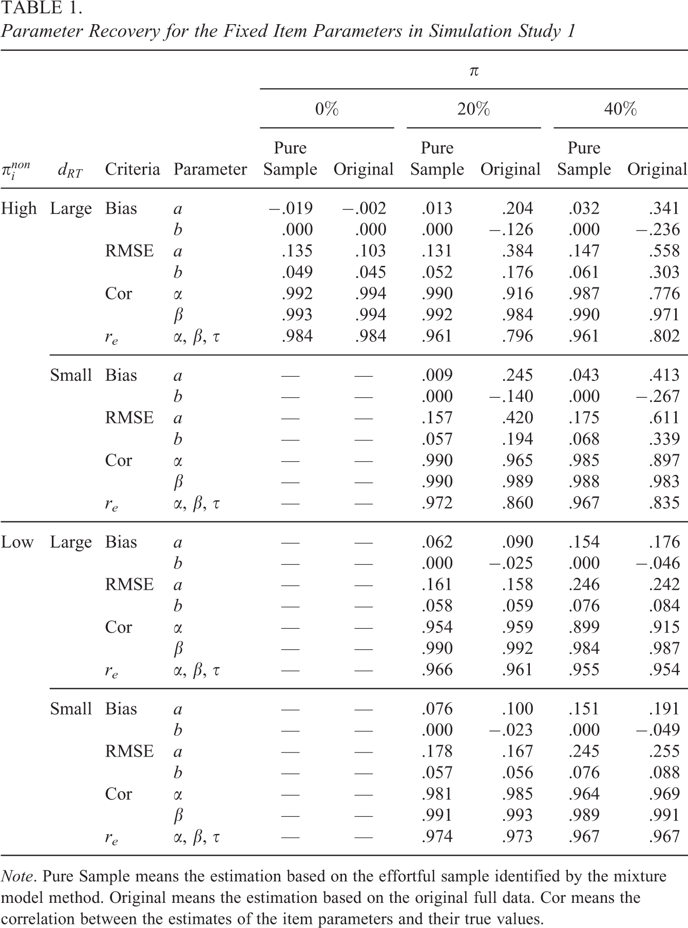
Note. Pure Sample means the estimation based on the effortful sample identified by the mixture model method. Original means the estimation based on the original full data. Cor means the correlation between the estimates of the item parameters and their true values.
The number of iterations under ICSR is summarized in Table 2. The higher level of noneffort severity requires more iterations before convergence is achieved.
Number of Iterations Under ICSR in Simulation Study 1

Note. ICSR = iterative conditional estimate standard residual method.
Table 3 summarizes the average TPR and FDR for noneffortful responses for all the three methods. In the condition that all the responses are effortful, TPR cannot be calculated and FDR is always 1. We computed the false positive rate (FPR, similar to Type I error in this situation) instead, which was defined as the percentage of responses incorrectly flagged as noneffortful in all the responses. The FPR for OSR and CSR are 0.047 and 0.048, respectively, which are both close to the nominal level (0.05). The FPR for ICSR is slightly inflated (0.060). The proportions of “pure sample” are about 95% for these methods. For each condition, the proportion of detected noneffortful responses are presented as well. First of all, when
Note that as noneffortful responses may have serious consequences for parameters estimation, in our study, higher TPR is stronger related to better estimation than lower FDR. As clearly shown in this table, compared to OSR, ICSR (as well as CSR) can increase TPR markedly when
Summary of the TPR and FDR of Three Methods in Simulation Study 1
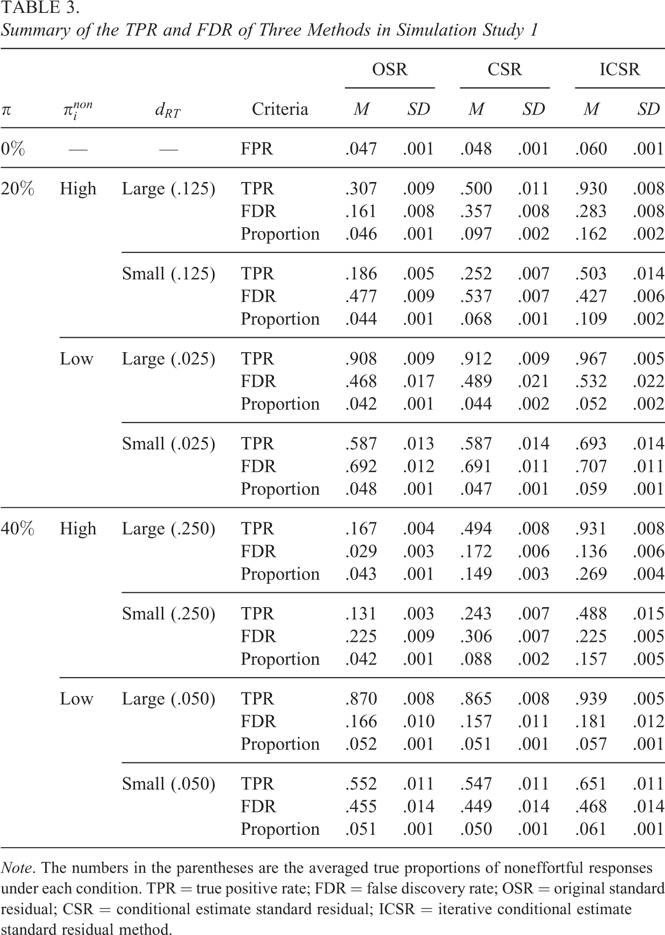
Note. The numbers in the parentheses are the averaged true proportions of noneffortful responses under each condition. TPR = true positive rate; FDR = false discovery rate; OSR = original standard residual; CSR = conditional estimate standard residual; ICSR = iterative conditional estimate standard residual method.
The intercoder reliability between these methods can be found in Table 4. As can be seen in this table, the detections by OSR and CSR, and CSR and ICSR are more consistent than those by OSR and ICSR. All the methods tend to show less consistency when
Summary of the Classification Consistency of Three Methods in Simulation Study 1
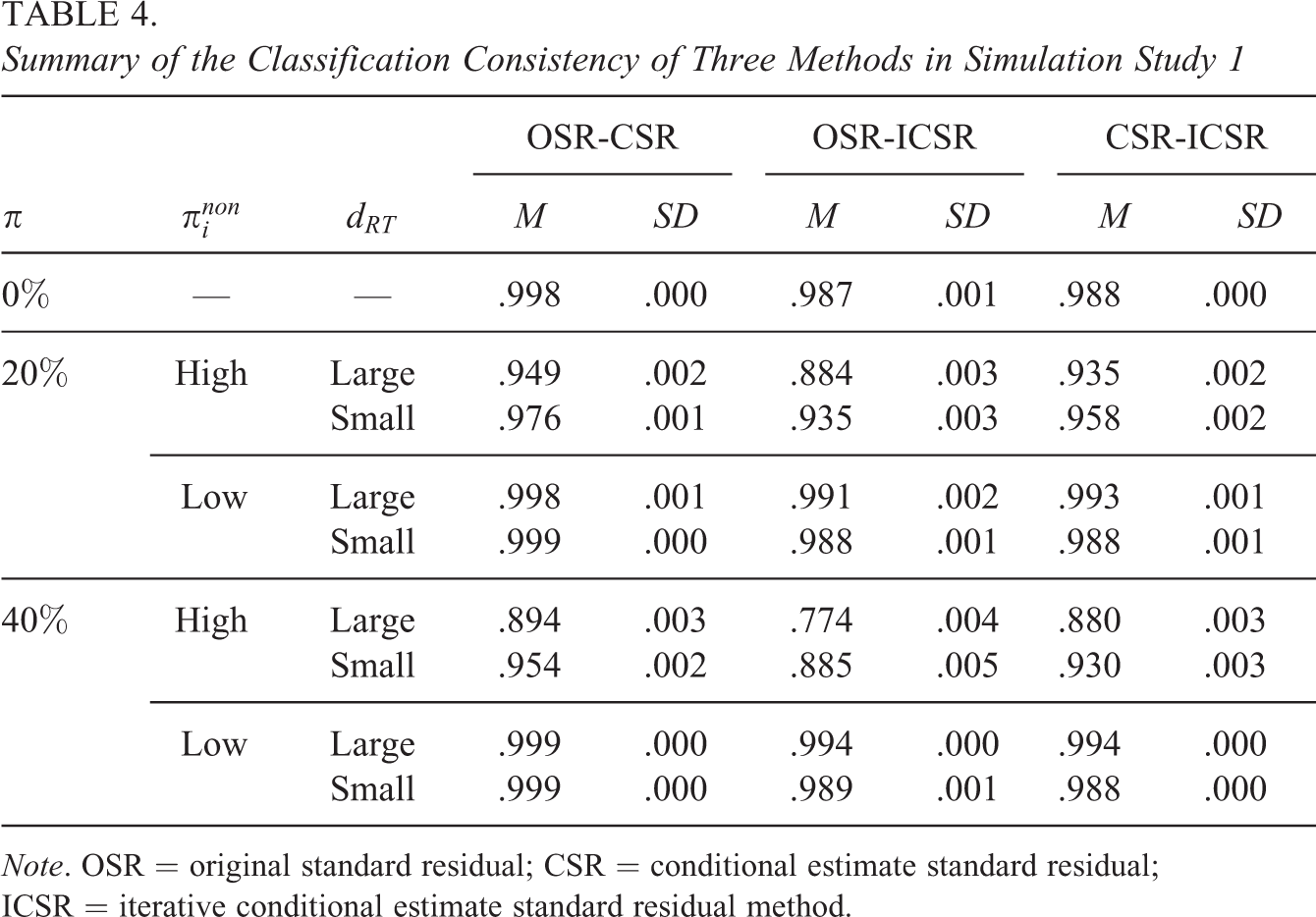
Note. OSR = original standard residual; CSR = conditional estimate standard residual; ICSR = iterative conditional estimate standard residual method.
A natural question that follows is how the performance of the proposed method in detecting noneffortful responses translates to parameter recovery. When
Parameter Recovery for All the Parameters When
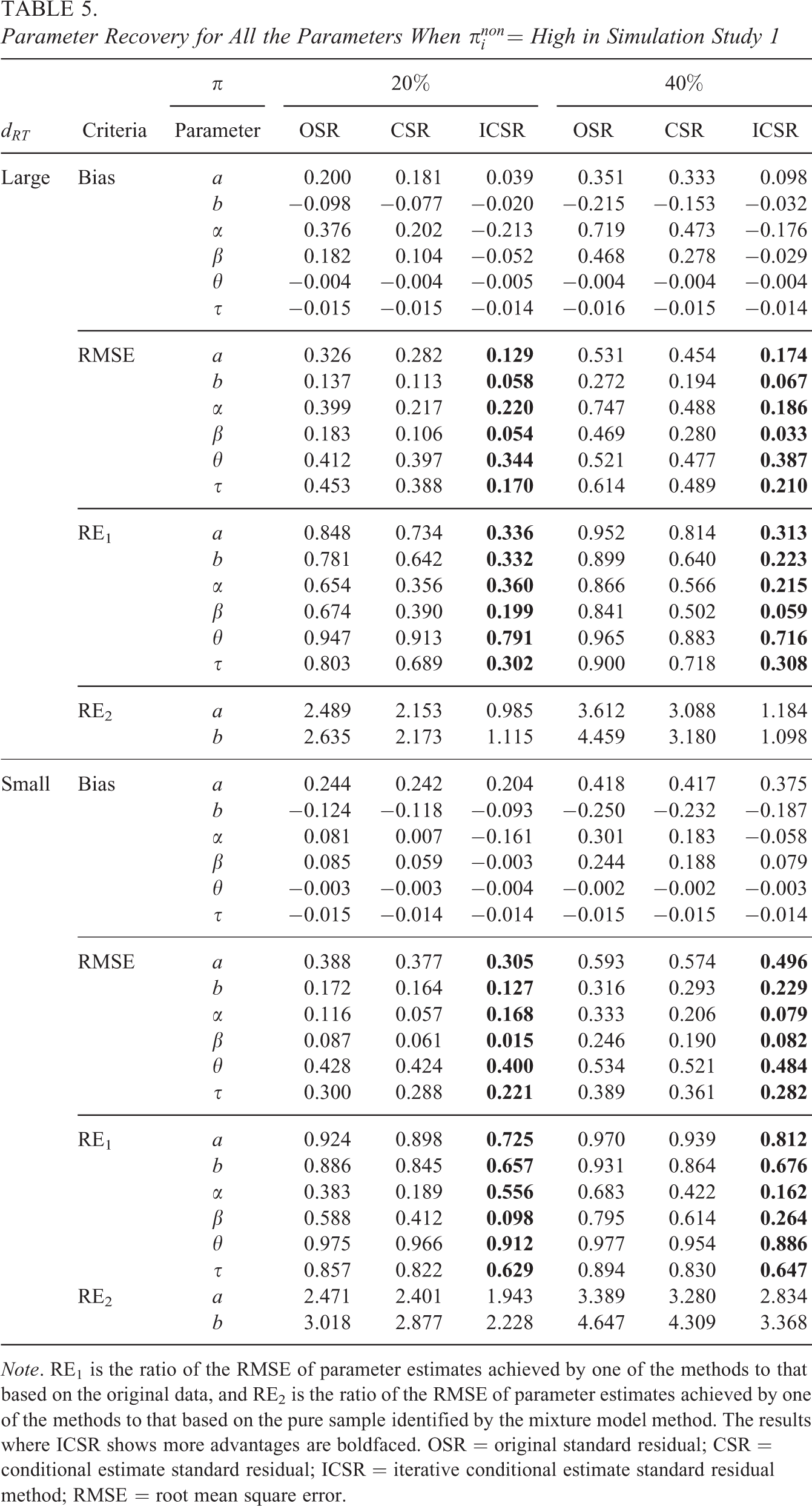
Note. RE1 is the ratio of the RMSE of parameter estimates achieved by one of the methods to that based on the original data, and RE2 is the ratio of the RMSE of parameter estimates achieved by one of the methods to that based on the pure sample identified by the mixture model method. The results where ICSR shows more advantages are boldfaced. OSR = original standard residual; CSR = conditional estimate standard residual; ICSR = iterative conditional estimate standard residual method; RMSE = root mean square error.
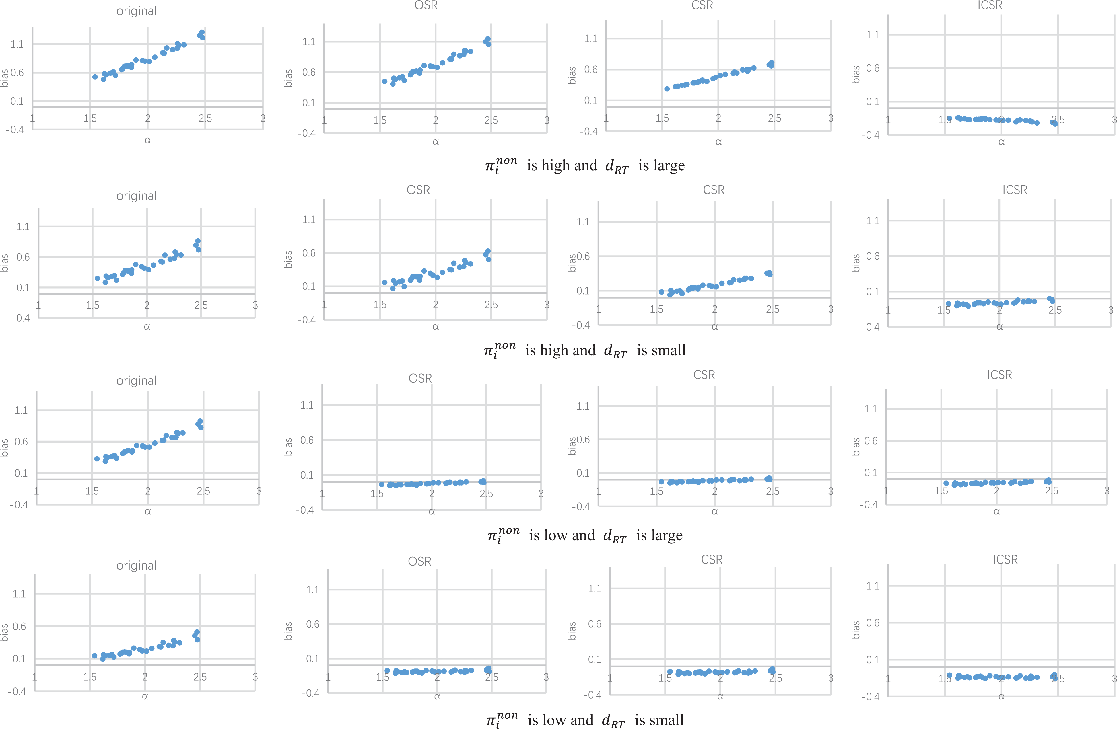
To better compare the bias for item parameters under different methods, Figures 1
through 6 show the item/person parameter bias of each item/person when
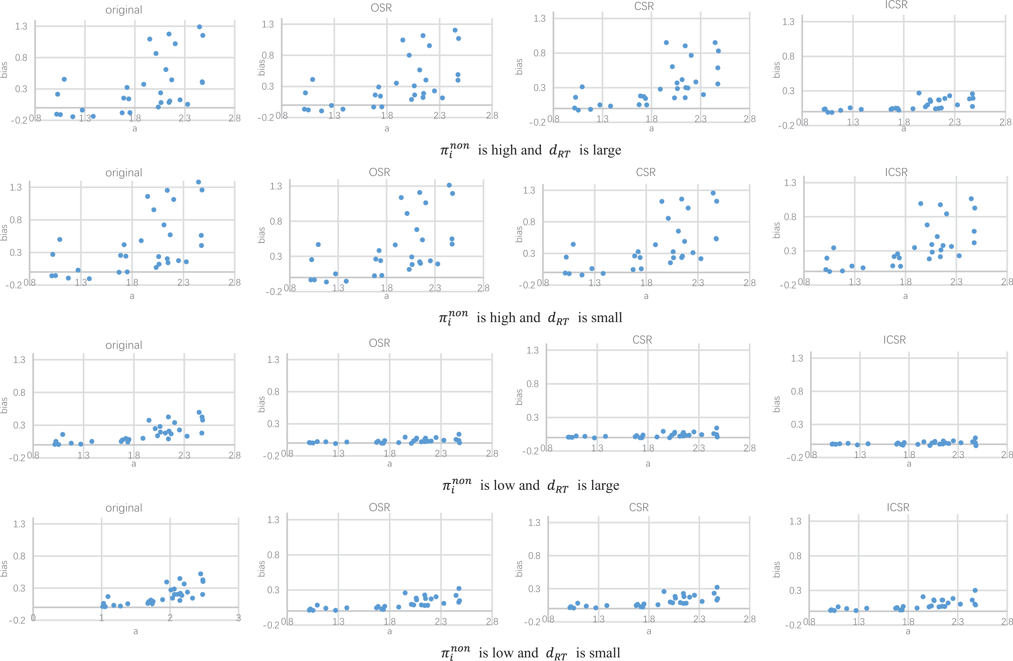
Bias of discrimination parameter estimates (when π = 40%).
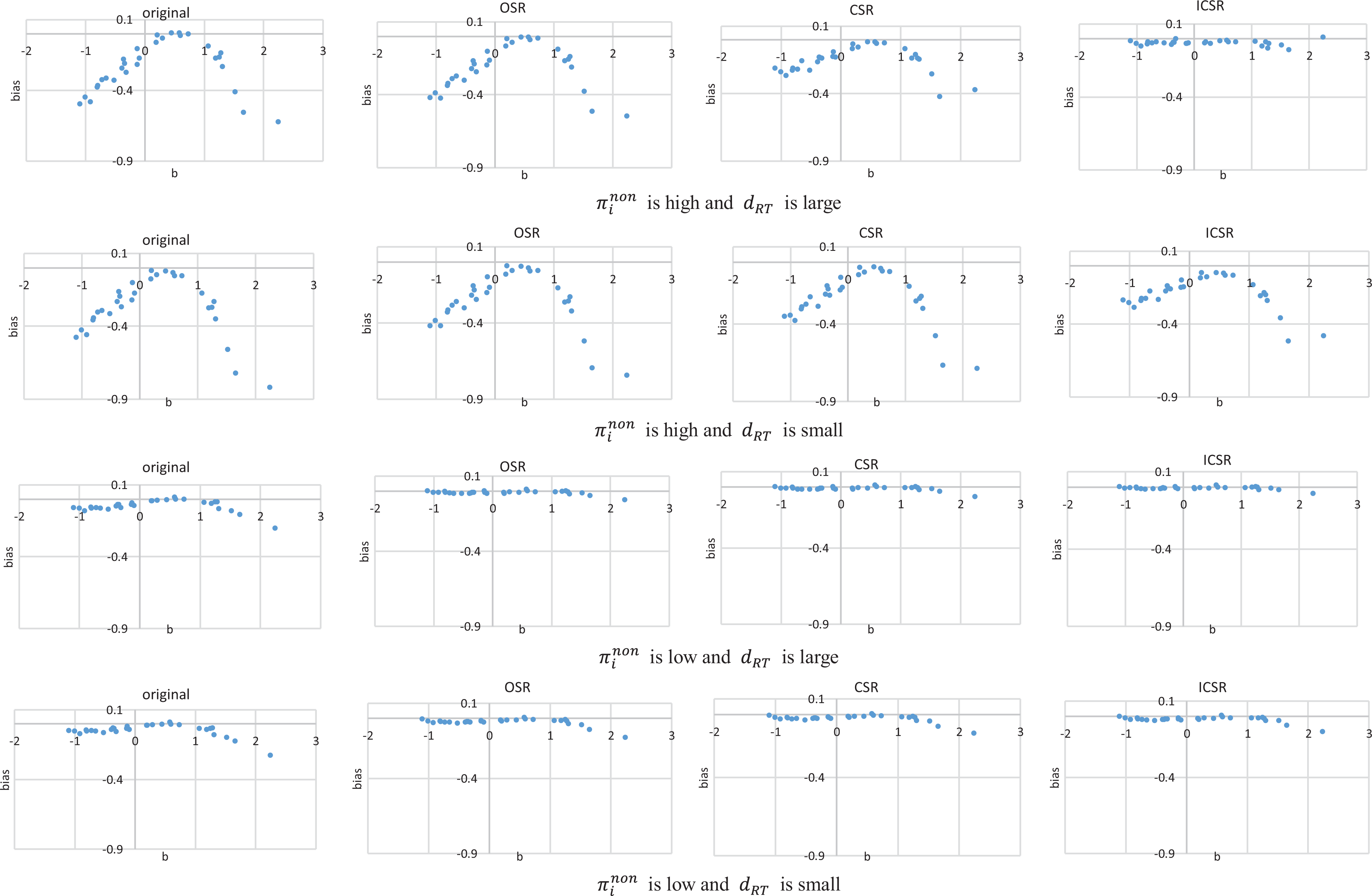
Bias of difficulty parameter estimates (when π = 40%).
Bias of time discrimination power parameter estimates (when π = 40%).

Bias of time-intensity parameter estimates (when π = 40%).

Bias of ability parameter estimates (when π = 40%).
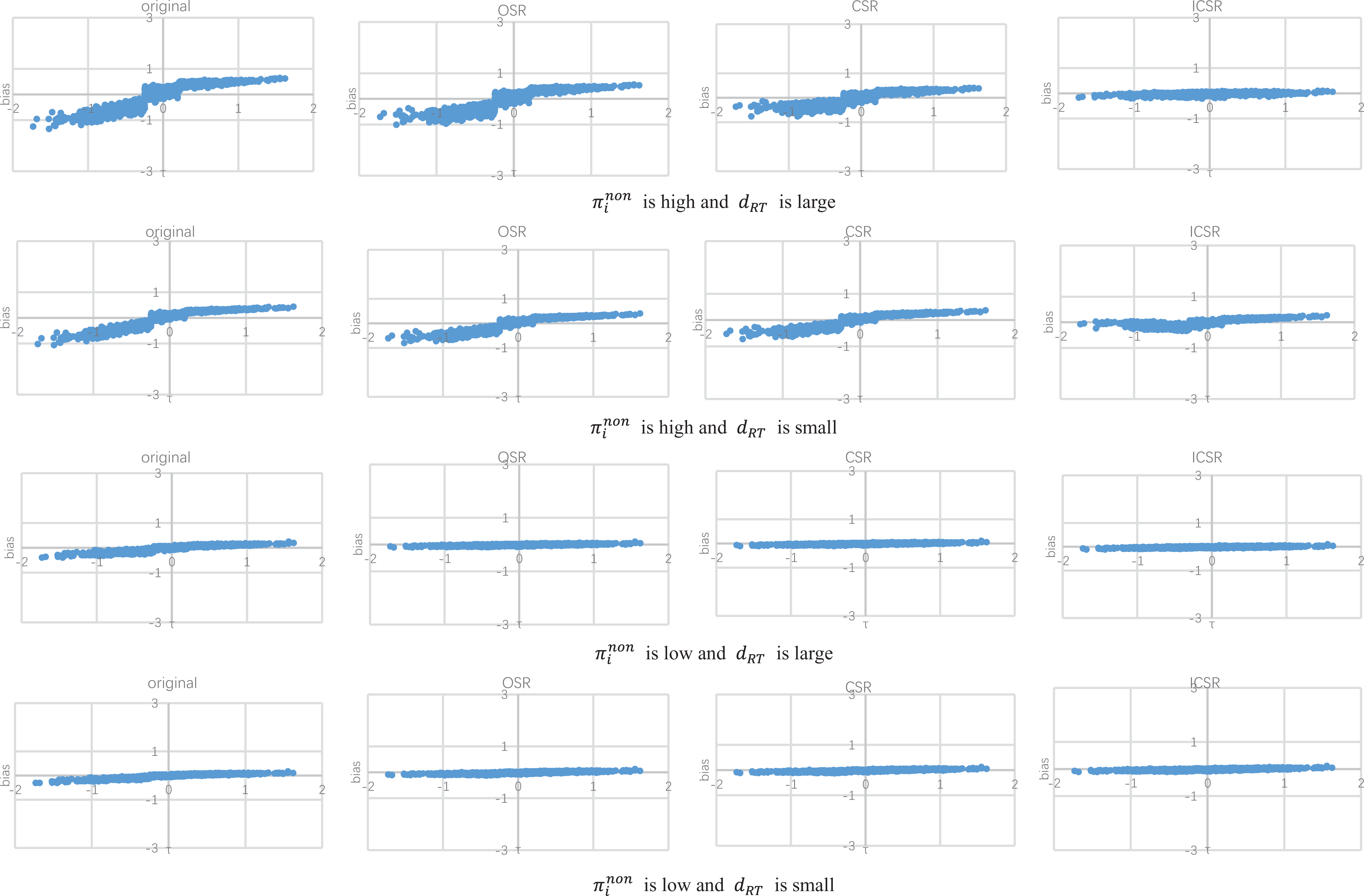
Bias of speed parameter estimates (when π = 40%).
Finally, the percentage of misfit respondents under each method and the original full data are summarized in Table 6. As can be seen in this table, when
The Percentage of Misfit Persons for Each Method and the Original Data (%)
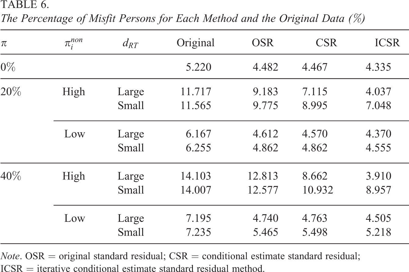
Note. OSR = original standard residual; CSR = conditional estimate standard residual; ICSR = iterative conditional estimate standard residual method.
Simulation Study 2
Given that in Simulation Study 1, the results under the conditions of
The classification consistency of these methods in Simulation Study 2 can be found in Online Appendix D. Similar to the results in Table 4, when
Summary of the TPR and FDR of Three Methods in Simulation Study 2
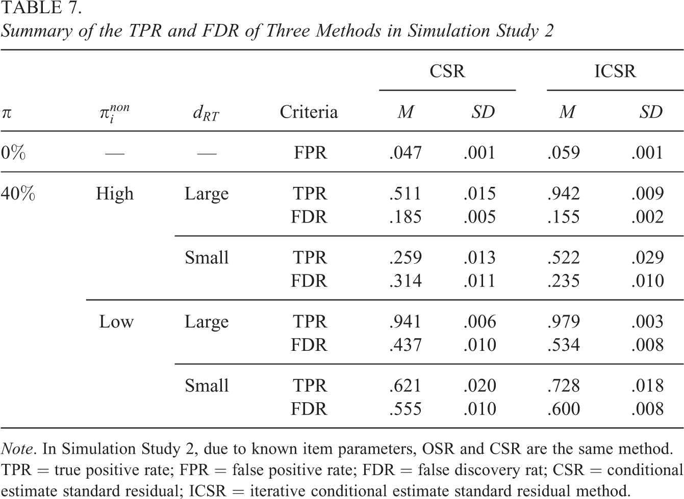
Note. In Simulation Study 2, due to known item parameters, OSR and CSR are the same method. TPR = true positive rate; FPR = false positive rate; FDR = false discovery rat; CSR = conditional estimate standard residual; ICSR = iterative conditional estimate standard residual method.
Table 8 shows the results of person parameter recovery across different simulation conditions in Simulation Study 2. Similar to the results in Simulation Study 1, when
Parameter Recovery for All the Parameters in Simulation Study 2
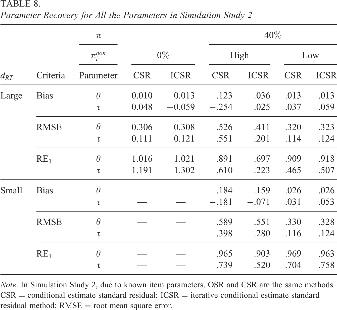
Note. In Simulation Study 2, due to known item parameters, OSR and CSR are the same methods. CSR = conditional estimate standard residual; ICSR = iterative conditional estimate standard residual method; RMSE = root mean square error.
Empirical Example
In addition to the simulation studies, the OSR, CSR, and the proposed method were used for the analysis of a real data set from Program for International Student Assessment (PISA) 2015. A sample of students taking two mathematics clusters from booklet 45 was selected as an illustrative example. As the RT might not be comparable across different languages/countries, we selected a subsample from Spain for analysis, which contained 901 participants in total. The selected data set included RA and RT information regarding 23 mathematics items, where 22 of them had two score categories and one of them had three score categories. For simplicity, Categories 2 and 3 were combined for the only item with three response categories so that all the items had two categories. In that way, van der Linden’s (2007) hierarchical model could be fitted. The percentage of missing values for RA is 7.42% while that for RT is 3.67%. The percentage of responses missing in RA and RT simultaneously is 3.62% (one response had RA information but no RT information). More details about the test design and sampling procedure can be found in the PISA 2015 technical report (Organization for Economic Cooperation and Development, 2017).
The original sample was used to estimate item and person parameters using van der Linden’s (2007) hierarchical model. Then, item parameters were obtained based on the effortful sample identified by the mixture model method. Once we got these parameter estimates, CSR, ICSR, and OSR were applied. The prior distribution, the initial values of each parameter, the number of chains, the number of iterations, the number of burn-in, and the thinning rate were set the same as in simulation studies. The iterative cleansing procedure converged in five cycles. For OSR, CSR, and ICSR, the percentages of flagged responses are 5.39%, 6.73%, and 8.48%, respectively, while the difference between RTs of noneffortful and effortful responses is 2.24, 2.04, and 1.88 for OSR, CSR, and ICSR, respectively. Therefore, this is similar to that when
Item parameter estimates based on the full sample and the samples cleansed by OSR, CSR, and ICSR are presented in Online Appendix E. As can be seen in that table, the results of the empirical data analysis are consistent with the findings of the simulation studies. First, cleansing the sample by these methods, especially by CSR or ICSR, results in noticeable increases in the time discrimination power estimates (see Figure 3 as a similar pattern in the simulation study). Second, the estimates of time-intensity parameter based on the sample cleansed by any method are higher than those based on the original sample. ICSR results in the highest estimates, which is consistent with the pattern in Figure 4 as well. Third, these methods barely have effects on the estimation of the discrimination parameter or difficulty parameter. This may be attributed to the fact that the proportion of noneffortful responses in these data may be rather low.
By regarding the estimates from the original full data as the baseline, we computed the relative difference (RD) and mean absolute difference (MAD) of the estimates based on different methods. RD is computed as the averaged difference between the estimates based on one of the detection methods and those based on the original data. MAD is computed as the averaged absolute difference between the estimates based on one of the detection methods and those based on the original data. The results are shown in Table 9. The RD and MAD of discrimination parameter and difficulty parameter are small for all the methods, which means that the item parameter estimates in the IRT model barely change after data are cleansed. All the methods tend to produce positive RD of both time discrimination power parameter and time-intensity parameter, with ICSR showing the largest difference from the original data. Although there is almost no RD for person parameters, the magnitude of MAD shows that there are some nonignorable differences between the person parameter estimates based on the original data and those based on the data cleansed by ICSR.
The RD and MAD of Parameter Estimates Compared to Those Based on the Original Data
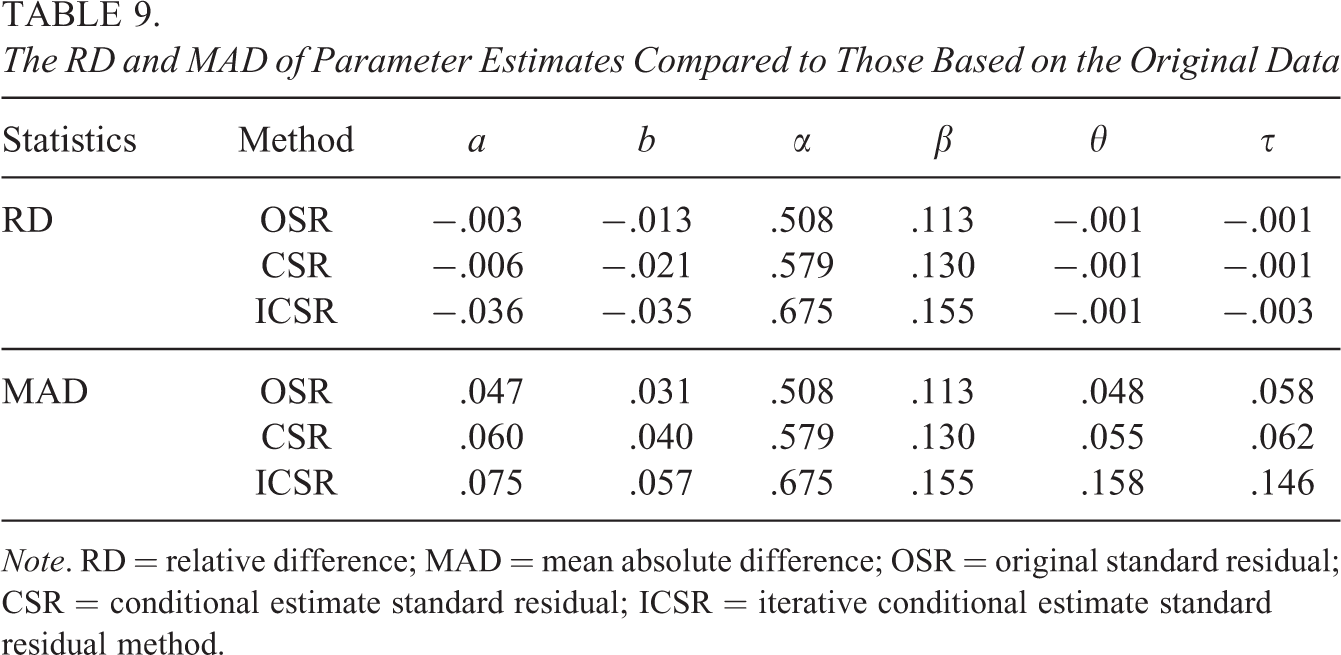
Note. RD = relative difference; MAD = mean absolute difference; OSR = original standard residual; CSR = conditional estimate standard residual; ICSR = iterative conditional estimate standard residual method.
Finally, in the real data analysis, the percentages of misfit respondents based on the original data, OSR, CSR, and ICSR are 3.885%, 2.886%, 2.664%, and 2.442%, respectively. ICSR improves the fit of the 2PL model slightly.
Discussion and Conclusion
In order to detect noneffortful responses, we propose a method based on RT residual analysis: the ICSR. This method is implemented with fixed item parameters and iteratively updates the person parameter estimates before calculating RT residuals. The proposed method is compared with a noniterative method with fixed item parameters (CSR) and an OSR in two simulation studies. Three factors related to noneffortful responses are focused on in the simulated studies: noneffort prevalence, noneffort severity, and the difference between RTs of noneffortful and effortful responses. We find that the proposed method is much more effective in detecting noneffortful responses and reducing the bias of parameter estimates when noneffort severity is high and the difference between RTs of noneffortful and effortful responses is large.
The proposed method is a kind of RT residual-based methods. These methods may show some advantages in the following aspects (Qian et al., 2016; van der Linden & Guo, 2008; C. Wang, Xu, & Shang, 2018). First, they have theoretical reference distributions of RT residual (i.e., standard normal distribution). Second, they make no assumptions concerning the form of irregular behavior, which means that neither RT nor RA of two different responses needs to be fitted by a specific model. Third, the residual-based methods can be applied easily to large-scale tests as they do not rely on visual inspection of RT distribution for each item. Fourth, these methods can be implemented when RT of all the responses does not follow a bimodal distribution. Finally, they can be used for items with different types, as they do not need to define the accuracy of random level (as Guo et al., 2016, did in their study for multiple-choice items).
When data are contaminated by noneffortful responses severely, to improve the performance of OSR, we need to obtain more accurate parameter estimates to calculate the residuals. To achieve this goal, we have applied two strategies in our proposed method. For item parameter estimation, when they are unknown, we first select a pure effortful sample by the mixture model method and find that the estimation is improved based on this effortful sample. When they are known before detection (e.g., de la Torre & Deng, 2008), estimation errors of item parameters are not considered. These item parameter estimates could be fixed in the following iteration steps. For person parameter estimation, we observe the performance gain in parameter recovery after iteratively removing noneffortful responses that may lead to biased estimates.
Obtaining accurate item parameter estimates is a crucial strategy for the proposed method. To begin with the unknown item parameter estimates, we have fixed item parameter estimates that are obtained by using the full data to fit the hierarchical model and applied the purification process (the method is called ICSR with original item parameter estimates, ICSRO). ICSRO is applied to the generated data of Simulation Study 1. The results show that when
Afterward, item parameters should be fixed in the purification process. As we have introduced before, Patton et al.’s (2019) iterative method suffers from convergence issues. This may be due to the fact that in their study, all the parameters need to be reestimated during each iteration, which leads to a big change of classification based on the renewed parameters. We hope to solve the convergence problem by fixing the item parameter estimates (i.e., not updating item parameter estimates for each iteration). Consequently, even with a more stringent convergence criteria than Patton et al.’s (0.001 vs. 0.01), all the replications of the proposed ICSR method have converged successfully in our study.
The strategy of iterative purification has been applied in educational and psychological measurement for a long time. For example, scale purification procedures have been strongly advocated and widely implemented onto IRT-based differential item functioning (DIF) detection methods (Candell & Drasgow, 1988; Lord, 1980; Park & Lautenschlager, 1990; W. C. Wang et al., 2009) and non-IRT-based methods (French & Maller, 2007; Holland & Thayer, 1988). Many researchers have found that, when tests contain less than 20% DIF items, DIF detection methods with scale purification outperform those without scale purification in reducing inflated FPRs and increasing deflated TPRs (French & Maller, 2007; Hidalgo-Montesinos & Gómez-Benito, 2003; C. W. Wang & Su, 2004). As data contaminated by aberrant responses (e.g., noneffortful responses) are similar to tests contaminated by DIF items, it is natural to apply the iterative purification process in detecting aberrant responses. de la Torre and Deng (2008) have proposed a method for improving the performance of the standardized log-likelihood person-fit statistic (lz ) by constructing the distribution for each lz through resampling methods iteratively. Their study shows that the proposed method has Type I error rates close to the nominal level for most ability levels and reasonably good power. Recently, Patton et al. (2019) have proposed to iteratively detect careless respondents and cleanse the data by removing their responses, which shows high-power and nominal-level FPR. However, these methods are based on person-fit statistics, and therefore, the classifications are only on the examinee level. As our method is based on a residual analysis, the classification results are for each item by person encounter, which can provide more detailed information than the person-level detections. Moreover, Patton et al. (2019) take the most recent set of parameter estimates as the final values after convergence, and we reestimate all the parameters based on the cleansed sample after convergence. These estimates are hopefully more accurate than theirs.
As noneffortful responses are characterized as responses with lower RA and RT, when noneffort severity is high, the estimation based on the full sample or data cleansed by OSR will obtain biased item parameters, while ICSR, sometimes CSR in this article, can eliminate the bias to some extent. First, the estimation based on the original data and OSR tends to underestimate discrimination parameters, especially for items with higher true values of discrimination parameters. In these situations, including noneffortful responses to fit the model may reduce the information provided by the data, as the noneffortful responses exhibit much less or even misleading psychometric information (Wise, 2017). Second, fitting van der Linden’s (2007) hierarchical model to the original data or OSR will overestimate the difficulty parameters for both easy and hard items, which means that these items seem more difficult than they really are. It may be due to the fact that RA is much lower by noneffortful responding. Third, the estimation based on the original data and OSR produces large positive bias of time discrimination power parameters for items with larger true α values. As can be seen from Equation 1, items with lower time discrimination power may distinguish fast and slow respondents worse. As deleting noneffortful responses by the proposed method means deleting responses with extreme low RTs, which bring nuisances unrelated to the respondent’s true speed, these methods lead to an increase of α. Fourth, the time-intensity parameter estimates based on the original data or OSR are generally underestimated. As can be seen from Equation 1, items with lower time intensity require less time to complete. Therefore, removing noneffortful responses with lower RT to a certain item can markedly increase the RT needed by the item in general. Finally, the ability parameter estimates based on the original data or OSR are overestimated for low-ability examinees and underestimated for high-ability examinees. It may be caused by the fact that the accuracy of noneffortful responses is 0.25 regardless of examinees’ ability level. Therefore, low-ability examinees perform better, whereas high-ability examinees perform worse than they really are. The speed parameter estimates based on the original data or OSR are overestimated for slow examinees. This is related to the assumption in our simulation studies, where slow examinees are more likely to respond noneffortfully. These noneffortful responses of slow examinees present extremely small RT, which leads to relatively larger estimates of speed parameters.
There are many important applications of parameters in van der Linden’s (2007) hierarchical model, and they all can be adversely affected by miscalibrated parameters due to noneffortful responses. Our proposed method provides a way to efficiently detect noneffortful responses and improve parameter estimation. For example, as high discriminating items are quite desired in item selection, the proposed method can avoid erroneously neglecting these items in item selection because they can avoid underestimation of discrimination parameters. Moreover, Choe et al. (2018) have proposed a novel item selection criterion that maximizes Fisher information per unit of expected RT. One of their methods favors items with high information and low expected RT. As items with low β tend to have low expected RT, it is obvious that the proposed method can obtain less biased β estimates in some situations, which will lead to more accurate expected RT. In summary, we highly recommend practitioners to detect noneffortful responses before estimating item parameters.
Furthermore, our study has some limitations and can be extended in the following ways. First, in this study, data are generated assuming that slow examinees were more likely to guess. In practice, noneffortful responding may be irrelevant to examinees’ ability or speed (e.g., Sundre & Wise, 2003; Wise & DeMars, 2005; Wise & Kong, 2005). In accordance with that, future studies can draw noneffortful samples randomly from the whole sample. Second, the iterative purification process with fixed item parameters can be applied in detecting other forms of aberrant responses (e.g., cheating, items with preknowledge) based on other statistics (e.g., person-fit statistics, nonparametric statistics). Third, the current study adopts a mixture model method with a fixed number of latent classes to classify the noneffortful and effortful groups. Other methods can be developed to select a pure group to obtain more accurate item parameter estimates. Fourth, the iterative purification process is quite complex and time-consuming. The results in our simulation studies show that when noneffort severity is low, the iterative process does not bring much improvement for identification accuracy and parameter recovery. In real data analysis, practitioners should decide whether it is necessary to use the proposed iterative method. In order to have a deeper understanding of this method, future studies would compare the proposed method with other within-subject mixture approaches (e.g., Kuijpers et al., 2020; Molenaar et al., 2018) in various conditions. Fifth, as can be seen from the results, the proposed method may increase estimation error in the RT model, especially for time discrimination parameter. This may be due to the fact that deleting extremely fast responses changes the distribution of RT. Maybe some robust estimation methods (e.g., see Hong & Cheng, 2019) that down-weight flagged response patterns can provide an alternative to directly removing noneffortful responses (i.e., as we did in our current study). Finally, due to the “masking effect,” we caution readers against overgeneralizing the results of the current study to the situation where noneffortful severity is extremely high (e.g., almost all the responses of a respondent are noneffortful). A large-scale simulation study is needed in the future to explore the performance of the proposed method in such extreme situations.
Supplemental Material
Supplemental Material, sj-docx-1-jeb-10.3102_1076998621994366 - Detecting Noneffortful Responses Based on a Residual Method Using an Iterative Purification Process
Supplemental Material, sj-docx-1-jeb-10.3102_1076998621994366 for Detecting Noneffortful Responses Based on a Residual Method Using an Iterative Purification Process by Yue Liu and Hongyun Liu in Journal of Educational and Behavioral Statistics
Footnotes
Declaration of Conflicting Interests
The author(s) declared no potential conflicts of interest with respect to the research, authorship, and/or publication of this article.
Funding
The author(s) disclosed receipt of the following financial support for the research, authorship, and/or publication of this article: This research is supported by the Grant from National Education Examinations Authority of P. R. China (GJK2017015).
References
Supplementary Material
Please find the following supplemental material available below.
For Open Access articles published under a Creative Commons License, all supplemental material carries the same license as the article it is associated with.
For non-Open Access articles published, all supplemental material carries a non-exclusive license, and permission requests for re-use of supplemental material or any part of supplemental material shall be sent directly to the copyright owner as specified in the copyright notice associated with the article.