




Abstract
A Monte Carlo simulation was performed to compare methods for handling missing data in growth mixture models. The methods considered in the current study were (a) a fully Bayesian approach using a Gibbs sampler, (b) full information maximum likelihood using the expectation–maximization algorithm, (c) multiple imputation, (d) a two-stage multiple imputation method, and (e) listwise deletion. Of the five methods, it was found that the Bayesian approach and two-stage multiple imputation methods generally produce less biased parameter estimates compared to maximum likelihood or single imputation methods, although key differences were observed. Similarities and disparities among methods are highlighted and general recommendations articulated.
In longitudinal data analytic settings, direct applications (Bauer, 2007; Harring & Hodis, 2016) of finite mixture models are commonplace in the empirical literature, in which the primary goal is to identify unobserved (latent) heterogeneous subpopulations of growth trajectories (Jung & Wickrama, 2007). As a hypothetical example, researchers may follow students’ self-concept of ability (SCA) in math scores over time and wish to identify which students in the sample are “constantly high” in SCA, “slow decliners” in SCA, or “rapid decliners” in SCA (Musu-Gillette et al., 2015). These subpopulations of students are latent and are not identified a priori like groups manifest in the data as observed categorical independent variables (e.g., gender, socioeconomic status, experimental condition). Instead, their existence must be inferred from unobserved clustering embedded in the growth patterns themselves. Growth mixture models (GMMs; Muthén, 2001; Muthén & Shedden, 1999) are commonly employed to model repeated measures data for investigating this type of population heterogeneity in individuals’ longitudinal profiles although other types of longitudinal mixture models exist (see, e.g., McNeish & Harring, 2020; Nagin, 1999).
The increased popularity of GMMs in recent years kindled a number of methodological studies that focused on issues pertaining to using the model under varying real-world conditions. Much of the methodological research has dealt with testing indices for data-model fit (Henson et al., 2007; Nylund et al., 2007), evaluating methods that help decide on the number of subgroups (Bauer & Curran, 2003; McNeish & Harring, 2017; Nylund et al., 2007; Tofighi & Enders, 2007), examining the classification accuracy of models (Enders & Tofighi, 2008; Peugh & Fan, 2012), comparing estimation methods for finite mixtures (Hipp & Bauer, 2006; McLachlan & Krishnan, 2007), or showing how differing settings other than the default settings in popular software for estimating these models can impact parameter recovery and precision (Li et al., 2014).
Despite the research made available to help inform and refine the use of GMMs, not much attention has been devoted to testing GMMs in the presence of missing data. In the social and behavioral sciences, missing data analysis merits special attention because repeated measures data used for fitting GMMs are typically rife with missing data due to various issues like data collection error, participant nonresponse to specific items, drop out, or failure to participate in at least one wave of data collection.
Studies on handling missing data in the context of GMMs recommend using full-information maximum likelihood (FI) over single-stage multiple imputation (MI; Enders, 2011; McLachlan & Peel, 2000; Sterba, 2016) because MI requires the grouping information to be known a priori in order to correctly impute data (Enders, 2010) for each group. Since the grouping information for mixture models is latent, the use of MI with mixture models is problematic. Failure to specify a grouping variable when using MI has been shown to produce biased parameter estimates and incorrect identification of classes (Enders, 2011; Sterba, 2016).
Some recent studies have also turned to Bayesian methods to estimate GMMs with missing data using Markov chain Monte Carlo (MCMC) algorithms such as the Gibbs sampler. In a simulation study by Depaoli (2013), parameter recovery for a three-class GMM was investigated under varying degrees of class separation, sample size (SS), class proportion, and method of analysis (FI vs. a fully Bayesian [FB] approach using different priors). It was shown that a Bayesian approach with informative priors produced less biased estimates of the means (slopes and intercepts) than when using maximum likelihood (ML) estimation, particularly when separation among classes was larger and SSs were modest. Parameter variances, however, were not well recovered under all conditions. One limitation of the study, however, was that missing data were not considered. Other studies such as those by Song and Lee (2002), Cai et al. (2010), and Lu et al. (2011) proposed using Bayesian methods to address missing data that were missing at random (MAR) when using GMMs, finding favorable outcomes to using such models.
Harel (2007, 2009) also suggested using a two-stage multiple imputation (2M) approach to remedy the problems of using single-stage MI with mixture models. The original idea proposed by Shen (2000) as a way to impute data of different types (Rubin, 2003; Schafer & Graham, 2002) was extended to the context of mixture regression models. According to Harel (2009), the 2M method allows unbiased parameter estimates that are similar to those obtained from FI estimation. Nevertheless, the extent to which the method will work and how well it will perform in the context of GMMs and the different conditions of missingness as compared to these other proposed approaches (FI, MI, and FB methods) is unclear.
Despite the vast methodological work done in the area of GMMs and missing data, no study has brought these methods together and compared their performance under varying conditions specific to GMMs and missing data. The purpose of this study is to fill this important gap in the literature by comparing different methods—those that have been suggested for handling missing data in the context of GMMs as well as those not yet extended to this longitudinal context.
To outline the structure of this article, we first overview the generic latent growth model (LGM) and demonstrate how it extends to GMMs. In a subsequent section, missing data and missingness mechanisms are outlined followed by a review of estimation methods used in the simulation. Details regarding the single and two-stage multiple imputation methods are also provided. We provide a Monte Carlo simulation study to highlight the performance of these methods across manipulated conditions thought to occur in practical research scenarios and those that have been shown to impact results in past GMM simulation studies. Specifically, we explore convergence, classification accuracy, relative bias of parameter estimates, and precision of the standard errors (SEs).
Overview of LGMs and GMMs
Latent Growth Models
Several options exist for analyzing data from longitudinal studies with a continuous repeatedly measured outcome. The latent curve model (McArdle, 1986; Meredith & Tisak, 1990), or more generally, LGM (see, e.g., Hancock et al., 2013), an important subclass within structural equation modeling (SEM), is commonly employed to analyze continuous repeated measures data of this type. Theoretically, this approach hypothesizes the existence of latent trajectories capturing an underlying change process that can only be observed indirectly via the repeated measures (Bollen & Curran, 2006). The LGM permits the correlational structure of the repeated measures to be separated into within-individual variability as well as between-individual variability in individual subjects’ growth characteristics across time (see, e.g., Preacher et al., 2008).
Consider the conventional linear LGM with r time-invariant covariates takes the form of a restricted confirmatory factor analytic model, such that


In Equation 1,
In Equation 2, individual linear growth factors are decomposed into the


where
Multiple group LGMs
Populations are often comprised of heterogeneous subpopulations that may follow different growth trajectories. These subpopulations can sometimes be identified by discrete covariates that are manifested in the population (e.g., gender, categorized age groups). In this case, parameters can be estimated separately for each group with what is referred to as a multiple-group model (e.g., Muthén & Curran, 1997), where Equations 1
–4 would be augmented with a g (
Growth Mixture Models
GMMs are a generalization of the multiple group modeling framework, in which group membership is latent and must be inferred via the characteristics of within-individual profiles (Muthén, 2001; Muthén & Shedden, 1999; Nagin, 1999). Instead of a known value for group membership, each observation receives a probability of membership in each of the estimated latent classes. Assuming multivariate normality, the composite probability density of a vector of continuous outcome variables,

where K (


with the assumptions that the residuals and random effects for individual i follow distinct multivariate normal distributions,


In sum, GMMs are a natural extension of LGMs that utilize a discrete latent variable with a specific number of categories permitting clusters of longitudinal change to be captured by distinctly parameterized growth trajectories. As McNeish and Harring (2020) point out, this discrete latent variable serves as a moderator for the whole (LGM) model, allowing parameter estimates to differ for the different categories of the discrete latent variable. Whether these latent classes are theorized a priori or whether they emerge from an exploration of the data, fitting GMMs to many longitudinal datasets can be severely hampered by the real possibility of the presence of missing data. This is discussed next.
Missing Data Mechanisms
Rubin (1976) regarded missing data as random variables with a probability distribution. Missing data were classified as having one of the three mechanisms: MAR, missing completely at random (MCAR), and missing not at random (MNAR). Briefly, for data that are MAR, the missingness is independent of the variable with missingness, but dependent on other observed variables. That is, if
Extended Ignorability
Harel (2003) and Harel (2009) extended the meaning of ignorability by decomposing the missing data into different types. If the missing data,

According to Rubin (1987), under the conventional MAR assumptions, imputations for any missing data can be drawn from

and

A weaker ignorability condition based on these relations that are pertinent to GMMs, where the missingness in the measured variables might be conditioned on the completely unobserved latent class variable (e.g., missing measured variable,

If the CMAR

which, under Rubin’s original assumptions of MAR, imputations can be drawn from
Several options are available for addressing missing data under the four assumptions of missingness just reviewed. These include listwise deletion (LD), FI, MI methods, and Bayesian estimation using MCMC. These are discussed in the context of previous research on finite mixture models followed by the research questions driving the simulation study.
Approaches for Addressing Missing Data
Like finite mixture models in other contexts, GMMs may be estimated using various approaches, but ML estimation via the expectation–maximization (EM) algorithm (Harring, 2012; Muthén & Shedden, 1999) and a Bayesian framework using MCMC methods (e.g., Depaoli, 2014; Kohli et al., 2015; Lock et al., 2018) seem to standout in the literature. These two methods are popular because they are able to handle latent, unobserved parameters that are part of the GMM model, as well as when the datasets contain missing observations. These methods have the capability to estimate parameters even with missing data under strict assumptions about the missingness. These methods are discussed briefly next.
FI via the EM Algorithm
Aside from being relied on for estimating parameters, FI estimation is widely accepted as a way to deal with missing data (FI; Dempster et al., 1977). In general, the essence of FI estimation is to use each individual’s complete data to find the parameters across individuals that maximize the likelihood function. As long as the missingness can be assumed to be MAR, the ML estimates can be found using the marginal probability of the individuals’ observed responses. In other words, FI uses any and all of the available data for each individual, without the need to alter any of the data, for example, by deletion or imputation. The actual derivation at a set of parameter estimates that maximize the likelihood is obtained through the EM algorithm (McLachlan & Peel, 2000). The EM algorithm alternates between an E-step and M-step to arrive at a solution that maximizes such a likelihood function with missing information. Dempster et al. (1977) demonstrated how this likelihood could be assumed to be similar to other missing data problems. Essentially, the likelihood can be rewritten with the assumption that the class parameter is observed and the maximization of the log-likelihood becomes conditional only on the observed data and candidates of these “observed” parameters. The E-step amounts to computing a posterior probability for each individual evaluated at current parameter values, and during the M-step, posterior probabilities from the E-step are used to maximize the conditional expectations by replacing the unknown class indicators as well as computing other model parameters. Then, these new parameters are carried over to the next iteration, where the back and forth mechanism continues until parameters and class proportions that maximize the likelihood are found based on certain convergence criteria (e.g., the difference in log-likelihood values between successive iterations is negligible).
FB via MCMC
A FB approach using an MCMC simulation technique is another possible approach for obtaining parameter estimates for the GMM (Asparouhov & Muthén, 2010; Gelman et al., 1995), which can also be implemented to handle missing data. Although there are a number of nuanced MCMC methods that have been developed, the Gibbs sampler is one of the more widely used methods (Geman & Geman, 1984; Muthén et al., 2010). Within the Gibbs sampler, a sequence of values for unknown parameters, latent variables, and missing observations are iteratively obtained in order to create posterior distributions for the unknown parameters and missing data variables. This is done by conditioning on the observed data and prior information and iteratively updating one parameter and missing value at a time. Parameters are continuously updated by conditioning on the priors and observed data but also on the values from each previous iteration. See Asparouhov and Muthén (2010) for a more comprehensive, step-by-step guide to the mechanics underlying the Gibbs sampler.
Multiple Imputation
As a way to retain the advantages of MI methods and model sources of uncertainty mentioned before, Rubin (1987) recommended using MI. MI fills in values for the missing data in three general steps. First, multiple complete datasets are created by the imputation of plausible values in the cells where missing data are present. Then, the multiple complete datasets are analyzed. Finally, the results from the multiple analyses are aggregated. The underrepresented uncertainty of parameter estimates is addressed by creating several versions of complete data that produce multiple parameter estimates. These estimates are then averaged to produce a final parameter estimate. Special rules derived by Rubin (1987) are applied in the aggregation stage of SEs to account for between imputation variance and within imputation variance.
Filling the missing data cells in the first step is typically the most crucial step of the process. Several imputation methods have been suggested, but in general, these methods can be classified into two frameworks: joint-modeling (Rubin, 1987) and fully conditional specification (van Buuren et al., 2006). While these two approaches are different in how they impute the missing data, they are both grounded in Bayesian methods, which entails specifying probability distribution functions (or PDFs) for the parameters of interest [typically referred to as the prior distributions, or simply prior(s)], specifying a likelihood function—a conditional PDF of the data given the parameters—that use the data to provide evidence about the parameters and creating a posterior distribution using the prior(s) and likelihood function to describe the distribution of the parameters in light of the data. The three elements are then brought together by Bayes’s theorem, which equates the posterior distribution as the product of the prior distribution and the likelihood function divided by the marginal distribution of the data.
Two-Stage MI
Another option for addressing the missing data problem in GMMs is the 2M approach introduced by Harel (2003). The 2M method is feasible on the assumption of extended ignorability. In the 2M method, m sets of

where

where
After analysis, the resulting
The 2M method has been mainly applied in situations where missing data can be thought of as being of distinct types of missingness, such as surveys containing planned and unplanned missing data (Graham et al., 2001; Rhemtulla & Hancock, 2016), longitudinal models with ignorable intermittent missing data points (Hedeker & Gibbons, 1997), and nonignorable dropout missing (Harel, 2003). The method has also been applied with latent variable models that involve analysis with missing data and unobserved latent variables, such as latent class regression models (Harel et al., 2013) and latent class contingency tables (Winship et al., 2002).
Although empirical studies have used the 2M method to address missing data, no studies to date have tested the use of the method through simulation, let alone on different conditions of missingness or GMMs. Thus, while the method has been theoretically justified and applied in several different scenarios, the extent to which the method will work and how well it will perform relative to other missing data handling methods, such as FI, MI, or FB methods remains ambiguous.
Purpose of the Study
The purpose of this study is to extend the use of the several existing methods presented to address the issue of missing data in the context of GMMs. A simulation study will be conducted to compare the FI, FB using Gibbs sampling, and the 2M approach. In typical GMM simulation studies, varying SSs, number of latent classes, and latent class separation are among the conditions explored. Other important considerations that have been the focus of studies on GMMs such as class enumeration and fit evaluation criteria (see, e.g., Bauer, 2007; Bauer & Curran, 2003) will not be considered in order to focus on the effects of missingness on parameter estimation. In typical missing data studies, these varying rates of missing data and missingness mechanism are some common conditions of interest, which will be explored in this study. Specifically, the current research will compare the performance of LD, FI, MI, 2M, and an FB approach for estimating GMMs when there are missing data at various occasions under varying conditions common in the GMM literature as well as different missing data conditions.
Specifically, the study will attempt to address the following. When the goal is to classify individuals into groups, for which method will the growth model provide the highest percentage of classification accuracy for varying rates of missing data, SS, class separation, and missingness mechanism? For what rate of missing data and class separations will the GMM produce biased parameter estimates when utilizing the different missing data handling methods under conditions of MAR (or CMAR Which missing data handling methods produce SE estimates that are most accurate? Are there any advantages to using any of the missing data handling methods in the context of GMMs? Particularly, is using a more complicated method worth the extra effort for producing unbiased parameter estimates?
To answer these questions, a Monte Carlo simulation study was conducted using the conditions that were mentioned previously.
Method
Simulation
A Monte Carlo simulation was used to compare LD, FI, MI, FB, and 2M for handling missing data in the context of GMMs. The study involved testing conditions that are known to impact the parameter recovery of the population parameters. These conditions include missingness mechanism, missing rate (MR), SS, and class separation.
Data generation
Data for four timepoints were generated from a two-class linear growth model with random intercepts and slopes corresponding to Equations 6 and 7. A two-group factor analytic model was parameterized such that the loadings were fixed to model linear growth with four timepoints. The number of classes was chosen and kept fixed in order to keep the study focused on the missing data handling issue. The motivation for the number of timepoints came from recommendations by Muthén and Curran (1997), as well as past studies justifying this number (see, e.g., Depaoli, 2013; Tueller & Lubke, 2010). Data sets consisting of SSs of 100, 200, 500, and 1000 with an equal number of observations in each of the two classes were used and chosen based on these previous studies.
The means of the latent growth factors for the two classes were manipulated to achieve varying degrees of class separation using the Mahalanobis distance (MD), a measure of separation often used to quantify two multivariate distributions. The MD can be defined as follows:

where the
Data Generating Parameters for Each Distance Condition

Note. MD = Mahalanobis distance.
To simulate an MNAR missingness mechanism, or the
Coefficients for Creating Missing Data
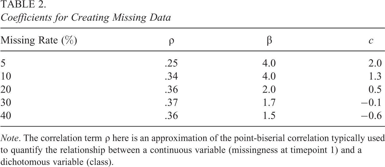
Note. The correlation term
To create MCAR missingness, for each outcome variable (outcome at each timepoint), a randomly drawn value from 0 to 1 from a uniform distribution was compared against a specified threshold that created an overall rate of missing. In this way, the missingness was completely haphazard and adhered to the rules of MCAR missingness. Percentages of 5, 10, 20, 30, and up to 40 were investigated for both missingness conditions.
Data analysis and other common simulation issues
After creating data with different types of missing data, the five different missing data handling approaches, LD, FI, MI, 2M, and FB were utilized to analyze each dataset. These methods were implemented using Mplus Version 8.1 (Muthén & Muthén, 1998–2017) and R (R Development Core Team, 2008). A total of 800 conditions were replicated 100 times. The replication value was chosen based on the minimum number of replications it took for the estimates of the means and variances to converge for the cell with the most suboptimal crossed-conditions (40% missing, LD, with an SS of 100 and very poor separation).
Convergence
To avoid local maxima solutions, the final likelihoods were replicated by varying the number of starting values and setting a maximum number of replicated likelihoods, as per Tueller and Lubke (2010). For the current study, 100 replications with perturbed starting values were conducted and a minimum criteria of 10 optimized likelihoods were used as a sign of convergence to the global maximum. For the Bayesian methods, convergence was assessed using the proportional scale reduction (PSR) factor, where a PSR of 1 with a tolerance of
Label switching
Label switching, a known issue in simulation studies involving finite mixture models (Tueller et al., 2011), was also addressed. For the FB method, within-chain label switching was avoided by constraining the prior for the intercept of one class to be greater than the prior for the intercept of the other class. This prevented the Gibbs sampler from switching midchain. Between-chain label switching was avoided by using a single chain. Label switching between replications for the MLEM method was to be avoided by constraining the class 1 mean intercept to be greater than class 2 mean intercept and class 1 mean slope to be less than class 2 mean slope (Cassiday et al., 2021).
Choice of priors
In certain situations, variances of growth factors are especially susceptible to prior misspecification (Depaoli, 2013; McNeish, 2016). To investigate the kind of priors that should be used for the growth model in the current simulation study, a preliminary simulation was conducted on the full data (without any of the missing data conditions) to see how different priors would affect variance parameter estimation. The simulation involved comparing MLEM and a Bayesian MCMC method using prior specifications for the variance parameters as suggested by McNeish (2016) for LGMs. Priors for the means were not specified and left as diffuse because past studies found these parameters to be invariant across different priors. The same priors tested by McNeish (2016) were also tested for this preliminary study: an improper, noninformative, inverse Wishart distribution prior (Mplus default), a proper, noninformative, inverse Wishart distribution distribution prior, and a data driven prior using estimates from an initial MLEM run. The results from the complete data study showed that the noninformative (inverse Wishart) prior for the variances actually performed well compared to the other priors. Although these findings were inconsistent with suggestions from past studies, the improper, noninformative priors seemed to be the best choice to use for this particular situation for the missing data handling methods that were compared.
Number of imputations
It has been suggested that the number of imputations for MI be set at
Evaluation of Outcomes
Each cell in the simulation was evaluated based on convergence, classification accuracy, relative bias of the parameter estimates, and precision of the SEs. In order to pinpoint any effects of the manipulated conditions on the parameter estimates, a split-plot design factorial analysis of variance (ANOVA) was conducted. In this particular design, the missing data handling method was regarded as a within-subject factor, and all other conditions were considered between-subject factors. All main effects (SS, class separation, missing mechanism, MR, and missing data handling method) and up to three-way interactions were considered on the relative bias and SE bias of the estimates of the means, variances, and class proportion parameters (nine parameters in total: two intercept means, two slope means, intercept and slope variances, intercept and slope covariances, residual variances, and two class proportions). Only factors and interactions that were identified as statistically significant (p value
Classification accuracy
To answer the first research question of interest, classification accuracy was evaluated based on the percentage of correct and incorrect classifications. High classification accuracy meant that a high percentage of individuals classified into the class they belong in the population, and a low percentage of individuals classified into a different class than where they belong in the population. Most likely class memberships for each individual were obtained from the posterior probability after estimation. These class assignments were then compared to the individual’s true class assigned at the time of data generation.
Parameter recovery
To answer the second research question of interest, for each condition, parameter recovery of the fixed effects and respective random effects for the set number of replications were assessed using relative bias. That is
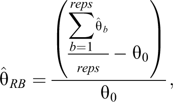
where
To answer the third research question of interest, bias of the SEs of the estimates, or the analogous posterior standard deviations (SDs) of the estimates for the Bayesian method, was evaluated by the ratio between the square root of the mean variance of
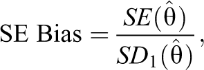
where
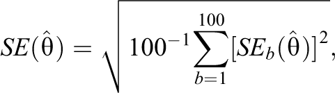
and
Results
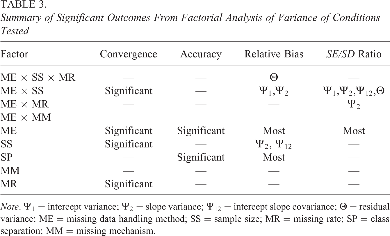
Provided in Table 3 is a summary of the results from each of the factorial ANOVA analyses that were conducted on the outcome measures. A nonempty cell in the table is indication that differences were significant among all the conditions tested. For example, the table shows that the different missing data handling methods (ME) produced differences in the rates of convergence, accuracy, relative bias, and SE/SD ratios. A three-way interaction between method, SS, and MR was also flagged for the relative bias of the residual variances. In addition, a two-way interaction was flagged between method and SS for the convergence rates, relative bias of the intercept variance, and slope variance estimates, as well as the SE/SD ratio of all the variance estimates. This table was used to pinpoint specific conditions for which the outcomes were significantly different. While many differences in the conditions could have been reported, we focus on a few differences in order to focus on answering the research questions of interest. Specific results that are not discussed in this study are available from the first author by request.
Summary of Significant Outcomes From Factorial Analysis of Variance of Conditions Tested
Note.
In addition to the missing data analyses, full-data GMM analyses were conducted in order to establish appropriate comparisons for the different missing data analyses. The full-data analyses involved running a two-class GMM analysis on the data without any missing data, estimated two different ways. The first method of estimation was using the MLEM approach. The second approach was using a Bayesian estimation method using the Mplus default inverse Wishart (IW) prior specification for the variances of the growth factors. In a separate study, these priors produced the least biased estimates and were considered a good baseline for comparison. Results for the full-data analyses are not presented and are made available only by request.
Convergence and Accuracy
The convergence rates were generally lower for the missing data analyses (LD, FI, MI, FB, and 2M) than the rates obtained from the full-data analyses (MLEM and IW), as can be seen in Table 4, which shows the convergence rates for each method across all the SSs tested. The LD method produced the lowest convergence rates, which were as low as 28%. The FI method produced relatively low convergence rates compared to using MI, FB, and 2M, with a convergence rate as low as 39% when the SS was 100. The Bayesian approach produced the highest rates of convergence, even when SSs were as small as 100, never going below 80%. The 2M method also produced relatively high rates of convergence, although not as high as the FB approach, staying between 81% and 89% convergence rates.
Convergence Rates Across Method and Sample Size Using Missing Data Methods

Note. MLEM = maximum likelihood via expectation-maximization; IW = inverse Wishart; LD = listwise deletion; FI = full-information ML via EM; MI = single-stage multiple imputation; FB = fully Bayesian; 2M = two-stage multiple imputation.
Although no significant interaction was detected for differences in the classification accuracy rates, classification accuracy decreased uniformly as separation decreased, as can be seen in Table 5. The FB approach maintained the closest accuracy rates to its full data counterpart. Accuracy rates decreased when the 2M method was used. Using LD, FI, and MI had a very minimal impact on the classification accuracy rates compared to the rates produced when using full data MLEM. Accuracy rates went from 53% when the separation was very poor to 66% when the separation was high. At the very poor classification condition, all the methods produced the same poor results of around 51% to 53% accuracy rates. The classification accuracy rates were also slightly better for the Bayesian method and the imputation methods across all separations, with the largest difference observed between FB and FI when the class separation was moderate. When the separation was high, FI, MI, and 2M produced similar classification accuracy rates, but the FB method was around 6% higher than all other methods. As expected, the missing data conditions dropped the classification accuracy rates across all methods.
Classification Accuracy Rates Across Method and Separation Using Missing Data Methods

Note. MLEM = maximum likelihood via expectation-maximization; IW = inverse Wishart; LD = listwise deletion; FI = full-information ML via EM; MI = single-stage multiple imputation; FB = fully Bayesian; 2M = two-stage multiple imputation.
Parameter Recovery
The discrepancies across methods in the overall absolute relative bias measures can be clearly seen in Figure 1. Overall, the relative bias of the FB and 2M methods was closest to their full-data counterpart (IW) and was all under the 10% acceptable threshold. This is evidence that the FB and 2M methods produced similar estimates as when the data were not missing, regardless of how much data were missing or which missing data mechanism was used. The large discrepancies between the means and medians of the absolute relative bias measures indicate that the overall bias may be isolated to a few parameters that produced extremely biased parameter estimates. The LD, FI, and single stage MI methods produced higher mean absolute relative bias values than MLEM method, although the medians were lower.
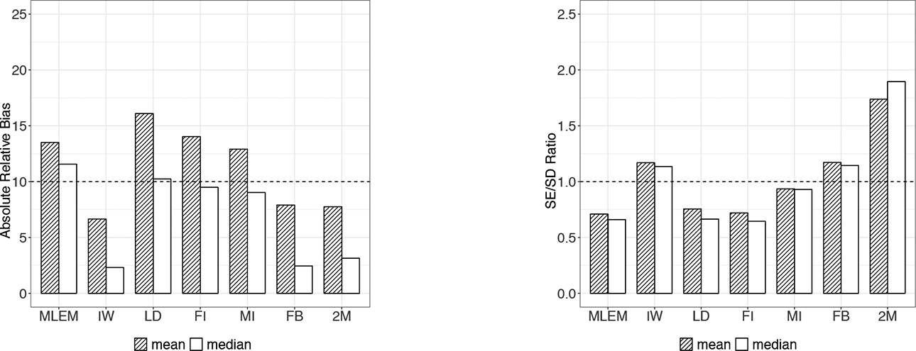
Left: Overall absolute relative bias across methods (ME). Right: Overall SE/SD ratios across methods (ME).
Examining the relative bias of all the estimated parameters for each method (Figure 1), for the Bayesian methods, these spikes in the means were likely due to the large relative bias measures produced by the class 1 and class 2 slope means, the slope variances, and intercept slope covariance measures. This is also seen in Table 6, where the relative bias passed the 10% threshold when missing data were incorporated and analyzed using the FB method in the estimation of the intercept variances (from 8% to 10%) and the intercept slope covariances (from 6% to 19%). For the MLEM-based methods, the large bias measures were attributed to class 1 and class 2 slopes, as well as intercept variances and intercept slope covariances. Table 6 shows how the slope means, intercept variances, slope variances, and intercept slope covariances were generally downward biased for the MLEM-based methods. For some parameters, like the intercept slope covariance parameter, LD and FI exacerbated the bias, increasing the relative bias from −20% to −45% for the LD method and to −26% for the FI method.
Relative Bias for Select Parameters Across Methods
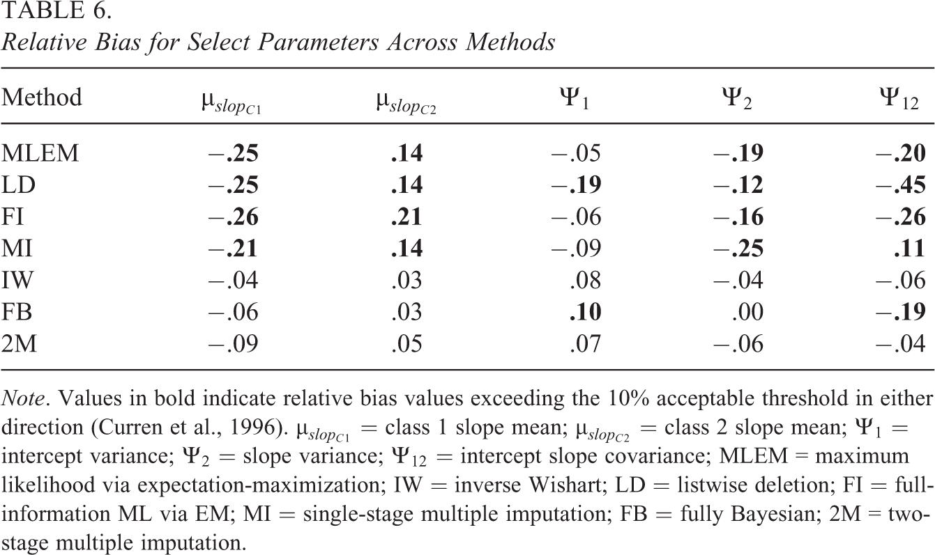
Note. Values in bold indicate relative bias values exceeding the 10% acceptable threshold in either direction (Curren et al., 1996).
Overall, very poor and high separation conditions produced a select number of parameters with large relative bias. Table 7 shows that the largest measures of relative bias occur for the estimates of the slope means, intercept variances, slope variances, and intercept slope covariances. Estimates of the slope means and slope variances were most negatively biased (22% and 21%, respectively) when separation was very poor (MD = 0.5) and improved as class separation increased to high (MD = 2.0), reaching negative relative bias measures of −13% for the slope means and −12% for the slope variances. The reverse occurred for the intercept slope variance estimates, where the bias increased from −21% to −40% when class separation went from MD = 0.5 to MD = 2.0.
Relative Bias for Select Parameters Across Class Separation

Note. Values in bold indicate relative bias values exceeding the 10% acceptable threshold in either direction (Curren et al., 1996).
A closer look at the two-way interaction between SS and method for the intercept variances, slope variances, and residual variances shown in Figure 2 reveals different patterns of relative bias across SSs and methods. For example, larger SSs in general produced relative bias measures close to zero and within the 10% criteria. For MLEM-based methods, the bias increased uniformly downward as SS increased but was magnified when using the LD method followed by the MI method. The LD method produced values below the threshold even at sample sizes of 500. The Bayesian methods performed better at all SSs above 200, where the FB method produced estimates with positive relative bias right above the 10% threshold. At SSs of 100, all methods including the full-data method produced biased estimates of the intercept variance.
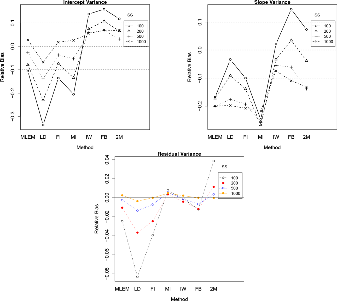
Interaction plots for ME
Estimates of the slope variances produced by the MLEM method were severely underestimated to begin with and with the addition of missing data conditions, methods like MI produced even more underestimated parameters across all SS conditions. The Bayesian approaches were mostly within the boundaries of the acceptable bias range except when the SSs were at 100 or 1000. Estimates were already underestimated for the full-data counterpart, and when missing data conditions were added, the FB and 2M methods exacerbated the negative bias for SSs of 500 and 1000. At SSs of 100 and 200, the relative bias swayed the opposite direction, where the relative bias estimates moved upward.
Finally, the three-way interaction between SS, method, and MR can be easily observed in Figure 3. Although the residual variances were generally not severely biased, the plot for SS 100 shows that the relative bias was extremely underestimated when the MR was 40% and LD was used. In general, the bias observed across methods and MR was as expected: larger missing data rates and smaller SSs produced more biased parameter estimates of the residual variances.
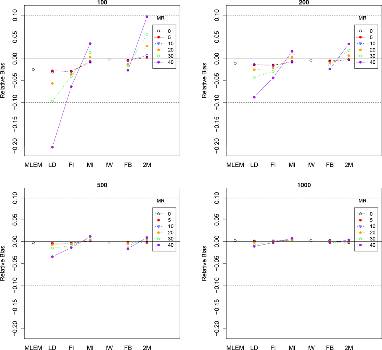
Three-way interaction ME
Discussion
In this study, several different methods for handling missing data in the context of GMMs were examined across realistic analytic conditions. Findings from the simulation study showed both expected and unexpected results. The MI method produced higher rates of convergence, even than the rates produced from the full data ML method. This may have been an artifact of the MI method being a quasi-Bayesian method in that imputations were drawn from a data augmentation process that is FB. This may be supported by the fact that the Bayesian-based methods had the highest rates of convergence (greater than 80% across SSs) and that the MI method produced rates approaching these values.
The accuracy rates across methods when missing data conditions were introduced were mainly indistinguishable for very poor class separation. The FB method, however, produced the highest accuracy rates with poor, moderate, and high class separation conditions, while the other methods produced similar accuracy rates. The lower accuracy rates that were observed for the 2M method were somewhat surprising, given that the parameter estimates were quite comparable to the FB method. In retrospect, this may have been because of how these accuracy rates were collected for the 2M method during the simulation, which was different from how accuracy rates were collected for nonimputation methods. In any case, this issue warrants a deeper investigation into how the accuracy parameters were collected during the simulation.
Overall, MLEM-based methods produced higher relative bias measures than Bayesian and Bayesian-based methods. The discrepancies between the means and medians of the overall absolute relative bias pointed to certain parameters as the main culprits of this bias. For all methods, including methods using the full data, slope means, intercept variances, and intercept slope covariances were always problematic, and the slope variance was also problematic for MLEM-based methods. Specifically, the slope variance and intercept slope covariances were consistently underestimated. These results were consistent with the growth modeling literature, which has pointed to the issue that even with complete data, some ML methods under a growth modeling SEM framework will underestimate factor variances and SEs (Browne & Draper, 2006), even though large SSs should correct for these discrepancies. In this regard, Browne and Draper (2006) and also McNeish and Harring (2017), who conducted a similar study of LGMs with a focus on samples of less than 100, recommend using a restricted version of the ML method to obtain unbiased parameter estimates. The issue has to do with how in an SEM framework, variance parameters are estimated around a fixed effect, which is more difficult to accomplish with smaller SSs. The suggested remedy according to these studies was to use a restricted version of ML estimation method, which uses a separate process to estimate the fixed effects parameters. The bias observed in this study was also partially supported by the results presented in Depaoli (2013), which showed that slope variances and sometimes the intercept and intercept slope variances were consistently underestimated when using the standard MLEM method (the default in Mplus). Bayesian-based methods also seem to have remedied this issue, as was seen by the relatively smaller measures of relative bias for all the variance terms.
The slope means were also consistently under- or overestimated, regardless of whether MLEM or a Bayesian method was used. These results generally corroborated results from Depaoli (2013), which showed biased slope means regardless of the prior that was used (unless the true parameters were used, which is unrealistic).
The SEs were consistently overestimated for 2M method, while in general, the FB method produced SE to SD ratios closest to 1, albeit overestimated SEs observed when SSs were at 100 and 200. The LD, MI, and FI methods, which were grounded on MLEM, produced underestimated SEs. These results were actually consistent with what was observed by McNeish (2016), where the Bayesian MCMC methods using noninformative priors produced overly wide coverage intervals (overestimated SEs), while FI consistently had coverage intervals that were too short (underestimated SEs). The reverse impact that the priors had on the SEs of the intercept means was interesting (SE ratios converged to 1 as SSs increased using noninformative priors, while they deviated upward from 1 as SSs increased using data driven priors). In addition, SEs were severely underestimated for the intercept means when using data driven priors, which may have been an artifact of the priors specified for the variance parameters since priors were not specified for any of the means.
LD and MI methods performed relatively poorly compared to FI, FB, and 2M, which was consistent with Enders (2011), who suggested avoiding MI for mixture models altogether. However, a firm recommendation is impossible to make based on these results because the MI approach used MLEM to analyze the imputed datasets, which as was observed, produced relatively poor results. It is impossible to tell from these results whether the bias occurred because of the missing data imputation process or because of the estimation of the datasets. On the contrary, 2M seemed to be a viable alternative, albeit producing poor estimates of the SEs.
One interesting observation from this study is that the differences when imposing an MCAR as opposed to a CMAR+ missingness mechanism were minimal, and whether the missing data approaches did anything to improve estimation when missingness was the more severe CMAR+ missingness was not very clear from the results. With multiple group models, Enders (2011) and Sterba (2016) suggested that the missingness mechanism was inconsequential to how poorly the MI method would perform. In this regard, it made sense that there was very little difference observed between the estimates from the two missingness mechanisms. However, these results suggest that additional investigations are needed because the MLEM estimates were already producing poor estimates to begin with, making the MI method incomparable to the 2M method.
Based on the findings from the simulation study, the Bayesian inference and 2M methods may serve as viable alternatives to FI and MI in terms of producing less biased parameter estimates for GMMs. However, this comparison warrants further investigation, given that the full-data analysis step of the MI method was conducted using MLEM, which produced relatively more biased estimates compared to the Bayesian method. Although choosing priors can be challenging, the advantages in terms of producing higher convergence rates, higher classification accuracy rates, less biased parameter estimates, and more accurate SEs (for the Bayesian approach) are certainly worth the additional preliminary investigation prior to the analysis. One disadvantage of using the 2M method is that although the tools are available in Mplus, the setup is more involved and requires the researcher to take additional steps outside of Mplus. The steps that were taken to conduct the two-stage imputation method for this study are fully disclosed in the online Appendix.
Even with the use of noninformative, diffuse priors, the FB approach was superior in regard to the evaluation criteria that were considered, especially with the estimation of the SEs. While the 2M method was relatively better than MI method and FI in terms of recovering parameter estimates, the SEs were generally overestimated, which in practical applications would have led to inflated Type II error rates. These recommendations should be taken with caution since many real-life conditions were kept consistent, a rare occurrence in any real data scenario.
Supplemental Material
Supplemental Material, sj-docx-1-jeb-10.3102_10769986221149140 - Handling Missing Data in Growth Mixture Models
Supplemental Material, sj-docx-1-jeb-10.3102_10769986221149140 for Handling Missing Data in Growth Mixture Models by Daniel Y. Lee and Jeffrey R. Harring in Journal of Educational and Behavioral Statistics
Footnotes
Declaration of Conflicting Interests
The author(s) declared no potential conflicts of interest with respect to the research, authorship, and/or publication of this article.
Funding
The author(s) received no financial support for the research, authorship, and/or publication of this article.
Note
References
Supplementary Material
Please find the following supplemental material available below.
For Open Access articles published under a Creative Commons License, all supplemental material carries the same license as the article it is associated with.
For non-Open Access articles published, all supplemental material carries a non-exclusive license, and permission requests for re-use of supplemental material or any part of supplemental material shall be sent directly to the copyright owner as specified in the copyright notice associated with the article.
