
Abstract
Inter-rater reliability (IRR), which is a prerequisite of high-quality ratings and assessments, may be affected by contextual variables, such as the rater’s or ratee’s gender, major, or experience. Identification of such heterogeneity sources in IRR is important for the implementation of policies with the potential to decrease measurement error and to increase IRR by focusing on the most relevant subgroups. In this study, we propose a flexible approach for assessing IRR in cases of heterogeneity due to covariates by directly modeling differences in variance components. We use Bayes factors (BFs) to select the best performing model, and we suggest using Bayesian model averaging as an alternative approach for obtaining IRR and variance component estimates, allowing us to account for model uncertainty. We use inclusion BFs considering the whole model space to provide evidence for or against differences in variance components due to covariates. The proposed method is compared with other Bayesian and frequentist approaches in a simulation study, and we demonstrate its superiority in some situations. Finally, we provide real data examples from grant proposal peer review, demonstrating the usefulness of this method and its flexibility in the generalization of more complex designs.
Keywords
1. Introduction
Inter-rater reliability (IRR) has been used to assess the quality of ratings and assessments in psychology, education, health, hiring, proposal and journal peer review, and with other areas involving multiple raters. From a measurement perspective, individual ratings (such as scores applicants receive from a hiring committee) may be thought of as imprecise estimates of the true underlying quality of a measured subject or object. IRR enumerates the consistency among raters, and it may be described as the correlation between scores of different raters given to the same subject or object of measurement (Webb et al., 2006).
A notable portion of research is focused on the identification of heterogeneity sources in IRR with respect to contextual variables, such as rater or ratee characteristics, with the goal of identifying policies with the potential to generally decrease measurement error and to increase the IRR especially for the lower IRR subgroups. For example, IRR was found to vary for different research areas of grant-proposal peer review (Mutz et al., 2012) and to increase after reviewer training (Sattler et al., 2015). In the context of teacher hiring, IRR was found to be lower for internal than external applicants (Martinková et al., 2018) and lower for novice than experienced applicants (Goldhaber et al., 2021). In the context of teacher assessment, the IRR was found to be higher for the ratings of live versus recorded lectures (Casabianca et al., 2013).
Different estimation techniques were considered in the past to account for heterogeneity in IRR with respect to groups. The most common approach involves stratification of the data and separate estimation of IRR in subgroups with analysis of variance (ANOVA) or mixed-effect models (Sattler et al., 2015). More complex mixed-effect models allowing for heterogeneous variance components were shown to detect group differences in IRR even in those cases where no difference was detected using the stratification approach (Martinková et al., 2018). Another method is based upon generalized-estimation equations (Mutz et al., 2012). Bartoš et al. (2020) compared different methods for IRR estimation under heterogeneity with respect to a single grouping variable in a simulation study, where the data-generating model was known, showing that both frequentist and Bayesian mixed-effect models, as well as general additive models, can provide accurate estimates of group-dependent IRR.
However, further methodological complexities arise in real-life situations, which were not solved by previous studies. The variance components of the ratings may be affected by a combination of contextual factors, such as the rater’s or ratee’s age, gender, major, or internal versus external status, which may be of different types (besides binary also nominal, ordinal, or metric). Furthermore, the model specification—inclusion or exclusion of the different contextual factors—might need to be inferred from the data. Researchers might also be interested in whether a particular contextual factor does or does not affect the variance components, that is, testing a hypothesis whether the effect of a given factor differs from zero. To our best knowledge, there has been no study estimating IRR or reliability with heterogeneous variance mixed-effects models in cases of heterogeneity due to a combination of covariates. None have dealt with model selection, nor is any general approach available.
To fill this existing research gap, we propose a flexible general approach to IRR estimation and hypothesis testing using Bayes factors (BF) in those cases of variance heterogeneity due to covariates and unknown data-generating models. Our work builds upon studies of Bayesian mixed-effects models with heterogeneous variance components (Williams et al., 2020; Williams et al., 2019), which were previously shown to provide a richer understanding of the psychological processes in various contexts, and upon the work of Dablander et al. (2020), who recently introduced a default BF test for the inequality of variances. We also consider model-averaged estimates, which incorporate uncertainty in the model selection process for the final estimate (Depaoli et al., 2020; Hoeting et al., 1999; Raftery, 1996; Raftery et al., 1995).
This article proceeds as follows: We first introduce the IRR in the multilevel modeling framework. We extend it to heterogeneous variance components and introduce Bayesian hypothesis testing and model averaging in Section 2. Second, we describe a simulation study and compare the proposed methodology to alternative approaches in Section 3. Third, we illustrate the methodology on real data sets from ratings of the grant proposals in Section 4. Finally, in Section 5, we conclude with a discussion of the results and of further computational aspects of IRR estimation, including the aspects of generalizations in more complex designs. Sample
2. Methods
2.1. IRR in Multilevel Modeling Framework
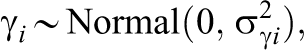
In the simplest case of a multilevel linear model with a one-way ANOVA, rating j of subject i, denoted

where
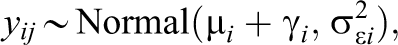
Under the model defined by Equation 1, IRR is defined as the ratio of the true variance due to ratees,
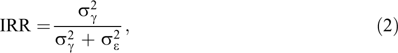
corresponding to the intraclass correlation coefficient denoted as ICC(1,1) (see McGraw & Wong, 1996; Shrout & Fleiss, 1979, for more details and further possibilities).
The variance components in IRR defined by Equation 2 can be estimated using various frequentist and Bayesian approaches to provide an estimate of IRR. The maximum likelihood (ML) estimates are found as parameters maximizing the likelihood function given the data (Searle, 1997). The REstricted (or REsidual) ML (REML) method is an adaptation, in which the marginal likelihood function is maximized with respect to variance components
Finally, the Bayesian estimation (e.g., Gelman & Hill, 2006) starts with specifying prior distributions for all model parameters (the variance components
2.1.1. Incorporating heterogeneous variance components
The multilevel model defined by Equation 1 can be further generalized. The generalization suggested here involves the variance terms, possibly together with the mean, depending on covariates. For

where the mean


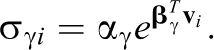
In this equation,
Under a model defined by Equation 3, the
Note that when including covariates
Also note that we generally allow a possibly different set of covariates
2.2. Bayesian Hypothesis Testing and Model Averaging
With Equation 3 denoting the most complex model, a number of submodels can be considered as special cases based on restricting some of the effects in
2.2.1. Bayes factors
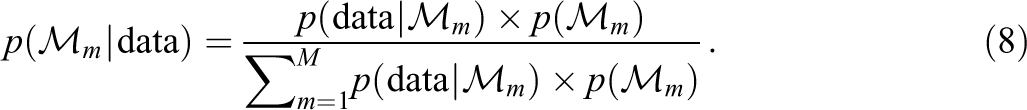
We consider here the Bayesian hypothesis testing framework of Jeffreys (1931), which evaluates the evidence in support of/against any model by the usage of BFs. BFs are computed as a ratio of the marginal likelihoods of the competing models (Etz & Wagenmakers, 2017; Kass & Raftery, 1995; Rouder & Morey, 2019; Wrinch & Jeffreys, 1921)
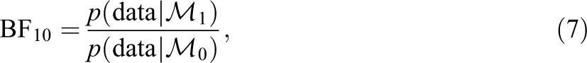
with the marginal likelihood
The BF is a continuous measure of evidence in favor of
2.2.2. Bayesian model averaging
In addition to model selection and using the single best-fitting model for parameter estimation, we should consider Bayesian model averaging (Hoeting et al., 1999; Kass & Raftery, 1995; Leamer, 1978).
Bayesian model averaging accounts for the uncertainty of model selection by weighting the posterior model estimates by posterior model probabilities. First, we need to assign prior model probabilities
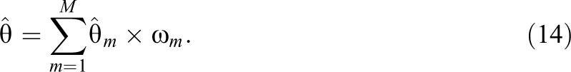
We then combine the posterior parameter estimates

which allows us to acknowledge the uncertainty about the considered models. We follow a common convention in Bayesian model averaging and assign an equal prior model probability to models assuming the absence and presence of the difference between the groups for either the mean, structural, or residual variance, resulting in
Furthermore, Bayesian model averaging allows us to quantify evidence in favor of including a specific parameter across the whole set of specified models with a comparable structure. For example, for a difference between the groups in a residual variance
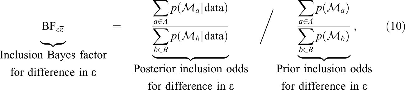
where A represents a set of models for which the groups differ in the
2.2.3. Parametrization and choice of priors
To employ the Bayesian framework consisting of BFs and Bayesian model averaging, we need to complete the models by specifying prior distributions for all the parameters in Equations 4 and 5. Here, we restrict ourselves to consideration of binary covariates, testing for and quantifying the differences between groups (see Section 5 for suggestions on dealing with other types of covariates). We use effect coding (i.e., we assign the values of −0.5 and 0.5 for the two levels), so the prior distribution on the regression coefficients
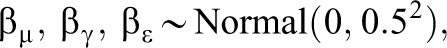
For the simulation study and the real-data example, we use the following priors:

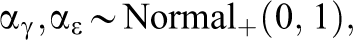
where
where
Our reasoning behind the choice of priors is as follows: Since the intercept parameters are common across all models (i.e., we are not going to test for the presence or absence of the intercept), we can specify weakly informative prior distributions on them (Gelman & Hill, 2006). Here, we use standard normal prior distribution for the grand mean intercept,
In contrast to the common intercepts, the regression parameters
To assess the robustness of our results to the prior distribution specifications, we use two other choices of

Visualization of different options of prior distributions on the regression coefficients. We used the Normal (0,
3. Simulation Study
We perform a simulation study to assess the performance of the outlined methodology. We are specifically interested in an estimation and hypothesis testing in consideration to the differences between groups in any of the modeled parameters (i.e., means, structural standard deviations, and residual standard deviations) and IRR. We keep simulation settings simple, in order to compare the outlined methodology to other model selections and model-averaging techniques, considering that many of the other methods could not deal with more complex data settings.
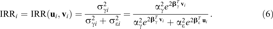
For the simulation, we consider IRR in a group-specific variance components model; in other words, we assume a single binary covariate, the group membership denoted by index

where
Under the model specified by Equation 12, the group-specific
and it takes the two values of
Possible submodels of the model defined by Equation 12 are derived as special cases based upon restricting the group-specific parameters under a combination of conditions:
Altogether, the combination of conditions A, B, and C leads to seven possible submodels denoted as M1 through M7, and one unrestricted model (Equation 12) denoted as M8:


3.1. Data Generation
Data generation was inspired by real data encountered in the context of teacher applicant ratings (Martinková et al., 2018). Specifically, in Equation 12, we used two values for the standardized mean differences between the groups (
Data Generation Scenarios
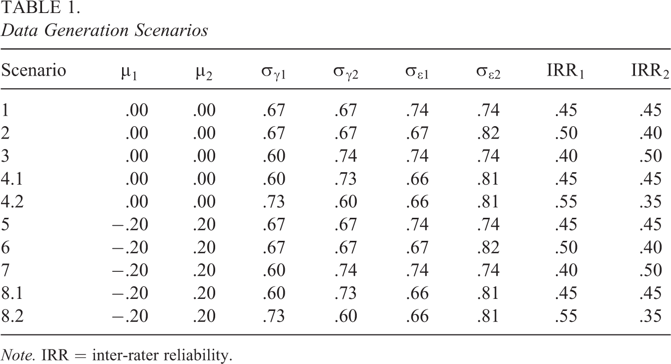
Note. IRR = inter-rater reliability.
Moreover, we manipulated the number of times the ratees were rated (J = 3 or 5) and the number of ratees per group (I = 25, 50, 100, or 200) in each scenario. In total, 10 (scenarios including subscenarios)
3.2. Compared Methods
We compared the Bayesian hypothesis testing and model-averaging methodology outlined in Section 2 to alternative frequentist and Bayesian ways of estimating and testing for the differences in group-specific mixed-effects location scale models defined by Equation 12. Specifically, we used the ML and REML estimation in the frequentist framework for linear mixed models and Markov chain Monte Carlo estimation in the Bayesian framework.
3.2.1. Model selection
To assess the performance of the model selection with BFs specified in Section 2.2.1, we considered four frequentist model selection approaches and two Bayesian approaches.
The frequentist approaches include two stepwise selection procedures (backward and forward) and two model space selection procedures based upon Akaike information criterion (AIC; Akaike, 1974) and the Bayesian information criterion (BIC; Schwarz, 1978). In the forward stepwise selection procedure, we started with the simplest model. We first tested for adding the difference in means (with REML) and then gradually tested expanding the model with differences in structural and/or residual variances (with ML; see the left panel of Figure A1 in Appendix A for diagram). In the backward stepwise selection procedure, we started with the most complex model. We first tested for gradually removing differences in the structural and/or residual variances (with ML) and then tested for removing the difference in means (with REML; see the right panel of Figure A1 in Appendix A for the diagram). In the model selection procedures based upon information criteria, we estimated all the specified models (with ML) and subsequently selected the best-fitting model based on the lowest information criteria (AIC or BIC).
The Bayesian approaches include two model space selection procedures based upon posterior predictive performance—the Watanabe-AIC (WAIC; Watanabe & Opper, 2010) and leave-one-out (LOO) cross-validation (Vehtari et al., 2017). WAIC and LOO approximate the LOO prediction error using the log-likelihood evaluated with posterior parameter distribution (McElreath, 2018). While they are asymptotically equivalent, LOO usually performs better in small samples and under weak prior distributions (Vehtari et al., 2017). In our case, we use the individual ratings
3.2.2. Model averaging
To assess the performance of the parameter estimation with Bayesian model averaging, we used two frequentist and two alternative Bayesian approaches.
The frequentist methods combine the estimates
The two frequentist approaches are based on information criteria (AIC and BIC), and specify the weight
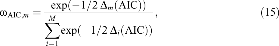
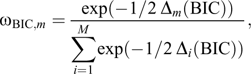
with


where
As an alternative Bayesian approach, the pseudo-Bayesian model averaging (BMA), similarly to the frequentist model averaging, uses information criteria to compute the model weights in Equation 15 (Geisser & Eddy, 1979; Gelfand, 1996). In contrast to Bayesian model averaging, it does not require specification of prior model probabilities, since the weights are based entirely on the LOO information criteria.
The last alternative approach, the Bayesian stacking of predictive distributions (Yao et al., 2018), is based upon stacking, which combines models in order to minimize LOO mean square error (MSE; Breiman, 1996; LeBlanc & Tibshirani, 1996; Wolpert, 1992). The stacking of posterior distribution is then based upon the LOO predictive distribution computed with LOO. Similar to pseudo-BMA, Bayesian stacking does not require specification of prior model probabilities; however, it oftentimes does not allow inference about the true data structure and is unable to provide compelling evidence in favor of simple models (Gronau & Wagenmakers, 2019a, 2019b).
3.3. Evaluation of the Simulation Results
We first evaluate the proportion of selecting the correct model based upon BFs and we compare it with other approaches. We evaluate the proportion of correct model selection averaged across all conditions and separately for each of the data generating model and sample size.
Next, we compare our approach with other approaches in the precision of estimates of model parameters and of IRR. As a measure of precision, we evaluate the root mean square error (RMSE). As a (relative) measure of bias, we also evaluate the bias2/MSE ratio. This is again evaluated when averaged across all conditions, as well as for all the individual model generating designs.
Finally, we evaluate the calibration of our prior distributions and of inclusion BFs with the so-called Bayes factor design analysis (see, e.g., Schönbrodt & Wagenmakers, 2018; Stefan et al., 2019, for more details). Our goal for this simulation was (1) to verify that the inclusion BFs found evidence in favor of the difference in parameters in those conditions, where the parameters differed and evidence in favor of no difference in conditions where the parameters do not differ, (2) to evaluate the proportion of misleading evidence, that is, how often would the inclusion BFs find strong evidence in favor of a difference in scenarios with no difference present, and finally (3) to verify that the evidence is increasing with an increasing sample size.
3.4. Implementation
The simulation was carried out in
3.5. Simulation Results
3.5.1. Model selection
We first take a look at the averaged results across all conditions. The probability of selecting the correct model is summarized in Table 2. BFs, AIC, WAIC, and LOO are able to identify the correct model with precision around 26% of the time in the smallest group sizes (N = 25); however, while BFs and AIC steadily improve with increasing sample sizes (up to 70% and 65% respectively), WAIC and LOO start lagging behind. Furthermore, the stepwise forward and backward selection procedures start catching up with the BFs with increasing sample sizes (69%).
Proportion (and Standard Error of Proportion) of the Correctly Selected Models (Averaged across Conditions, Number of Ratings per Rated Subject j = 3)
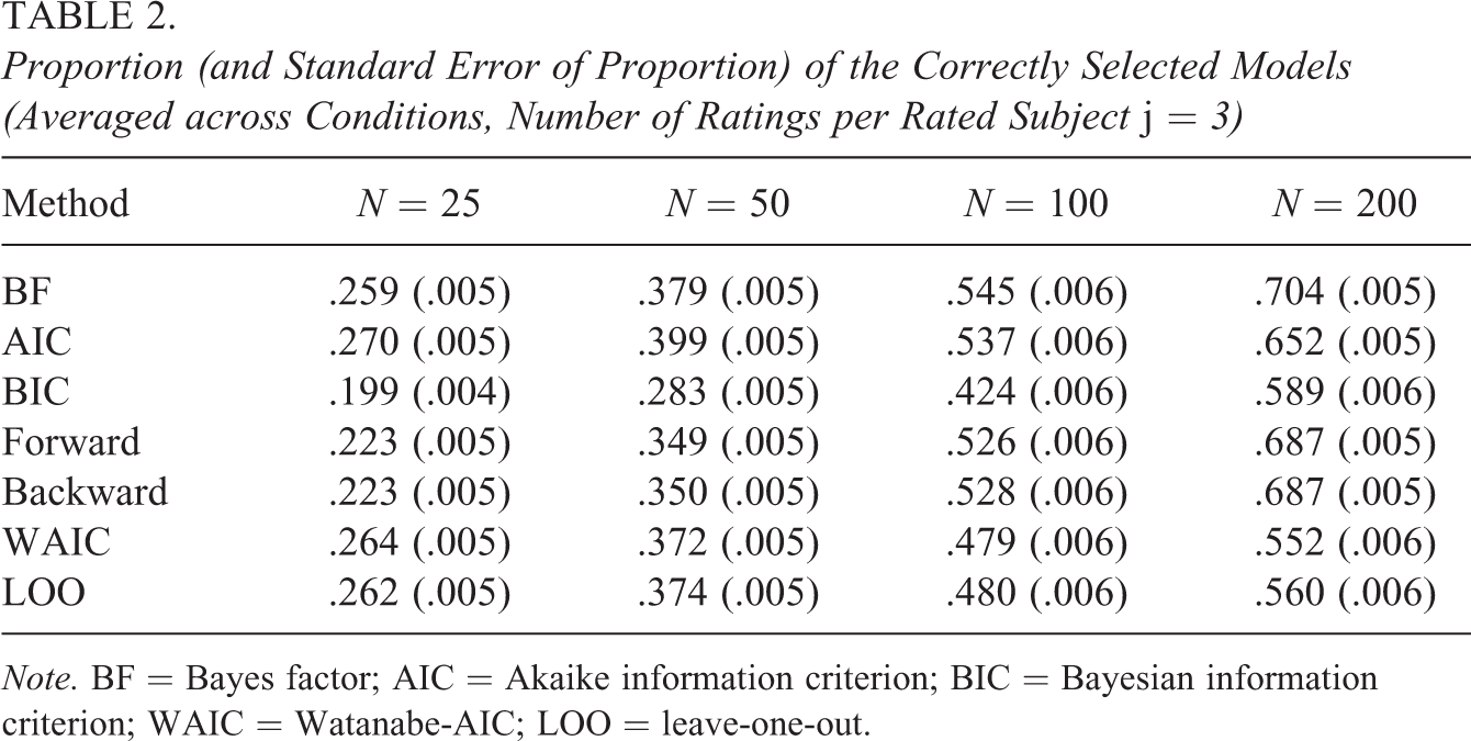
Note. BF = Bayes factor; AIC = Akaike information criterion; BIC = Bayesian information criterion; WAIC = Watanabe-AIC; LOO = leave-one-out.
Figure 2 displays model selection performance for individual data-generating designs. The first column shows the proportion of correctly selected models, the second column shows the proportion of selecting a more complex incorrect model (i.e., a model containing all true parameter differences plus some additional incorrect differences), and the last column shows the proportion of other incorrect models (models missing at least one parameter difference). We see a well-known behavior of BIC being biased toward the simpler model, resulting in “better” performance under data-generating scenario 1, and a bias of WAIC and LOO toward more complex models, resulting in a lower proportion of correct model selection and increased selection of incorrect more complex models in the simpler data-generating designs. The same trends are visible in the case of
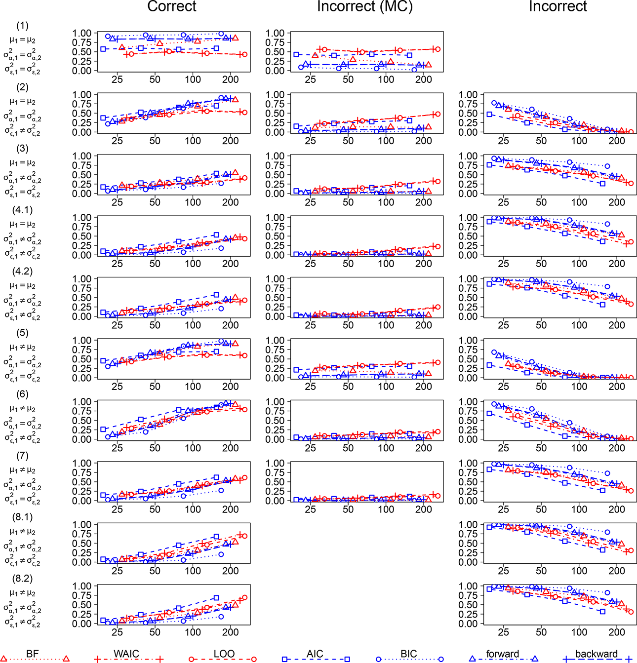
Proportion of correct, incorrect—more complex (MC, containing all true parameter differences plus some additional incorrect differences), and incorrect (missing at least one parameter difference) model selection. Red: Bayesian. Blue: Frequentist model selection techniques. BF: Model selection with Bayes factor proposed here.
3.5.2. Parameter estimation
The RMSE of the residual SD estimates, averaged across all conditions, is summarized in Table 3. We can see that with small samples (e.g., N = 25), the model averaging leads to more precise estimates of residual variance than the estimates based upon the selected best-performing model. For example, Bayesian parameter estimation in the models selected with BFs resulted in RMSE of 0.075, while the Bayesian model averaging resulted in RMSE of 0.069. With a growing sample size, the uncertainty in model selection disappears, and the RMSE of the two approaches converges to the same value. The same trend can be seen for the IRR estimates in Table 4; however, the benefits of model averaging are less pronounced than in the case of residual variances.
RMSE (and Standard Error of RMSE) of the Residual SD Estimates (Averaged across Conditions, Number of Ratings per Rated Subject j = 3)
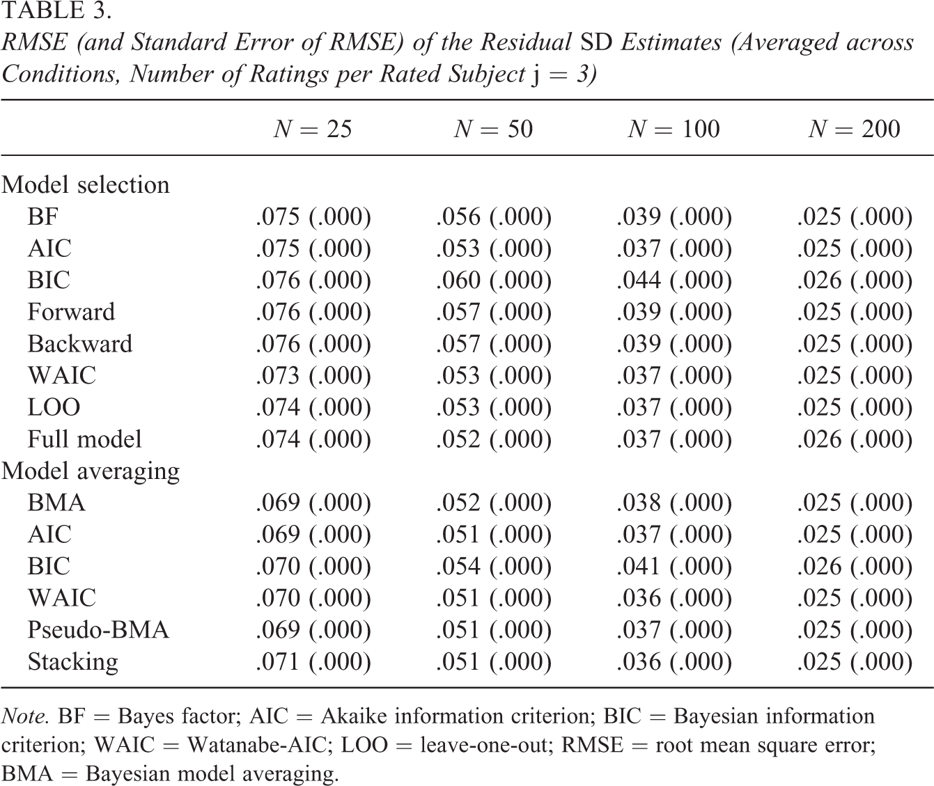
Note. BF = Bayes factor; AIC = Akaike information criterion; BIC = Bayesian information criterion; WAIC = Watanabe-AIC; LOO = leave-one-out; RMSE = root mean square error; BMA = Bayesian model averaging.
RMSE (and Standard Error of RMSE) of the IRR Estimates (Averaged across Conditions, Number of Ratings per Rated Subject j = 3)
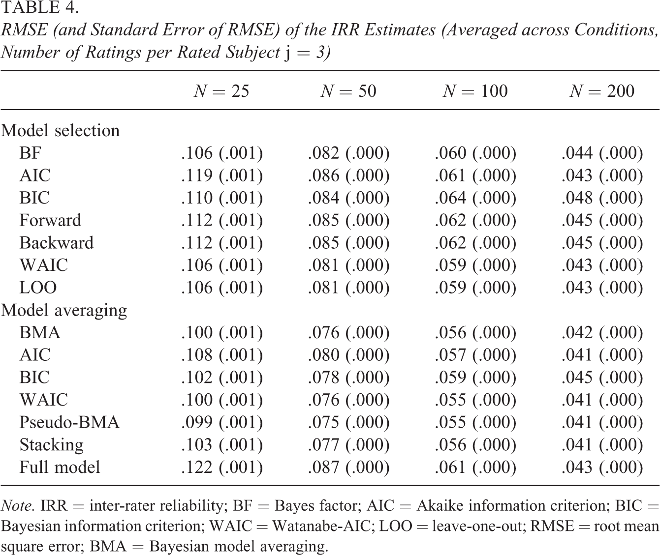
Note. IRR = inter-rater reliability; BF = Bayes factor; AIC = Akaike information criterion; BIC = Bayesian information criterion; WAIC = Watanabe-AIC; LOO = leave-one-out; RMSE = root mean square error; BMA = Bayesian model averaging.
Analogous tables with the RMSE of the mean estimates and structural variances, which are not the main focus of IRR and our study, are available in the electronic Supplementary Material, as well as the corresponding results for
3.5.3. Inclusion BF calibration
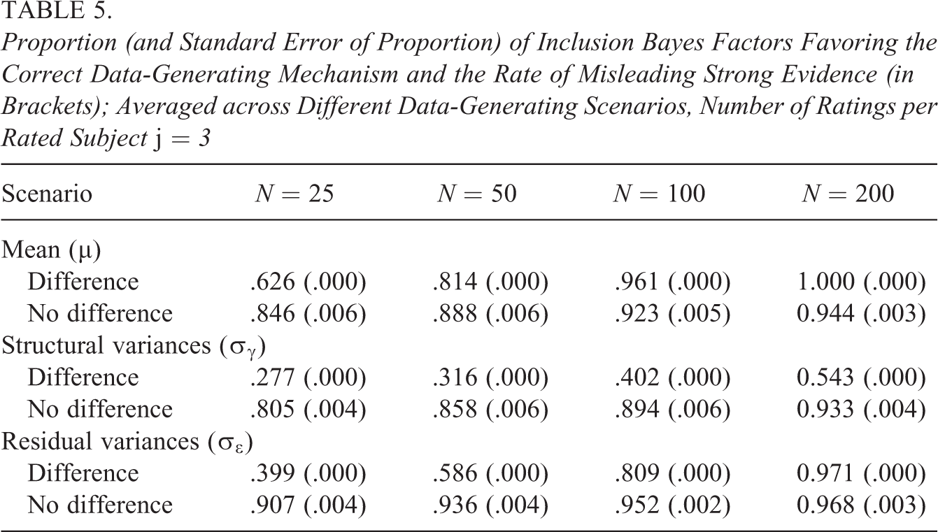
Finally, we turn our attention to performance of the inclusion BFs in providing evidence for differences in the mean, the structural, and the residual variance between the two groups. Table 5 summarizes the proportion of inclusion BFs correctly favoring the true data generating model for each parameter in both types of scenarios (with difference vs. without difference in a given parameter), averaged across data-generating scenarios of a given type, and the rate of misleading strong evidence (
Proportion (and Standard Error of Proportion) of Inclusion Bayes Factors Favoring the Correct Data-Generating Mechanism and the Rate of Misleading Strong Evidence (in Brackets); Averaged across Different Data-Generating Scenarios, Number of Ratings per Rated Subject j = 3
A more detailed behavior of the inclusion BFs is depicted in Figure 3, visualizing the distribution of (
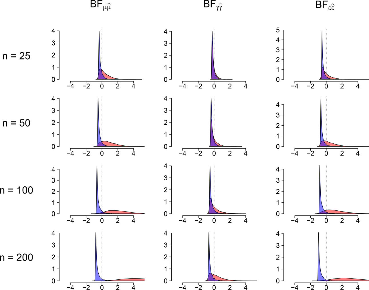
Visualization of
We can see that inclusion BFs for differences in means
4. Real Data Examples
We demonstrate the estimation of IRR with two datasets of grant proposal peer-review analyzed by Erosheva et al. (2021) and available in the
Unlike in the simulation presented in Section 3, with the real data, the true generating model is unknown. However, the practical examples provide an illustration regarding the application of the proposed method; for the first two examples incorporating a single covariate, we can also compare the results with those provided by other methods presented in the simulation study.
In our analysis, we assume that the selection panels may take the applicant’s gender and career stage into consideration when interpreting the ratings, that is, we allow covariates to explain the fixed part
4.1. AIBS Grant Proposal Review Data With Single Covariate
The first example involves peer-review ratings of the American Institutes of Biological Sciences (AIBS), analyzed by Erosheva et al. (2021). In the AIBS data set, each grant proposal was rated three times on the number of criteria as well as on the overall merit score considered here as the dependent variable. The gender (n female = 25 and n male = 47) of the principal investigator was used as a covariate/grouping variable.
The BF, as well as other model selection methods (both Bayesian and frequentist), indicated the simplest model (M1) was the most suitable for the data (Table 6). However, there was a relatively large uncertainty about the selected model, as can be seen from Table 7, which summarizes the weights for the individual models. The simulation study suggested that with this small sample size, all methods have a low probability of selecting the correct model, and it is hard to judge which of the models is true. The simulation also demonstrated that the model selection based upon BIC more often prefers simpler models, which can also be observed in our practical example, where the model weight based upon BIC is much higher (0.78) for model M1 than the weights for this model based upon other criteria.
AIBS Peer-Review Example: IRR Estimates for Female (G1) and Male (G2) Principal Investigators

Note. BF = Bayes factor; AIC = Akaike information criterion; BIC = Bayesian information criterion; WAIC = Watanabe-AIC; LOO = leave-one-out; BMA = Bayesian model averaging; IRR = inter-rater reliability; AIBS = American Institutes of Biological Sciences; ICC = intraclass correlation coefficient.
AIBS Peer-Review Example: Model Weights
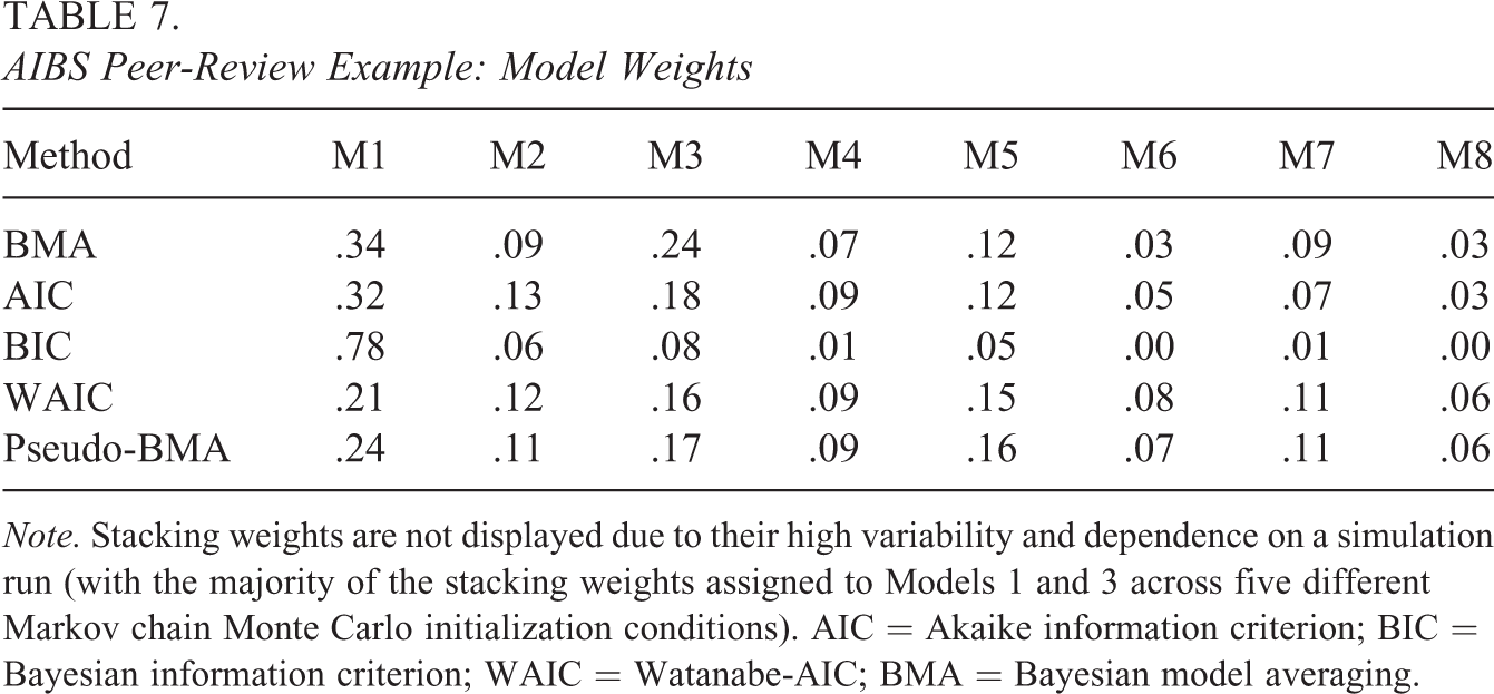
Note. Stacking weights are not displayed due to their high variability and dependence on a simulation run (with the majority of the stacking weights assigned to Models 1 and 3 across five different Markov chain Monte Carlo initialization conditions). AIC = Akaike information criterion; BIC = Bayesian information criterion; WAIC = Watanabe-AIC; BMA = Bayesian model averaging.
Quantifying the evidence across all models with inclusion BFs resulted only in weak evidence in support of the absence of difference in the means,
4.2. NIH Grant Proposal Review Data With Single Covariate
For the second example, we used the data of peer-review ratings of the National Institutes of Health (NIH), analyzed by Erosheva et al. (2020) and further discussed in Erosheva et al. (2021). We used the preliminary Investigator criterion scores and the gender (n female = 574 and n male = 1310) of the principal investigator as a covariate.
All model selection methods selected models which assumed a difference in residual variances: BFs and BIC suggested Model M2, the model selection based upon LOO, WAIC, forward, and backward selection also suggested a difference in means (Model M6), while the method based upon AIC selected the most complicated model also suggesting a difference in structural variances. According to Models M2 and M6, the single-rater IRR for grant proposals by male PIs is 0.36 (0.33 – 0.39), whereas for grant proposals by female PIs it is 0.33 (0.29/0.30 – 0.36) with a difference in IRR of 0.04 (0.01/0.02 – 0.06). However, according to model M8, the difference of IRRs for male and female PIs is insignificant −0.01 and with a wider CI of (−0.07 – 0.05) also covering zero (see the top panel of Table 8).
NIH Peer-Review IRR Estimates Investigator Scale of the Complete Data Set of “Male” (G1) and “Female” (G2) Principal Investigators
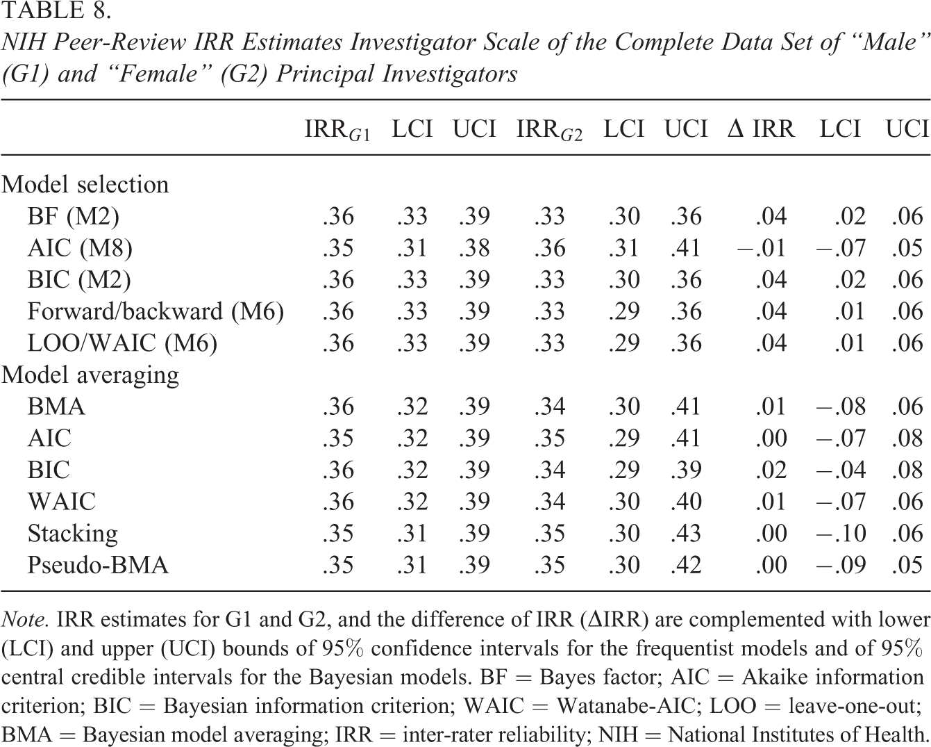
Note. IRR estimates for G1 and G2, and the difference of IRR (
Despite a much larger sample size than in the previous example, there is still considerable uncertainty about the selected model (see Table 9). We again use model averaging to account for the model uncertainty, which results in wider confidence intervals. Most of the approaches find differences in IRR between the two groups insignificant, with a confidence interval of
Model-Averaging Weights for NIH Peer-Review IRR Estimates Investigator Scale of the Complete Data Set of “Male” (G1) and “Female” (G2) Principal Investigators
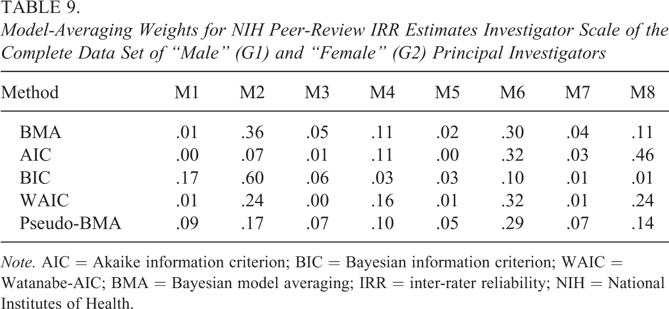
Note. AIC = Akaike information criterion; BIC = Bayesian information criterion; WAIC = Watanabe-AIC; BMA = Bayesian model averaging; IRR = inter-rater reliability; NIH = National Institutes of Health.
Quantifying the evidence across all models with inclusion BFs resulted only in weak evidence in support of the absence of difference in the means,
4.3. NIH Grant Proposal Review Data With More Covariates
We finally considered a more complex situation of IRR being dependent upon two covariates: gender and binarized career stage. In this case, the model given by Equation 12 has 64 submodels. Model selection using BFs identified that the data were best predicted by a model in which the means, structural variances, and residual variances differed by career stage, with the posterior model probability of 0.23. Table 10 shows 10 models, which were best at predicting the data, accumulating a total of 95% of the posterior model probabilities. We can see that despite the large sample size and the considerable uncertainty about the best model, most of the best-performing models consider the career stage to be an important predictor for all parameters. However, gender does not seem to play a central role and is slightly more often not even considered.
Model Structure for the 10 Best-Performing Models in the NIH Data Set When Considering Both the Gender and Career Stage as Predictors
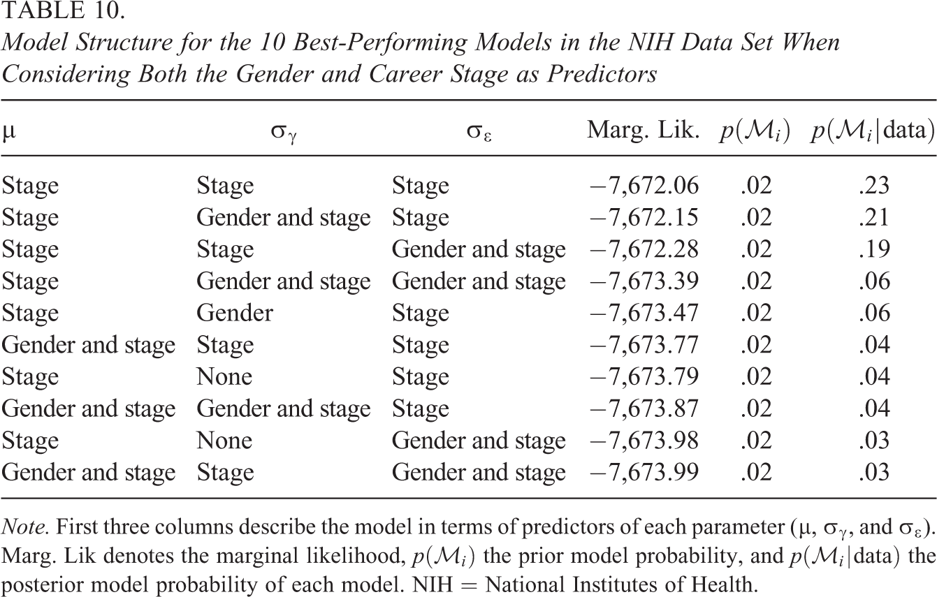
Note. First three columns describe the model in terms of predictors of each parameter (
An overall picture is provided using Bayesian model averaging, which combines estimates and evidence across all models. We find weak evidence against difference in residual variance between the two gender groups,
While the residual variance is a parameter of central importance for the assessment of measurement error and IRR, we may also derive from the results conclusions regarding structural variance, the mean, and regarding between-group differences in these parameters. We find weak evidence against difference in structural variance between the two gender groups,
Higher residual variance in the nonexperienced group is accompanied by only slightly higher structural variance, and it leads to a somewhat lower IRR (see Table 11). Note that when only the models with no covariate effect on the mean are considered, the structural variance in the nonexperienced group is higher, leading to higher IRR in this group (see Table A4 in Appendix C).
Estimated Model-Averaged Marginal Means and 95% CI for Each of the Parameters
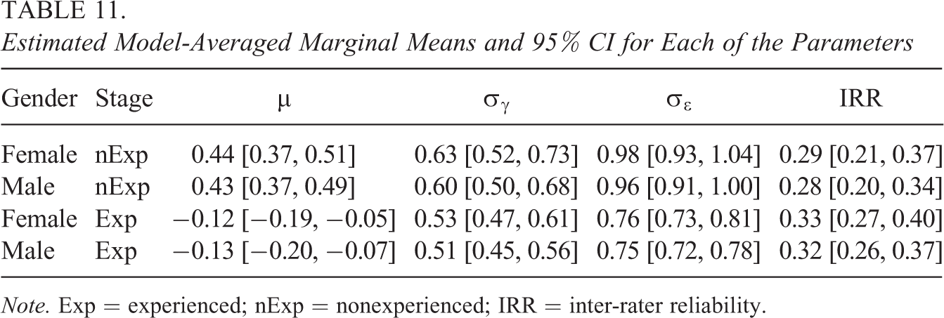
Note. Exp = experienced; nExp = nonexperienced; IRR = inter-rater reliability.
We further conducted a sensitivity analysis to assess how our conclusions would change if we specified different prior distributions, that is, tested different hypotheses. We used the two remaining prior distributions depicted in Figure 1; (1) a more concentrated prior distribution around no effect with the standard deviation
We will only discuss here the residual variances (see Appendix B for more details). Between the two gender groups, we found strong evidence for the absence of larger differences in the residual variances and no evidence supporting the presence or the absence of small differences. For the groups segregated by career stage, we found very strong evidence for presence of the effect, regardless of the specification of the alternative hypothesis. In other words, the data were more consistent with no or small differences in residual variances between the two gender groups and there was clear evidence in favor of differences in residual variances between the two career stage groups.
5. Discussion
In this work, we have presented a new flexible approach for assessing the IRR in cases, where variance components, depending upon covariates, are assumed to differ. We used mixed effect models with heterogeneous variances and employed the Bayesian framework with BFs and Bayesian model averaging. In a simulation study, we compared the methodology to other frequentist and Bayesian approaches and shown comparable or superior performance to those of the other methods. More importantly, flexibility in the proposed methodology allows researchers to straightforwardly extend the presented models to cases with more covariates, whereas BFs can be used to select a single model, researchers can further account uncertainty in the model structure with Bayesian model averaging when drawing inferences about either the presence or absence of the effect via inclusion.
The suggested methodology—Bayesian hypothesis testing and model averaging—is, of course, not the only option researchers can pursue. Authors with different philosophical views would advocate for different approaches, such as estimation only or inference based upon confidence intervals (e.g., Cumming, 2014; Gelman & Hill, 2006). We prefer the Bayesian hypothesis testing since we believe that BFs (and likelihood ratio tests) are the only coherent method of testing for the presence versus absence of the effect. The problem with hypothesis testing based upon posterior credible intervals (or p values) is the assumption of either the presence (for credible intervals) or absence (for p values) of the effect at the onset of the analysis. In other words, it is impossible to provide evidence for/against an assumption that is already taken for granted (e.g., Jeffreys, 1939).
The advantages of Bayesian hypothesis testing and model averaging, however, come at an additional cost: the specification of prior distributions. Prior distributions are especially important upon the parameters of interest, where they define the hypotheses about the presence versus the absence of an effect. Different prior distributions equal to different hypotheses—different questions—being asked. Subsequently, different questions might lead to different answers (e.g., a one-sided vs. two-sided test). Nonetheless, as shown by the sensitivity analysis in Appendix B, similar prior distributions correspond to similar questions, which subsequently result in similar answers. To define a prior distribution, researchers must be able to define the degree of effects they are interested in (see, e.g., Johnson et al., 2010; Mikkola et al., 2021; O’Hagan et al., 2006, for detailed information about prior distribution elicitation).
The proposed method was further demonstrated when assessing IRR in a grant proposal peer-review with respect to the applicant’s gender and career stage. The results suggested that the IRR is not likely dependent upon the gender of the principal investigator, while it may be lower with a lower career stage. When demonstrated in this specific example of grant peer review, it is worth noting the importance and the wide range of possible applications using the proposed method. Our methods may be used to identify gaps in the IRR for various rating situations (applicant hiring or promotion, classroom observation of teachers, journal peer-review, etc.) and with respect to the different types of rater and ratee characteristics (dichotomous such as internal/external status, factors such as social status or marital status, and continuous such as age).
We also discussed how hypotheses regarding specific variance components may be addressed with the inclusion BFs. This is especially important because IRR is influenced by range restriction (Erosheva et al., 2021), meaning that for a fixed residual variance, different values of IRR are obtained depending upon the structural variance. For this reason, the difference between residual variances may be of greater interest than the difference in the IRR itself. This aspect was also demonstrated with the NIH example by comparing the case of when the grand mean was allowed to vary with covariates to the case of no covariate adjustment: In the latter case, the structural variance for the nonexperienced group was higher, leading to a somewhat higher IRR than in the experienced group, while when the ratings accounted for the stage, the structural variance was somewhat lower for the nonexperienced group, leading to a somewhat lower IRR. Unlike IRR which provided contradictory conclusions, the inclusion BFs provided more coherent information and in both cases unanimously concluded there is a significant difference in the residual variance and more error in the ratings from applicants in the nonexperienced group.
Several limitations of the current study and possible directions for future research are worth mentioning: First, a simulation study will always cover only a finite and rather limited number of parameter setups, and our simulation study involved only one binary covariate. Nevertheless, the current simulation study was already extensive in terms of the number of methods compared and the simulation time needed. Besides the computation time, some aspects of the frequentist approaches would need to be solved. As an example, the parametrization is not straightforward in the
Secondly, we considered binary covariates only. However, our approach could be easily extended to other types of covariates. For example, in the case of factors with multiple groups, one has to decide whether an ANOVA-like test for at least one difference between the factor levels should be specified with orthonormal contrasts asserting that the prior marginal levels are identical, making the levels interchangeable (Rouder et al., 2012), or, whether a multiple treatments versus control-like test should be specified with dummy coding, asserting that the control condition corresponds to the grand mean and the coefficients for each treatment condition to differences/standard deviation ratios. Similarly, priors on continuous covariates simply correspond to the unit change in the covariate, with the grand mean/variance corresponding to the covariate value of 0, while the centering or rescaling of the covariate prior to the analysis might simplify the prior specification.
Thirdly, we considered only the simplest model with the ratee being the single structural source of error, while all other possible sources of error (such as rater, occasion, etc.) were encompassed in the residual error. This model is appropriate and widely used when most of the raters rate only a single ratee. In real-life applications, the hierarchy may be more sophisticated (respondents nested within institutions, which themselves are nested within towns or countries), and there may be more sources of error such as raters, the so-called facets in the context of the generalizability theory (Brennan, 2001). Different generalizability and dependability coefficients may then be defined in such cases, and the IRR of interest may need to be defined by more complex ratios with different interpretations. However, the cases of heterogeneity would then be treated analogously, and the Bayesian approach suggested here would be easily applied to more complex situations.
Regardless of the limitations, the study offers a flexible method for assessing the heterogeneity in IRR with respect to rater and ratee characteristics. This may help identifying the subgroups with lower IRR and improving the IRR of these groups and in general. This in turn may be of great importance to those designing the ratings and to policymakers whose interest is to improve assessment systems and the selection processes.
Footnotes
Appendix
Acknowledgments
The authors appreciate the computing and storage facilities of the Institute of Computer Science (Czech Republic RVO 67985807) and access to computing and storage facilities owned by parties and projects contributing to the National Grid Infrastructure MetaCentrum provided under the program “Projects of Large Research, Development, and Innovations Infrastructures” (CESNET LM2015042). They are thankful to Martin Otava, Jon Kern, and anonymous reviewers for their helpful comments and suggestions on earlier versions of this article.
Declaration of Conflicting Interests
The author(s) declared no potential conflicts of interest with respect to the research, authorship, and/or publication of this article.
Funding
The author(s) disclosed receipt of the following financial support for the research and/or authorship of this article: The study was funded by the Czech Science Foundation grant number 21-03658S.