Localized trend model for stock market sectoral indexes movement profiling

Abstract

Previous studies have found that one of the main challenges in the area of time-series analysis is the lack of ability to reveal the hidden profiles of observed dynamic systems. Therefore, this study applies an adaptive clustering method named the Localized Trend Model to extract and group dynamic recurring trends from trajectories of multiple time-series data to expose their underlying profiles of movement. Consequently, in this research localized dynamic profiles of movement between sectoral indexes from the Indonesia stock exchange market in the year of 2016 are extracted, analyzed and utilized to predict their future values as a case study. Results of conducted experiments confirmed that the employed method is capable to perform movement profiling for the Indonesia sectoral indexes and be of help to better understand their imperative basic behavior. Furthermore, the study has also verified the proposition that the ability to better understand profiles of movement in a collection of time-series data would benefit to increase prediction accuracy.

Keywords

time-series analysis dynamic systems adaptive clustering localized trend model multiple time-series profiles of relationship

1. Introduction

The task of time-series modeling has been widely viewed as a set of activities to construct a general model, whereby a single global model is induced from all available past experiences or in this case the historical data (Widiputra, 2014; Pears, Widiputra, & Kasabov, 2013; Widiputra, Pears, & Kasabov, 2011a). In relation to this, the inductive reasoning, e.g. a regression formula, a neural network (Wang, Zeng, & Chen, 2015; Kourentzes, Barrow, & Crone, 2014; Islam, Yao, Nirjon, Islam, & Murase, 2008), a Support Vector Machine known as the SVM (Chen & Lee, 2015; Langkvist, Karlsson, & Loutfi, 2010; Kasabov & Pang, 2003), etc., are some common realization approaches to the construction of such global model. Additionally, since the global models are built using all historical data then it is assumed that such representations are capable to describe the underlying behavior of observed dynamic systems and furthermore predict their future states.

Nevertheless, it is widely known that in a dynamic systems with high state of uncertainty, i.e. financial market, having a single general model would not be sufficient to explain the fundamental behavior of observed system comprehensively. Moreover, previous studies have also found that when being employed to predict future values, the forecasted trajectories produced by a global model often fail to trace localized turbulences that happen at specific time points (Pears et al., 2013). The explanation behind this actuality is the fact that a global model tends to ignore localized deviations resulting in the production of a smoother trajectories (Widiputra et al., 2011a).

As a matter of fact, localized disturbances should be taken into consideration when one is aiming to build a model that is expected to reveal the inclusive nature of a dynamic system. This proposition is made based on the reality that localized disturbances would be of imposing consequence to capture certain states under which a collection of time-series behave differently in comparison to the mean. Reasonably, a discontinuity in the general curve model is required to be able to accurately confine such phenomenon. Yet, this would then go against the fundamental design philosophy that acts as the basis of the construction of global models as illustrated in Figure 1.

Fig.1

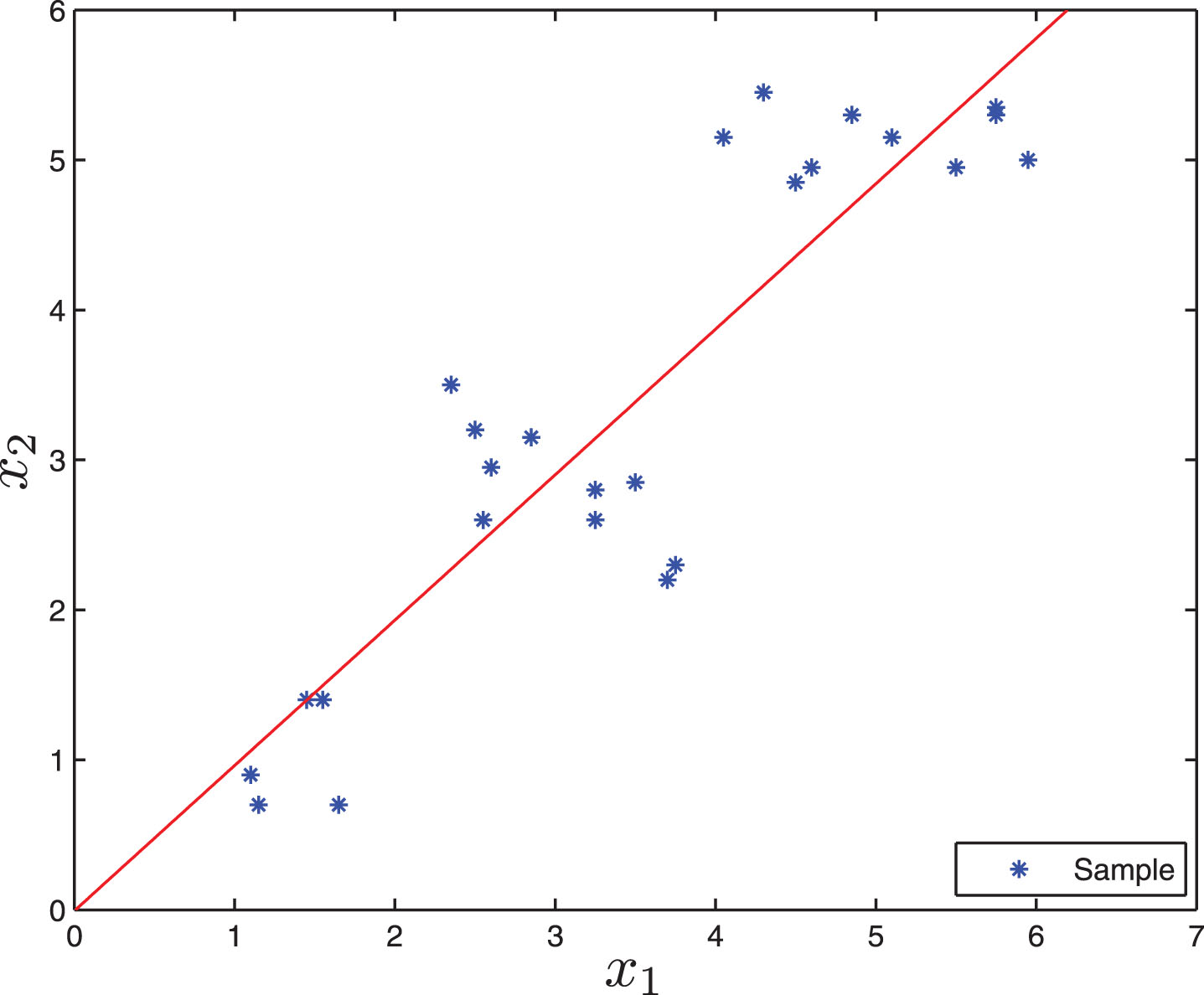
Illustration of global modeling to create localized linear regression model from complete problem set in a 2-D space (Widiputra, 2014).

Thus, it is then of interest to be able to reveal and model profiles of movement from a collection of time-series data originating from particular domain, i.e. financial field. Such profiles can be identified by capturing similar deviations from a global trajectory that take place repeatedly over time, in other words recurring deviations from the usual trajectories that are similar in shape and magnitude. Accordingly, these localized profiles of movement can only be portrayed accurately by local models that are built by learning from data that characterizes the phenomenon under consideration and are unbound from any contamination by data outside the essential phenomenon (Pears et al., 2013).

In relation to the idea that a more detail and accurate fundamental behavior of a dynamic system can be represented by constructing a number of localized models, an adaptive clustering technique for multiple time-series profiles analysis are employed in this study, aiming to: (1) create sub-models that capture recurring behavior as profiles of movement in different time localities from multiple time-series to allow a more comprehensive understanding of the nature of dynamic system under observation; and (2) incorporate such extracted profiles for better prediction of such dynamic system.

In a view of that, this study proposed the use of an adaptive clustering method on a set of multiple time-series data coming from the financial domain, i.e. the Indonesia stock exchange market. In this case, the main objective of the study is to be able to reveal and represent profiles of movement between sectoral indexes in the Indonesia stock exchange market. It is expected that the extracted profiles of movement would benefit to further understand the underlying behavior of financial market in Indonesia particularly and other impulsive dynamic systems in general. The study also seek to proof that more comprehensive understanding about localized profiles of movement would assist to increase general accuracy in predicting the future values of observed dynamic systems.

The next section of the manuscript discuss further the general concept and detail process of utilized adaptive clustering method, followed by the explanation about the interpretation of extracted profiles of movement and how they can be employed for multiple time-series prediction. Experimental results and analysis using the Indonesia stock exchange market sectoral indexes data are then outlined in which its’ profiles of movement are explained and put into test for prediction. Finally, some conclusions are drawn and future works for further exploration are outlined in the final section.

2. Multiple time-series profiling through local modeling

2.1. Concept of localized model

The key idea that act as the core engine for the construction of local models is the split up of the complete problem set into a number of smaller sub-problems according to their position in the problem space to further create localized representations (Widiputra et al., 2011a; Kasabov, 2007; Yamada, Yamashita, Ishii, & Iwata, 2006). These localized representations of the complete problem space are commonly built by grouping together data that has analogous behavior. For example, when the values of a collection of variables are swiftly increasing extensively and then the condition are progressing consistently over a period of time, a natural cluster containing the time points that define this heightened motion can be developed to represent a new conduct of the observed system.

Consequently, as various new types of phenomena are emerging, new localized models or clusters should be defined on their behalf. Specific models can then be developed for each of these clusters, i.e. simple local linear regressions, that will yield better explanation about the nature of the observed dynamic system in that particular local problem spaces covered by the models in comparison to the one represented by a global model, i.e. a model that is constructed over the complete problem space as illustrated in Figure 2.

Fig.2

Illustration of local modeling to create localized linear regression models from clusters of sample data set in a 2-D space (Widiputra, Pears, & Kasabov, 2012).

In the construction process of localized model, individual models are created to evaluate the output function for only a subset of the problem space, e.g. a set of rules over a number of clusters or a set of local regressions. Having a set of local models accordingly offers the possibility of having more comprehensive understanding about the nature of observed dynamic system when being compared to the utilization of a single general model produced by any global modeling technique. The illustration of the localized model concept is depicted in Figure 2.

The existence of multiple localized models would benefit to greater flexibility as when being employed to forecast future values, predictions can then be made either on the basis of a single model or, if needed, at a global level by combining some number of predictions made by the individual local models (Widiputra et al., 2011a; Cevikalp & Polikar, 2008; Kasabov, 2007). Furthermore, the local models are expected to enable the capturing of emerging new behavior in the data and relate them to similar manners from the past. This is different to a global model that is built by considering all past activities, leading to the dilution of recent movements’ effect in the observed data set (Fernandez, Kerre, & Jimenez, 2016; Kasabov, 2007). In this study, the collection of behaviors over local problem spaces of a time-series collection is considered as the time-series profiles of movement.

However, having the practice of clusters creation or clustering as the key process in this approach means that the quality of the clusters is an important foundation for this type of model. The data clustering constraints often need to be adjusted, according to the sub-model’s requirements or the nature of the system that is going to be modeled. Many methods, such as the linear regression need the number of input vectors to be significantly greater than the number of variables and, therefore, the clusters must be large enough to support this type of sub-model. For this reason, the construction of localized models may require more training data than a single global model to confirm that each sub-model is trained with adequate number of samples from the problem space (Aghabozorgi, Shirkhorshidi, & Wah, 2015; Bakoben, Bellotti, & Adams, 2015; Pears et al., 2013).

2.2. The knowledge repository construction

The main objective of the developed local model in this study is to be able to construct a repository of profiles of movement from a collection of time-series data. This repository can be considered as the knowledge repository of observed dynamic system, since it would help to understand comprehensively it’s underlying movement behavior. As described by Widiputra, Pears and Kasabov (2011a), Figure 3 illustrates the general idea of how this repository containing profiles of movement and recurring trends is built and being updated as new manners of movement are emerging when recent data become available.

Fig.3

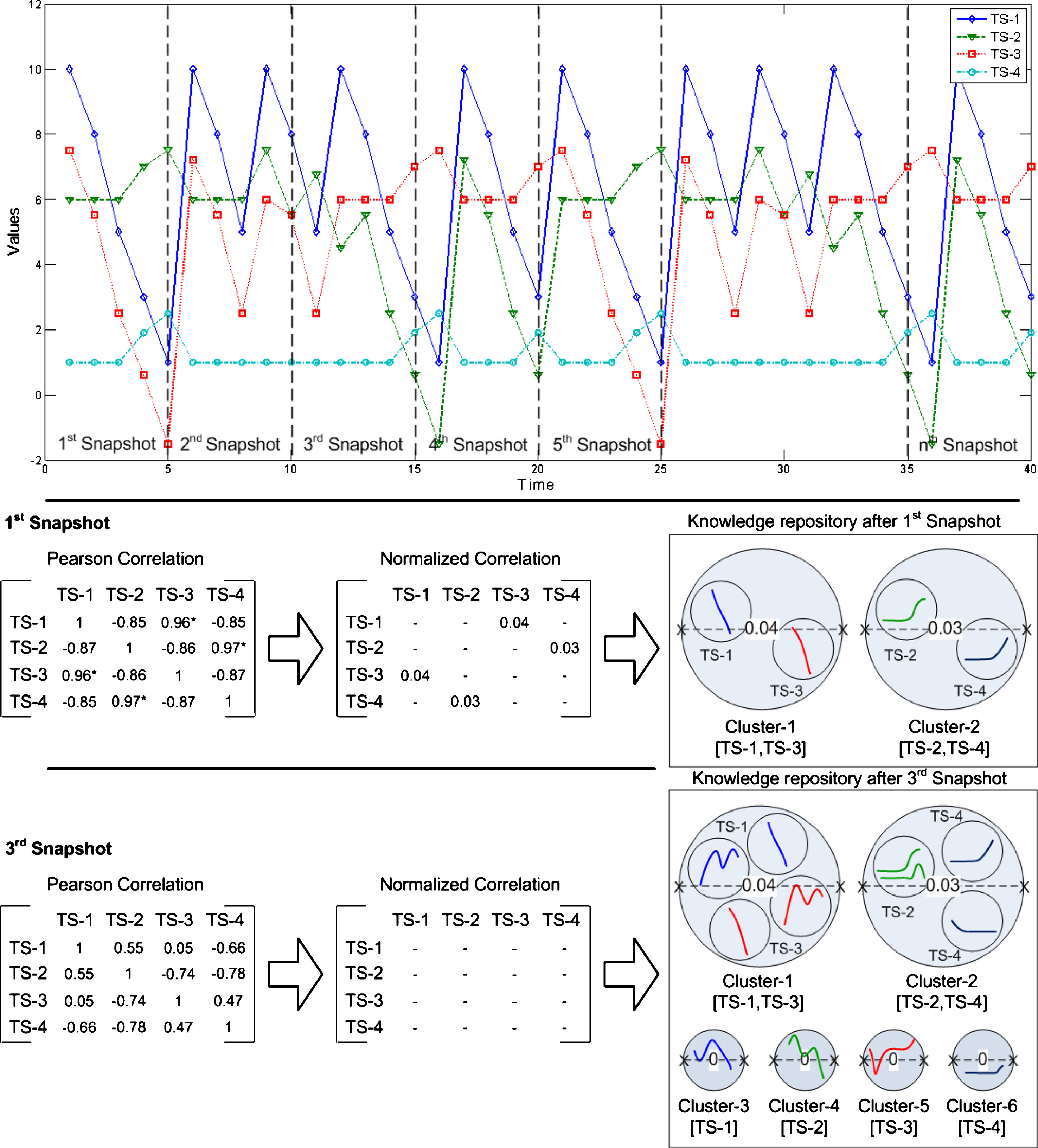
Creation of knowledge repository that represent profiles of movement and their related recurring trends (Widiputra, Pears & Kasabov, 2011a).

The process as portrayed in Figure 3 shows that using data from the first chunk or snapshot, the algorithm extracts two profiles of movement by creating two new clusters. The first cluster represents a profile in which series #1 and series #3 are significantly correlated and moving together, whilst the second cluster is a profile of movement whereby series #2 and series #4 possess comparable shapes of trajectory. Afterward, trends of movement of each series that belongs to a particular profile is then extracted and stored within the profile.

Subsequent to the extraction of trend of movement from each series in the first profile denoted by Cluster-1[TS-1,TS-3], the following process is to create and store the two other trends that belong to Cluster-1[TS-1,TS-3], denoted by TS-1 and TS-3. Here TS-1 and TS-3 represent trends of movement of series #1 and #3 when they are correlated. The same process is then applied to the second profile of series #2 and series #4 denoted by Cluster-2[TS-2,TS-4].

As the second data chunk becomes available, equal procedures to extract are repeated. Since the second data chuck preserves identical profiles of movement, i.e. TS-1 is moving with TS-3 and TS-2 is progressing with TS-4, no new cluster are to be created or stored in the knowledge repository. Yet, new trends of movement from each series are extracted, since the algorithm recognizes that the second data chunk holds a different type of behavior in comparison to the existing ones. Next, the algorithm updates the information about trends of movement of each series in all existing profiles. New clusters of trends are then created and stored in Cluster-1[TS-1,TS-3] and also in Cluster-2[TS-2,TS-4] to represent the emerging new behavior withheld by the second data chunk.

For Cluster-1[TS-1,TS-3], two new models representing current trends are created to characterize a new profile of movement for the collection of series #1 and #3 that diverges from the one which existed in the first data chunk, whereas for Cluster-2[TS-2,TS-4] only a single new instance is created. This is due to the condition whereby the trend of movement for series #2 in the second data chunk is considerably similar to the existing model and therefore it joins the related cluster on its own merits.

Then, as the third data chunk is processed, the algorithm realizes that within this locality of time the four series are uncorrelated and trajecting independently. Thus, new profiles of movement, represented by four new clusters, i.e. Cluster-3[TS-1]; Cluster-4[TS-2]; Cluster-5[TS-3]; and Cluster-6[TS-4], are created for every single series. Each of these new clusters are denoting specific trends of movement detected on the third time locality of the complete series. These procedures continue until there is no more data chunks to be processed or until new data becomes available.

The knowledge repository construction process from a collection of time-series data can be considered as a spatio-temporal modeling process, whereas various shapes of movement (spatio or space) are extracted continuously over time (temporal) as argued by Widiputra, Pears and Kasabov (2011a). In addition, the repository can also be of help to explain how profiles of movement in a system are changing dynamically in different time localities, leading to the retention of different profiles of movement.

3. Adaptive clustering method for movement profiling

As it has been discussed previously, to cover subsets of the problem space that the global model cannot solve with sufficient accuracy, the local modeling approach is required to be put into place. Based on the nature of the model construction, the localized model is actually a specific type of the inductive reasoning process. A system can therefore be represented by a collection of localized models developed from a given data set or observations. However, when being applied to solve new problem, only one model or a subset of the relevant models will significantly contribute to the calculation of the final solution.

This section discusses in detail the exploited methodology for the construction of local models that represent profiles of movement from a collection of time-series data named the Localized Trend Model, hence forward denoted by LTM (Widiputra, Pears, & Kasabov, 2012). The movement profiling procedures in the utilized methodology are consisting of two key phases, i.e. (1) the continuous extraction of profiles of movement of a time-series collection over time, and (2) the clustering of recurring trends when a particular profile of movement emerges.

The principal objective of the methodology is to construct a repository of profiles of movement that further can be utilized as a knowledge-base containing key resource to understand the underlying behavior of the observed dynamic system. To realize such aim, a 2-level local modeling process is utilized within the employed methodology (Widiputra, Pears, & Kasabov, 2011b). The first stage deals with the extraction of profiles of movement between series based on their correlation states to reveal the existence of relationships between pairs of time-series that influence each other.

The second stage of the methodology is to recognize and cluster recurring trends that take place in observed time-series collection when a particular profile of movement is emerging. In this case, the methodology employs a non-parametric regression analysis in combination with the Evolving Clustering Method, known as the ECM (Song & Kasabov, 2001; Kasabov & Song, 2002) to enable the adaptive characteristic in the utilized method.

Alogorithm 1 Extracting profiles of movement from time-series collection

Input:X, where X₁, X₂, . . . , X_n are observed time-series

Output: profiles of movement between series

1: calculate the normalized correlation coefficient [Equation 1] of X

2: for each time-series X₁, X₂, . . . , X_ndo

3: //pre-condition: X_i,X_j do not belong to any cluster

4: if (X_i,X_jare correlated) AND (X_i, X_j do not belong to any cluster) then

5: allocate X_i,X_j together in a new cluster

6: end if

7: pre-condition: X_i belongs to a cluster; X_j does not belong to any cluster

8: IF (X_i,X_jare correlated) AND (X_i belongs to a cluster)then

9: IF (X_jis correlated with all X_i cluster member) then

10: allocate X_j to cluster of X_i

11: else if (X_i,X_j correlation > max(correlation) of X_i with its cluster member) AND (X_jis not correlated with any of X_i cluster member)then

remove X_i from its cluster; allocate X_i,X_j together in a new cluster

13: end if

14: end if

15://pre-condition: X_i and X_j belong to different cluster

16: IF (X_i,X_jare correlated) AND (X_i, X_j belong to different cluster)then

17: IF (X_iis correlated with all X_j cluster member) AND (X_jis correlated with all X_i cluster member)

then

18: merge cluster of X_i,X_jtogether

19: else if (X_i,X_j correlation > max(correlation) of X_j with its cluster member) AND (X_jis correlated with all X_i cluster member)then

20: remove X_j from its cluster; allocate X_j to cluster of X_i

21: else if (X_i,X_j correlation > max(correlation) of both X_i,X_j with their cluster member) AND (X_iis not correlated with one of X_j cluster member) AND (X_jis not correlated to any of X_i cluster member)

then

22: remove X_i,X_j from their cluster; allocate X_i,X_j together in a new cluster

23: end if

24: end if

25: end for

return clusters of profiles of movement

3.1. Continuous movement profiling algorithm

Common activities in the area of time-series clustering have focused more on the task of sample clustering rather than variable clustering (Rodrigues, Gama, & Pedroso, 2008). However, one of the key tasks in the methodology employed in this study to extract profiles of movement from a collection of time-series data is to group together series that are highly correlated and have similar shapes of movement and not samples. This imperative objective stands on the fundamental consideration that multiple local models representing clusters of similar profiles of movement would provide a better basis to comprehensively understand the nature of observed dynamic system than a single global model.

In addition, it is also expected that by having a collection of local models representing the profiles of movement would benefit in making better prediction for the series under examination. An example would be predicting the movement of 6 sectoral indexes in a particular stock exchange market, i.e. Financial, Manufacturing, Property, Automotive, Agriculture, and Mining. If one realizes that currently the Financial and Property sector indexes are progressing together collectively, Manufacture, Automotive and Mining are jointly trajecting, whilst the Agriculture sector index market is moving independently, then it would be relevant to use only information of sectoral indexes from the past which possesses the same profiles of relationships to predict their future rather than to use the entire data set.

Algorithm 1 as it was introduced by Widiputra, Pears, and Kasabov (2012), which was inspired by the work of Ben-Dor, Shamir and Yakhini (1999), outlines the scheme for clustering together similar time-series, in terms of their profile of movement. The first important step of the algorithm is the computation of cross-correlation coefficients between the observed time-series using Pearson’s correlation analysis to recognize significant profiles of relationships between multiple time-series. The Rooted Normalized One-Minus Correlation (RNOMC) coefficients is calculated next to assess the degree of dissimilarity between a pair of time series (a, b) when the most significant correlations between time-series are identified (Rodrigues et al., 2008). The normalized correlation is given by:

$RNOMC (a, b) = \sqrt{\frac{1 - corr (a, b)}{2}}$ (1)

The coefficient would fall between the range of 0 to 1, in which 0 denotes the highest state of similarity between two series and 1 signifies the contrary. Accordingly, when two or more series are grouped together into the same cluster, then diameter represents the highest dissimilarity between two series that are belong to the identical cluster as shown in Figure 4. This concept is the underlying reason to the use of RNOMC in place of the actual correlation as it represents the degree of dissimilarity between a pair of time-series. Such implementation is based on a work by Rodrigues, Gama, and Pedroso (2008) when performing a hierarchical clustering of time-series data streams.

Fig.4

The Pearson’s correlation coefficient matrix is calculated from a given multiple time-series data (TS-1,TS-2,TS-3,TS-4), and then converted to normalised correlation, Equation 1 before the profiles are finally extracted. Figure is extracted from (Widiputra, Pears, & Kasabov, 2011a).

The last stage of the algorithm is to extract profiles of relationship from the normalized correlation matrix. These profiles of relationship should then be interpreted as the profiles of movement since they would show the existence of co-movement between series from the observed dynamic system. In view of that, the methodology used in this step is outlined in lines 3 to 24 of Algorithm 1 while the movement profiling process is illustrated in Figure 1. Basically, the essential concept behind this algorithm is to group multiple series with comparable fashion of movement whilst ensuring that all series that belong to the same cluster are correlated and hold significant level of similarity.

The procedure to cluster trends of movement from each profile follows after all profiles of movement have been extracted from the analyzed time-series collection. Additionally, elements of this procedure is explained in the upcoming section. As the time-complexity of Algorithm 1 is O (n²), where n is the number of series in the analyzed data set, in order to avoid expensive repeating computation, the utilized method stores and dynamically updates extracted profiles of movement only when deviations are recognized instead of redoing the complete set of calculation for every new set of data.

3.2. The clustering process of recurring trends

Having a collection of profiles of movement opens the possibility of the utilized method to reveal certain series that are giving significant effect on the behavior of other series. Nevertheless, this form of knowledge by itself does not offer any predictive power to estimate the future values of observed series on the dynamic system under evaluation.

Consequently, information about different shapes of movement across a group of correlated series needs to be acquired and continuously updated in order to predict future values of a time-series collection simultaneously. Therefore, extraction of emerging trends from all series belonging to a particular profile of movement and it’s utilization to construct multiple local models are imperative to be of help in predicting future drifts.

Generally speaking, to represent trends of movement from different localities of time, the utilized methodology requires a pre-determined form or function, i.e. r^th degree polynomial function, to be provided. However, as trends of movements are changing dynamically in different time localities, the use of a fixed single pre-determined function, e.g. a 3^rd degree polynomial function, to model every trend of movement is considered to be inadequate. Instead, higher degree polynomial functions might be required to better model these more complex trends of movement (Freund, Wilson, & Sa, 2006).

Hence, to overcome such limitations the adopted movement profiling method makes use of a different regression analysis technique that does not require a predetermined form or function to be presented in modeling the trends of movement, i.e. the non-parametric regression analysis. The nature of non-parametric regression analysis which does not require a predetermined function that relates the response to the predictors and does not assume that the observed data set is drawn from a Gaussian data distribution serves as the core motivation of such selection.

In this study, the kernel regression technique is use to realize the non-parametric regression analysis in the movement profiling process. Kernel regression technique is a non-parametric method in statistics used to find a non-linear relation between a pair of random vectors X = (X₁, X₂, . . . , X_n) and Y = (Y₁, Y₂, . . . , Y_n), where n is the number of input/output variables. The goal of kernel regression is to obtain and use appropriate weight vector w, in finding a regression function f (x, w), such that the function is a best-fit match to the data set (X, Y). Here, x is the extended smaller value of the original data X at a certain small step dx calculated using a specific kernel function.

For instance, if a Gaussian membership function is chosen as the kernel function; then x is calculated at domain j where $j = 1, 2, . . ., (\frac{n}{dx} + 1)$ , in a specific small step dx i.e. dx = 0.1, from the original data X = (X₁, X₂, . . . , X_n) by the following equation: $x_{j} = K (x_{j}, X_{i}) = exp (- \frac{(x_{j} - X_{i})^{2}}{2 α^{2}}),$ (2) where x_j = dx × (j - 1), α is a pre-defined bandwidth and i = 1, 2, . . . , n.

To estimate Y_j at domain x_j, Nadaraya and Watson proposed one of the more commonly used kernel regression formula, known as the Nadaraya-Watson kernel weighted average defined as follows (Shapiai, Ibrahim, Khalid, Jau, & Pavlovich, 2010; Nadaraya, 1964; Watson, 1964): ${\hat{Y}}_{j} = f_{j} (x_{j}, w) = \frac{\sum_{i = 1}^{n} w_{i} K (x_{j}, X_{i})}{\sum_{i = 1}^{n} K (x_{j}, X_{i})} .$ (3)

The kernel weights w = (w₁, w₂, . . . , w_n) in Equation 3, can then be estimated using a common parameter estimator method, i.e. OLS or WLS, such that the following objective functions is minimized: $SSR = \sum_{i = 1}^{n} (Y_{i} - {\hat{Y}}_{j}), \forall {\hat{Y}}_{j} where x_{j} = X_{i} .$ (4)

When the LTM is utilized for movement profiling, kernel regression with the Nadaraya-Watson kernel weighted average is used to estimate the regression function that is a best-fit match to the movement of a series in a definitive time locality. Consequently, kernel weight vector w is next considered as a feature vector that represents a trend of movement.

3.3. Recurring trends clustering algorithm

The algorithm to maintain and update recognized trends in each extracted profiles of movement as proposed by Widiputra, Pears, and Kasabov (2012) is outlined in the listed procedures below. This algorithm is the realization of the second phase of the movement profiling procedures as it has been previously explained that the methodology are consisting of two basic phases, which are: (1) extraction of profiles of movement of a time-series collection over time, and (2) clustering of recurring trends for each identified profiles of movement.

In the procedure of movement profiling for a collection of time-series data, in which trend of movement is represented by a kernel weight vector the following indexes are used:

number of data chunks or snapshots: i = 1, 2, . . .;

number of clusters: l = 1, 2, . . . , m;

number of input and output variables: k = 1, 2, . . . , n.

Step 1: perform the autocorrelation analysis on the collection of time-series data from which trends of movement will be extracted and clustered. Number of lags, as an outcome of the autocorrelation analysis where lag > 0, with highest correlation coefficient, is then taken as the size of data chunk or snapshot window denoted as n. The process will then progress by performing a bootstrap sampling process through all data chunks or snapshots;

Step 2: create the first cluster C₁ by simply taking w₁, which is the trend of movement of the first data chunk or snapshot $X^{(1)} = (X_{1}^{(1)}, X_{2}^{(1)}, . . ., X_{n}^{(1)})$ , from the input stream as the first cluster centre c₁ and set the cluster radius R₁ to 0. In this methodology, the i-th trend of movement represented by the kernel weight vector w_i = (w_i1, w_i2, . . . , w_in) is calculated using the Nadaraya-Watson kernel weighted average formula defined as follows: ${\hat{X}}_{j}^{(i)} = f_{j} (x_{j}^{(i)}, w_{i}) = \frac{\sum_{k = 1}^{n} w_{ik} x_{jk}}{\sum_{k = 1}^{n} x_{jk}} .$ (5) Here $x_{j}^{(i)} = (x_{j 1}^{i}, . . ., x_{jk}^{i})$ is the extended smaller value of the original data X⁽ⁱ⁾ at domain j and certain small step dx where $j = 1, 2, . . ., (\frac{n}{dx} + 1)$ . The extended smaller value x_j = (x_j1, . . . , x_jk) is then calculated using the Gaussian MF equation as follows: $x_{jk} = K (x_{j}, k) = exp (- \frac{(x_{j} - k)^{2}}{2 α^{2}}),$ (6) where x_j = dx × (j - 1), k = 1, 2, . . . , n and α is a pre-defined kernel bandwidth. The kernel weight w_i is estimated using OLS such that the following objective functions is minimized: $SSR = \sum_{k = 1}^{n} (X_{k}^{(i)} - {\hat{X}}_{j}^{(i)}), \forall {\hat{X}}_{j}^{(i)} where x_{j} = k .$ (7) To gain knowledge about upcoming trends of movement when a particular trend emerges in a locality of time, the algorithm also models the next trajectory of a data chunk or snapshot by: ${\hat{X}}_{j}^{(i) (u)} = f_{j} (x_{j}^{(u)}, w_{i}^{(u)}) = \frac{\sum_{k = 1}^{n + 1} w_{ik}^{(u)} K (x_{j}^{(u)}, k)}{\sum_{k = 1}^{n + 1} K (x_{j}^{(u)}, k)},$ (8) where $x_{j}^{(u)} = dx \times (j^{(u)} - 1); j^{(u)} = 1, 2, . . ., (\frac{n + 1}{dx} + 1); k = 1, 2, \dots, n + 1$ and the kernel weights $w_{i}^{(u)} = (w_{i 1}^{(u)}, w_{i 2}^{(u)}, . . ., w_{i (n + 1)}^{(u)})$ .

Step 3: if there are no more data chunks or snapshots, the algorithm terminates; else the next data chunk or snapshot, X⁽ⁱ⁾, is processed. The trend of movement from X⁽ⁱ⁾ is then extracted as in Step 2, and distances between current trend and all m existing cluster centres are calculated by $D_{i, l} = 1 - CorrelationCoefficient (w_{i}, c_{l}),$ (9) where l = 1, 2, . . . , m. If, for an existing cluster C_l, D_i,l ≤ R_l, then the current trend joins cluster C_l and the step is repeated; else continue to next step;

Step 4: find a cluster C_a (with centre c_a and cluster radius R_a) from all m existing cluster centres (existing profiles of movement) by calculating the values of S_i,a given by $S_{i, a} = D_{i, a} + R_{a} = min (S_{i, l}),$ (10) where S_i,l = D_i,l + R_l and l = 1, 2, . . . , m.

Step 5: if S_i,a > 2 × Dthr, where Dthr is a threshold that determines the maximum size of a cluster radius, then current trend of X⁽ⁱ⁾, w_i, does not belong to any existing clusters or profiles in this case. A new cluster representing new profile is then created in the same way as described in Step 2, and the algorithm returns to Step 3;

Step 6: if S_i,a ≤ 2 × Dthr, current trend w_i joins cluster C_a. Cluster C_a is updated by moving its centre, c_a, and increasing the value of its radius, R_a. The updated radius $R_{a}^{new}$ is set to S_i,a/2 and the new centre $c_{a}^{new}$ is now the mean value of all trends of movement that belong to cluster C_a. Distance from the new centre $c_{a}^{new}$ to current trend w_i, is equal to $R_{a}^{new}$ . The algorithm then returns to Step 3.

3.4. Profiles of movement repository for time-series prediction

Once the construction of profiles of movement and their related recurring trends repository is finished, another two further steps are required to be executed before the repository can be used for the prediction of observed time-series collection future values. The first step is to extract profiles of movement that exist in the currently observed time locality. Thereafter, matches are to be found from previously stored profiles from the past. Secondly, forecasts are then calculated based on a weighting scheme that allocates more magnitude to pairs of series that withheld similar profile of movement and also retain comparable trends. The weight w_i,j for given pair i, j of a series is determined by the distance of similarity between them.

The prediction process is illustrated in Figure 5, whilst detail procedures for the simultaneous prediction of time-series collection based on the constructed profiles of movement repository, as introduced by Widiputra, Pears and Kasabov (2012), are given as follows:

Step 1: after the profiles of movement repository KR has been constructed based on the observed time-series collection and as the latest observations $x_{t} = (x_{t}^{(1)}, x_{t}^{(2)}, . . ., x_{t}^{(i)})$ become available, a new data set $X_{t}^{'}$ is constructed: $X_{t}^{'} = [\begin{matrix} x_{t - (n - 1)}^{(1)} & x_{t - (n - 2)}^{(1)} & \dots & x_{t}^{(1)} \\ x_{t - (n - 1)}^{(2)} & x_{t - (n - 2)}^{(2)} & \dots & x_{t}^{(2)} \\ ⋮ & ⋮ & ⋮ & ⋮ \\ x_{t - (n - 1)}^{(i)} & x_{t - (n - 2)}^{(i)} & \dots & x_{t}^{(i)} \end{matrix}]$ where n is the size of data chunk, t is the current time step and i is an index that varies over the time-series;

Step 2: extract profiles of relationship $p_{t} = (p_{t}^{1}, p_{t}^{2}, . . ., p_{t}^{k})$ where 1 ≤ k ≤ i, from current data set using $X_{t}^{'}$ as described in previous section;

Step 3: find profiles $p_{kr} = (p_{kr}^{1}, p_{kr}^{2}, . . ., p_{kr}^{k})$ from previously constructed knowledge repository KR where p_kr = p_t;

Step 4: for each series $x^{(i)} \in p_{t}^{k}$ extract its current trend of movement $w_{t}^{(i)}$ as described in previous section;

Step 5: for each series $x^{(i)} \in p_{t}^{k}$ find j cluster centres of recurring trends in $p_{kr}^{k}$ , where j = 1, 2, . . . , m is the number of series belonging to profile $p_{kr}^{k}$ by calculating minimum distances between $w_{t}^{(i)}$ to all existing cluster centres of recurring trends in $p_{kr}^{k}$ as follows: $\begin{matrix} D_{i, j} & = & 1 - max (CorrelationCoefficient \\ (w_{t}^{(i)}, c_{j}^{l})), \end{matrix}$ (11) where l = 1, 2, . . . is the number of clusters of recurring trends of series j in $p_{kr}^{k}$ ;

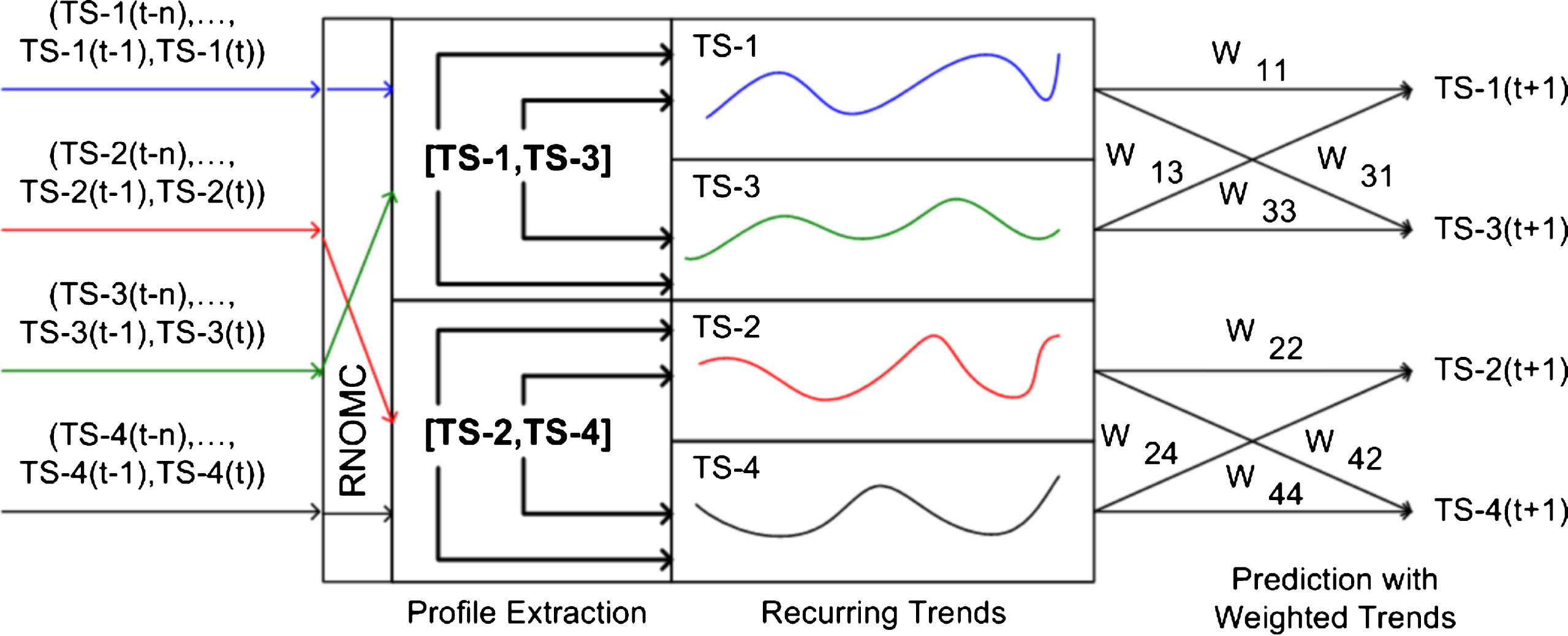
Step 6: calculate next value of x⁽ⁱ⁾ using the j found cluster centres of recurring trends, by giving more weight w to cluster centres that are closer to $w_{t}^{(i)}$ . Note: in this methodology cluster centres c_j of recurring trends represent trends of movement of time-series in a particular profile. The weight w_i,j that is assigned to cluster centre j when predicting the next value of x⁽ⁱ⁾ is calculated as follows: $w_{i, j} = \frac{max (D) - (D_{i, j} - min (D))}{max (D)},$ (12) where max(D) and min(D) are the maximum and minimum values of distance vector D = (D_i,1, D_i,2, . . . , D_i,j). In addition, next value of x⁽ⁱ⁾ is given by: $x_{t + 1}^{(i)} = \frac{\sum_{m = 1}^{j} w_{i, m} c_{m}}{\sum_{m = 1}^{j} w_{i, m}} .$ (13)

Fig.5

Time-series prediction using the repository profiles of movement and their related recurring trends (Widiputra, Pears, & Kasabov, 2012).

4. Indonesia sectoral indexes movement profiling

Today’s stock exchange markets are characterized by interdependencies demonstrating contagious behavior in different periods of time between listed stocks that are traded within the market it self and often being influenced by external financial condition as well. In relation to this, the existence of interaction or co-movement between a collection of stocks in a particular market has been significantly researched in the past few years. Accordingly, we have experience an increasing number of studies that are dedicated to address the effects of such interrelationships, along with the challenge of relationship identification and modeling.

However, most of the studies do not appear to utilize any methodology that is capable of simultaneously capturing and modeling dynamic profiles of movement between a collection of stocks in a stock exchange market (Patel, Shah, Thakkar, & Kotecha, 2010; Adebiyi, Adewumi, & Ayo, 2014; Kazem, Sharifi, Hussain, Saberi, & Hussain, 2013; Park & H., 2013). This actuality serves as the basis to why this study is looking at the possibility of implementing the LTM to extract such profiles. Therefore, in this study financial data of sectoral indexes in the Indonesia stock exchange market is used as a case study.

The financial data set observed in this setting includes a collection of time-series indexes of nine sectoral indexes in the Indonesia stock exchange market collected from the Yahoo!Finance (2017). Each of these sectoral indexes is consisting of a set listed stocks that are belong to similar category. The nine sectors are: 1) Agriculture sector (AGRI); 2) Basic Industry sector (BIND); 3) Construction sector (CONS); 4) Finance sector (FINA); 5) Infrastructure sector (INFA); 6) Mining sector (MING); 7) Manufacturing sector (MNFG); 8) Property sector (PROP); and 9) Trading sector (TRAD), in which their daily indexes, spanning 247 trading days from January 2016 to December 2016 are considered here.

Findings from previous researches which revealed that a set of stocks from the same sector often move simultaneously in similar manner (Ghosh & Kanjilal, 2016; Huang, H. An, & Huang, 2016; Yilmaz, Sensoy, Ozturk, & Hacihasanoglu, 2015; Bunn & Shiller, 2014; Dewandaru, Rizvi, Masih, Masih, & Alhabshi, 2014) become the main reason for the use of sectoral indexes instead of the individual stock values as a reference for the extraction of profiles of movement in this study. It is expected that the exploited methodology is capable of revealing and modeling the profiles of co-movement between these sectoral indexes. Having such knowledge would then benefit the financial analysts or fund managers to understand better the behavior of the Indonesia stock exchange market in particular and thus would help them in planning and making any investment decision.

Figure 6 depicts the trajectories of the nine sectoral indexes in the period of examination where it can be briefly recognized that the whole sectoral indexes are in general retaining similar trend of movement. Yet, a closer observation would disclose that detail movement of some sectors are more similar in comparison to the other. Therefore, the study aims to be able to unveil such profiles of co-movement by incorporating the adaptive clustering method for time-series profiling.

Fig.6

Daily indexes of 9 sectoral indexes in the Indonesia stock exchange market spanning 247 trading days from January 2016 to December 2016.

Additionally, throughout the conducted experiment the analyzed data set is divided into two different parts, i.e. the training part that consists of the first 173 points of the daily sectoral indexes; and the testing part that consists of the remaining 74 points from the complete set of 247 points. The conducted analysis employs an incremental testing process, which means that whenever a new instance arrives, a new profile of movement is to be identified and modeled before the prediction is and finally for the new instance to be added into the training set as an additional training example.

4.1. Extracted profiles of movement

The experiment in this study is conducted by dividing the nine sectoral indexes time-series data into two different parts, which are the training data and the testing data. Training data is used to examine the LTM capability to extract profiles of movement and build the knowledge repository from the observed collection of time-series data. In addition, the testing data is utilized for evaluating the methodology potential to incrementally learn and adjust it’s knowledge repository when new natures of profiles of movement are emerging and identified while preserving information about previously extracted profiles that are relatively unwavering. Here, the first 173 time-points of the complete collection of time-series data are defined as the training set, whilst the remaining are used for incremental profiling and evaluation, i.e. testing set.

Figure 7 reveals the extracted profiles of movement from the first 173 time moments of the nine sectoral indexes of the Indonesia stock exchange market that are identified by the profiling method. In Figure 7, each sector is represented by a numeric value defined as follows: #1: Agriculture (AGRI); #2 Basic Industry (BIND); #3 Construction (CONS); #4 Finance (FINA); #5 Infrastructure (INFA); #6 Mining (MING); #7 Manufacturing (MNFG); #8 Property (PROP) and #9 Trading (TRAD). Accordingly, Table 1 outlines the summary of profiles of movement extracted during the training period for the nine sectoral indexes.

Fig.7

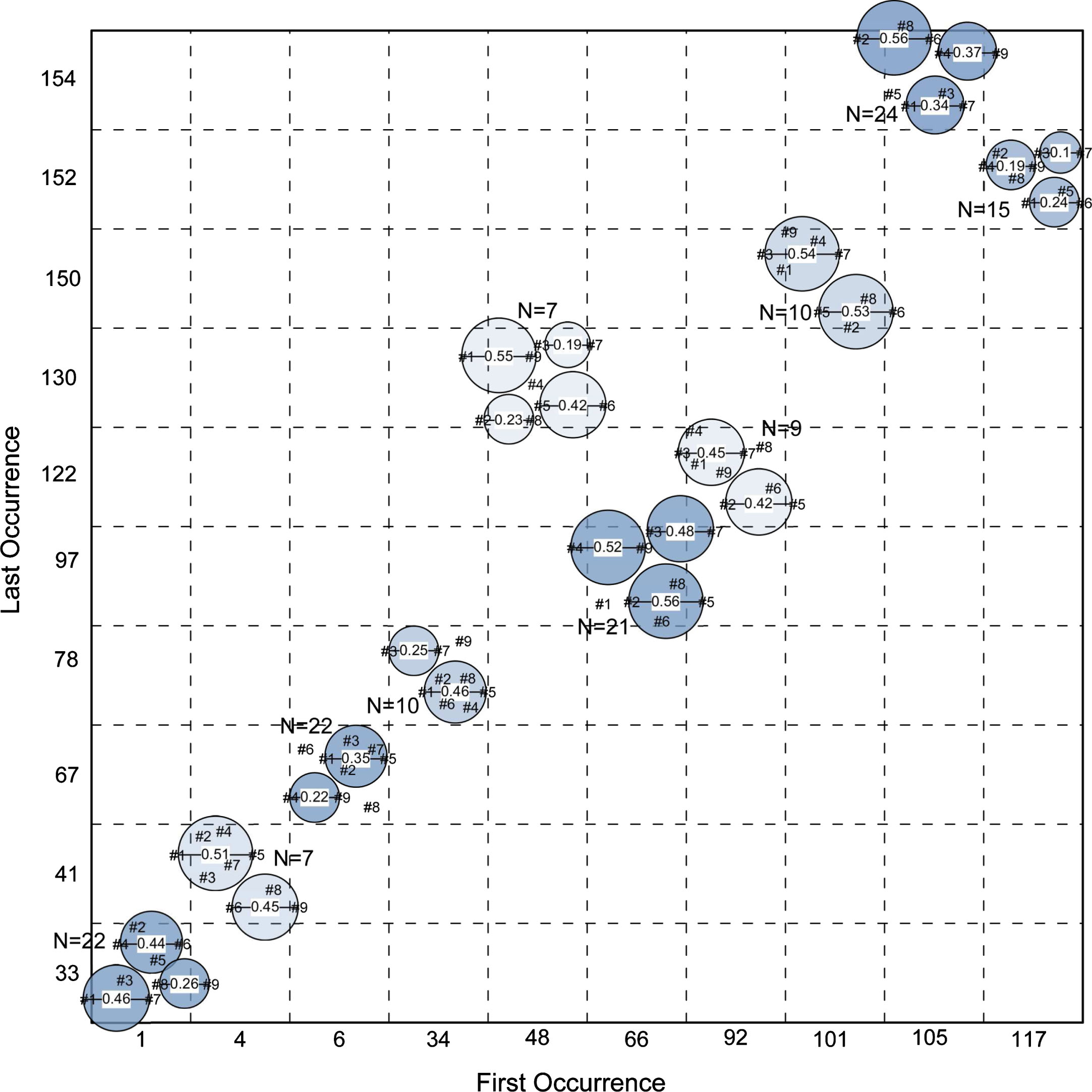
Extracted profiles of movement after data of nine sectoral indexes is conferred to LTM. The number #1, #2, #3, #4, #5, #6, #7, #8 and #9 represent the AGRI, BIND, CONS, FINA, INFA, MING, MNFG, PROP and TRAD sector respectively.

Table 1

Summary of extracted profiles of movement from the Indonesia stock exchange market sectoral indxes during training period (January 2016 to September 2016)

No	Profiles	Occurrence	Time Locality
1	[1 ;3 ; 7] , [2 ; 4 ;5 ; 6] , [8 ; 9]	22	1, 2, 3, 7, 8, 9, 16, 17, 18, 19, 20, 21, 22, 23, 24, 25, 26, 27, 28, 29, 32, 33
2	[1 ;2 ; 3 ;4 ; 5 ;7] , [6 ; 8 ;9]	7	4, 5, 37, 38, 39, 40, 41
3	[1 ;2 ; 3 ;5 ; 7] , [4 ; 9] , [6] , [8]	22	6, 10, 11, 12, 13, 14, 15, 30, 31, 44, 45, 46, 47, 49, 53, 54, 55, 56, 57, 58, 66, 67
4	[1 ;2 ; 4 ;5 ; 6 ;8] , [3 ; 7] , [9]	19	34, 35, 36, 42, 43, 51, 52, 59, 60, 61, 62, 63, 64, 65, 74, 75, 76, 77, 78
5	[1 ;9] , [2 ; 8] , [3 ; 7] , [4] , [5 ; 6]	7	48, 50, 68, 69, 116, 129, 130
6	[1] , [2 ; 5 ;6 ; 8] , [3 ; 7] , [4 ; 9]	21	66, 67, 70, 71, 72, 73, 79, 80, 81, 82, 83, 84, 85, 86, 87, 88, 89, 90, 91, 95, 97
7	[1 ;3 ; 4 ;7 ; 9] , [2 ; 5 ;6] , [8]	9	92, 93, 94, 96, 98, 99, 100, 121, 122
8	[1 ;3 ; 4 ;7 ; 9] , [2 ; 5 ;6 ; 8]	10	101, 102, 103, 104, 144, 145, 147, 148, 149, 150
9	[1 ;3 ; 7] , [2 ; 6 ;8] , [4 ; 9] , [5]	24	105, 106, 107, 108, 109, 110, 111, 112, 113, 114, 115, 123, 124, 125, 126, 127, 128, 131, 135, 136, 137, 151, 153, 154
10	[1 ;5 ; 6] , [2 ; 4 ;8 ; 9] , [3 ; 7]	15	117, 118, 119, 120, 132, 133, 134, 138, 139, 140, 141, 142, 143, 146, 152

The circles in Figure 7 are representing profiles of movement between series captured from the analyzed data set, where cluster radius represents the state of dissimilarity between series that belong to identical cluster or profile while relative positioning of the labels indicates the degree of similarity in their behavior. For instance, from the circle plotted at coordinate (1, 33) it can be seen that series #3 is positioned closer to #7 than to #1. This indicates that the movement of the Construction sector is more similar to the movement of the Manufacturing sector and therefore they possess higher degree of correlation in comparison to that of the Construction sector and the Agriculture sector.

The color of a circle signifies the number of occurrences of a particular profile of movement. Darker color indicates that a significant number of occurrences has been identified along the profiling process. Additionally, the exact number of occurrences of a particular profile is also given by N. Furthermore, the x-axes represents the initial time moment when a particular profile emerged, while the y-axes represents the last time moment when a particular profile of movement was recognized and captured.

Figure 1 and Table 1 reveal that the Construction and Manufacturing sectors are closely related and that they are trajecting together continuously in significant interval of time moments. This piece of worthy information is discovered by analyzing the circles plotted at coordinate (34, 78), (48, 130), (66, 97), and (117, 152) in Figure 1 and also the reality as outlined in Table 1 in which both sector always belong to the same set of profiles during the evaluation period. Consequently, the small radius of plotted circle indicates that the correlation between both sectors is very high. This finding points out that in the period under evaluation, the Construction and Manufacturing sectors are frequently and continuously moving in a similar fashion.

Furthermore, both Figure 7 and Table 1 disclose that even though the structure of profiles of movement is changing over time, the Construction and Manufacturing sectors maintain their closeness constantly. This finding signifies the existence of resilient relationship, in terms of co-movement, between both sectors. The discovery might be used as a suggestion to explain the association between Construction and Manufacture sectors. As the Construction sector moves toward a positive direction, the Manufacturing sector would immediately follows and vice versa. This actuality confirms the natural bond of both sectors where construction works require products from manufacturer and consequently the Manufacturing sector would definitely grow as they receive more requests from the Construction sector.

Morevover, Figure 7 and Table 1 be evidence for the existence of some episodes when the Agriculture sector and the Construction sector are moving separately, the image and Table 1 also reveal that there exists a number of significant periods when both sectors are closely related and progressing together in a similar manner, i.e. Profile #1, #2, #3, #7, #8 and #9 from Table 1. Another discovery that can be induced from Figure 7 is that generally we can learn that the Infrastructure sector and also the Trading sector have a tendency to shift reciprocally with the other sectors during the period of evaluation.

Based on the analysis that can be inferred from Figure 7 and Table 1 as they are outlined above, some conclusions in relation to the extraction of profiles of movement from the observed 9 sectoral indexes can be made as follows:

The Construction sector is more likely to move in a similar fashion with the Manufacturing sector and therefore can be considered as possessing more noteworthy association compared to the other sectors;

There exists a period at the start of the observation period when the Property sector is moving in a similar course with the Trading sector, i.e. Profile #1 in Table 1. Yet, there is also a significant number of episodes (towards the end of the observation period) when the two series are tend to progress individually, i.e. Profile #6, #7, #8, #9. Conversely, the association between both sectors is restored in the final period of observation, i.e. Profile #10. This finding suggest that profiles of co-movement between series are changing dynamically over time and can only be captured by an adaptive method;

During the observation period, the relationships, in terms of co-movement, between the Agriculture sector and the Property sector are more momentous when compared to the association between them and the other sectors as it can be seen in Profile #4 from Table 1. These finding indicates that these three sectors have higher behavioral attachments when compared to the other sectors.

These inferences are in agreement both with the trajectories of the nine series, as illustrated in Figure 6, and therefore suggest the LTM capability to dynamically capture, model and maintain profiles of movement from a collection of time-series over time.

To prove that the extracted profiles of movement are in reality represents the hidden manners of the observed system and to also confirm that they can be exploited as knowledge to predict the behavior of the observed system, we exploited the constructed knowledge repository to restore trajectories of the nine sectoral indexes in the training period.

Both Figure 8 and Figure 9 illustrate the reconstructed trajectories calculated by the utilized method based on the profiles of movement that have been extracted. It is clearly seen that the reconstructed trajectories produced by the algorithm match closely with the actual trajectories. This outcome proves that being able to extract profiles of movement from a collection of time-series data can be of help to understand the nature of observed dynamic system and further help to mimic or forecast its future behavior.

Fig.8

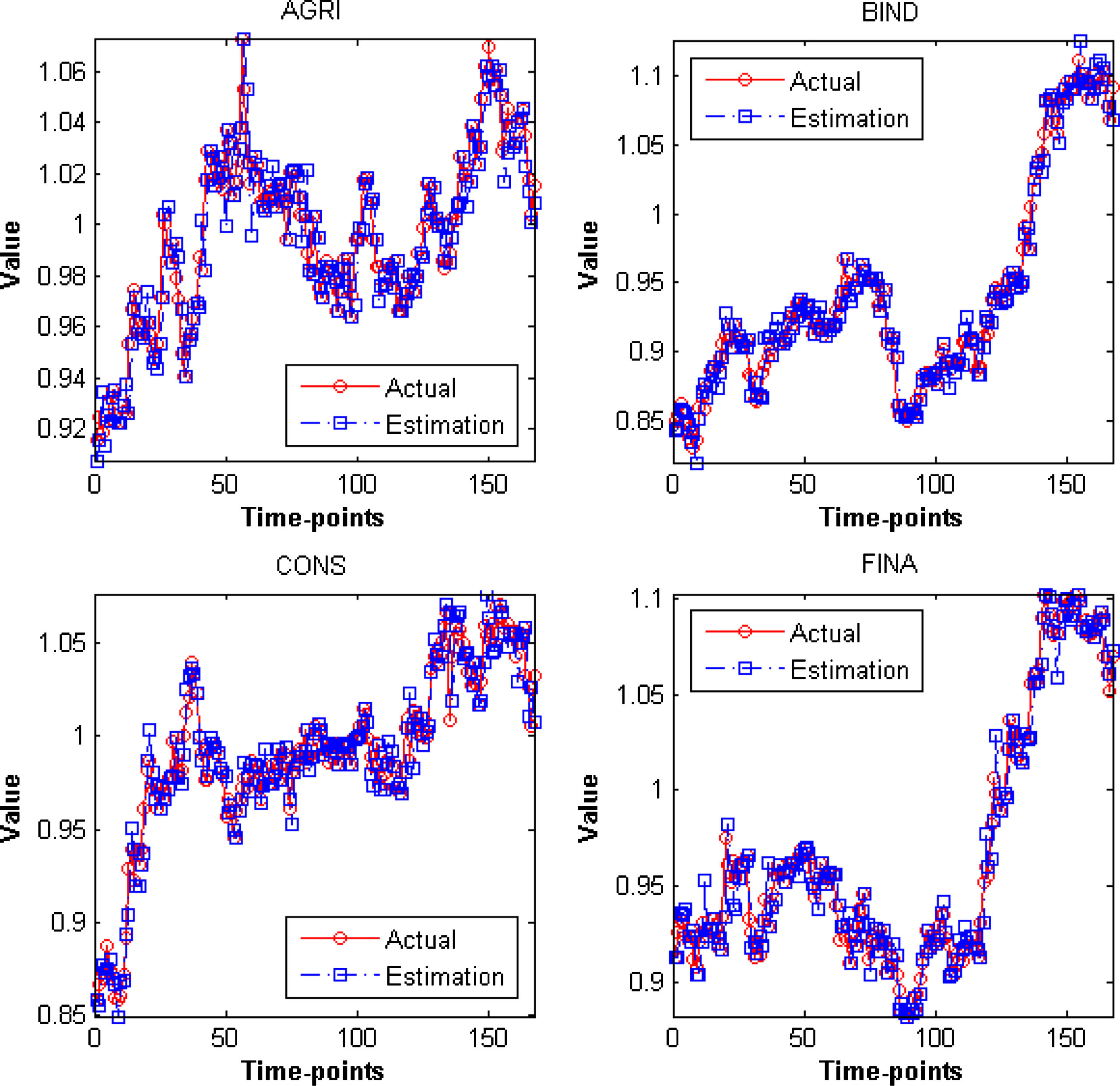
Plot of estimated trajectories of the Agriculture (AGRI), Basic Industry (BIND), Construction (CONS) and Financial (FINA) sector of the Indonesia Stock Exchange Market for the first 173 time moments of the period January 2016 to December 2016.

Fig.9

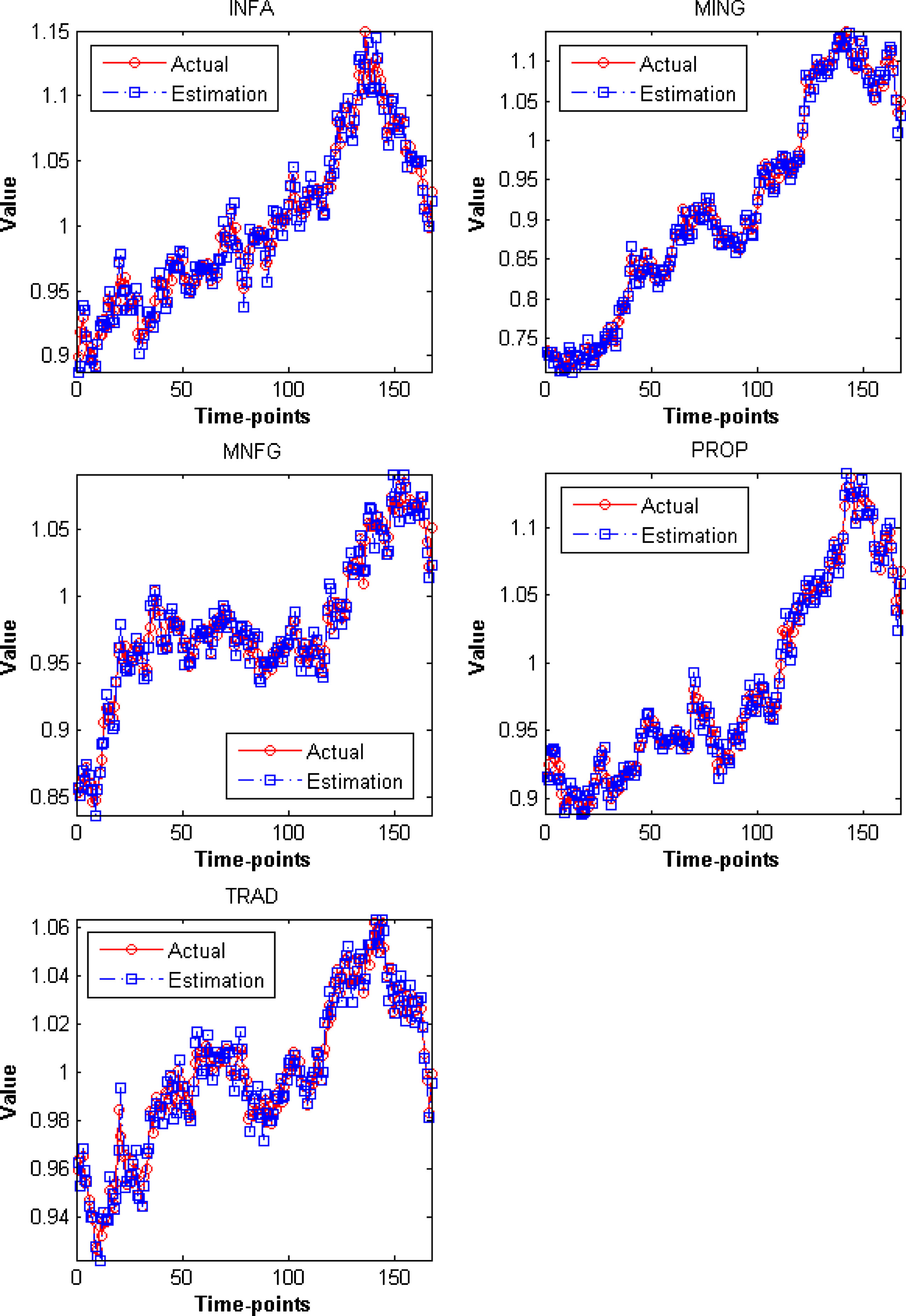
Plot of estimated trajectories of the Infrastructure (INFA), Mining (MING), Manufacturing (MNFG), Property (PROP) and Trading (TRAD) sector of the Indonesia Stock Exchange Market for the first 173 time moments of the period January 2016 to December 2016.

4.2. Prediction of the Indonesia Sectoral Indexes

Figure 10 and Figure 11 show that the predictions made by utilized methodology, based on the calculation that exploit the repository of profiles of movement, are considerably closely match the actual trajectories of the nine under observation sectoral indexes in the Indonesia stock exchange market. These figures also suggest that the repository of profiles of movement and the proposed prediction algorithm that make use of it enable the creation of reliable model that can be operated for predicting movement of the observed sectoral indexes across the whole period of examination.

Fig.10

Plot of estimated trajectories of the Agriculture (AGRI), Basic Industry (BIND), Construction (CONS) and Financial (FINA) sector of the Indonesia Stock Exchange Market for the last 74 time moments of the period January 2016 to December 2016.

Fig.11

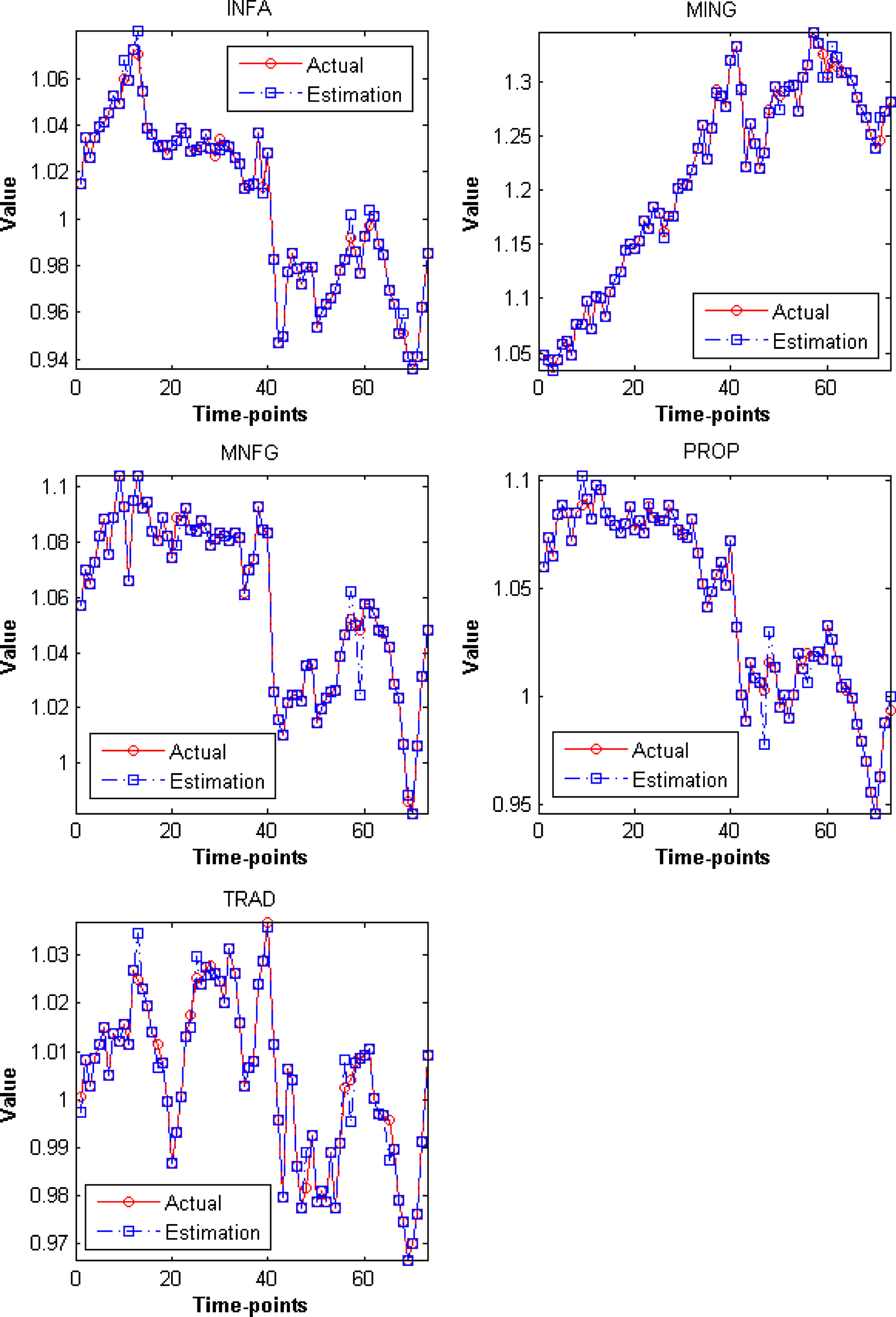
Plot of estimated trajectories of the Infrastructure (INFA), Mining (MING), Manufacturing (MNFG), Property (PROP) and Trading (TRAD) sector of the Indonesia Stock Exchange Market for the last 74 time moments of the period January 2016 to December 2016.

Additionally, to confirm that conducting the prediction of future values for a collection of time-series by simultaneously incorporating their profiles of movement offers better prediction accuracy, a comparison with other predictions for equal setting made by Multiple Linear Regression (MLR), Multi Layer Perceptron (MLP) and random walk methods is conducted in this study. The random walk model is a method for time-series analysis, which simply assume that the upcoming value of a series is equal to it’s current value. In this study, the random walk without drift model defined simply by Equation 1 is used while prediction made by MLR and MLP is calculated by making use of the NeuCom software (Engineering & Institute, 2017). $x_{t + 1} = x_{t}$ (14)

In some cases, the random walk model might perform better in predicting trajectories of a time-series, i.e. in terms of sum squared residual. Yet, this model is famous for producing shadow plot of the series under observation, lagging exactly one time-step behind and therefore does not make any contribution to the extraction and modeling of knowledge on the observed system. It is because, the methodology simply assumes that the upcoming value is exactly the same as current value.

Table 2 shows the much smaller Root Mean Squared Error (RMSE) of the LTM in comparison to the other traditional methods when being applied for the prediction of observed nine sectoral indexes. This results clearly indicates the value of simultaneously extracting and exploiting profiles of movements between from a collection of time-series in maintaining the quality of time-series prediction accuracy.

Table 2

Comparison of the Localized Trend Model (LTM) prediction error rates against the MLR, MLP and random walk model, in RMSE

No	Variable	LTM	MLR	MLP	Random Walk
1	AGRI	0.009	0.580	0.441	1.663
2	BIND	0.014	0.727	0.43	1.341
3	CONS	0.014	0.639	0.572	1.474
4	FINA	0.012	0.190	0.29	1.456
5	INFA	0.012	0.380	0.144	1.634
6	MING	0.020	0.277	0.143	1.419
7	MNFG	0.013	0.439	0.357	1.447
8	PROP	0.013	0.890	0.729	1.436
9	TRAD	0.009	0.290	0.129	1.451

5. Conclusion and future work

The study presented an utilization of methodology to recognize and model profiles of movement from a collection of time-series data, which also captured recurring trends that take place in each identified profile. The recurring specific behavior in this methodology is described as recurring profiles of co-movement between pairs of series that influence each other is a specific time locality.

Experimental results and analysis on data set of the Indonesia stock exchange market sectoral indexes confirms the developed algorithm capability to extract significant time-varying profiles of movement along with the recurring trends. Moreover, this repository of profiles of movement can be continuously updated as new profiles are emerging when recent observations from the dynamic system of interest become available.

Additionally, the experimentation on the Indonesia stock exchange market sectoral indexes data set undoubtedly prove that the utilized adaptive clustering method demonstrates the ability to:

Extract profiles of movement and recurring trends from a collection of time-series data;

Identify assembly of sectoral indexes in the Indonesia stock exchange market that exhibit the drift to progress collectively;

Perform simultaneous prediction of a time-series collection with excellent precision as it is proofed by the forecasting results of the Indonesia stock exchange sectoral indexes values;

Evolve, by continuing to extract profiles of movement and recurring trends over time when new data samples become available.

A further direction related to the refinement of this approach is to explore the use of correlation analysis methods that are capable of detecting non-linear correlations between observed variables, i.e. correlation ratio, Copula, etc., in the process of extracting the profiles of movement from a collection of time-series data originating from a particular dynamic system.

Footnotes

Acknowledgement

This research is funded in part by the Ministry of Research, Technology and Higher Education of the Republic of Indonesia, under Research Grant No. 0440/ K3/KM/2017.

References

Adebiyi, A., Adewumi, A., Ayo, C.2014. Comparison of arima and artificial neural networks models for stock price prediction. Journal of Applied Mathematics. DOI: 10.1155/2014/614342

Aghabozorgi, S., Shirkhorshidi, A., Wah, T.2015, October. Time-series clustering-a decade review, Information Systems53, 16–38.

Bakoben, M., Bellotti, T., Adams, N.2015, January.Learning segmentation from time series clustering. In Proceedings of conference on computational mathematics, computational geometry & statistics (cmcgs) pp. 61–67.

Bunn, O., Shiller, R.2014. Changing times, changing values: A historical analysis of sectors within the us stock market 1872-2013 (no. w20370). National Bureau of Economic Research. http://www.nber.org/papers/w20370

Cevikalp, H., Polikar, R.2008. Local classifier weighting by quadratic programming, IEEE Transactions on Neural Networks19(10), 1832–1838.

Chen, T., Lee, S.2015, April. A weighted ls-svm based learning system for time series forecasting, Information Sciences299, 99–116.

Dewandaru, G., Rizvi, S., Masih, R., Masih, M., Alhabshi, S.2014. Stock market co-movements: Islamic versus conventional equity indices with multi-timescales analysis, Economic System38(4), 553–571.

Engineering, A.K., Institute, D.R.2017. Neucom. https://kedri.aut.ac.nz/areas-of-expertise/data-mining-and-decision-support/neucom

Fernandez, F., Kerre, E., Jimenez, B.2016. A global fuzzy model for non linear systems using interval valued fuzzy sets, Ingenieria Electronica, Automatica & Comunicaciones37(3), 50–57.

10.

Freund, R., Wilson, W., Sa, P.2006. Academic Press.

11.

Ghosh, S., Kanjilal, K.2016, January.Co-movement of international crude oil price and indian stock market: Evidences from nonlinear cointegration tests, Energy Economics53, 111–117.

12.

Huang, S.H., An, X. G., Huang, X.2016, January.Timefrequency featured co-movement between the stock and prices of crude oil and gold, Physica A: Statistical Mechanics and its Applications, 444, 985–995.

13.

Islam, M., Yao, X., Nirjon, S., Islam, M., Murase, K.2008. Bagging and boosting negatively correlated neural networks, IEEE Transactions on Systems, Man, and Cybernetics, Part B (Cybernetics)38(3), 771–784.

14.

Kasabov, N.

2007. Global, local and personalised modeling and pattern discovery in bioinformatics: An integrated approach, Pattern Recognition Letters28(6), 673–685.

15.

Kasabov, N., Pang, S.2003, December. Transductive support vector machines and applications in bioinformatics for promoter recognition. InProceedings of ieee international conference on neural networks and signal processing pp. 1–6.

16.

Kasabov, N., Song, Q.2002. Denfis: Dynamic evolving neural-fuzzy inference system and its application for time-series prediction, IEEE transactions on Fuzzy Systems10(2), 144–154.

17.

Kazem, A., Sharifi, E., Hussain, F., Saberi, M., Hussain, O.2013. Support vector regression with chaos-based firefly algorithm for stock market price forecasting, Applied Soft Computing13(2), 947–958.

18.

Kourentzes, N., Barrow, D., Crone, S.2014. Neural network ensemble operators for time series forecasting, Expert Systems with Applications41(9), 4235–4244.

19.

Langkvist, M., Karlsson, L., Loutfi, A.2010, June.A review of unsupervised feature learning and deep learning for time-series modeling, Pattern Recognition Letters42, 11–24.

20.

Nadaraya, E.

1964. On estimating regression, Theory of Probability & Its Applications9(1), 141–142.

21.

Park, K., H., S.

2013. Stock price prediction based on a complex interrelation network of economic factors, Engineering Applications of Artificial Intelligence26(5), 1550–1561.

22.

Patel, J., Shah, S., Thakkar, P., Kotecha, K.2010. Predicting stock and stock price index movement using trend deterministic data preparation and machine learning techniques, Expert Systems with Applications42(1), 259–268.

23.

Pears, R., Widiputra, H., Kasabov, N.2013. Evolving integrated multimodel framework for on line multiple time series prediction, Evolving Systems4(2), 99–117.

24.

Rodrigues, P., Gama, J., Pedroso, J.2008. Hierarchical clustering of time-series data streams, IEEE Transactions on Knowledge and Data Engineering20(5), 615–627.

25.

Shapiai, M., Ibrahim, Z., Khalid, M., Jau, L., Pavlovich, V.2010, July.A non-linear function approximation from small samples based on nadaraya-watson kernel regression, In Proceedings of ieee computational intelligence, communication systems and networks (cicsyn) pp. 28–32.

26.

Song, Q., Kasabov, N.2001. November.Ecm-a novel on-line, evolving clustering method and its applications, Foundations of Cognitive Science, 631–682.

27.

Wang, L., Zeng, Y., Chen, T.2015. Back propagation neural network with adaptive differential evolution algorithm for time series forecasting, Expert Systems with Applications42(2), 855–863.

28.

Watson, G.

1964. Smooth regression analysis. Sankhya: The Indian Journal of Statistics, Series A, 359–372.

29.

Widiputra, H.

2014. Dynamic interaction network to model cointegration in idx leading stocks, Advanced Science Letters20 (10-11), 1900–1904.

30.

Widiputra, H., Pears, R., Kasabov, N.2011a. Dynamic interaction networks versus local trend models for multiple time-series prediction, Cybernetics and Systems: An International Journal42(2), 100–123.

31.

Widiputra, H., Pears, R., Kasabov, N.2011b. Multiple time-series prediction through multiple time-series relationships profiling and clustered recurring trends, Advances in Knowledge Discovery and Data Mining, LNCS 3365, 161–172.

32.

Widiputra, H., Pears, R., Kasabov, N.2012. Dynamic learning of multiple time series in a nonstationary environment, Learning in Non-Stationary Environments, SpringerNew York, 303–347.

33.

Yamada, T., Yamashita, K., Ishii, N., Iwata, K.2006, June. Text classification by combining different distance functions with weights. In Proceedings of ieee software engineering, artificial intelligence, networking, and parallel/distributed computing pp. 85–90.

34.

Yilmaz, M., Sensoy, A., Ozturk, K., Hacihasanoglu, E.2015, April. Cross-sectoral interactions in islamic equity markets, Pacific-Basin Finance Journal32, 1–20.