Machine learning and corporate bond trading

Abstract

We demonstrate how machine learning based recommender systems can be effectively employed by market makers to filter the information embedded in Requests for Quote (RFQs) to identify the set of clients most likely to be interested in a given bond, or, conversely, the set of bonds that are most likely to be of interest to a given client. We consider several approaches known in the literature and ultimately suggest the so-called latent factor collaborative filtering as the best choice. We also suggest a scalable optimization procedure that allows the training of the system with a limited computational cost, making collaborative filtering practical in an industrial environment.

Keywords

Machine learning Recommender systems Collaborative filtering Corporate bond trading

1. Introduction

In the corporate bond business, market makers need to handle large amounts of requests from clients, typically in the form of electronic inquiries - or Requests for Quote (RFQs) - and enter positions, assuming outright issuer risk. In some cases, those positions need to be closed quickly in order to minimize the associated market risk and balance sheet costs. When a position needs to be closed out, sales teams contact clients who may be interested in taking over that position. However, since it is generally possible to contact only a very small fraction of the dealer’s clients, it is of paramount importance for salespeople to be intimately familiar with the clients’ trading preferences.

This is particularly challenging because, at any given time, most of the market activity is concentrated on a small number of bonds while trading on the majority of the inventory happens fairly infrequently. This is known as the long-tail problem. In this situation an effective recommender systems (RS), that is an algorithm able to identify the small population of clients that are most likely to be interested in a given bond, could bring substantial value to the dealer and, by virtue of providing a better service, to its clients.

Similar problems are not uncommon in many other industries. A common challenge of e-Commerce websites is helping customers sort through a large variety of offered products to easily find the ones they are most interested in. Music and video streaming services, like Netflix or Spotify, are equipped with algorithms which aim at personalized recommendations to their users to improve their experience. One of the tools commonly employed for these tasks are RS (Goldberg et al., 1992; Linden et al., 2003).

In this paper, we investigate the application to corporate bond trading of RS based on machine-learning techniques able to use the information embedded in RFQs. Two main categories of models are described: content-based filtering and collaborative filtering, along with approaches to training and testing that we trialed on example data. We also suggest a few practical optimizations that are essential for reducing the time necessary to train the algorithms at a level that makes their usage viable in an industrial setting.

2. Bond recommender systems

Broadly speaking, RS fall into two categories, content-based and collaborative filtering, differing in their interactions with users, the agents we would like to make recommendations to, and items, the set of objects we need to recommend. Content-based filtering (CBF) methods (Lops et al., 2011) create profiles for users and items in order to characterize their nature and then try to match the user-item pairs using metrics based on the similarity between profiles. In the context of the bond market making business, each bond can be characterized by a set economic features and each client can be characterized by the features of the bonds they have been historically interested in. Collaborative filtering (CF) (Goldberg et al., 1992), instead, only employs past user behavior in order to detect users with similar preferences over items. For example, in the specific context, by knowing what bonds clients have historically inquired, one can infer the interdependencies among clients and bonds and thus find potential associations for new client-bonds pairs.

2.1. Content-based filtering

In general, CBF models assume that clients are looking for bonds with certain economic characteristics or features. For example, some clients are more likely to trade long-dated bonds within certain industries. Based on this idea, the profile of the clients can be represented by the features of previously traded bonds. If bond i has similar features to those traded by client u, then it makes sense to recommend bond i to client u. This can be formalized as follows.

Each bond is characterized by a set of categorical features (e.g. Region, Industry, Coupon Type) and numerical features (e.g. Maturity, Yield, Credit Rating). We indicate with $y$ ⁱ = [ $C$ ⁱ; Nⁱ] ^t the set of features for bond i, i = 1, …, N, where $C^{i} = [C_{1}^{i}, \dots, C_{n_{c}}^{i}]^{t}$ is the vector of categorical features and $N^{i} = [N_{1}^{i}, \dots, N_{n_{n}}^{i}]^{t}$ , with $N_{k}^{i} = [N_{k 1}^{i}, \dots, N_{{kn}_{b}}^{i}]^{t}$ , is the matrix of numerical features. Here n_c and n_n are the number of categorical and numerical features, respectively, and n_b is the number of intervals in which the domain of numerical features is discretized into. For each bond i, the entries of the vector $C$ ⁱ correspond to the categorical features characterizing the bond (e.g. Region: European, Industry: Financial, Coupon Type: Fixed), encoded as strings. This gives a more concise representation compared to transforming categorical data to a numerical binary representation (Huang, 1997, 1998). For each vector $N_{k}^{i}$ , k = 1, …, n_n, only the single entry corresponding to the interval in which the bond’s k-th feature falls into is equal to one, while the remaining n_b - 1 components are set to zero.

Similarly, we indicate with $x$ ^u = [ $C$ ^u; N^u] ^t the set of features for client u, u = 1, …, M. In this case, for each vector $N_{k}^{u}$ , k = 1, …, n_n, the entry $N_{kl}^{u}$ is set to the frequency of bonds with the k-th feature falling in the l-th interval, as observed in the historical sample of RFQs. Each entry of the vector $C$ ^u is set to the most commonly observed categorical feature.

A simple way to use such data to make recommendations is to compute the predicted preference of client u for bond i, ${\hat{p}}_{ui}$ , as a pseudo inner product of the client profile vector $x$ ^u and the bond features vector $y$ ⁱ. We define this pseudo inner product as

${\hat{p}}_{ui} \equiv \sum_{k = 1}^{n_{c}} C_{k}^{u} C_{k}^{i} + \sum_{k = 1}^{n_{n}} N_{k}^{u} \cdot N_{k}^{i},$ (1) where we have used the notation

$C_{k}^{u} C_{k}^{i} \equiv δ (C_{k}^{u}, C_{k}^{i}),$ (2) with δ (a, b) the generalized Kronecker delta. This is equal to 1 if a = b (for any type a and b, including strings as in this case), and zero otherwise. The estimator above assumes all the features are of equal importance. A more accurate estimator can be obtained by weighting each of the features in (14) and computing the following weighted pseudo inner product:

$(x^{u} \circ y^{i})^{t} w^{u} \equiv \sum_{k = 1}^{n_{c}} w_{k}^{u} C_{k}^{u} C_{k}^{i} + \sum_{k = 1}^{n_{n}} w_{n_{c} + k}^{u} N_{k}^{u} \cdot N_{k}^{i},$ (3) where ∘ is the element-wise product and $w^{u} = [w_{1}^{u}, \dots, w_{n_{f}}^{u}]^{t}$ , with n_f = n_n + n_c, is the feature weight vector for client u. Given the clients’ and the bonds’ features, the objective is to find the optimal weights $w_{k}^{u}$ for each client u. This leads to the ridge regression (Hastie et al., 2009) based content filtering:

$min_{w^{u}} \sum_{u, i} c_{ui} (p_{ui} - (x^{u} \circ y^{i}) \cdot w^{u})^{2} + λ_{reg} | | w^{u} | |^{2} .$ (4) Here, following (Hu et al., 2008) the preference of client u for bond i, given the historical sample of RFQs in a given time horizon, p_ui, is defined as the binary variable

$p_{ui} = {\begin{matrix} 1 if client u traded bond i \\ 0 otherwise . \end{matrix}$ (5) The confidence we have in such preference, c_ui, is defined as

$c_{ui} = 1 + α r_{ui},$ (6) where r_ui is given by the total notional traded by client u in bond i, and α is an adjustable parameter.

By differentiation, the set of weights minimizing Equation (1) reads:

$w^{u} = (A^{u})^{- 1} B^{u},$ (7) where

$\begin{matrix} A_{lm}^{u} & = x_{l}^{u} x_{m}^{u} \sum_{i = 1}^{N} c_{ui} y_{l}^{i} y_{m}^{i} + λ_{reg} δ_{lm}, \\ B_{l}^{u} & = x_{l}^{u} \sum_{i = 1}^{N} c_{ui} p_{ui} y_{l}^{i}, \end{matrix}$ and N is the number of bonds. After obtaining $w$ ^u, the preference of client u for bond i can be computed by:

${\hat{p}}_{ui}^{CBF} = (x^{u} \circ y^{i}) \cdot w^{u} .$ (8) For any client u, the larger ${\hat{p}}_{ui}$ , the more likely client u is to be interested in bond i.

2.2. Collaborative filtering

Contrary to CBF, collaborative filtering (CF) can be performed using only the information contained in the so-called user-item observations matrix (Hu et al., 2008). The entries in this matrix can be either user ratings for explicit feedback data or built from the preference and indicator matrices, Equations (14) and (15), for implicit data. Given the observed entries in such a matrix, different methods can be used to compute the missing ones.

2.2.1. Neighborhood models

The most common approach to CF is based on Neighborhood models (Hastie et al., 2009), which usually have two forms: user-oriented and item-oriented. User-oriented Neighborhood CF (U-NCF) models try to estimate the unknown preference of a client for a bond given the preferences of similar clients. Conversely, item-oriented Neighborhood CF (I-NCF) models use the information about a client’s preference for similar bonds.

Given the user-item observation matrix p_ui in Equation (14) for all client-bond pairs, the similarity between two bonds i and j can be computed as the following ‘cosine’ similarity:

$s_{ij} = \frac{\sum_{u} p_{ui} p_{uj}}{\sqrt{\sum_{u} p_{ui}^{2}} \sqrt{\sum_{u} p_{uj}^{2}}} .$ (9) Likewise, the similarity between two clients u and v can be computed as:

$s_{uv} = \frac{\sum_{i} p_{ui} p_{vi}}{\sqrt{\sum_{i} p_{ui}^{2}} \sqrt{\sum_{i} p_{vi}^{2}}} .$ (10)

After computing the pairwise similarity s_uv or s_ij for all clients and bonds, the missing preference of client u over bond i can be decided by finding either the top k most similar clients or most similar bonds. For example, denoting the set of the top k most similar bonds to bond i by S^k (i), the preference for client u over all bonds is:

${\hat{p}}_{ui}^{I - NCF} = \frac{\sum_{j \in S^{k} (i)} s_{ij} p_{uj}}{\sum_{j \in S^{k} (i)} s_{ij}} .$ (11) Similarly, denoting the set of the top k most similar clients to client u by ${\tilde{S}}^{k} (u)$ , the preference for client u over all bonds can also be estimated as

${\hat{p}}_{ui}^{U - NCF} = \frac{\sum_{v \in {\tilde{S}}^{k} (u)} s_{uv} p_{uj}}{\sum_{u \in {\tilde{S}}^{k} (v)} s_{uv}} .$ (12)

2.2.2. Latent factor models

The basic idea underlying latent factor models is the factorization of the client-bond observation matrix, p_ui, into a product of smaller matrices, which can be interpreted as the latent features for clients and bonds respectively, as depicted in Fig. 1. Following (Hu et al., 2008), this can be formulated as the following (non-convex) optimization problem

Fig. 1.

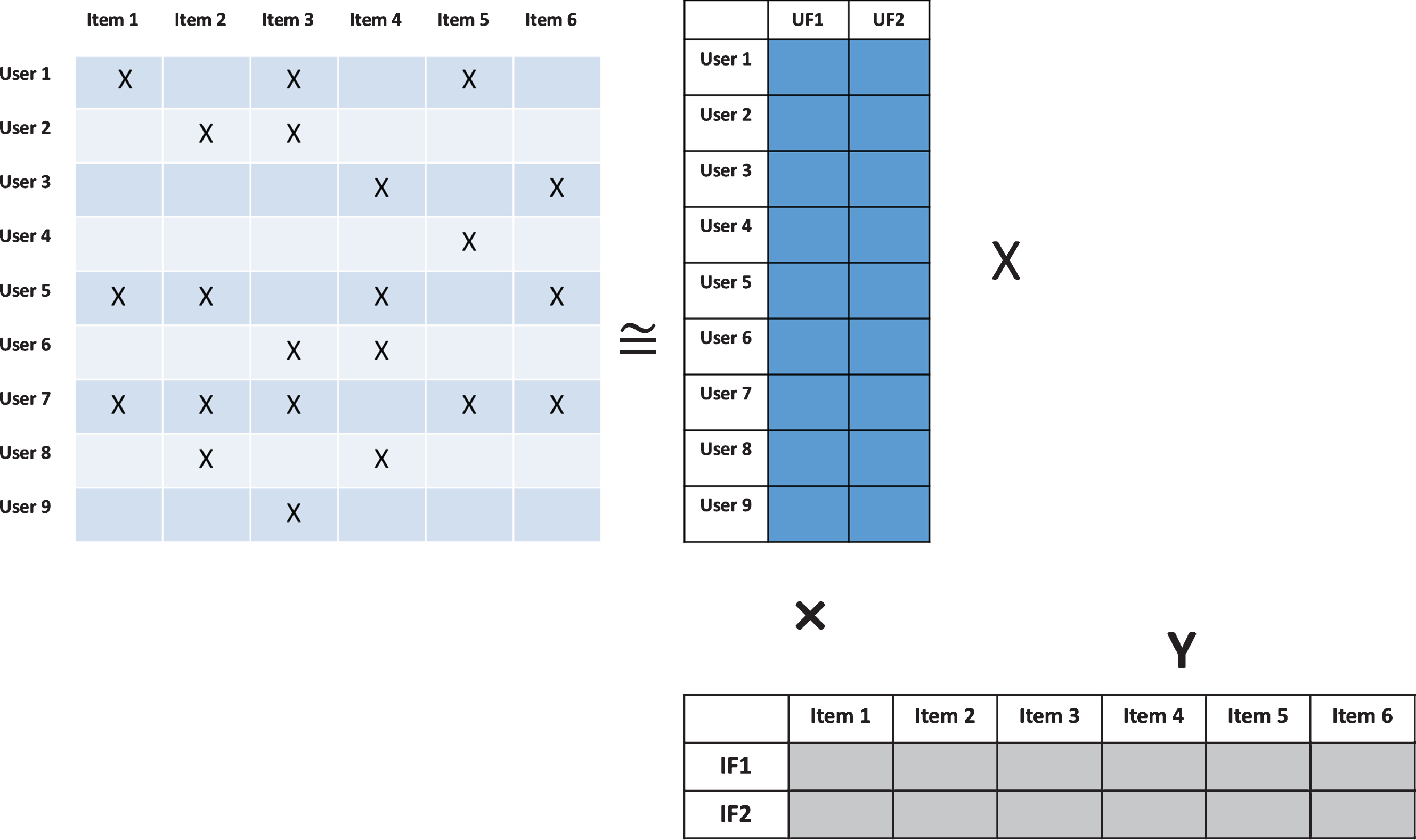
Illustration of matrix factorization for CF.

Fig. 2.

Example of ROC curve in red and AUC in grey. While the plot has been generated with simulated data, the results are indicative of the performance that can be expected from recommender systems in practice.

$min_{x, y} \sum_{u, i} c_{ui} (p_{ui} - x^{u} \cdot y^{i})^{2} + λ_{reg} (| | x^{u} | |^{2} + | | y^{i} | |^{2}),$ (13) where $x^{u} = [x_{1}^{u}, \dots x_{K}^{u}]^{t}$ and $y^{u} = [y_{1}^{i}, \dots y_{K}^{i}]^{t}$ are the K latent factors vectors for client u and the bond i, respectively and c_ui, p_ui and λ_reg are defined as in Equation (1).

A common approach to this optimization is the so-called Alternating-Least-Squares (ALS) (Hu et al., 2008), where the optimal user-factors are computed assuming that the item-factors are fixed and vice-versa until convergence. In this case: $y^{i} = (X^{t} C^{i} X + λ_{reg} I)^{- 1} X^{t} C^{i} p^{i}$ (14) $x^{u} = (Y^{t} {\tilde{C}}^{u} Y + λ_{reg} I)^{- 1} Y^{t} {\tilde{C}}^{u} {\tilde{p}}^{u}$ (15) where $X_{lm} = x_{m}^{l}$ , $Y_{lm} = y_{m}^{l}$ , $C_{lm}^{i} = δ_{lm} c_{li}$ , ${\tilde{C}}_{lm}^{u} = δ_{lm} c_{ul}$ , $p_{l}^{i} = p_{li}$ , ${\tilde{p}}_{l}^{u} = p_{ul}$ and I is the identity matrix in $ℝ^{K}$ . After computing $x$ ⁱ and $y$ ^u for a number of iterations until the desired degree of convergence is achieved, recommendations can be made using the metric ${\hat{p}}_{ui}^{LF} = x^{u} \cdot y^{i} .$ (16)

2.2.3. Implementation

The Latent Factor CF is significantly more computationally demanding than the other methods. As a result, to make the approach practical, it is important to optimize the computation of Eqs. (14) and (15). Firstly, one can avoid the matrix inversion and compute the solution of the linear systems by means of the Conjugate Gradient method (Hastie et al., 2009). This lowers the computational complexity per client or user (when using a standard matrix inversion) from $O (K^{3})$ to $O (m n)$ , where m is the number of non-zero entries in the matrix and n_I is the number of iterations for convergence. Secondly, a further optimization can be obtained by factorizing the matrices X^tCⁱX and Y^tC^uY. As explained in (Hu et al., 2008) this lowers the overall computational complexity per bond for calculating X^tCⁱX (resp.Y^tC^uY) from $O (K^{2} M)$ (resp. $O (K^{2} N)$ ) to $O (K^{2} (1 + N))$ (resp. $O (K^{2} (1 + M))$ ), where N_u (resp., M_i) is the number of nonzero elements in the matrix p_ui for client u (resp., for bond i). When applied across all bonds and clients this lowers the computational complexity of Eqs. (14) and (15) from $O (K^{2} MN + K^{3} (M + N) + KMN + K^{2} (M + N))$ to $O (K^{2} ((N + ℳ) + \sum_{u = 1}^{M} N_{u} + \sum_{i = 1}^{N} M_{i}) + m n_{I} (M + N) + K ℳ N)$ per iteration. Finally, as seen from Eqs. (14) and (15), the calculations for each client and each bond latent factors can be performed in parallel in a multi-threaded environment so that the training cost can be reduced by the number of threads available, which is currently of order 10 on a standard desktop computer. Our Cython

¹ http://cython.org/

based Python implementation was able to train the Latent Factor CF on our dataset within a few seconds on a desktop computer with commercially standard specifications.

3. Testing

A proportion of the RFQ data must be reserved for testing performance, we refer to this as the validation data set. For each item (user) the recommender system gives a list of users (items) ordered by preference, with the most highly recommended at the top. We step though this list of users (items) and check whether it is present in the validation data set. If so we label it as a correct recommendation. Starting from the top of this list, the false positive (FPR) and true positive rate (TPR) are calculated for each item (user). The TPR is the proportion of correct recommendations so far in the ordered list of users (items) relative to the total number of correct recommendations. Similarly, the FPR is the proportion of incorrect recommendations relative to the total number of incorrect recommendations. Plotting the TPR on the y-axis versus the FPR on the x-axis gives a curve that is referred to as the receiver operating characteristic (ROC) curve. The ROC curve starts at (0,0) and, after going through the entire list of users (items) in order, ends at (1,1). Each correct recommendation increases the TPR while the FPR remains constant, similarly each incorrect recommendation increases the FPR while the TPR remains constant. Calculating the area under this curve gives the Area Under ROC Curve (AUC) score (Hastie et al., 2009), which is shown in grey in Fig. 1. We use this metric to compare the performance of our models. An area of 1 represents a perfect performance and an area of 0.5 is equivalent to a random guess.

3.1. Hyperparameter optimization

Before performing the evaluation, the model ‘hyperparameters’ must be decided. These are α and λ_reg in Equation (14) for the CBF; the number of ‘nearest neighbors’ k in Eqs. (14) and (15) for the Neighborhood CF; and α, λ_reg and the number of latent factors K in Equation (14) for the Latent Factor CF. A simple grid-based optimization approach with AUC as metrics and standard k-fold cross-validation (Hastie et al., 2009) can be used for this. For example one could use 80% of the data for training the model for each combination of hyperparameters, 10% for validation (namely choosing the set of hyper-parameters providing the largest AUC on the validation test), and 10% for the actual back-testing. Similarly, for the Latent Factor CF a 3-D grid search can be performed for the three hyperparameters α, λ_reg and K. For the Neighborhood CF, only the number of neighbors k needs to be chosen.

Our testing in a practical setting has shown that the collaborative filtering techniques perform best in terms of AUC score on corporate bond data. In particular, the Latent Factor collaborative filter gives the best performance.

4. Conclusions

We investigated the recommendation problem in the corporate bond sales and trading business based on RFQ data. We outlined two sets of approaches that can be used: content-based filtering, which identifies similarities between bonds based on their features; and collaborative filtering which identifies similarities based on user preferences. Based on the examples we considered we found that the collaborative filtering techniques performs best in terms of AUC score. In particular, the Latent Factor collaborative filter gave the best performance.

An advantage of collaborative filtering (in addition to improved performance), which makes it well suited for the large variety of products available in the financial industry, is that it does not require the expert knowledge of product features required in content-based filtering. In other words, products other than bonds can easily be incorporated into the same user-item observation matrix.

While the latent factor collaborative filter is the most computationally intensive approach, we suggested computational optimizations that reduce the computational time required to training to a few minutes, thus making the approach practical in an industrial environment.

Footnotes

Acknowledgments

We are grateful to Jodie Humphreys for initial work on this topic; Fengrui Shi for his help with the implementation; and Toby Falk for reviewing the article. The views and opinions expressed in this article are those of the authors and do not represent the views of their employers. Analysis and examples discussed are based only on publicly available information.

References

Goldberg, D., Nichols

, Oki, B.M., Terry

, 1992. Commun. ACM35(12), 61.

Hastie, T., Tibshirani

, Friedman, J., 2009. The Elements of Statistical Learning, Springer Series in Statistics (Springer New York Inc., New York, NY, USA).

Hu, Y., Koren, Y., Volinsky, C., 2008. in In IEEE International Conference on Data Mining (ICDM 2008), pp. 263–272.

Huang, Z., 1997. In Proceedings of the 1st pacific-asia conference on knowledge discovery and data mining, (PAKDD), pp. 21–34.

Huang, Z., 1998. Data mining and knowledge discovery2(3), 283.

Linden, G., Smith, B., York, J., 2003. IEEE Internet computing7(1), 76.

Lops, P., de Gemmis, M., Semeraro, G., 2011. Content-based Recommender Systems: State of the Art and Trends (Springer US, Boston, MA), ISBN 978-0-387-85820-3, pp. 73–105, URL 10.1007/978-0-387-85820-3_3.