Impact of short-sales in stock market efficiency

Abstract

In the last two decades, the hedge fund sector has experienced a spectacular growth, up to the point that it is currently estimated to move more than 50% of the daily volume of stock markets. In contrast to other financial institutions, hedge funds are subject to less restrictive regulations which, in particular, allow them to sell short. As they exploit the asset mispricings, their action is thought to contribute to market efficiency. In this paper we aim at studying the impact that short sales have on the informational efficiency of a financial market. This can be used not only to assess the effect that hedge fund actions have in financial markets, but also the consequences of regulatory measures such as short-selling restrictions or bans. Building on an agent-based market, the simulation results indicate that short sales are beneficial to market efficiency, although the market does not become completely efficient even when all the population can sell short.

Keywords

Agent-based simulation financial markets market efficiency short-selling JEL Classification: C63 G1 G11 G14 G17

1. Introduction

In the last two decades, the hedge fund sector has experienced a spectacular growth: their assets have increased by a factor of 50 since 1990, roughly reaching 2 trillion dollar in 2007 (Quaglia, 2011). Although the assets managed by hedge funds are only a small fraction of the assets held by other institutional investors (King and Maier (2009) note that the assets of hedge funds constitute only 1.5% of those managed by other financial institutions), they are very active and have a significant weight in certain markets. For example, hedge funds are estimated to move over 80% of credit derivatives (King and Maier, 2009) or more than 50% of the daily volume of stock markets (EC 2008).

In contrast to other financial institutions, such as mutual funds, hedge funds are subject to less restrictive regulations which, in particular, allow them to short-sell and leverage their trades. As they exploit the asset mispricings, their action helps to reduce the distance between the price and the fundamental value and so they are thought to contribute to market efficiency (Spellman, 2009). Hedge funds can sell short when they think that an asset is overvalued and this allows to incorporate to the market their downward expectations, increasing its informational efficiency (Ineichen, 2004). However, the effect of short sales allowance (or prohibition) is still not perfectly understood (Bris, Goetzmann and Zhu, 2007) and, in fact, some authors have shown that hedge funds can induce bubbles instead of reducing the distance from fundamental value (Griffin et al., 2011; Brunnermeier and Nagel, 2004).

In this paper we aim at studying the impact that short sales have on the informational efficiency of a financial market. This can be used not only to assess the effect that hedge fund actions could have in financial markets, but also the consequences of regulatory measures such as the short-selling restriction which took place in 2008 when the SEC banned the short sale of a number of stocks. To this aim, we build on an agent-based model of a stock market where the population consists of fundamentalist and technical investors. A few authors have also used the potential of agent-based models to study the effect of a restriction or ban of short-sales on market stability (Anufriev and Tuinstra, 2013; Kerbl, 2010), price trends and bubbles (Vitting, 2008; Yagi, Mizuta and Izumi, 2010) or agent wealth distribution (Setzu and Marchesi, 2006). Our focus is on market efficiency, and we will analyse how different efficiency indicators change when the proportion of short-sellers in the market increases.

2. Measuring market efficiency

A financial market is said to be efficient when prices reflect all the available information. The efficient market hypothesis is frequently modelled through the random walk hypothesis, which claims that prices follow a random walk and so past price movements cannot be used to predict its future movements (Hiremath, 2014). We review here different tests and indicators which are used to empirically test the efficient market (or random walk) hypothesis in real markets (and which will later employ to study the efficiency of our artificial market when short-selling is allowed):

2.1. Statistical tests

Autocorrelation test: It tests whether the autocorrelations of a time series are significantly different from zero (Hiremath, 2014). When the autocorrelations of the series of returns are zero, then the prices follow a random walk. The Ljung-Box test is used to decide if all the autocorrelation coefficients up to a given lag are simultanously null (Chaity and Sharmin, 2012).

Variance ratio tests: This type of tests studies if the price time series follows a random walk, based on the property that the variance of a random walk grows linearly with the interval length (Nisar and Hanif, 2012). The Lo and MacKinlay test (Lo and MacKinlay, 1988) uses a ratio of variances to check the random walk hypothesis for a given time interval; Chow and Denning (1993) propose a multiple test that simultaneously look at variance ratios for different time intervals.

Runs test: A run is defined as a sequence of consecutive returns of the same sign. The test is based on the comparison of the expected number of runs with the actual number of runs; when both values are close, the series of returns are concluded to be random (Hiremath, 2014).

2.2. Other indicators

Hurst exponent: It measures the long-term memory of a process, and is often used as an indicator of market efficiency (Cajueiro and Tabak, 2004): when the value of the Hurst exponent of returns is close to 0.5, then the series is neither persistent nor anti-persistent, and this is considered a sign of efficiency.

Technical strategies: When a market is efficient, all the information about past prices is already reflected in current price, and so a technical strategy has no hope of obtaining positive returns. For this reason, the profitability of a technical strategy can be used as an indicator of the efficiency of a market (Chang, Lima and Tabak, 2004).

Distance between price and fundamental value: In an efficient market, the price of an asset moves around its fundamental value. Although it is difficult in real markets to estimate which is the intrinsic value of an asset, in an artificial market this process can be known and used to calculate the price deviations.

3. Model description

We consider a market for a single risky asset – a stock – in unrestricted supply, where traders place orders at discrete trading intervals, changing the composition of their investment portfolios in accordance with their respective valuation model. At each time step, all the agents trade in random order, and a new price is set based on the aggregated order submitted by traders 1

3.1. Price formation

The price P_t for the stock is set by a market maker in accordance to a linear price formation rule. Although other formulations are possible (see e.g. (Madhavan, 2000) for a survey), we use the simplest one, which states that prices have to rise (fall) in the presence of over-demand (over-supply) by an amount that is inversely proportional to the liquidity of the traded security. Here, we do not take into account the inventory of the market maker nor the presence of information asymmetries in the market, and thus assume bid-ask spreads to be zero. Stock price is updated according to: $P_{t} = P_{t - 1} + \frac{1}{λ} \cdot Θ_{t - 1} + ξ_{t},$ (1) where

Θ_t–1 is the total excess order, that is the sum of all orders emitted in t– 1

λ is a constant liquidity factor that accounts for the depth of the market

ξ_t is a random term, ξ_t ∼ N(0, σ_P), that accounts for the random perturbations – such as the arrival of new information – that can possibly affect the market-maker’s decision making process.

One disadvantage of this linear formulation is that prices can become negative, which could be avoided by using a log-price formulation for the price discovery rule. Outstanding orders in any given trading interval are always filled at the quoted prices and the market maker absorbs the excess or covers the shortfall, adjusting the prices according to the impact function (1).

3.2. Trading strategies

In stock markets, two main investment approaches can be identified (Bonenkamp, 2010):

Fundamentalist trading – Fundamentalist investors argue that assets have an intrinsic value, which can be determined with a detailed analysis of the characteristics of the asset, its issuer and the market (Murphy, 1999). The price is expected to move around the fundamental value, so when both diverge an investment opportunity appears: if the value exceeds the price the asset is said to be overvalued and it should be bought; if the value is lower than the price, then it should be sold (Malkiel, 1973).

Technical analysis – This aproach builds on the analysis of past price movements to infere its future evolution. It claims that markets are driven by psychological factors – which reflect investors’ hopes and fears – rather than fundamentals (O’Neill, 2011). Technical analysis is much more recent than fundamentalist trading; its use largely spread since the 60s and is has come to dominate the most modern and liquid markets (Johnson, Jefferies and Ming Hui, 2003).

Building on these trading approaches, we consider in the model two types of investors: fundamentalist traders (FUND) and technical traders (TREND). This combination of strategies is relatively frequent in agent-based models of financial markets as these are the mainstream trading approaches in stock markets (see, for example, (Arthur et al., 1996; Lux and Marchesi, 2000, or Farmer and Joshi, 2002). We describe next in detail how we implement both types of agents in our model.

3.2.1 Fundamentalist traders (FUND)

Our implementation of the fundamental strategy is based on (Farmer and Joshi, 2002). Fundamentalist investors derive the intrinsic value of the stock from a private, exogenous signal they receive before each trading period. This exogenous signal is modelled as a random walk V_t, plus an agent-specific constant v^f that accounts for the variability in the perception of the fundamental value: $V_{t}^{f} = V_{t} + v^{f}, where V_{t} = V_{t - 1} + η_{t},$ (2) where η_t is drawn from a normal distribution with constant variance, η_t ∼ N(0, σ_V), and the agent-specific constant v^f is set at the start of the simulation from a uniform distribution, v^f ∼ U (v_min, v_max), with v_min = –v_max.

The positions of fundamentalist traders are proportional to the difference of actual price P_t to perceived fundamental value $V_{t}^{f}$ . However, an agent only enters a position when the different between price and value is above a given threshold, $| V_{t}^{f} - P_{t} | > T^{f}$ . In that case, the position is determined as: ${pos}_{t}^{f} = V_{t}^{f} - P_{t} .$ (3)

Let’s note that when the price lies above the fundamental value, the asset is overpriced and the agent decides to sell, if it is allowed to sell short; when the price lies below the fundamental value, then the agent decides to buy.

Fundamentalist investors keep their positions open until the price and the fundamental value converge, that is, until their difference is smaller than a given threshold. In that case, the agents liquidate their position: $If {pos}_{t - 1}^{f} > 0 & V_{t}^{f} - P_{t} < τ^{f} then {pos}_{t}^{f} = 0 .$ (4) $If {pos}_{t - 1}^{f} < 0 & V_{t}^{f} - P_{t} > - τ^{f} then {pos}_{t}^{f} = 0 .$

In case an agent has an open position, but the liquidation condition is not satisfied, then it simply updates its position based on the difference between price and value: if this difference has reduced (widened) since the position was opened, then the investors also reduces (increments) its position: ${pos}_{t}^{f} = V_{t}^{f} - P_{t} .$ (5)

Fundamentalist investors are heterogeneous in their entry and exit thresholds $T^{f} \sim U (T_{min}, T_{max}), τ^{f} \sim U (τ_{min}, τ_{max}) .$

Once determined the new position, the agent calculates the order to be sent to the market-maker: $θ_{t}^{f} = {pos}_{t}^{f} - {pos}_{t - 1}^{f} .$ (6)

Figure 1 summarises how the fundamentalist strategy works.

Fig. 1

State diagram of the fundamentalist strategy.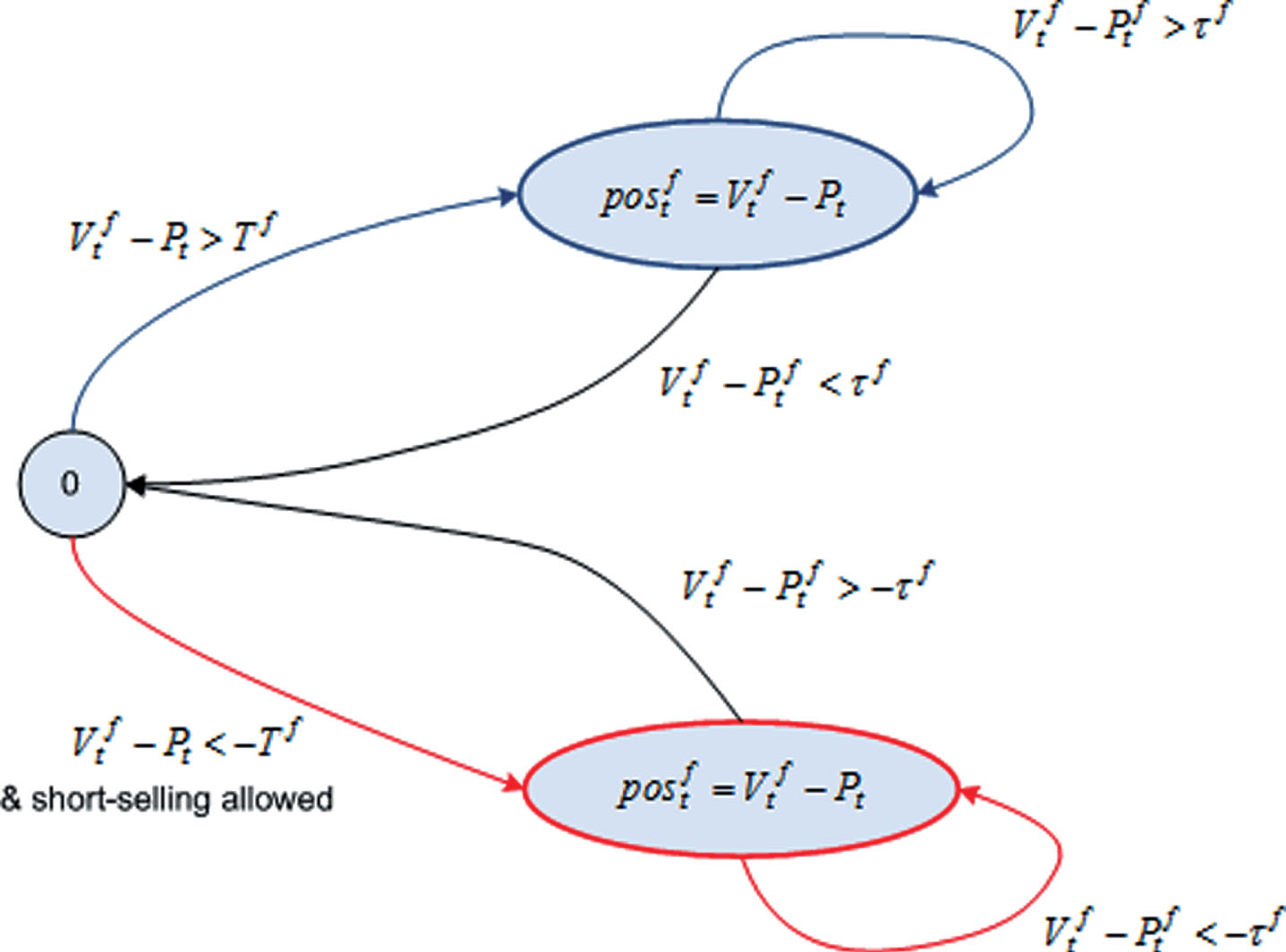

3.2.2 Technical traders (TREND)

Technical traders exploit price trends, and for that aim we have implemented two of the most common techniques in real markets (Taylor, 2005): to detect the start of a trend in prices, agents compare a short-and a long-term moving average of past prices; to detect the end of a price trend, agents rely on the technique of channel breakouts. To implement these rules, we have built on the practitioner literature, mainly on the description provided in (Kestner, 2003).

At each time step, technical investors calculate two simple moving averages (MA) of past prices: one short-term MA that responds quickly to recent price movements, and a long-term MA that responds more slowly. Let $w_{S}^{tr}$ and $w_{L}^{tr}$ be the windows used by the technical agent tr to calculate its short-and long-term moving averages, respectively. The moving averages are then given by: $MA (w_{S}^{tr})_{t} = \frac{1}{w_{S}^{tr}} \cdot \sum_{i = t - w_{S}^{tr} + 1}^{t} P_{i}$ (7) $MA (w_{L}^{tr})_{t} = \frac{1}{w_{L}^{tr}} \cdot \sum_{i = t - w_{L}^{tr} + 1}^{t} P_{i}$

When the two moving averages cross, it is the key time to buy or sell: if the short-term MA crosses the long-term MA from below, the agent interprets it as the beginning of an upward trend and opens a long position; if the short-term MA crosses the long-term MA from above, the agent interprets it as the start of a downward trend and opens a short position (if it is allowed to sell short) (Fig. 2).

Fig. 2

Illustration of the behaviour of long-and short-term moving averages.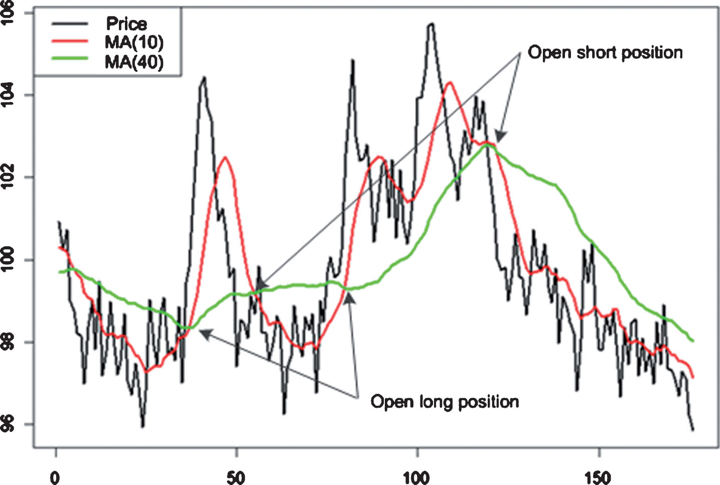

When the MA’s cross and the agent opens a position, it is proportional to the difference in slope between the two moving averages, because it is assumed that the greater this difference, the steeper the upward or downward price trend. Equations (8) and (9) specify the formula used by technical investors to calculate their position:

If $MA {(w_{S}^{tr})}_{t}$ crosses $MA {(w_{L}^{tr})}_{t}$ from below, then the agent opens a long position: ${pos}_{t}^{tr} = 25 \cdot | Δ {incl}_{t}^{tr} |$ (8)

If $MA {(w_{S}^{tr})}_{t}$ crosses $MA {(w_{L}^{tr})}_{t}$ from above, and the agent is allowed to sell short, then the agent opens a short position: ${pos}_{t}^{tr} = - 25 \cdot | Δ {incl}_{t}^{tr} |,$ (9) where

25 is a normalisation factor aimed at having the same order of magnitude in the orders from fundamentalist and technical agents.

$Δ {incl}_{t}^{tr}$ is the difference between the slope of the two MA’s:

\begin{matrix} Δ {incl}_{t}^{tr} = arctan (MA (w_{S}^{tr})_{t} - MA (w_{S}^{tr})_{t - 1}) \\ - arctan (MA {(w_{L}^{tr})}_{t} - MA (w_{L}^{tr})_{t - 1}) \end{matrix}

Technical investors keep their positions open until they think that the price trend has begun to reverse. In order to detect a trend reversal, the agents use a channel breakout rule: if the current price is the lowest in the last $w_{C}^{tr}$ days, then the technical trader interprets that the price is going down, and any long position should be liquidated; if the current price is the highest in the last $w_{C}^{tr}$ days, then the technical trader interprets that the price is going up, and any short position should be liquidated.

$\begin{matrix} If {pos}_{t - 1}^{tr} > 0 & P_{t} = = \underset{j \in [t - w_{C}^{tr} + 1, t]}{Min} {P_{j}} then {pos}_{t}^{tr} = 0 . \\ If {pos}_{t - 1}^{tr} < 0 & P_{t} = = \underset{j \in [t - w_{C}^{tr} + 1, t]}{Max} {P_{j}} then {pos}_{t}^{tr} = 0 . \end{matrix}$ (10)

Note that when drawing the minimum and the maximum of the price over a period, a channel appears, which is why the method is called “channel breakout” (Fig. 3).

Fig. 3

Illustration of the behaviour of the channel used as exit condition by the technical strategy.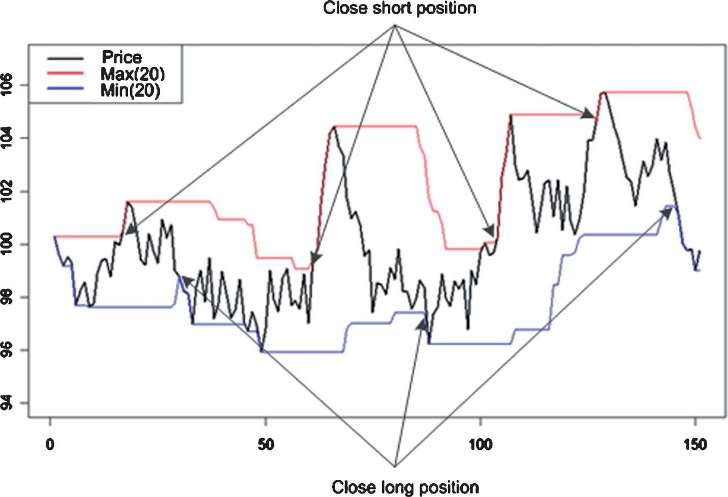

As happens with the fundamentalist investors, when a technical agent has an open position, but the channel breakout condition is not satisfied, then it simply updates its position keeping the same sign: $\begin{matrix} If {pos}_{t - 1}^{tr} > 0 then {pos}_{t}^{tr} = 25 \cdot | Δ {incl}_{t}^{tr} | \\ If {pos}_{t - 1}^{tr} < 0 then {pos}_{t}^{tr} = - 25 \cdot | Δ {incl}_{t}^{tr} | . \end{matrix}$ (11)

Technical investors are heterogeneous in the windows of the moving averages and breakout channel $\begin{matrix} w_{S}^{tr} \sim U (w_{S, min}^{tr}, w_{S, max}^{tr}), w_{L}^{tr} \sim U (w_{L, min}^{tr}, w_{L, max}^{tr}), \\ w_{C}^{tr} \sim U (w_{C, min}^{tr}, w_{C, max}^{tr}) . \end{matrix}$

Once set the new position, the agent calculates the order to be sent to the market-maker: $θ_{t}^{tr} = {pos}_{t}^{tr} - {pos}_{t - 1}^{tr} .$ (12)

Figure 4 summarises how the technical strategy works.

Fig. 4

State diagram of the technical strategy.

3.3. Parameters

Table 1 summarises the value of all the model parameters used in the results described next. When choosing these values, we have applied the following criteria:

For those parameters that are a direct adaptation of real strategy parameters, we have simply chosen realistic values. For example, the short-and long-term windows for the moving averages used by technical traders move around 10 and 40, which are the values usually employed by real technical investors (Kestner, 2003).

For those parameters not ‘observable’ in real markets (such as the liquidity λ), we have adjusted their value with the aim of obtaining reasonable price dynamics that satisfy as much as possible the stylised facts of stock markets (Cont, 2001; Taylor, 2005). For more details on how the base model has been validated and in particular for a thorough study on its capability to replicate the empirical stylised facts, see Llacay and Peffer (2018).

Table 1
Table of parameters used in the simulations

Parameter Value Parameter description

N _ticks 2000 Number of ticks of each run

λ 400 Liquidity

P ₀ 100 Initial price

σ _P 0.4 Standard deviation for random term in price formation

N _FUND 200 Number of fundamentalist traders

N _TREND 200 Number of technical traders

σ _V 0.25 Standard deviation for random term in fundamental value formation

[v_min, v_max] [– 8, 8] Boundaries of the uniform distribution that sets the difference between the fundamental value and the value perceived by each fundamentalist trader

[T_min, T_max] [2, 5] Boundaries of the uniform distribution that sets the entry thresholds of fundamentalist traders

[τ_min, τ_max] [– 0.5, 1] Boundaries of the uniform distribution that sets the exit thresholds of fundamentalist traders

$[w_{S, min}^{tr}, w_{S, max}^{tr}]$ [5, 15] Boundaries of the uniform distribution that sets the window of short-term moving average used by technical traders

$[w_{L, min}^{tr}, w_{L, max}^{tr}]$ [35, 50] Boundaries of the uniform distribution that sets the window of long-term moving average used by technical traders

$[w_{C, min}^{tr}, w_{C, max}^{tr}]$ [5, 30] Boundaries of the uniform distribution that sets the window of exit channel used by technical traders

Parameter	Value	Parameter description
N _ticks	2000	Number of ticks of each run
λ	400	Liquidity
P ₀	100	Initial price
σ _P	0.4	Standard deviation for random term in price formation
N _FUND	200	Number of fundamentalist traders
N _TREND	200	Number of technical traders
σ _V	0.25	Standard deviation for random term in fundamental value formation
[v_min, v_max]	[– 8, 8]	Boundaries of the uniform distribution that sets the difference between the fundamental value and the value perceived by each fundamentalist trader
[T_min, T_max]	[2, 5]	Boundaries of the uniform distribution that sets the entry thresholds of fundamentalist traders
[τ_min, τ_max]	[– 0.5, 1]	Boundaries of the uniform distribution that sets the exit thresholds of fundamentalist traders
$[w_{S, min}^{tr}, w_{S, max}^{tr}]$	[5, 15]	Boundaries of the uniform distribution that sets the window of short-term moving average used by technical traders
$[w_{L, min}^{tr}, w_{L, max}^{tr}]$	[35, 50]	Boundaries of the uniform distribution that sets the window of long-term moving average used by technical traders
$[w_{C, min}^{tr}, w_{C, max}^{tr}]$	[5, 30]	Boundaries of the uniform distribution that sets the window of exit channel used by technical traders

4. Results

We describe next the effects of increasing the proportion of short-sellers (parameter propSS) from 0 – no agent can have short positions – up to 1 – all agents can sell short. The rest of parameters remain constant in all the experiments to clearly identify the impact of short sales on the different tests and indicators of market efficiency 2

4.1. Statistical tests

Autocorrelation test: When running the Ljung-Box test with the return series obtained from our model, the null hypothesis is seldom accepted, what indicates that one or more autocorrelation coefficients are significantly different from zero. In fact, the return ACF tends to 0 when the lag rises, but at a slower rate than observed in real markets, and this property does not improve when the proportion of short sellers increases. Figure 5 shows the average ACF when the proportion of short sellers is 0%, 50% and 100%, and it can be seen that the first autocorrelation coefficients are significant in all the cases, which is a sign of inefficiency.

Variance ratio tests: As the variance ratio diverges from the random-walk value for some time intervals, the multiple Chow-Denning test rejects the null hypothesis in all the runs and does not capture any improvement in market efficiency when the proportion of short-sellers increases.

Runs test: Similar to the previous statistical tests, the runs test rejects the null hypothesis in almost all the runs and so one concludes that the return series are not random for any value of propSS. Again, this test does not allow to discern any enhancement of market efficiency when the number of short-selling agents is higher.

Fig. 5

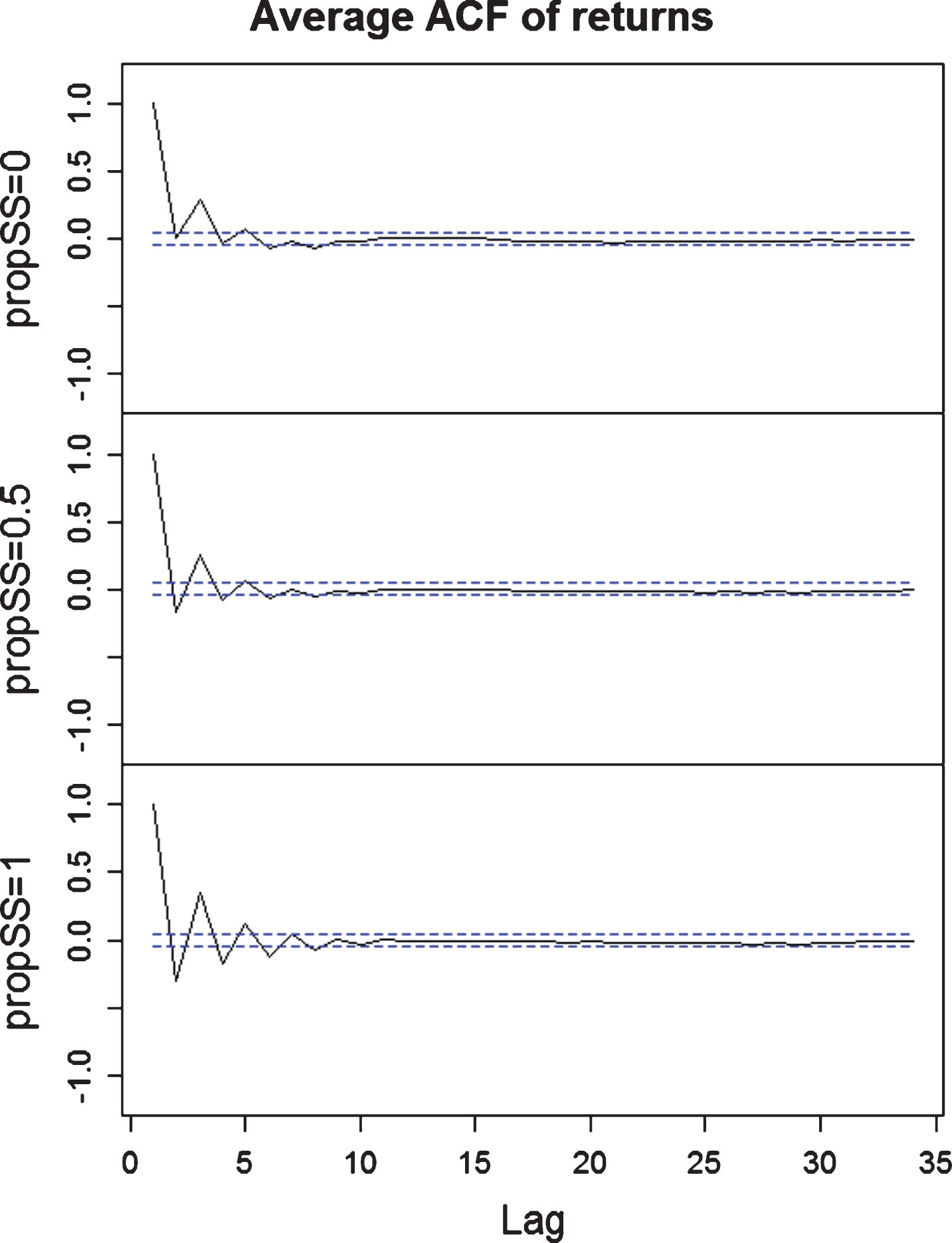
Average ACF of returns over 100 runs when the proportion of short-sellers increases (0%, 50%, and 100%).

4.2. Other indicators

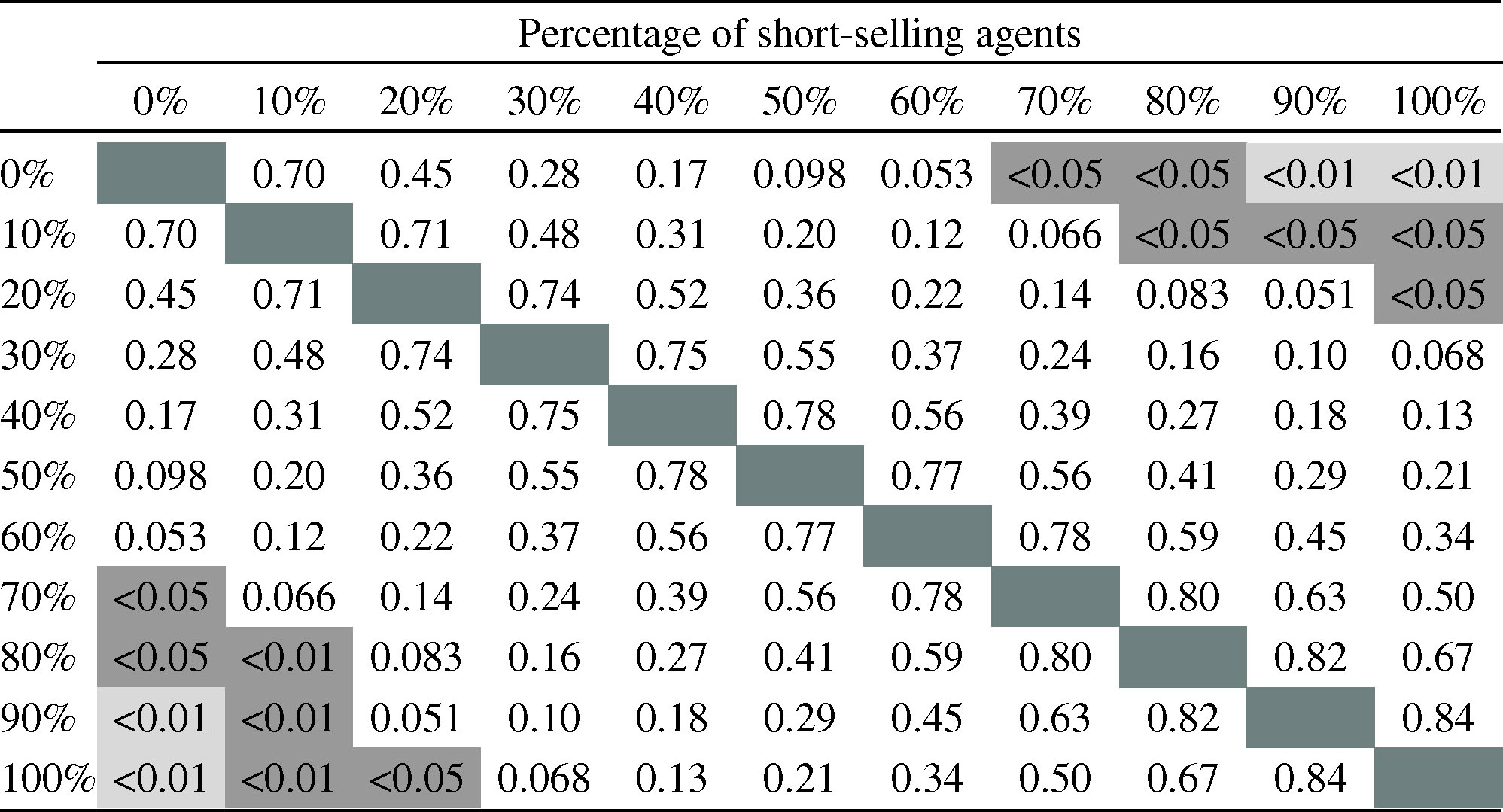
Hurst exponent: It does allow to appreciate changes between the different experiments. Figure 6 shows the evolution of the mean Hurst exponent and its range of values when the proportion of short-selling agents increases. It can be seen that the mean Hurst exponent tends to 0.5 and its range of values decreases, what indicates that short-selling increases the market efficiency, even if the market is not perfectly efficient in any experiment.

Fig. 6

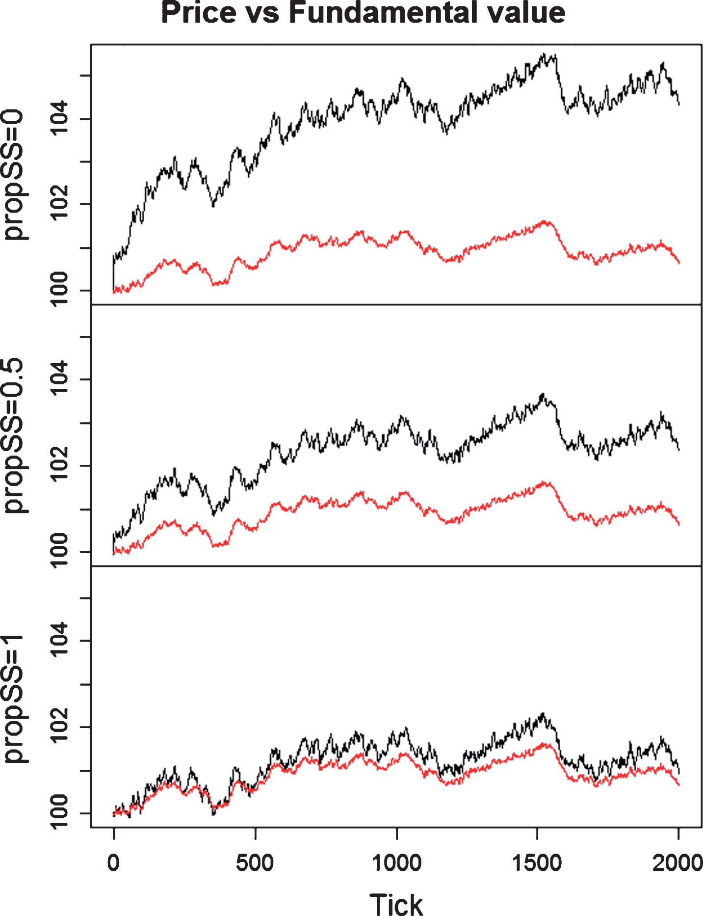
Evolution of the Hurst exponent when the proportion of short-sellers increases.

Further to the results shown in Fig. 6, we have conducted a series of t-tests to compare the Hurst exponent of the price returns under different percentages of agents being allowed to sell short. Two-sided p-values obtained from each test are shown in Table 2, where the percentages shown in row and column headers indicate the percentage of short-selling agents in the two scenarios being compared. We can observe that there is no significant difference in Hurst exponent when the percentage of agents using short-selling is similar (cells close to the diagonal of the table); however, an increase of only 20% in this percentage can produce a noticeable effect on market efficiency that leads us to reject the null hypothesis and conclude that Hurst exponent is significantly different – in Table 2 we have highlighted in yellow and orange those tests where the null hypothesis is rejected at a significance level of 0.05 and 0.01, respectively.

Table 2

P-values obtained from the series of t-tests for return Hurst exponent. The p-value reported in row x% and column y% is obtained from the t-test with null hypothesis that Hurst exponent when x% of agents are using short-selling does not differ from when y% of agents are using short-selling. Coloured cells indicate that the null hypothesis is rejected, at a significance level of 0.05 (yellow cells) or 0.01 (orange cells)

Fig. 7

Evolution of technical strategy profitability when the proportion of short-sellers increases (0%, 50%, and 100%). The time series is averaged over 100 runs.

Fig. 8

Evolution of price (in black) and fundamental value (in red) when the proportion of short sellers increases (0%, 50%, and 100%). The time series are averaged over 100 runs.

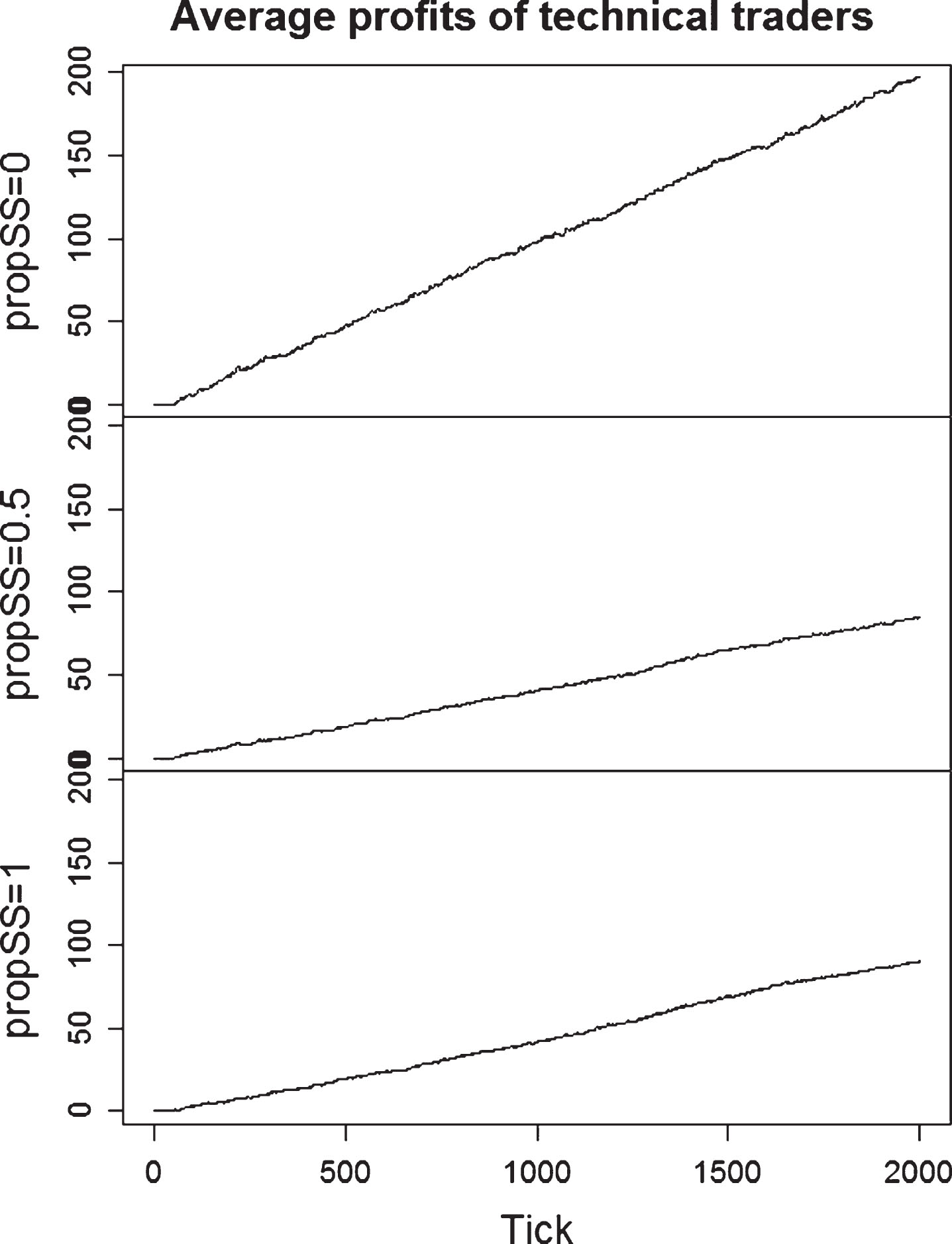
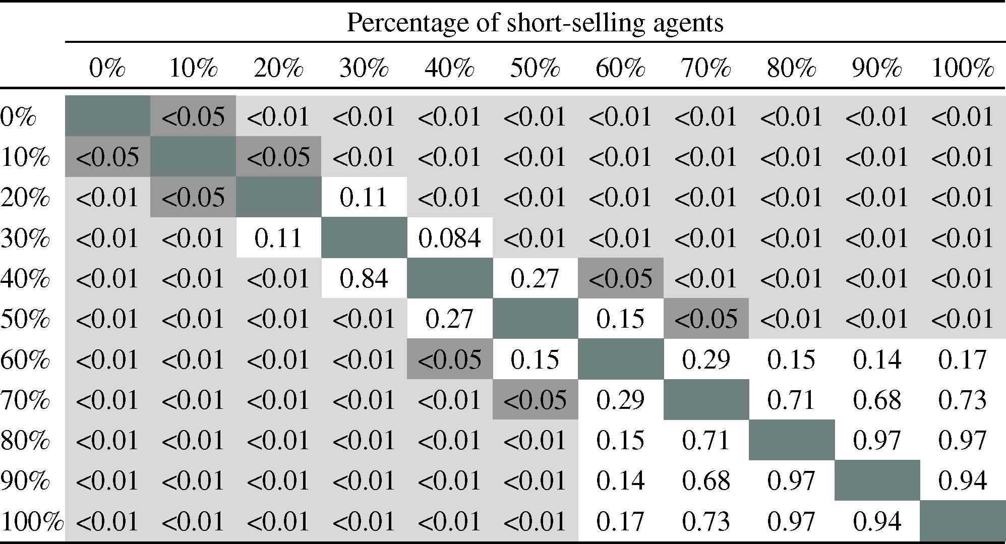
Technical strategies: The technical agents in our model are able, in average, to make profits and so the market can be concluded to be inefficient. However, when comparing the average profits of the technical traders along the different experiments, we note that their profits are higher when short-selling is not allowed, and decrease when short-sellers are introduced in the market (Fig. 7). This indicates that efficiency increases with short-selling.

As done above, we have also conducted a series of t-tests to compare the accumulated wealth of technical traders – averaged over all technical traders – under different percentages of agents using short-selling. The results, summarised in Table 3, exhibit a similar pattern: the null hypothesis gets rejected when slightly moving away from the table diagonal, meaning that a small increase in the percentage of short-sellers tends to be sufficient to produce a significant reduction in technical strategy profitability.

Table 3

P-values obtained from the series of t-tests for technical strategy profitability. The p-value reported in row x% and column y% is obtained from the t-test with null hypothesis that accumulated profits obtained by technical traders when x% of agents are using short-selling does not differ from when y% of agents are using short-selling. Coloured cells indicate that the null hypothesis is rejected, at a significance level of 0.05 (yellow cells) or 0.01 (orange cells)

Distance between price and fundamental value: When increasing the proportion of short-sellers, the price clearly approaches the fundamental value, thanks to the action of fundamental agents (Fig. 8). When agents cannot have short positions, their trading movements are limited to buying when the asset is undervalued, but they cannot take advantage of the occasions where the price lies above the fundamental value. When at least part of the fundamental population can sell short, they can exploit any asset mispricing and correct the deviations from the fundamental value process.

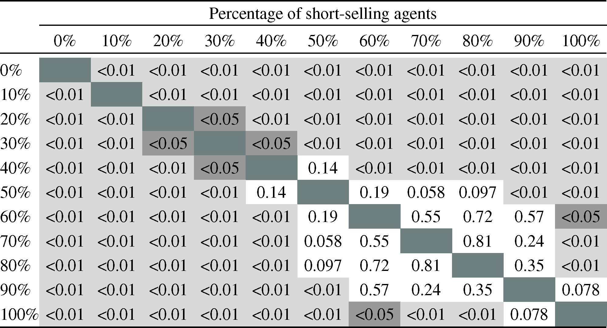
The series of t-tests conducted to compare the mean distance between the time series of price and fundamental value under different percentages of agents using short-selling, reveals that this indicator is less sensitive. The results, summarised in Table 4, show that there needs to be a noticeable increase of short-sellers in the market for the mean distance between price and fundamental value to be significantly different.

Table 4

P-values obtained from the series of t-tests for distance between price and fundamental value. The p-value reported in row x% and column y% is obtained from the t-test with null hypothesis that mean distance between the time series of price and fundamental value when x% of agents are using short-selling does not differ from when y% of agents are using short-selling. Coloured cells indicate that the null hypothesis is rejected, at a significance level of 0.05 (yellow cells) or 0.01 (orange cells)

5. Conclusions

Motivated by the recent increase of financial institutions who sell short, we have studied here the effect of short sales in stock market efficiency. We have used different tests and indicators of informational efficiency which are used in empirical studies, and applied them to the series of returns obtained from our model.

Indicators such as the Hurst exponent, the profitability of the technical strategy and the distance between the price and fundamental value indicate that short sales are beneficial to market efficiency. Although the market does not become completely efficient even when all the population can sell short, a positive improvement of its efficiency is observed. Precisely because a perfect efficiency is not reached in our model, the statistical tests (of autocorrelation, variance ratio and runs) cannot distinguish the effects of short sales and they simply indicate that the returns series is not random. By construction, it is to be expected that the price series obtained does not follow a random walk as it is determined by the actions of agents, and they do not behave randomly. Therefore, it could be envisaged that statistical tests invariably reject the null hypothesis of the random walk, and so alternative indicators such as the Hurst exponent, the profitability of the technical strategy or the distance between the price and fundamental value are more informative.

Footnotes

Appendix A: Robustness analysis

One difficulty associated to agent-based models is the calibration of the usually numerous set of parameters against real data (Thurner, 2011). In this section we analyse the robustness of the model results with respect to changes in parameter values. To this aim, we perform a sensitivity analysis using the one-factor-at-a-time methodology (ten Broeke, van Voorn and Ligtenberg, 2016), varying one parameter at a time to observe its impact on results.

We use an extreme case analysis (Taylor, 2009) where we choose an upper and lower bound for each parameter and re-run the experiments to compare the results with the base case shown in Section 4. The extreme bounds have been selected as the lowest and highest values of each parameter (1) that make sense (e.g., the long-term window used by technical traders cannot be smaller than the short-term window), and (2) for which the model is able to replicate a range of stylised facts observed in empirical markets (see Llacay and Peffer (2018)).

Next, we repeat the experiments done in section 4 for the three values of parameters: the base value, the lower bound and the upper bound. In Figs. A.1–A.11 we show the behaviour of those indicators which have turned out to be most sensible to the introduction of short sellers in the market: the Hurst exponent, the technical strategy profitability and the evolution of average price vs fundamental value. As it can be seen below, the results are robust to other parameter choices, as Figs. A.1–A.11 show the same qualitative behaviour than those shown in Section 4.

Table 5 summarises the value of all the parameters used in the robustness analyses shown in Fig. A.1–A.11. Table 5

Table of base, lower-and upper-bound parameter values used in the robustness analysis

Parameter	Base value	Lower bound	Upper bound	Parameter description
λ	400	350	450	Liquidity
σ _P	0.4	0.1	0.7	Standard deviation for random term in price formation
N _FUND	200	150	250	Number of fundamentalist traders
N _TREND	200	150	250	Number of technical traders
σ _V	0.25	0	0.5	Standard deviation for random term in fundamental value formation
[v_min, v_max]	[– 8, 8]	[– 0.5, 0.5]	[– 20, 20]	Boundaries of the uniform distribution that sets the difference between the fundamental value and the value perceived by each fundamentalist trader
[T_min, T_max]	[2, 5]	[1, 4]	[7, 10]	Boundaries of the uniform distribution that sets the entry thresholds of fundamentalist traders
[τ_min, τ_max]	[– 0.5, 1]	[– 1.5, 0]	[0.5, 2]	Boundaries of the uniform distribution that sets the exit thresholds of fundamentalist traders
$[w_{S, min}^{tr}, w_{S, max}^{tr}]$	[5, 15]	[2, 12]	[10, 20]	Boundaries of the uniform distribution that sets the window of short-term moving average used by technical traders
$[w_{L, min}^{tr}, w_{L, max}^{tr}]$	[35, 50]	[20, 35]	[60, 75]	Boundaries of the uniform distribution that sets the window of long-term moving average used by technical traders
$[w_{C, min}^{tr}, w_{C, max}^{tr}]$	[5, 30]	[1, 26]	[15, 40]	Boundaries of the uniform distribution that sets the window of exit channel used by technical traders

Acknowledgements

We would like to thank the anonymous reviewers for their insightful and constructive comments.

[1]

Code is available at https://libraries.io/github/gitwitcho/var-agent-model. Our code is implemented in Java and uses the scheduler from Repast simphony ().

[2]

The results described in this section are based on 100 runs for each value of the propSS parameter, using the same seed for random distributions for perfect comparability.

References

Anufriev, M., Tuinstra, J., 2013. The impact of short-selling constraints on financial market stability in a heterogeneous agents model. CeNDEF Working paper 13-01, University of Amsterdam.

Arthur, W., Holland, J., LeBaron, B., Palmer, R., Tayler, P., 1996. Asset pricing under endogenous expectations in an artificial stock market. SFI Working Paper 96-12-093.

Bonenkamp, U., 2010. Combining technical and fundamental trading strategies. Heidelberg: Gabler.

Bris, A., Goetzmann, W., Zhu, N., 2007. Efficiency and the bear: Short sales and markets around the world, The Journal of Finance62(3), 1029–1079.

Brunnermeier, M., Nagel, S., 2004. Hedge funds and the technology bubble, The Journal of Finance59(5), 2013–2040.

Cajueiro, D., Tabak, B., 2004. Ranking efficiency for emerging markets, Chaos, Solitons and Fractals22, 349–352.

Chaity, N., Sharmin, S., 2012. Efficiency Measures of Capital Market: A Case of Dhaka Stock Exchange, International Journal of Business and Management7(1), 102–108.

Chang, E., Lima, E., Tabak, B., 2004. Testing for predictability in emerging equity markets, Emerging Markets Review5, 295–316.

Chow, K., Denning, K., 1993. A simple multiple variance ratio test, Journal of Econometrics58, 385–401.

10.

Cont, R., 2001. Empirical properties of asset returns: Stylized facts and statistical issues, Quantitative finance1, 223–236.

11.

EC, 2008. Consultation paper on hedge funds. Working document of the Commission Services (DG Internal).

12.

Farmer, J., Joshi, S., 2002. The price dynamics of common trading strategies, Journal of Economic Behavior & Organization49, 149–171.

13.

Griffin, J., Harris, J., Shu, T., Topaloglu, S., 2011. Who drove and burst the tech bubble?The Journal of Finance76(4), 1251–1290.

14.

Hiremath, G., 2014. Indian Stock Market: An Empirical Analysis of Informational Efficiency. New Delhi: Springer.

15.

Ineichen, A., 2004. On myths, bubbles, and new paradigms in the hedge fund industry. Hedge funds: Risk and regulation. Edited by

Baums &

Cahn. Berlin: De Gruyter Rechtswissenschaften Verlags, 3–29.

16.

Johnson, N., Jefferies, P., Ming Hui, P., 2003. Financial market complexity. New York: Oxford University Press.

17.

Kerbl, S., 2010. Regulatory medicine against financial market instability: What helps and what hurts. Working paper 174, Österreichische Nationalbank.

18.

Kestner, L., 2003. Quantitative Trading Strategies: Harnessing the Power of Quantitative Techniques to Create a Winning Trading Program. New York: McGraw-Hill.

19.

King, M., Maier, P., 2009. Hedge funds and financial stability: Regulating prime brokers will mitigate systemic risks, Journal of Financial Stability5, 283–297.

20.

Llacay, B., Peffer, G., 2018. Using realistic trading strategies in an agent-based stock market model, Computation and Mathematical Organization Theory24(3), 308–350.

21.

Lo, A., MacKinlay, A., 1988. Stock market prices do not follow random walks: Evidence from a simple specification test, The Review of Financial Studies1(1), 41–66.

22.

Lux, T., Marchesi, M., 2000. Volatility clustering in financial markets: A microsimulation of interacting agents, International Journal of Theoretical and Applied Finance3(4), 675–702.

23.

Madhavan, A., 2000. Market microstructure: A survey. Marshall School of Business, Los Angeles.

24.

Malkiel, B., 1973. A random walk down Wall Street. Nueva York: Norton.

25.

Murphy, J., 1999. Technical analysis of the financial markets. Paramus: New York Institute of Finance.

26.

Nisar, S., Hanif, M., 2012. Testing Weak Form of Efficient Market Hypothesis: Empirical Evidence from South-Asia, World Applied Sciences Journal17(4), 414–427.

27.

O'Neill, B., 2011. Fundamentals of the stock market. McGraw-Hill.

28.

Quaglia, L., 2011. The ‘old’ and ‘new’ political economy of hedge funds regulation in the European Union, West European Politics34(4), 665–682.

29.

Setzu, A., Marchesi, M., 2006. The Effects of Short-Selling and Margin Trading: A Simula-tion Analysis. Presented at the 1st International Conference on Economic Sciences with Heterogeneous Interacting Agents (WEHIA 2006), Bologna, 15–17June.

30.

Spellman, J., 2009. Hedge funds: How they serve investors in U.S. and global markets. Washington: Coalition of Private Investment Companies.

31.

Taylor, S., 2005. Asset price dynamics, volatility, and prediction. Princeton: Princeton University Press.

32.

Taylor, M., 2009. What is sensitivity analysis?What is...?series, 1–8.

33.

ten Broeke, G., van Voorn, G., Ligtenberg, A., 2016. Which Sensitivity Analysis Method Should I Use for My Agent-Based Model?Journal of Artificial Societies and Social Simulation19(1).

34.

Thurner, S., 2011. Systemic financial risk: Agent based models to understand the leverage cycle on national scales and its consequences. OECD.

35.

Vitting Andersen, J., 2008. Could short selling make financial markets tumble? Available online at http://arxiv.org/abs/cond-mat/0308548v1

36.

Yagi, I., Mizuta, T., Izumi, K., 2010. A Study on the Market Impact of Short-Selling Regulation Using Artificial Markets. Advances in Practical Multi-Agent Systems. Edited by

Bai &

Fukuta. Berlin: Springer, 217–231.