Sector categorization using gradient boosted trees trained on fundamental firm data

Abstract

We examine to what extent the GICS sector categorization of equity securities may be systematically reconstructed from historical quarterly firm fundamental data using gradient boosted tree classification. Model complexity and performance tradeoffs are examined and relative feature importance is described. Potential extensions are outlined including ideas to improve feature engineering, validating internal consistency and integrating additional data sources to further improve classification accuracy.

Keywords

GICS sector gradient boosted trees fundamental data financial ratios D40 C80

1 Introduction

Major equity markets are typically comprised of thousands of stocks; however, in quantitative modeling applications one seldom considers firms as independent entities. Rather, disparate attributes of the firms such as historical equity prices and fundamental data gathered from SEC 10-Q forms are utilized to group together companies that exhibit commonalities. Seminal examples include the construction of risk factors of returns common to many equities Fama and French (1993), the identification of fundamental variables for a specific group of stocks that predict imminent bankruptcy (Altman and Naryanan, 1977), and the incorporation of non-quantitative aspects of performance such as the relationship between CEO overconfidence and associated impacts on the performance of the firm that they manage Malmendier and Tate (2005).

Equity market sectorization methods follow in a similar vein with a primary goal of representing firms as members of a hierarchical categorization. One such method widely utilized throughout the financial services industry and the academic literature is the Global Industry Classification Standard (GICS) which groups firms into eleven sectors at the coarsest level, then into twenty-four industry group categories, and finally into two further subclasses. In more detail, Standard and Poors provides a whitepaper Standard and Poors (2018) describing the main ideas behind the GICS sectorization of the United States equity market which include initially classifying a company according to its principal business activity. This is largely determined by firm revenues, earnings, and market perception; however, the final categorization decision also contains a qualitative component based upon an analyst’s view of which group the firm should become a member. We seek to understand to what extent one may systematically recover this classification mechanism from fundamental data associated with these companies by a fully systematic means. Specifically, we will pose multi-classification problems where firms’ GICS industry categorization is a target variable and several hundred features composed of fundamental variables taken from public quarterly filings documents serve as predictors.

We note that a number of authors have developed equity sector categorization methods that utilize unsupervised clustering techniques. Typically, these studies define a similarity measure between firms based on historical price data, then apply a clustering method to group similar firms. For example, in Bouchaud and Potters (2000), Harris (1991), Jung and Chang (2016), Tumminello et al. (2010), the authors demonstrate that they are able to largely reconstruct the United States equity market sectorization solely from end of day price data of constituent securities. In related literature, Hrazdil and Zhang (2012), Hrazdil et al. (2013) the authors take a different approach of considering fundamental characteristics of companies to evaluate categorization systems ultimately concluding that the GICS should be preferred over the Standard Industrial Classification (SIC). Related applications extend beyond categorization; in particular, Kumar and Ravi (2007) develop techniques for bankruptcy prediction by building models on groups of similar companies. In addition, there exists a wide body of literature aimed toward the prediction of future price returns based upon historical fundamental firm information Fama and French (1989), Kogan (2009), You and X. (2008).

Our main motivation is to understand to what extent the GICS categorization method can be reconstructed from multi-classification techniques that solely depend upon predictors constructed from quarterly firm fundamental data. In contrast to the above techniques, we consider a supervised learning approach which takes the GICS sector of each firm as a labelled target value. Specific motivations for this study include:

Develop an understanding to what extent GICS sector categorization can be systematically determined from firm fundamental data

Identify if mis-categorized stocks do not naturally fall into a GICS category which may provide portfolio managers who are constrained to trade within a given sector justification to reclassify borderline securities

Identify which features built from fundamental firm data are most relevant for GICS categorization which in turn may be fruitful inputs into subsequent predictive models

Evaluate the internal consistency of the GICS current classification system in the sense of verifying S&P’s claim that it is largely determined from fundamental equity data as well as provide analysts with an additional tool when categorizing new firms

This article is organized as follows. In Section 2, we describe the content of the dataset we consider as well as our associated feature engineering process. Next, in Section 3, we briefly summarize the gradient boosted tree classifier and comment on why it is well adapted to the multi-classification problem we are considering. Then, in Section 4, we examine the tradeoff between classifier performance and complexity and describe which features take the most prominent roles in classifier construction.

2 Dataset and feature description

First, we provide a description of our dataset acquisition, merging, and feature engineering procedures. Three distinct data sources are utilized as input into latter multiclassification models. First, we consider all numerical fields available in the Compustat North American - Daily Fundamentals Quarterly dataset accessed through Wharton Research Data Services from January 1987 to March 2018. This information is generally provided by a firm’s accounting department on a quarterly basis and was sourced from associated SEC 10-Q filings.

We next match firms on cusip values with their associated Bloomberg symbols which in turn are utilized to download their GICS sector categorization. This results in 4571 unique firms grouped into eleven mutually exclusive GICS sectors. There are 579 original fields available for each firm. We extract a subset of these variables and then construct features that will serve as inputs into subsequent multiclassification methods. We initially apply a null filter to this dataset; in particular, we remove any variable for which at least 90% of values are null, and further reduce this dataset to only consider numerical fields. After performing these filters, 110 columns remain; these are summarized in Table 5 Appendix 6. In particular, although we found fields such as firm creation date were strong predictors in certain situations, e.g. the identification of technology stocks, our aim is to determine to what extent only fundamental data may be used to create the GICS classification. From these 110 fields, we construct 40 features described in detail in Table 6. These features consist of standard financial ratios, e.g. capital intensiveness, short-term liquidity, etc., c.f. Gombola and Ketz (1983), Martikainen and Ankelo (1991). Our aim will be to build a multiclassifier on these 150 predictors and determine which are the most prominent in terms of properly grouping firms by GICS sector.

Next, we note that our dataset consists of time series of each field and feature previously described which vary in length depending upon reporting time initiation of each firm. For each such time series that consists of at least six quarters of data, we compute the mean and standard deviation of both the original and relative quarter-on-quarter changes. In addition, we also store the March 2018 value of each field as well. These comprise 750 predictors for each firm. If we are unable to compute a given value for a predictor, then we leave its value as null in the predictor matrix.

3 Gradient boosted tree multi-classification

Multiclass classification or, multi-classification for short, is the process of assigning n data points x_i into m > 2 classes where each point is labelled with a value y_i corresponding to one of these groups. There are a number of techniques that may be utilized to construct a mapping between x_i and y_i. In the context of GICS categorization, we first considered non-ensemble techniques such as decision trees, naïve Bayes, and nearest neighbor classifers. Then we extend to support vector, quadratic discriminant analysis, and neural network based classifiers. Finally, we investigated ensemble techniques including random forests, AdaBoost with decision tree weak learners, and gradient boosted decision trees. We found that gradient boosted trees provided the overall strongest performance and now discuss key themes behind these models.

Gradient boosted trees (GBT) are to decision trees as residual analysis is to multi-linear regression. In particular, one technique to account for non-linear relationships between an input and target variables is to first perform a linear regression and then examine if the associated residuals exhibit a deterministic pattern. If such a pattern exists, then it may be integrated into the original model by performing a subsequent regression on the residuals Chatterjee and Hadi (1988), and such a procedure may be iterated until the residual pattern no longer exists. In a similar manner, gradient boosting applied to decision trees is initiated by constructing a decision tree with a fixed number of leaf nodes, analyzes where classification error is greatest, and reduces these errors on the next iteration of the technique by fitting a second tree on the residuals of the first. This procedure is then iterated until a fixed number of trees is reached with the result constituting the final ensemble model. The addition of new trees is referred to as boosting and the term gradient stems from the fact that the gradient descent method is used for loss function minimization. This procedure roughly corresponds to minimizing the model error by iteratively stepping in the direction of the gradient of the model objective function. The learning rate of the model is a scale factor on this step size. In summary, there are three model parameters that need to be tuned for gradient boosted trees: the number of leaf nodes of each tree, the total number of trees in the ensemble, and the learning rate. We refer the reader to Ke (2017) for a more detailed technical description of this technique.

The nature of iteratively fitting residuals makes GBT models prone to overfitting. If one fails to establish a proper training and testing framework, it is highly likely that this model will overfit residual error structures in the training set; this will result in a low bias but high variance model that will not perform well on the holdout test dataset. With this in mind, for each model considered below, we divide available data into a 20% test hold-out portion used only for final performance evaluation as well as an 80% training dataset. In addition, we found after extensive cross-validation studies that setting the learning rate to 1/20 resulted in the swiftest convergence and most accurate overall models on average. Thus it remains to tune the number of trees and leaf nodes which we consider further below.

To be more precise, GBT models are initialized with a single decision tree. In the example considered in this work, such a tree is constructed by selecting a feature, thresholding on a value of this feature which in turn determines a binary split in the tree that branches to its subsequent level. This process is repeated until a fixed number of leaf nodes is achieved. The threshold value and feature node is determined at each level by maximizing the information gain criteria of the split. More precisely, define the Shannon entropy on a collection of data points X by $H (X) = - \sum_{k = 1}^{m} p (k) ln p (k),$ (1) where here p (k) denotes the ratio of total datapoints belonging to the k-th group. Note that the entropy is maximized in the event that the p (k) are identical and minimized in the case where it is identically zero when all data resides in a single class. The aim of decision tree construction is to maximize the difference in entropy from one level of the tree to the next. In particular, we note that if a feature and threshold are set, then the dataset X is split into two subsets X₁ ∪ X₂ = X. The information gain is defined to be the difference in entropy prior to and the mean entropy after the split, namely

$\begin{matrix} IG (X, X_{1}, X_{2}) \\ = H (X) - \frac{| X_{1} |}{| X |} H (X_{1}) + \frac{| X_{2} |}{| X |} H (X_{2}) . \end{matrix}$ (2) Information gain is iteratively maximized until a stopping criteria of reaching a fixed number of leaf nodes is satisfied. Next, boosting consists of constructing an ensemble F (x) of individual tree models f_k (x) whose mode we denote by F (x). The main aim is to minimize total mis-classification error $\hat{F} = \underset{F}{argmin} \sum_{i = 1}^{n} l (y_{i}, F (x_{i})),$ (3) where here the loss function l (y, x) is binary and counts if a datapoint is misclassified, with zero value if the classification is correct. This minimization is achieved in the setting of gradient boosting by approximating the objective function by a quadratic

$\begin{matrix} \hat{F} & = \sum_{i = 1}^{n} l (y_{i} + f_{k} (x_{i})) \\ \approx \sum_{i = 1}^{n} l_{i} (y_{i}) + g_{i} f_{m} (x_{i}) + \frac{h_{i}}{2} f_{m} (x_{i})^{2}, \end{matrix}$ (4) where here g_i = ∂l_i (y_i)/∂y_i and $h_{i} = \partial^{2} l_{i} (y_{i}) / \partial y_{i}^{2}$ . Variations in gradient boosted trees differ based upon how they estimate the gradient g_i and Hessian h_i. This ensemble model is constructed by iteratively fitting and updating the residuals of this fit in the case of gradient boosted trees. Namely, one first fits a decision tree, then uses it to make predictions of the categories of the x_i, which we denote by ${\hat{y}}_{i}$ . Next, we compute the residuals of the first iteration $e_{1} = y - {\hat{y}}_{1}$ , and then fit a second tree using e₁ as a target and use it to predict the residuals ${\hat{e}}_{1}$ . This in turn is used to update our original predictions to ${\hat{y}}_{2} = {\hat{e}}_{1} + {\hat{y}}_{1}$ , and the process is then repeated a fixed number of times. We utilize the LightGBM gradient boosted tree algorithm described in Ke (2017) to which we refer for a more detailed discussion.

4 Numerical Studies and GBT Classification Performance

We now perform numerical studies aimed toward the evaluation of the performance of GBT models’ ability to classify a firm’s GICS sector from fundamental data. First, we examine the sector classification accuracy of GBT models as a function of the total number of trees and leaf nodes, i.e. we perform hyperparameter optimization on the two central parameters that define a GBT model. In addition, we consider how the model log-loss function’s value is reduced as a function of the number of iterations during the model training process in the example of the model with overall greatest classification accuracy.

We first consider the accuracy of the GBT over a range of values for the total number of leaf nodes and iterations considered during the training process. One increases model complexity when considering increased numbers of leaf nodes and although it is always possible to reduce error on the training set, we find that after extending beyond five leaf node trees that we experience overfitting and the model performance on the test set degrades independent of the number of iterations of the algorithm. Specific classification accuracy results are presented in Table 1 where we consider GBTs between two and sixteen leaf nodes and 25 to 200 iterations.

Table 1
Average GICS sector classification accuracy for GBT models of varying numbers of residual fit iterations (Itr) and maximum leaf nodes (Nodes) trained on fundamental data from 1/1991 to 1/2018

Itr/Nodes 2 3 4 5 8 10 12 16

25 47.4 53.3 54.9 56.2 57.0 57.6 56.5 57.1

50 51.5 56.3 58.0 59.5 59.6 58.8 58.1 59.0

75 54.2 59.4 59.7 60.3 59.9 60.8 58.3 60.3

100 56.0 60.5 60.3 61.5 60.6 60.5 59.7 60.6

125 58.2 60.8 61.0 62.1 62.1 61.5 60.6 60.9

150 58.3 61.7 61.4 62.8 61.8 61.8 60.8 60.9

175 58.6 61.8 62.2 62.8 62.1 61.8 60.8 60.9

200 59.0 62.1 62.1 63.1 62.1 61.8 60.8 60.9

Itr/Nodes	2	3	4	5	8	10	12	16
25	47.4	53.3	54.9	56.2	57.0	57.6	56.5	57.1
50	51.5	56.3	58.0	59.5	59.6	58.8	58.1	59.0
75	54.2	59.4	59.7	60.3	59.9	60.8	58.3	60.3
100	56.0	60.5	60.3	61.5	60.6	60.5	59.7	60.6
125	58.2	60.8	61.0	62.1	62.1	61.5	60.6	60.9
150	58.3	61.7	61.4	62.8	61.8	61.8	60.8	60.9
175	58.6	61.8	62.2	62.8	62.1	61.8	60.8	60.9
200	59.0	62.1	62.1	63.1	62.1	61.8	60.8	60.9

We note that we fixed a maximum of 200 iterations as in an extended study we found that no substantive accuracy improvements existed beyond 200 iterations independent of the number of leaf nodes. Test set accuracy was strongest with the five leave two-hundred iteration GBT. We next examine how the model loss function error is reduced as a function of the number of residual fit iterations in Fig. 1.

Fig. 1

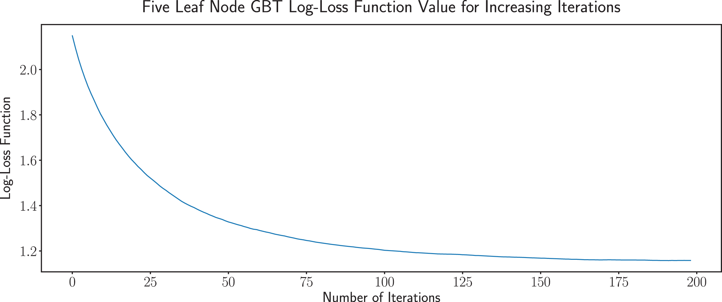
Plot of the log-loss function for a 5-leaf node GBT with 63.1% accuracy up to 200 iterations.

Note that we have steep decline in the log-loss error over the first fifty iterations which asymptotes to a value of approximately 1.2 as one approaches 200 iterations. This behavior is consistent with what we have observed when the number of leaf nodes varies differs from five as well.

We next consider the confusion matrix of the five leaf two-hundred iteration classifier in Figure 2. The confusion matrix depicts the percentage of firms that were classified into the sectors labelled on the columns of the graphic given that their true GICS sector value is on the row of each graphic.

Fig. 2

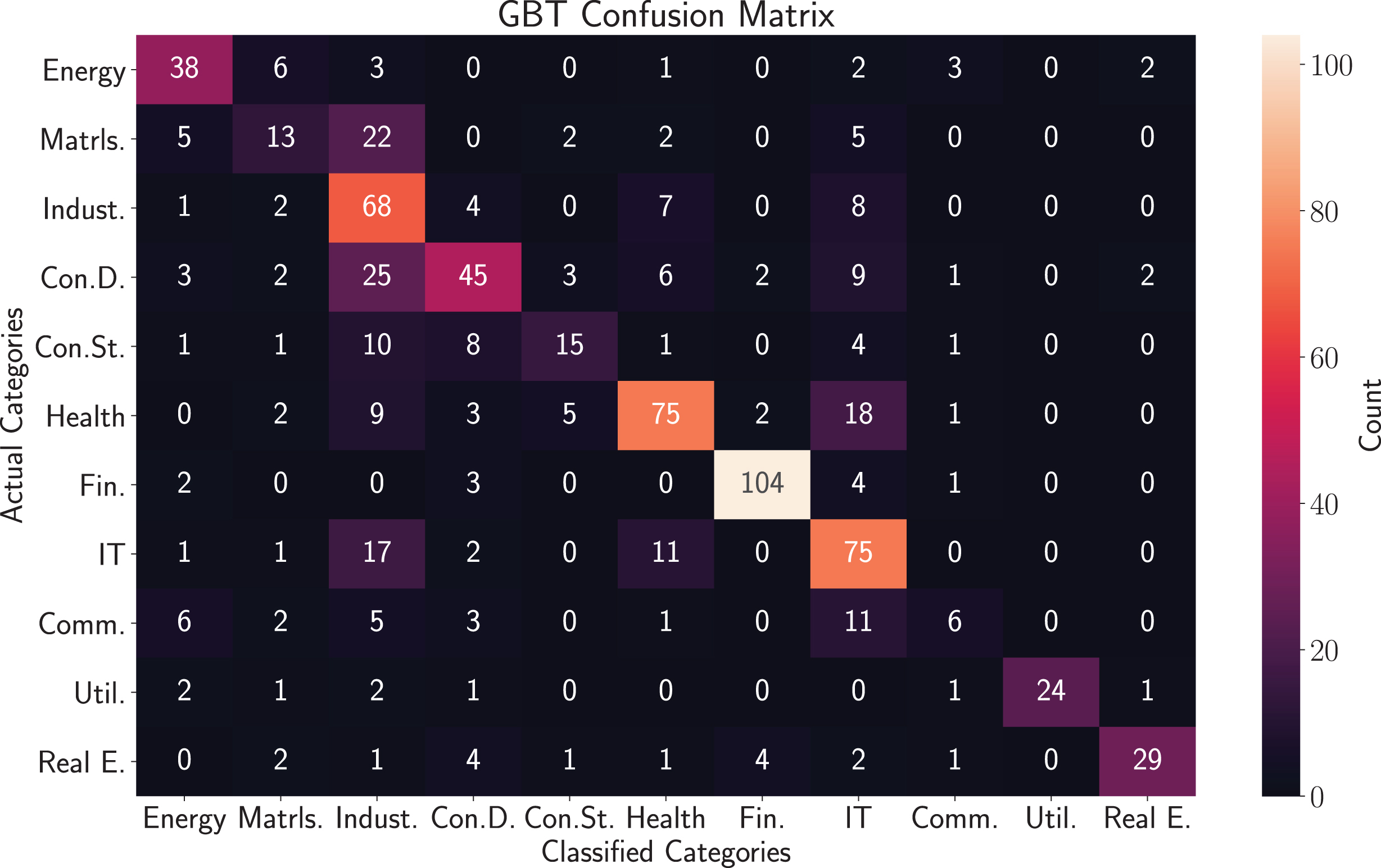
Confusion matrix of the five maximum leaf node and two-hundred iteration GBT model. Values correspond to what percentage of firms whose true GICS sector is identified by the row label were classified into each sector. For example, 11% of firms with GICS sector Energy were classified as Materials firms.

Of the 780 firms in the test set, we note that 162 were classified as Industrial, 138 Info. Tech, 112 Financials, 105 Health Care, 73 Con. Discretionary, 59 Energy, 34 Real Estate, 32 Materials, 26 Con. Staples, 24 Utilities, and 15 Comm. Services. Of the sector categories into which more than one-hundred firms were classified into, the classifier performed well with a mean accuracy of 74%. It performed poorly in the Materials, Consumer Staples, and Communication sectors. In particular, 39% of firms that were actually Materials firms were classified as Industrial firms which indicates that there may be a degree of ambiguity between these sectors. Similarly, 41% of Communication Services firms were classified as Information Technology firms. We note that such classification error is most likely due to the small sample size of communications firms considered.

Next, we consider the relative important of how different features contribute to the GBT model. In particular, we enumerate all node variables used to split the tree in this ensemble model and report their associated percentages in Table 2. Note that the mean of the receivables inventory ratio is the most prominent feature in the model. Second, the cost of goods sold over inventory ratio and research expense and current debt to total debt ratio occur with roughly half the frequency of the leading feature.

Table 2

Feature importance in the sense of enumerating all variables used to split each tree in the 5 leaf node 200 iteration GBT model and determining the frequency of occurrence of each variable; here values are represented as percentages

Feature	Importance	Feature	Importance
rs_f_mn	1	cftd_f_mn	0.302
csq_f_mn	0.559	cdtd_f_chg_std	0.297
xrdq_mn	0.516	invtq_mn	0.289
cdtd_f_mn	0.492	cshfdq_chg_mn	0.285
xrdq_std	0.378	recchq_std	0.285
aa_f_mn	0.368	sw_f_mn	0.283
cta_f_mn	0.338	ibmiiq_mn	0.281
dviq_mn	0.335	cstkq_mn	0.279
capsq_std	0.332	wta_f_mn	0.276
invchq_std	0.326

We finally compare several multi-classification models which we considered in addition to the GBT in terms of their overall accuracy, balanced accuracy and log loss function. Here, the balanced accuracy is defined to be the average recall taken over each class which is intended to normalize the notion of accuracy for imbalanced datasets.

In addition, note that the accuracy of the LGBT and random forest models are comparable. Also, the ExtraTrees classifier had similar accuracy performance as well. These results suggest that tree-based models are best suited for the GICCs sector classification problem.

In the case of the gradient boosted tree model, we compute additional metrics at the level of the individual categories and average metrics over categories which represent the full classifier. Specifically, define the micro and macro precision and micro and macro recall to be

$\begin{matrix} mP = \frac{\sum_{i} {TP}_{i}}{\sum_{i} {TP}_{i} + \sum_{i} {FP}_{i}}, mR = \frac{\sum_{i} {TP}_{i}}{\sum_{i} {TP}_{i} + \sum_{i} {FN}_{i}}, \\ MP = \frac{1}{n} \sum_{i} P_{i}, MR = \frac{1}{n} \sum_{i} R_{i} . \end{matrix}$ (5)

where here we here TP denotes the true positive count, FP the false positive count, FN the false negative count, P the precision, and R the recall. In the example of the five leaf node two hundred iteration gradient boosted tree classifier, we calculate mR = mP = 0.631, MR = 0.579, MP = 0.646. Next, we compute the precision, recall, and F1 score across the eleven GICS sector categories. The results are summarized in Table 4 below where here we refer to Standard and Poors (2018) for a dictionary between GICS sector code and category labels.

Table 3

We compare GICS sector multi-classifier performance across eight models in terms of overall Accuracy, Balanced Accuracy, and the value of the model log-loss function

Model	Accuracy	Balanced Accuracy	LogLoss
LGBT	0.631	0.579	1.158
Random Forest	0.621	0.559	1.182
ExtraTrees Classifier	0.607	0.532	1.231
Smooth Ridit Transform SGD	0.604	0.545	1.285
Standardize SGD	0.502	0.428	1.562
Decision Tree	0.442	0.364	1.846
Neural Net. Classifier (256 hidden units)	0.486	0.441	1.954

Table 4

Individual GICS Sector Category Precision and Recall Scores

GICS Sector Code	10	15	20	25	30	35	40	45	50	55	60
Precision	0.64	0.41	0.42	0.62	0.58	0.71	0.93	0.54	0.4	0.1	0.85
Recall	0.68	0.27	0.76	0.46	0.37	0.65	0.91	0.7	0.18	0.75	0.64
F1 Score	0.67	0.32	0.54	0.52	0.45	0.68	0.92	0.61	0.24	0.86	0.73

5 Conclusions

In summary, we have constructed a dataset merging fundamental firm data obtained from Compustat together with GICS sector and industry group information. We then show that GICS sector categorization can be largely reconstructed using gradient boosted tree multiclassifers. We finally summarized the confusion matrix and present the most prominent features in the later case.

There are a number of extensions and further studies to consider. First, GBTs are able to capture the nuanced structure of the GICS sector and industry group classification systems. We would like to consider further feature engineering beyond the financial ratios and summary statistics already considered with the intent of further reducing model complexity through stronger predictors. In addition, we would like to examine pruning steps to reduce the complexity of the trees that compose the GBT models. It would also be of interest to explore ensemble models consisting of simple GBTs together with other distinct multiclassifers such as support vector and quadratic discriminant analysis to further explore the aggregate classifer accuracy/complexity tradeoff. On a separate note, it would be of interest to build upon the work of Hrazdil et al. (2013) to compare GICS to other industry classification systems such as SIC, IDB, TRBC, Factset’s RBICS, Morningstar’s MGECS, and Bloomberg’s BICS, to assess the internal consistency of each method. Finally, the features that are most important for distinguishing a firm’s sector are likely to also be useful for subsequent predictive models that we will consider for future security return and volatility prediction.

Source Code

A public repository hosted on github.com which contains the source code for main classifier examined in this article is available at: https://github.com/steve98654/gicsproj/

The authors would like to acknowledge Zachary David whose thoughts greatly improved the content and testing framework of this article.

Footnotes

Appendix A. Field Descriptions

We provide a list of column name acronyms for the Compustat fields considered in the above classification studies in Table 5 and refer to the User’s Guide Poor’s (2002) for further detail and definitions.

In Table 6, we define features considered in the above in terms of related Compustat fields.

Acknowledgments

The authors would like to acknowledge Zachary David whose thoughts greatly improved the content and testing framework of this article. S. Taylor was partially sponsored by the Grant Agency of the Czech Republic, grant 19-28231X.

References

Altman

E.I.

, Naryanan

, 1977. Zeta analysis: A new model to identify bankruptcy risk of corporations, Journal of Banking and Finance1(1), 29–54.

Bouchaud

J.P.

, Potters

, 2000. From Statistical Physics to Risk Management. Cambridge University Press.

Chatterjee

, Hadi

, 1988. Sensitivity Analysis in Linear Regression. John Wiley and Sons.

Fama

E.F.

, French

K.R.

, 1989. Business conditions and expected returns on stocks and bonds, Journal of Financial Economics25(1), 23–49.

Fama

E.F.

, French

K.R.

, 1993. Common risk factors in the returns on stocks and bonds. Journal of Financial Economics33, 3–56.

Gombola

, Ketz

J.E.

, 1983. A note on cash flow and classification patterns of financial ratios, The Accounting Review58(1), 105–114.

Harris

, 1991. Stock price clustering and discreteness, The Review of Financial Studies4(3), 389–415.

Hrazdil

, Zhang

, 2012. The importance of industry classification in estimating concentration ratios, Economics Letters114(2), 224–227.

Hrazdil

, Trottier

, Zhang

, 2013. A comparison of industry classification schemes: A large sample study, Economics Letters118(1), 77–80.

10.

Jung

S.S.

, Chang

, 2016. Clustering stocks using partial correlation coefficients, Physica A: Statistical Mechanics and its Applications462(15), 410–420.

11.

, 2017. A highly efficient gradient boosting decision tree. 31st Conference on Neural Information Processing Systems (NIPS 2017).

12.

Kogan

, 2009. Predicting risk from financial reports with regression. Proceeding NAACL ’09 Proceedings of Human Language Technologies, pages 272–280.

13.

Kumar

P.R.

, Ravi

, 2007. Bankruptcy prediction in banks and firms via statistical and intelligent techniques a review. European Journal of Operational Research180(1), 1–28.

14.

Malmendier

, Tate

, 2005. Ceo overconfidence and corporate investment. The Journal of Finance60(6), 2661–2700.

15.

Martikainen

, Ankelo

, 1991. On the instability of financial patterns of failed forms and the predictability of corporate failure, Economic Letters35, 209–214.

16.

Standard & Poor’s. Compustat (Global) Data Guide. McGraw-Hill Companies, 2002.

17.

Standard and Poors. 2018. Global Industry Classification Standard (GICS) Methdology. Standard and Poors Down Jones Indicies.

18.

Tumminello

, Lillio

, Mantegna

, 2010. Correlation, hierarchies, and networks in financial markets, Journal of Economic Behavior and Organization75, 40–58.

19.

You

, Zhang

, 2008. Financial reporting complexity and investor underreaction to 10-k information, Review of Accounting Studies14(4), 559–586.