
Abstract
We describe a systematic approach called reframing, defined as the process of preparing a machine learning model (e.g., a classifier) to perform well over a range of operating contexts. One way to achieve this is by constructing a versatile model, which is not fitted to a particular context, and thus enables model reuse. We formally characterise reframing in terms of a taxonomy of context changes that may be encountered and distinguish it from model retraining and revision. We then identify three main kinds of reframing: input reframing, output reframing and structural reframing. We proceed by reviewing areas and problems where some notion of reframing has already been developed and shown useful, if under different names: re-optimising, adapting, tuning, thresholding, etc. This exploration of the landscape of reframing allows us to identify opportunities where reframing might be possible and useful. Finally, we describe related approaches in terms of the problems they address or the kind of solutions they obtain. The paper closes with a re-interpretation of the model development and deployment process with the use of reframing.
Introduction
Reuse of learnt knowledge is of critical importance in the majority of knowledge-intensive application areas, particularly because the operating context can be expected to vary from training to deployment. In machine learning this has been most commonly studied in relation to variations in class and cost skew in classification. While one crisp classifier outputting class labels may be sufficient and highly specialised for one particular operating context (e.g., the positive class being ten times more likely than the negative class), it may not perform well for significantly different operating contexts (e.g., balanced classes). Instead of training several specialised models for each particular operating context, it is more cost-effective to learn one general, versatile model, such as a scoring classifier outputting scores or probabilities, which can be adapted to several contexts through an appropriate procedure, such as the choice of a decision threshold.
In this paper we develop the hypothesis that this successful but narrow approach can be generalised to many other problems and areas in machine learning, where models are required to be more general and adaptable to changes in the data distribution, data representation, associated costs, noise, reliability, background knowledge, etc. This naturally leads to a perspective in which models are not continuously retrained and re-assessed every time a change happens, but rather kept, enriched and validated in a long-term ‘model life-cycle’. We define this generalised approach, which we call reframing, as the process of preparing and devising the model deployment procedure to perform well over a range of operating contexts beyond the specific context in which the model was trained. Figure 1 provides an illustration of this process, in which the notion of a versatile model, able to generalise over a range of contexts, is key.
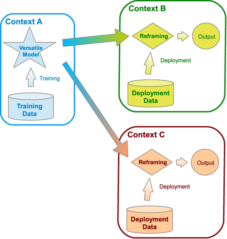
A general, versatile model is learnt in context A so that it can be reframed to operate in many other contexts (e.g., B and C) without retraining it repeatedly.
Many other recent machine learning approaches have addressed the need to cope with context changes. Areas such as domain adaptation, transfer learning, transportability, meta-learning, cost-sensitive learning, incremental and online learning, among others, have proposed new techniques and methods. However, only some of these approaches really perform model reuse, i.e., the same model being applied systematically for changing contexts. Generally, in these areas the context change is analysed when it happens, rather than being anticipated. Reframing, in contrast, formalises the expected context changes before any learning takes place, parametrises the space of contexts, analyses its distribution and creates models that can systematically deal with that distribution of context changes. This can only be achieved by a versatile model, which is reframed using the particular context information for each deployment situation, and not retrained or revised whenever the operating contexts change. Rather than being an umbrella term for the above-mentioned related areas, reframing is a distinctive way of addressing context changes by anticipating them from the outset.
The rest of the paper is organised as follows. In Section 2 we define and discuss the central notions of context and context change as they manifest themselves in machine learning. Section 3 discusses the three main alternatives for adapting to context: retraining, revising and reframing. The latter is further elaborated in Section 4, where we distinguish the three main kinds of reframing. Section 5 considers the important question of context-aware performance evaluation and visualisation. Section 6 reviews existing approaches that are related to reframing and the general goal of adapting to multiple contexts. Section 7 concludes.
In this section we provide a definition of context, a taxonomy of context changes and a discussion of issues relating to context characterisation.
A parametrised context θ is a tuple of one or more parameter values, discrete or numerical, that represent or summarise the kind of variable information, extrinsic to the data, that affects the data distribution, data representation, data quality, the utility function, or the task itself.
For instance,
Next we present a taxonomy of context changes (summarised and exemplified in Table 1) that are commonly observed in machine learning applications. Although not intended to be exhaustive or mutually exclusive, this taxonomy can help to bring together previous work developed in different but related areas.
Taxonomy of context change types and examples of their parametrisation
Taxonomy of context change types and examples of their parametrisation
Distribution shift. The most obvious type of context change is given by a change in the data distribution. One common way of looking at a change in the data is known as data shift [49,53]. Data shift is usually classified into covariate shift, prior probability shift and concept drift, but more thorough classifications have been developed (see, e.g., [49]).
Costs. This context category includes, for instance, changes in misclassification costs or changes in tolerance levels and asymmetric costs for regression models [8,32,36]. Often data shift and cost context changes are closely related. For instance, in ROC analysis, class distribution and cost proportions can be combined into the notion of skew [25].
Data quality. The quality of the data can also change from context to context, due to a variety of domain-dependent reasons (e.g., faults, random fluctuations, low reliability of attributes, …). For instance, some applications may suffer changes in the noise level (both in input and output) in such a way that models can be adapted to produce more reliable outputs [28].
Representation change. This category is observed when the attribute representation or their meaning changes from context to context. For instance, some attributes may be merged, or the granularity of the data may change [46] (e.g., a model was built for forecasting sales at city-level but will now need to be adapted to country-level).
Task change. A more radical context change is when the task itself changes. For instance, in a classification task new classes can appear in the deployment data, without having been observed in the training data [56]. As another example, a regression task may become a classification task due to new objectives. In this case, one can build a classifier for the new context by applying a cutoff to the original regressor’s outputs [34].
Often the deployment context is not explicitly given and needs to be (partly) inferred. In general, we need an estimate of the context
For instance, in binary classification we may be given a cost matrix, from where we get a single parameter c, representing the cost proportion. But we may additionally need to know the class proportion during application time. Since we can infer this proportion from a few labelled examples observed in the deployment context, Γ is a very simple procedure in this case, which requires neither the trained model m nor the original context c.
Alternatively, suppose we have learnt a model m with a training dataset that has a ratio c of positives against negatives. In deployment, we may have a small labelled dataset where we infer that the ratio is
As an example where the model itself can be helpful to infer the context, consider the input data shift, also known as covariate shift. One way to confirm a hypothetical shift is if it improves a model’s performance on some deployment data [3].
It is important to highlight that reframing, as we will see in the following section, does not require a threshold above which a context change triggers some kind of action (e.g., a revision of the model). On the contrary, reframing works with the parametrised context information, independently of whether there is a slight or a dramatic change with respect to the most recent model deployment. In other words, reframing is not triggered when there is a significant context change, but rather applied systematically for any context (changed or not).
Finally, the description of a context can be accompanied by a distribution across
Context-aware approaches for machine learning
In this section we discuss different approaches to deal with the variety of contexts described above. We discuss the choice between retraining, revision and reframing, and the notion of a versatile model. The section includes examples of these different approaches and ends with hybrid cases crossing the boundaries of one single approach.
We assume that in each context there is a task (possibly different for each context) that consists in providing certain estimates given some input data. We denote the type of input as
A context-blind approach would be to learn a model
Perhaps the simplest kind of context-aware setting arises when the context is encoded as a feature value. This allows a decision tree, for example, to split on the context feature and to construct context-specific submodels below that split. For this to work we need sufficient training data covering a wide range of training contexts, which may be prohibitive in some situations. Whether model reuse takes place at all depends on where the context feature is used: the lower this is in the tree, the more of the model is shared across contexts. Conversely, if the context is used at the root we obtain a set of unrelated context-specific models.
The context-as-a-feature approach may be blind to the global influence of the context on other features or the data distribution. Also, machine learning techniques may be unable to process that information effectively. For instance, it is unusual to treat cost as an extra input feature. Instead, we will analyse below three approaches where context is considered as key information that affects the whole problem.
Retraining
There may be no need to create all context-specific models at once, as in the case of decision trees above using the context as a feature. Rather, we could create them in an on-demand fashion. That is, each time we need to adapt to a new context we collect sufficient training data for that context and build a new context-specific model. We refer to this approach as retraining, and it provides a second baseline to compare against. There are two different subtypes:
In both cases, there can be knowledge reuse, such as the use of the optimal parameters or some parts of the original models from some previous training situations.
Revision
Retraining a model again and again whenever something changes is often inefficient, especially if the context change is small and the retrained model is similar to the original one. A common alternative to retraining is model revision, where parts of the model are patched or extended according to a new context [14,54].
Model revision is particularly appropriate when there is a concept drift [29], but it can deal with any of the other types of context changes discussed in the previous section. It is particularly natural as a result of incremental learning [39] or lifelong learning [60], but can also be used in other cases of domain adaptation when there is a mapping between two different domains [48].
A key issue in model revision is the detection of novelty or inconsistency of the new data with respect to the existing model, as in the area of theory revision [54]. In this case, the revision of a theory is triggered when the semantics of the model are affected, as it does not fully accommodate the new evidence. This can be extended to context changes, provided we can determine when the context has changed significantly to deserve a revision process.
Whether revision is a viable option depends on the model class: rules and linear models are easier to revise than neural networks and support vector machines.
Reframing and versatile models
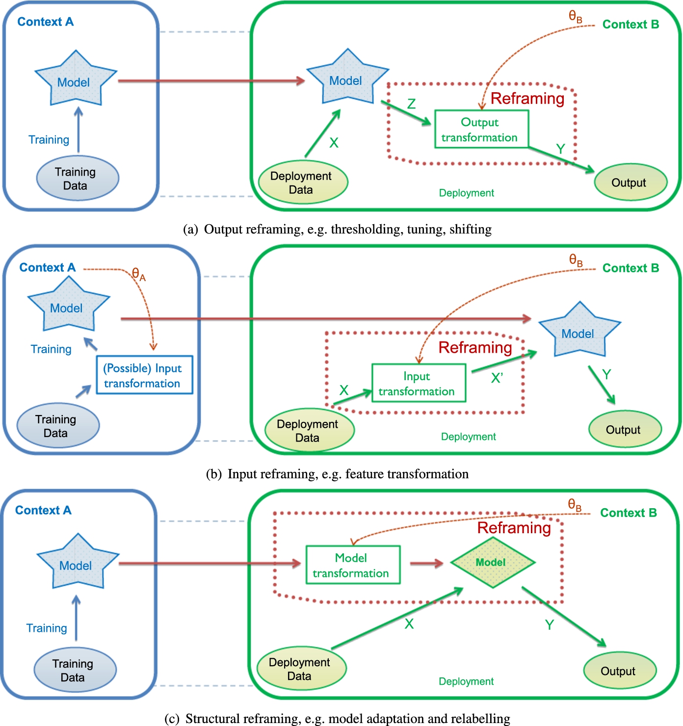
Reframing is a context-aware approach that reuses a model m built in the training context by subjecting it to a reframing procedure that takes into account the particular deployment context. As elaborated in the next section, we distinguish three different kinds of reframing (which can be combined):
Which type of reframing should be used depends on what aspects of the model are reusable in other contexts. If these aspects are known in advance, then it is possible to design a training procedure which results in a versatile model: a model capturing the reusable knowledge. Thus, where a conventional, non-versatile model captures only such information as is necessary to deal with test instances from the same context, a versatile model captures additional information that, in combination with reframing, allows it to deal with test instances from a larger range of contexts.
Note that a versatile model might have a different data signature for input and output than the original task signatures
In a way, most decision rules and feature construction procedures can be seen as reframing processes, provided that the context is used in the transformations. In supervised tasks, generative models estimating
Versatile models can be composed of submodels, which may be combined in different ways depending on the context.
Choosing the best approach: Examples
Given the alternatives described above, which one is best? There is no general answer, as this may depend on the problem and the kind of context. Also, we can use more than one approach or a hybrid. Nevertheless, we can give some guidelines.
Retraining on the training data is very general and popular, because it is easy and applicable to any model class, but there are many cases where it is not applicable. For instance, the training data may have been lost or may not exist (e.g., models have been created or modified by human experts) or may be prohibitively large (if deployment must work in restricted hardware), or the computational constraints do not allow retraining for each deployment context separately. Retraining on the deployment data can work well if there is an abundance of deployment data, but often the deployment data are limited, unsupervised or simply do not exist. For instance, in open set recognition [56] not all classes are present in the training data and the model has to be versatile enough to cover for classes that will appear in the deployment dataset.
Revision is usually a complex process that is highly dependent on the technique that one is using. Of course, there are cases between retraining and revision where it is difficult to draw a line, as when all parameters of a Bayesian model are acquired (and not only adjusted) on new data. Model revision changes the semantics of the model, and this does not correspond well with some types of contexts. For instance, if we have a cost change or a task representation change, it is not really the semantics that has to be modified, but the way the model is applied, which is the approach taken by reframing.
Reframing, if it is possible, appears to be the most efficient approach, because versatile models are learnt once and reused systematically, as we will see in the following sections. However, there are cases where the context changes cannot be anticipated, parametrised or inferred. It may also be hard to design a versatile model to deal with particular context changes.
Mixtures of retraining, revision and reframing are also possible. For instance, in a rule-based model, a set of conflicting rules might be resolved a priori [44] but also when the context is available. In inductive logic programming [50], a theory that adapts to changing contexts by modifying the background knowledge is not really a model revision, as the background knowledge is what changes. If the modification is performed systematically by the selection or weighting of some of the predicates in the background knowledge that are used for each context, this can also be considered a case of reframing.
An ensemble of models can appropriately adapt their parameters and structures according to the new incoming context. A number of strategies to updating an ensemble have been explored [55]. For instance, weights could be trained using the context from deployment data using stacking [66]. In this case, this would be seen as a mixture of reframing (the ensemble is reused) and retraining (the top layer that makes the final decision is retrained).
Kinds of reframing
In this section we detail the three kinds of reframing introduced in the previous section. We will use a signature-based process-oriented notation to describe reframing processes as functions, as different types of reframing are characterised by what arguments they take and how some processes are nested.
Reframing is a function with the following signature:
The kinds of reframing we propose are summarised in Fig. 2, and fully described below.
One of the main motivations of the reframing approach is to enable model reuse as much as possible in different contexts. In some cases, the model can be reused completely, without modifying it at all. There are two advantages of not modifying the model: first, the validation of the model can be preserved and, second, the model can be treated as a black box, without reference to whether it is a decision tree, a neural network or a support vector machine. In such cases we can just work on its inputs or its outputs.
In supervised tasks, one way of using the operating context is by modifying the output of the model as a post-process or decision rule. In this case,
Different kinds of reframing.
Similarly, in regression, if the operating context is the parameter of the asymmetric loss [32], we can just obtain the prediction as usual (i.e.,
Other kinds of operating contexts have been investigated in supervised problems. For instance, reject rules [11] make it possible for classification or regression models to abstain on some examples, as the prediction error cost might be higher than not issuing a prediction. One option is to take the reject option as a class and (re)train accordingly whenever the costs of abstention or wrong predictions change. Alternatively, one can generate models that can be later reframed for different operating contexts in terms of reject rules. This has been investigated as extensions of ROC analysis, abstaining, cautious or reliable classifiers [52,63,65]. Again the idea is to exploit a soft model (or another kind of more versatile model) to determine when to issue predictions and when to abstain.
Another way of using the operating context is by modifying the inputs of the model, leading to the following signature:
To illustrate, input attribute values can be shifted from source to deployment [3]. A model is trained in source and deployed over several different contexts by transforming the input attributes to the appropriate values using only few labelled deployment data. Consider a simple scenario of building a classifier using training data taken from City 1 where most of the people buy an ice-cream when the temperature is higher than 18°C. On the other hand, the same event happens in City 2 when the temperature is higher than 25°C. Now if these data are rescaled by subtracting a numeric value of 7, we can easily use the trained classifier for City 1 without any modification and be able to predict whether a person in City 2 will buy an ice-cream or not. In this case, the context change can be simply defined as a shift of one input feature, and reframing is solved by adding or subtracting the shift before applying the classifier.
As another example, the input data can be transformed into a normalised or a discretised version [18], using the data distribution. Note that in this case we apply the transformation to the input features both during training and during testing. The model is learnt from quantiles, and patterns and rules are expressed in terms of these distribution quantiles, such as buying an ice-cream when ‘the temperature is higher than 90% of the days’. We could have encapsulated the training feature distribution and do this in one step only during deployment time, with a mapping between the values for each attribute. In this case, the model would be learnt from the original attributes but it would still require the training data (or some distribution summary).
Structural reframing
The most elaborate form of reframing occurs when the context is used to modify part of the model, such as changing some labelling rules or other systematic changes. The model is no longer treated as a black box. This is represented as follows.
It is worth highlighting the difference between structural reframing and model revision. In structural reframing the same model is used again and again, although adapted or instantiated for each context. The notion of versatile model is key here, as the model does not need to be patched or extended incrementally as a consequence of its deployment to different contexts.
For instance, consider the cyber fraud detection problem with online bank transaction defined in [57]: “new clients (banks) operate in different contexts … , where the type of fraud committed might differ from the generic frauds, due to variations in transaction protocols, geo-demographics and other factors”. This problem motivated two new techniques for classification, structure expansion reduction (SER) and structure transfer (STRUT), which “refine” one or more decision trees for each context. The generic model is kept and refined systematically for each new context. SER may expand (grow more splits, i.e., specialise) the branches of the trees or reduce (prune, i.e., generalise). Hence the expansion part of SER is a revision approach. On the other hand, STRUT can be considered a structural reframing technique (although the context is not fully characterised). With STRUT, the thresholds (the actual value for the inequality for each numeric split) of the generic tree are removed and replaced by new thresholds (the structure and attributes used at each node are preserved). To avoid overfitting, for those cases where the set of labelled examples for deployment is very small, the generic tree preserves the distributions at the inner splits and the new distributions for the new context are ensured to be “similar” to the generic ones, using several divergence metrics.
The three kinds of reframing identified here can be combined in many different ways. For instance, in multidimensional aggregation by means of a data cube [46] both the input variables and the output values are aggregated depending on the operating context (the data cube). Multidimensional approaches are based on hierarchies, and examples and predictions can be aggregated at different levels of the attribute hierarchies, such as the ones shown in Fig. 3. For instance, the predictions for tomatoes and weeks will be different from the predictions for vegetables and Fridays. However, machine learning models are not designed to take hierarchical attributes. In principle, a model that has been obtained for one context cannot be directly applied to a different context. This leads us to two major alternatives. Either we learn one model for each context (level of aggregation), which means retraining the model, or we learn one, more versatile, model at the highest resolution (most fine-grained) level and then aggregate their predictions (that is, reframing), as described in Fig. 4.
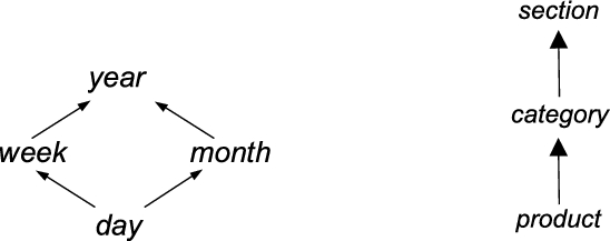
Dimension hierarchies, Time (left) and Product (right).
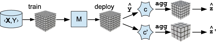
Reframing schema for two multidimensional contexts c and
When the context is fixed, conventional context-insensitive performance metrics (see, e.g., [23]) can be used to evaluate how a model performs for that context. However, when we use the same model for several contexts we need context-aware performance metrics. In this section we discuss how to obtain such metrics and how they can be represented and related to the so-called context plots.
Evaluating a model on a range of contexts
Let us consider how a model (either reframed or not) can be evaluated for a given context. This is represented by a loss function
A model is said to dominate another in a region
We can examine the whole range of operating contexts and see in which regions one model is better than others. However, as dominance may only occur for partial regions, we may wish to have an overall metric accounting for the whole distribution of contexts.
The expected loss of a model m using reframing procedure R over data D and a distribution of contexts w over the space of contexts
If θ contains discrete parameters only, this can be substituted by a weighted sum instead of the integral. Note that we can only talk about a versatile model if it can be successfully reframed (even if not optimally) for a range of contexts. This generalises the approach of [35,37], which reinterprets several known performance metrics previously considered context-insensitive, such as AUC and Brier score, as aggregates over contexts.
Expected loss as defined above requires the estimation of w, the distribution of contexts. Default choices are possible but can be controversial. For instance, in classification there is a long-standing debate about whether the distribution of skews or the cost proportion must be considered uniform or can be modelled with other distributions (for instance, other beta distributions) [27,31].
The visualisation of how the loss Q changes for a range of operating contexts is a context plot:
A context plot shows Q as a function of θ for a given dataset D.
The dimensionality of the plot depends on the number of parameters in θ, ranging from simple one-dimensional curves to complex hypersurfaces. We can plot different models m or different reframing techniques R on the same loss-context space. If we assume
When the context plot has more than two dimensions it can be convenient to represent the plot with a mapping or projection onto a different space
A context reduction is a mapping from
Context plots and context distributions can be extended with context reductions instead of contexts. Context reductions can also be used as transformations to yield a more representative spread on the x-axis, such as applying a logarithmic scale or applying the distribution w over the x-axis [34].
In binary classification, one choice for the context can be the cost proportion
Let us focus for the moment on the simple case where the context is just
We can plot
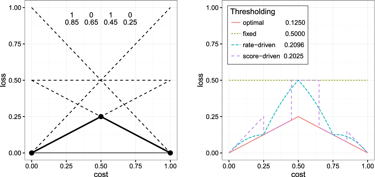
Context plots for binary cost-sensitive classification, where output reframing occurs by means of different threshold choice methods. Left: Cost lines of a simple example. Right: Cost curves obtained by four different threshold choice methods.
Figure 5 illustrates 4 instances with scores (0.85, 0.65, 0.45, 0.25) and actual classes (
Costs are also common in regression. One simple case is the asymmetric loss, where over-estimates and under-estimates have different costs. This can be modelled by a parameter
The asymmetric absolute error
By adding or subtracting a constant value to all predictions we can get better results when α changes, by minimising expected loss. This is another case of output reframing, where the reframing process is expressed again as in Eq. (2).
The loss function here is given by
Note that the above cost-sensitive context plots for binary classification and regression can be derived analytically. For instance, in the context plots shown in Fig. 5, given a classifier, we can calculate all curves in the figure analytically, as they all correspond to an output reframing, and the context-dependent prediction (e.g., a class being predicted after setting a threshold) can be used in Q to compare with the true labels using the context. In this way, given a versatile model (e.g., a probabilistic classifier), we can calculate the area under each curve analytically, without the need of going context by context [36]. Similarly, for regression using cost asymmetry as shown in Fig. 6, the curves can be plotted analytically and their areas can be derived from the model itself.
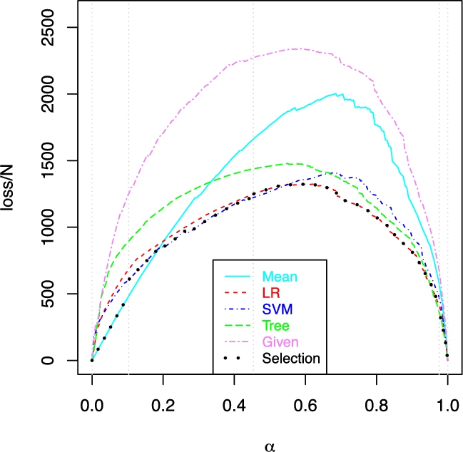
However, in many other cases the context plots cannot be derived analytically. For instance, the context can be defined as a trade-off between misclassification cost (MC) and attribute test cost (TC) with a parameter
Context plot for cost-sensitive regression with α a context parameter trading off between over- and under-estimation penalties, and output reframing through shifting.
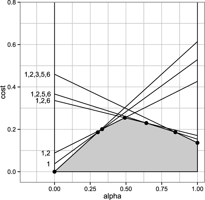
Context plot for cost-sensitive classification with attribute costs and misclassification costs, with α a context parameter trading off between the two.
An interesting future direction is to consider ‘process costs’, that is, to use a performance metric that takes into account the cost of retraining/reframing, having too many models (in ensemble approaches), parametrising the context, etc. Process cost analysis is a problem of increasing importance and the integration of these budgets into machine learning is an active research area [67].
Examples of applications where we should probably consider different contexts during deployment are relatively common. Below we show more cases of context parametrisations, which have been (or could have been) represented as a context plot.
Some of the contexts seen in previous sections may be composed of several parameters (e.g., the coefficient values in some input reframing approaches [3], so θ has twice as many parameters as attributes). In the multidimensional datamart example [46] the operating context is an OLAP cube, and θ is not only composed of many parameters but they are also discrete. These cases lead to more complex context plots, but some representations or simplifications may still be insightful.
Regression Error Characteristic (REC) curves [8] plot the error tolerance on the x-axis versus the percentage of points predicted within the tolerance on the y-axis. Error tolerance may be context-dependent, and in this sense REC curves are another example of context plots.
Comparing reframing and (transductive) transfer learning. Asterisks refer to exceptions for multi-task learning
Comparing reframing and (transductive) transfer learning. Asterisks refer to exceptions for multi-task learning
Like the joint cost case described in the previous section and shown in Fig. 7, most of the context plots in this section are empirical rather than analytic and need to be constructed through experiments. In the input shift example [3] the context affects the input attributes, leading to an output change through the model. As the relation between the inputs and outputs is model-dependent, it is not possible, in general, to derive the curves analytically. This means that we have to sample over operating contexts in order to plot these curves and estimate its area to obtain the expected loss (Definition 4). A similar situation happens where the context is some kind of noise that affects all input attributes, such as the measurement error in several sensors given by temperature [22]. Finally, in the multidimensional contexts example, both a context change in inputs/outputs and an output reframing is required. An analytical derivation of these curves (and their areas) is not possible in general.
The notion of context or domain adaptation has been studied before in machine learning and more generally in computer science. There are several areas that overlap with the notion of reframing under context changes, although for most of them the focus on anticipation and versatile models are absent.
Only cost-sensitive learning and ROC analysis (when there is no retraining) can be seen as areas where reframing has been commonly used in the past, and generally restricted to binary classification. However, many other tasks and applications, especially with the use of input and structural reframing, present themselves as new opportunities.
In the context of these related areas, we are now in a position to highlight the distinctive characteristics of reframing:
Contexts are identified and parametrised. Models are learnt in anticipation of context changes and optimised to behave well in a range of contexts. We do not consider a 1-to-1 transfer from a source problem to a target problem, but a systematic application to multiple contexts. Once the reframing procedure is set, reframing is automated for any deployment data given the context. Even if models are intended to be general and versatile, they are usually learnt in one context and task. It is through the parametrisation of context – a kind of ‘inductive context bias’ – that they are expected to be adapted to other contexts. Models are compared with the notion of dominance for ranges of contexts. Expected performance can be plotted for a range of contexts. Aggregated metrics can be derived. Models are reused. The model is versatile enough to be adapted to several contexts, which avoids the cost of retraining or revision.
There are scenarios where contexts cannot be identified or parametrised, or where the model is not versatile enough. Also, it may happen that we evaluate a versatile model together with a particular reframing mechanism for a distribution of contexts, but have no clear dominance regions so that we have to keep several models or select the one that is best for the expected distribution of contexts. It may turn out that this distribution is different to the one that we finally observe in a deployment setting.
The notion of context parametrisation and its application to reframing seems to be better suited for non-interactive machine learning (supervised, semi-supervised or unsupervised) when there is a true model, but needs to be rethought for other areas of machine learning, such as instance-based learning, and particularly in domain adaptation and transfer learning in reinforcement learning [58].
While it is important to highlight these limitations, this paper has shown that there are many more cases where reframing is possible and useful than just those traditional cases concerning cost-sensitive learning and prior distribution shift already analysed in the case of binary classification using ROC analysis, cost curves and parametrised decision rules.
Concluding remarks
This paper has provided a unified view of a family of solutions for a set of context-change problems under the term reframing. We have generalised the types of context changes in Table 1, clarified the three types of context-aware adaptations in Section 3 and defined a taxonomy of the types of reframing.
In addition to providing common terminology and notation, we hope this paper also enables a better understanding of the commonalities and differences in problems and solutions, as well as identifying ‘niches’ where some of the techniques discussed could be applied or adapted.
Taking a higher-level view, we think that the notion of reframing may have a deeper and more long-term impact in how the process from data to knowledge, its validation and its application to real problems can be conceived. We finish by highlighting the key points underlying this view.
Models should be as general and flexible as possible. The data and conditions used to learn the model may change for each particular application. Versatile models integrate more information than originally needed, such as probabilities, distributions, covariance information, unpruned or alternative rules, etc.
Validation should consider a range of operating contexts, either by analytically integrating them into the validation process, simulating them with data modification or by the use of data from different situations. Furthermore, validation has to take into account that repeatedly learning for each particular application has the risk of overfitting to the operating context.
Related to the previous point, performance metrics that account for a range of situations instead of more short-sighted metrics that only account for one operating context should be the base for a more comprehensive model evaluation.
Learning and assessing models has a cost, so we should always consider the overall costs involved in retraining, revising and reframing. The possibilities and cost of properly identifying the operating context (and when this information will be available) must be considered during the whole process.
Model deployment is a very important stage. Machine learning and data mining applications are not finished when a good model is obtained. The process from data to models is just one part of the game, as the ultimate goal is high-quality decision making. Taking full advantage of a learnt model may require complex decision processes that consider all available information at deployment time.
Footnotes
Acknowledgements
We thank the anonymous reviewers for their comments, which have helped to improve this paper significantly. This work was supported by the REFRAME project, granted by the European Coordinated Research on Long-term Challenges in Information and Communication Sciences Technologies ERA-Net (CHIST-ERA), funded by their respective national funding agencies in the UK (EPSRC, EP/K018728), France and Spain (MINECO, PCIN-2013-037). It has also been partially supported by the EU (FEDER) and Spanish MINECO grant TIN2015-69175-C4-1-R and by Generalitat Valenciana PROMETEOII/2015/013.