Use of symbolic dynamic time warping in hierarchical clustering of urban fabric evolutions extracted from spatiotemporal topographic databases

Abstract

This article introduces a new methodology dedicated to classify the evolutions of urban blocks extracted from spatio-temporal topographic databases where an urban block is defined as the smallest area that is surrounded by communication network (roads, railways, …). To achieve that, an ascendant hierarchical clustering is applied to sequences of urban block states (i.e., sequences of class labels to which the block belongs to at each date). The principal originality of this approach is to use a distance measure based on DTW (Dynamic Time Warping) which is able to apprehend temporal behaviors (mainly time lags in dates corresponding to a change of state) and which takes into account the semantic proximity between the different kinds of urban blocks. Several experiments have been carried out on areas in the city of Strasbourg (France). First results are relevant and highlight realistic urban dynamics.

Keywords

Urban dynamics analysis dynamic time warping symbolic time series clustering

1. Introduction

Analysis of changes in urban and suburban areas over time allows estimating the nature of underlying natural and anthropic processes and to anticipate possible implications in terms of management of natural resources and territories (landscape). Urban sprawl is a universal, although unevenly distributed phenomenon. Its terms are different depending on the area and the period considered. The analysis of the distribution of urban areas at the European level shows that urbanization is taking place intensively in some areas, even though population may decrease or increase slowly. Monitoring urban sprawl and its consequences remains a major challenge for urban planning and management [9,10,12].

Urban fabric characterization is very useful in planning, modeling and simulation and it is an important precondition to better understand the urbanisation process of cities [19]. Nowadays, the availability of historical cartographic databases enables digital change monitoring and analysis of urban fabric characteristics thus replacing visual inspection and interpretation of city plans and maps. These vector databases are analyzed in order to improve the knowledge on specific objects such as buildings and to identify evolution characteristics at different meso-geographical levels (e.g., city or urban block). Some urban studies coming from urban geography research have focused on urban fabric characterization often based on morphometric indicators [3,7,8,19,24]. Few of them are focused on the analysis of their evolutions.

A process to analyse urban block evolutions could consist in classifying automatically urban blocks at each time point according to a predefined classification and then in learning evolutions from these monodate classifications. Unfortunately, from our knowledge, there is not taxonomy of urban block evolution classes which can be used to define the classes which can be considered and to define associated reference data (e.g., ground truth, training samples). As one cannot assume that such reference data are going to be available, methods that are able to process such evolutions in an unsupervised way are needed.

In this context, this paper focuses on the clustering of urban block evolutions extracted from topographic database. The extraction of relevant clusters aims to help the expert in three parts: firstly, for inducing a semantic meaning for them according to his/her expertise domain; secondly for studying each kind of evolution according to characteristics of urban blocks involved in the evolution and, thirdly for identifying representative evolutions (for example, evolutions near to the centres and/or the borders of the clusters) which can be used in supervised algorithm.

Section 2 introduces a global process for clusterize the urban block evolutions based on the use of DTW (Dynamic Time Warping). Section 3 presents the topographic database used and the way to construct the urban block state sequences while Section 4 introduces an adaptation of the DTW to symbolic data and details the similarity matrix used to define the similarities between the different states (i.e., classes) of urban blocks. Experiments carried out on several databases are presented in Section 5. Section 6 concludes this paper and proposes further work.

2. A global process to clusterize urban block evolutions

Clustering is a well-known family of methods which are able to process in an unsupervised way. This family is made up of well-known algorithms like the K-means algorithm or the Ascendant Hierarchical Clustering algorithm. Clustering aims at grouping similar data. In the case of urban dynamic analysis, it would consist of grouping urban block that have a similar evolution. The vast majority of the most used clustering algorithms are based (at least) on a similarity measure, which makes it possible to know how close two data points are. When handling evolution of urban blocks (i.e., sequences of states corresponding each to a thematic class to which the urban block belongs at the considered date), defining a similarity measure is much harder than when handling numerical values in a vector space without natural ordering. There are actually four main problems: firstly, each state of evolution is symbolic, which means that the similarity between different states of evolution have to be defined by the expert.1

¹
In the case of numerical values, the values can be used to evaluate the similarity between the objects to compare.

Secondly, the temporal structure of the data has to be taken into account: an urban block evolving from wasteland to individual housing, is very different than an urban block evolving from individual housing to wasteland. Thirdly, only few databases are available over the last fifty years. Therefore, only methods that deal with irregular temporal sampling will be able to fully exploit all the available databases. Finally, a single urban block (corresponding to a geographic area) can evolve into two blocks and conversely. For instance, in [21], the author combines the land use information and the shapes of regions to characterize the transition patterns from one time point to the next [20]. He proposes six region states according to these aspects: stability, substitution (change of land use), division without land use change, and division with land use change, expansion and conversion. The goal of this work is the dual of ours. The author aims to study the land use transition processes themselves: statistics of transitions associated with each kind of region states for instance. In the same way, [15] defines 25 transition types to analyse vegetation time series.

This paper introduces a global process for clusterize the urban block evolutions based on the use of DTW (Dynamic Time Warping) to address the first three issues and on a linearization of the evolutions into urban block state sequences to address the fourth one. The proposed global process consists in four steps (Fig. 1):

Fig. 1.

Overview of the proposed process.

The area is selectionned by the expert from existing spatio-temporal topographic vector databases, one by year (cf. Section 3). Then, for each date, the urban blocks are built using communication network and are characterized by morphological attributes, by the spatial distribution of buildings and by the open space within a block (cf. Section 3.1).

All the urban blocks are classified using classification model given by the expert (cf. Section 3.1).

A graph of urban block evolution is built. That consists in linking urban blocks from two successive dates which overlap. Then this graph is linearized: a new sequence is built for each path from a block in the first date to a block in the last date. (cf. Section 3.3).

All these sequences are clusterized using DTW (cf. Section 4.3) based on a similarity matrix (cf. Section 4.6) and the Ascendant Hierarchical Clustering Algorithm (cf. Section 4.7).

Note that this global process is implanted in the Area manager plateform as part of the FoDoMuST2

http://icube-sdc.unistra.fr/fr/index.php/Plateformes.

plateform dedicated to classification of time series mainly remote sensing images, symbolic data and texts [5]. Figure 2 shows the scheme of the FoDoMuST plateform.

Fig. 2.

The FoDoMuST plateform with three interfaces (Classifx dedicated to ARFF file classification, AreaManager – iVisualize dedicated to topographic databases classification, Mustic dedicated to remote sensing image classification) and two libraries (JCL – Java Clustering Library and JCL – Java Segmentation Library).

3. Material

3.1. Spatio-temporal topographic vector database

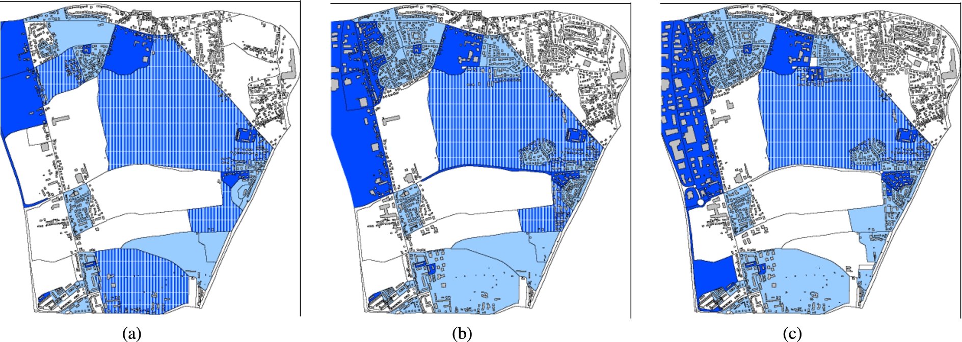
In this study, the geographic objects contained within the topographic databases (BDTOPO®IGN) produced by the French National Institute of Geography (IGN) are used as benchmark data. A such topographic database is, for a given date, a vector 3D description (structured objects) elements of the territory and its infrastructure, at meter accuracy, exploitable at scales ranging from 1:5000 to 1:50,000. Historic databases are then created for four test areas with the following six different dates: 1956, 1966, 1976, 1989, 2002 and 2008. These four zones are chosen because they have been subject to a variety of typical urbanisation processes. For example, the area presented in this paper (Fig. 3(a), (b), (c)) corresponds to a typical expansion phenomenon called peri-urbanisation phenomenon. It is also subject to natural constraints (rise of ground water) in the centre. This area is localized in the North of Strasbourg3

³
GSP coordinates: ⟨longitude: 7.739455223462405 ; longitude: 48.61865888192552; altitude: 0⟩.

(France).

The proposed typology of urban blocks (Table 1) is compatible with existing land-cover/use nomenclature (e.g., Corine Land Cover). It is adapted to map the territory at the scale of 1:10,000.

3.2. Urban block construction

For each date independently, the urban blocks are built automatically using communication objects (road, railways and hydrographic networks) available in the topographic database. For each date, the set of blocks totally covers the study area (without holes or overlap). All the urban blocks are then labelled automatically by a supervised classification process which was only based on the morphological attributes and, the spatial distribution of buildings and the open space within a block. All the details about the method used to label the urban blocks are given in [16,24].

Fig. 3.

Figure 4 gives an example of PMML4

⁴

The Predictive Model Markup Language (PMML) is an XML-based language to define statistical and data mining models. More information about PMML can be found at http://www.dmg.org.

file (containing the predictive model) given as input to the processus of classification implanted in the Area manager plateform. Omission and commission errors in all the classifications have been manually corrected by an expert in urban planning (Fig. 3(b), (d), (f)).

3.3. Construction of sequences

The aim of the work presented in this paper is to classify evolutions of urban blocks i.e., to classify their sequences of states. Each of these states corresponds to the class to which the block belongs at the considered date (see Section 3.2).

However, several changes can appear over an area, like the building (resp. the removal) of a road. By assumption, roads/railways/… form the boundaries of urban blocks (as urban blocks are surrounded by communication ways) and therefore building (resp. the removal) of a road/railways/... can split (resp. merge) urban blocks.

For instance, in Fig. 5, where ${(b_{i}, C_{k})}^{t}$ denotes that the label associated to urban block $b_{i}$ is $C_{j}$ at date t, urban block $b_{1}$ is split into $b_{2}$ and $b_{3}$ between $t = 1$ and $t = 2$ while urban blocks $b_{4}$ and $b_{5}$ are merged into $b_{6}$ between $t = 3$ and $t = 4$ . Thus, we have to deal with an oriented graph of urban blocks evolutions instead of simple linear evolutions. In order to classify the sequences, this graph is linearised by taking into account all the paths from a block at the first date to a block at the last date. For instance, from the example in Fig. 5, three sequences are built:

${{(b_{1}, C_{1})}^{1}, {(b_{2}, C_{1})}^{2}, {(b_{4}, C_{1})}^{3}, {(b_{6}, C_{7})}^{4}, {(b_{7}, C_{3})}^{5}}$ ;

${{(b_{1}, C_{1})}^{1}, {(b_{2}, C_{1})}^{2}, {(b_{5}, C_{5})}^{3}, {(b_{6}, C_{7})}^{4}, {(b_{7}, C_{3})}^{5}}$ ;

${{(b_{1}, C_{1})}^{1}, {(b_{3}, C_{3})}^{2}, {(b_{3}, C_{3})}^{3}, {(b_{3}, C_{3})}^{4}, {(b_{7}, C_{3})}^{5}}$ .

In the sequel of the paper, as only the labels of class are taken into account in the classification process, the notation used to describe sequence is simplified into

C k_{1} > C k_{2} > \dots > C k_{i} > \dots > C k_{n}

, where

C k_{i}

is the class associated to the ith state of the sequence and n the length of the sequence (e.g.,

C 1 > C 1 > C 5 > C 7 > C 3

n = 5

). One can notice that a block can belong to several sequences and, as will be shown in Section 5, it can belong to several kinds of evolution since the sequences (where it appears) can be classified into different clusters. Nevertheless, we assume that this is not a problem because the aim of the process is to highlight classes of evolution and not individual block behaviour.

Table 1
Urban blocks classes

# Class name

$C_{1}$ Dense urban fabric (e.g., city centre)

$C_{2}$ Discontinuous urban fabric with housing blocks

$C_{3}$ Discontinuous urban fabric with individual houses

$C_{4}$ High density of mixed urban fabric (mixed of $C_{2}$ and $C_{3}$ )

$C_{5}$ Low density of mixed urban fabric (mixed of $C_{2}$ and $C_{3}$ )

$C_{6}$ High density of mixed areas (including $C_{2}, C_{3}$ and $C_{8}$ )

$C_{7}$ Low density of mixed areas (including $C_{1}, C_{2}, C_{3}$ and $C_{8}$ )

$C_{8}$ High density of specialised areas (e.g., industrial, commercial, hospital or scholar buildings)

$C_{9}$ Low density of specialised areas (e.g., few or no buildings or wasteland)

$C_{10}$ Communication network (e.g., roads, country roads, railroads)

$C_{11}$ Hydrographic network (e.g., canals, rivers)

#	Class name
$C_{1}$	Dense urban fabric (e.g., city centre)
$C_{2}$	Discontinuous urban fabric with housing blocks
$C_{3}$	Discontinuous urban fabric with individual houses
$C_{4}$	High density of mixed urban fabric (mixed of $C_{2}$ and $C_{3}$ )
$C_{5}$	Low density of mixed urban fabric (mixed of $C_{2}$ and $C_{3}$ )
$C_{6}$	High density of mixed areas (including $C_{2}, C_{3}$ and $C_{8}$ )
$C_{7}$	Low density of mixed areas (including $C_{1}, C_{2}, C_{3}$ and $C_{8}$ )
$C_{8}$	High density of specialised areas (e.g., industrial, commercial, hospital or scholar buildings)
$C_{9}$	Low density of specialised areas (e.g., few or no buildings or wasteland)
$C_{10}$	Communication network (e.g., roads, country roads, railroads)
$C_{11}$	Hydrographic network (e.g., canals, rivers)

4. Symbolic dynamic time warping

When studying the evolution of urban areas over time, the core of the process generally consists of comparing data in order to estimate (dis)similarity. The distance provides an estimation of this similarity.

When the data is temporal, the choice of the distance is crucial since it completely defines the way of tackling the temporality of the data. This dissimilarity measure must exploit the temporal distortions and compare shifted or distorted evolution profiles. It must be able to deal with sequences whose time sampling is irregular.

In this paper, we define and propose to use such a similarity measure which is a mix between the Edit-distance (also known as Levenshtein distance) [17] and Dynamic Time Warping (DTW), based on the Edit-distance and introduced in [27,28].

Fig. 4.

An example of PMML file.

Fig. 5.

Graph of urban block evolutions (5 dates). ${(b_{i}, C_{k})}^{t}$ denotes that the label associated to urban block $b_{i}$ is $C_{j}$ at date t.

In order to present the similarity measure used in this work, let us first define these two measures. Throughout this section, let $A = ⟨ a_{1}, \dots, a_{N_{a}} ⟩$ and $B = ⟨ b_{1}, \dots, b_{N_{b}} ⟩$ be two sequences of characters (two strings) or of values depending upon the situation. In our case as the set of blocks totally covers the entire study area (without holes or overlap) at each date, each urban block has at least a corresponding urban block at the next date. Then $N_{a} = N_{b}$ but it is not always the case. For instance, if the sequences are built from remote sensing images, some values can missed due to clouds on a part on of the scene at different times.

4.1. Definition

4.2. Levenshtein distance

The Levenshtein or edit distance [17] formalises the notion of distance between two character strings, by focusing on transforming (or editing) one string into the other by a series of edit operations on individual characters. This distance requires a similarity matrix between letters to know which characters are close to each other and which are not. The permitted edit operations are the insertion, deletion and replacement of a character. The cost of the transformation from one string to another can be recursively computed by: $\begin{array}{l} D (A_{i}, B_{j}) \\ (1) & = min \{\begin{matrix} D (A_{i - 1}, B_{j - 1}) + sim (a_{i}, b_{j}), \\ D (A_{i}, B_{j - 1}) + del (b_{j}), \\ D (A_{i - 1}, B_{j}) + ins (a_{i}), \end{matrix} \end{array}$ where $A_{i}$ is the sub-sequence $⟨ a_{1}, \dots, a_{i} ⟩$ , $i ⩽ N_{a}$ and $a_{i}$ is the ith character of the string A. Moreover, functions $ins$ , $del$ and $sim$ are generally defined as:

$\forall c : character, del (c) = ins (c) = 1$ i.e., the deletion and insertion of a character is constant and equal to one;

$sim$ is a similarity matrix between all characters of the vocabulary.

The overall similarity is given by

D (A_{N_{a}}, B_{N_{b}})

4.3. Dynamic time warping

Dynamic Time Warping (DTW) is based on the Levenshtein distance and was introduced in [27,28], with applications in speech recognition. It is probably the most commonly used measure to quantify the dissimilarity between numerical sequences [1,2,6,22,23,26,29]. It finds the optimal alignment (or coupling) between two sequences of numerical values, and captures flexible similarities by aligning the coordinates inside both sequences. The cost of the optimal alignment can be recursively computed by: $\begin{array}{l} D (A_{i}, B_{j}) = & sim (a_{i}, b_{j}) \\ (2) & + min \{\begin{matrix} D (A_{i - 1}, B_{j - 1}), \\ D (A_{i}, B_{j - 1}), \\ D (A_{i - 1}, B_{j}) . \end{matrix} \end{array}$

Figure 6(a) shows such optimal alignements of three sequences. From this figure, one can notice that:

A and B are less similar than B and C even if lengths of A and B are equal and that of C is smaller.

The cost to align $a_{3}$ and $b_{2}$ is null even if the states are not considered at the same date

In the subsequence $⟨ c_{2}, c_{3} ⟩$ , the two states are from a same class C, that may mean that the corresponding urban block had the same state between $T_{c_{2}}$ and $T_{c_{3}}$ . These states are associated with a state of the class C from B with a null cost.

if DTW aligns two states of same class from two sequences $S_{x}$ and $S_{y}$ , the date and the duration of theses states (i.e., the number of consecutive states of same class in $S_{x}$ and $S_{y}$ evolved in this alignement) have not impact the similarity.

In other words, on the one hand, DTW can deal with sequences having different lengths and so deal with missing data. In our case, databases covered by our method (and used in our experiments) have normally not missing data. Reader interested by this aspect, can find an example dealing with such data in [22]. On the other hand, it gives a chronological view of the phenomena rather than a chronometrical one. In the case of urban evolution, this property is very interesting. For instance, densification of a urban block is often composed of different keysteps: individual houses demolition, vegetation clearance, removal of soil, building construction, development of green spaces, …which can correspond to the sequence of states: C3 > C9 > C5 > C2 (Table 1) regardless (1) the date of transformation starting and (2) duration of each state. Figure 6(a) shows two such sequences B and C. These two sequences represent the same urbanization process. For the DTW measure they are very similar while the Euclidean measure, where the missing states in sequence C are supposed identical to the last one in the sequence, gives a value equals to 8 (Fig. 6(b)).

Fig. 6.

Distance between three sequences calculated using DTW and Euclidean distance. (a) Using DTW. (b) Using Euclidean distance (the missing states in sequence C are supposed identical to the last one in the sequence).

However, a direct implementation of this recursive definition leads to an algorithm that has exponential cost in time. Fortunately, the fact that the overall problem exhibits overlapping sub-problems allows for the memorization of partial results in a matrix, which makes the minimal-weight coupling computation a process that costs $| A | \times | B | = N_{a} \times N_{b}$ basic operations. This measure has thus a time and a space complexity of $O (| A | \times | B |)$ .

DTW is mostly used in order to align sequences of numerical values, with $sim$ being the Euclidean distance between the two values.

4.4. Related work

In [4], studies are conducted to compare different (dis)similarity measures. In particular, elastic measures as DTW and edit-based measures are compared to classical L-norms and longest common subsequence. Based on their experiments, the authors conclude that the accuracy of elastic measures converges with that of Euclidean distance as the size of the training set increases. On small data sets, elastic measures can be significantly more accurate than Euclidean distance and other lock-step measures, e.g., $L_{\infty}$ . Reference [25] proposes a method to search and to mine trillions of time series subsequences by using DTW. The authors point out that most time series mining algorithms make extensive use of similarity comparisons and that there is increasing evidence that the classic Dynamic Time Warping (DTW) distance measure is the best one for dissimilarity calculations.

The use of DTW as a similarity measure in clustering technique [23] is relatively classical now. For instance, [14] proposes a density-based clustering using DTW to analyse climate change. Reference [22] shows benefits to using such similarity measure in satellite image time series analysis. In [30], DTW is applied to extract and represent the dynamic mobility patterns in different urban areas. More recently, [11] proposes some alternatives to fuzzy clustering methods to time series analysis based on the DTW distance and on the fuzzy C-means algorithm. Reference [18] presents a time-weighted version of the dynamic time warping method for land-use and land-cover classification using remote sensing image time series. It modifies the DTW method to include a temporal weight that accounts for seasonality of land-cover types. As one can notice, the main uses of DTW are in remote sensing image analysis domain and more rarely for the analysis of topographic databases as in our case.

4.5. The proposed similarity measure

In this work, we propose to combine these two ways of computing a similarity measure between two sequences of characters. As the objective is to compare evolutions of urban fabrics over time, all the states of evolution are used. As such, an adaptation of the Levenshtein distance is used in which no skips are permitted and which is close to DTW. Furthermore, DTW was adapted to sequences of symbols (instead of numerical values) and as the Euclidean distance cannot be applied in this setting, the states were compared using as $sim$ function a similarity based upon the thematic classes of urban fabric. The proposed sequence similarity measure, called Symbolic Dynamic Time Warping (SDTW) for convenience, is defined in Eq. (2), with A and B being two sequences of evolution of urban fabrics and $sim$ being a similarity matrix between states of urban fabrics. Section 4.6 introduces the similarity matrix used in the experiments. Algorithm 1 details the computation of SDTW.

Algorithm 1

Symbolic Dynamic Time Warping

4.6. Urban block class similarity matrix

A distance of 1 means that classes are close in terms of composition and that the probability to confuse them is very high. A high distance means that classes have no similarity. For example, the similarity between $C_{1}$ (continuous urban fabric areas) and $C_{4}$ (high density of mixed urban fabric) is lower than the similarity between $C_{1}$ and $C_{9}$ (low density of specialized areas). By construction, the similarity matrix is symmetric because the distance evaluates only the “semantic difference” between $C_{i}$ to $C_{j}$ and not the cost of transition from state $C_{i}$ to $C_{j}$ which can be different of the cost of the transition from state $C_{j}$ to $C_{i}$ .

In order to evaluate the quality of the matrix, we have calculated the Euclidean distance between all classes based on attributes on buildings of each block (size, shape, elongation, number of buildings per block, etc.). It appears that the proposed semantic distance is close to the Euclidean distance. Nevertheless, some validations are still necessary but we assume that this study is out of the scope of this paper.

4.7. Ascendant hierarchical clustering

A lot of clustering algorithms exist [13]. Partitioning algorithms generates flat partitions of the data, i.e., sets of clusters (or groups). The clusters can be disjoints (hard clustering), can be overlapped (soft clustering) or be defined using degrees of membership (fuzzy clustering). Hierarchical algorithms produce hierarchies of clusters and present a lot of intrinsic advantages:

They do not require a pre-defined number of clusters: the user can select the “right” number of cluster by pruning the hierarchy manually or using (semi-) automatic methods;

They can work directly with a similarity matrix which can be pre-processed (offline). As they does not need the data themselves in the clustering process (inline), the memory requirements are reduced. It is also especially interesting in case of information are private or not accessible (medical data, banking data, …);

They do not require averaging method to calculate centers of cluster (as in the well-known K-means algorithm).

For the user, a representation of such hierarchy by a dendrogram seems more natural than flat representation and, then, simplify the understanding of the results. Nevertheless, one of the main drawbacks lies in the choice of cutting the tree. Indeed, as introduced in [13], (1) clustering algorithms find clusters, even if there are no natural clusters in the data and (2) each algorithm, implicitly or explicitly, imposes a structure on the data: if the match is “good”, algorithm is successful. Thus, without any examples, ground truth, model or typology of urban block evolutions, it is very difficult to quantify quality of clustering. Only qualitative quality can be evaluated. The only way to do that, is then to use knowledge of the expert and his/her ability to cut the tree so that the clusters are meaningful to him/her.

The Ascendant Hierarchical Clustering (AHC) performs clustering in four steps:

Begin with groups containing only one basic instance (i.e., N groups of one sequence where N is the number of constructed sequences at the previous step).

Compute (or update) the similarity (or the distance) between every group pair in a triangular matrix $M_{dis}$ using a given linkage criterion.

Merge the two closest groups5

⁵
If there are more than two groups, two are randomly chosen among them.

(i.e., the groups which have the greatest similarity (or lowest distance) value in

M_{dis}

), and modify

M_{dis}

accordingly (by merging the two lines/columns associated to these two groups).

If there are more groups than desired (generally, one group), go to step 2.

This algorithm hierarchically builds clusters of sequences while minimizing their intra-group variance. The linkage criterion determines the similarity (or the distance) between two clusters $C_{i}$ and $C_{j}$ as a function of the pairwise similarity (or distances $dist$ ) between objects belonging to the clusters. The single-linkage $\begin{array}{l} SL (C_{i}, C_{j}) \\ = min (dist (o_{a}, o_{b}), o_{a} \in C_{i}, o_{b} \in C_{j}) \end{array}$ is able to find non convex clusters but it is highly sensible to noise or to outliers. The complete-linkage $\begin{array}{l} CL (C_{i}, C_{j}) \\ = max (dist (o_{a}, o_{b}), o_{a} \in C_{i}, o_{b} \in C_{j}) \end{array}$ is less sensible to noise or to outliers but it tends to create small clusters. The average linkage $\begin{array}{l} AL (C_{i}, C_{j}) \\ = \frac{1}{| C_{i} | \cdot | C_{j} |} \sum_{o_{a} \in C_{i}} \sum_{o_{b} \in C_{j}} max (dist (o_{a}, o_{b})) \end{array}$ between two cluster $C_{i}$ and $C_{j}$ is few sensible to noise or to outliers but it is mainly used to find convex clusters. Thus, it seems a good compromise between the two others linkage criteria. In fact, in our experiments, we have chosen to use the average linkage criterion.

In the case of time series analysis using SDTW, it is defined by: $\begin{array}{l} AL (C_{i}, C_{j}) \\ (3) & = \frac{1}{N_{i} \times N_{j}} \sum_{a = 1}^{N_{i}} \sum_{b = 1}^{N_{j}} SDTW (S_{a}, S_{b}), \end{array}$ where $N_{i}$ (resp. $N_{j}$ ) is the number of sequences in the cluster $C_{i}$ (resp. $C_{j}$ ) and where $S_{a} \in C_{i}$ and $S_{b} \in C_{j}$ . The linkage value between two clusters that contain single sequence each is defined as the SDTW measure between these sequences.

By construction, the obtained hierarchy is a binary tree of clusters. It is usually modeled as a simple binary tree or as a dendrogram. In the case of the simple tree, there is no information about the distance between the two children of a node while in a dendrogram, the length of a branch is related to this distance. In our case, even if we calculate (and present to the expert) the dendogram, these distances are not used to evaluate evolutions associated with each cluster. In fact, we do not report the numerical values on all the figures.

Fig. 7.

No equal sequences having a DTW value equals zero and the associated average sequence.

Remark: DTW is not a distance because $DTW (A, B)$ can be zero even if A differs to B. Figure 7 (on the top) shows a such example. In fact, the theoretical requirements of AHC regarding ultrametric properties are not guaranty.6

⁶

But, we have never encounter in our experiences cases where DTW fails to build such a hierarchy. Nevertheless, this theoretical aspect should be studied but that it is out of the scope of this paper.

Thus, although in general leaves contain only one sequence, we decide to group, in a preprocessing step, all the sequences having a DTW value equals to zero into a leaf. Then, each of these leaves is summarized by the average sequence, i.e., the unique sequence (1) having a DTW value equals zero with all the sequences belonging to the leaves and (2) presenting the minimal length. Figure 7 (in the bottom) shows a such average sequence. One can notice that this sequence only provides a chronology of the states through which the sequences are passed through (see Section 4.3). It does not present necessary the same length than the initial sequences.

Finally, the ascendant hierarchical clustering starts from theses leaves: on all the figures, we report only the average sequences as leaves.

For readability purpose, we index the two childrens of a node by <name of the node>.1 and <name of the node>.2. The name of the root is E.

Figure 8 shows the top of the cluster hierarchy obtained on our dataset with the ratio of objects in each cluster.

Fig. 8.

The top of the cluster hierarchy. The value associated with a branch corresponds of the percentage of sequences in the subclass.

5. Results and discussions

To assess the relevance of our method for the analysis (i.e., the identification) of the principal blocks evolutions, several experiments have been carried out on an area in the city of Strasbourg (France) representing a surface of around 15 km². Figure 3 shows three dates out the five ones. The number of urban blocks increases from less than 50 in 1956, to 74 in 1976, 105 en 1989, 130 in 2002 and finally around 140 in 2008.

The experiments consisted of applying the Ascendant Hierarchical Clustering algorithm on the urban block sequences using the proposed SDTW and the similarity matrix described in Table 2. The obtained hierarchy is pruned by an expert (see Section 4.7) according to the thematic evolution classes he/she looks for. Figure 8 depicts the top of the obtained hierarchy while Fig. 9(a) and (b) focuse on the two sub-clusters from $E_{1.1}$ (namely $E_{1.1.1}$ and $E_{1.1.2}$ ) kept by the expert as having sense in his/her domain.

Table 2
Dissimilarity matrix between urban block classes

$C_{1}$ $C_{2}$ $C_{3}$ $C_{4}$ $C_{5}$ $C_{6}$ $C_{7}$ $C_{8}$ $C_{9}$ $C_{10}$ $C_{11}$

$C_{1}$ 0 1 3 2 3 2 3 1 4 4 4

$C_{2}$ 0 2 2 2 1 1 2 4 4 4

$C_{3}$ 0 2 1 3 3 3 4 4 4

$C_{4}$ 0 1 1 2 3 4 4 4

$C_{5}$ 0 2 1 3 4 4 4

$C_{6}$ 0 1 2 4 4 4

$C_{7}$ 0 2 3 4 4

$C_{8}$ 0 3 4 4

$C_{9}$ 0 2 2

$C_{10}$ 0 3

$C_{11}$ 0

	$C_{1}$	$C_{2}$	$C_{3}$	$C_{4}$	$C_{5}$	$C_{6}$	$C_{7}$	$C_{8}$	$C_{9}$	$C_{10}$	$C_{11}$
$C_{1}$	0	1	3	2	3	2	3	1	4	4	4
$C_{2}$		0	2	2	2	1	1	2	4	4	4
$C_{3}$			0	2	1	3	3	3	4	4	4
$C_{4}$				0	1	1	2	3	4	4	4
$C_{5}$					0	2	1	3	4	4	4
$C_{6}$						0	1	2	4	4	4
$C_{7}$							0	2	3	4	4
$C_{8}$								0	3	4	4
$C_{9}$									0	2	2
$C_{10}$										0	3
$C_{11}$											0

Figure 10 (resp. Fig. 11) illustrates the maps corresponding to the cluster $E_{1.1.1}$ (resp. $E_{1.1.2}$ ). In these figures and all those following, for the sake of readability, only the three most representative dates in terms of evolution are shown: the evolution shown in figure begins later than that presented in the two figures. That explains the shift. A block of a particular date is coloured if it belongs to at least one sequence of the considered cluster.7

⁷

Note that the colours have been randomly chosen and thus do not represent semantics information.

For instance, all non-white blocks in Fig. 10 correspond to urban blocks belonging to at least one sequence in cluster

E_{1.1.1}

Moreover, the first (resp. second) child is coloured in dark (resp. in light). For instance, in Fig. 10, sub-cluster $E_{1.1.1.1}$ is coloured in dark orange while sub-cluster $E_{1.1.1.2}$ is coloured in light orange. Finally, the hatched texture highlights blocks that belong to both subclusters, e.g., to $E_{1.1.1.1}$ and $E_{1.1.1.2}$ (resp. to $E_{1.1.2.1}$ and $E_{1.1.2.2}$ ). For instance, the big urban block to the south (Fig. 11(a)) has been splitted into two sub-blocks between 1976 and 1986 (Fig. 11(b)). Thus, two sequences are built. The small block moves into C2 while the second one remains of the original class: the two sequences belong to two different clusters (namely $E_{1.1.2.1}$ and $E_{1.1.2.2}$ ). Thus, the orginal urban block belongs to these two clusters. It is hatched.

In the same way, Fig. 12 illustrates the map corresponding to the cluster $E_{1.1}$ where the two sub-clusters $E_{1.2.1}$ and $E_{1.2.2}$ are coloured in green. The evolution shown in this figure begins later than that presented in the previous two. This explains the discrepancy in dates.

Fig. 9.

Decomposition of the cluster $E_{1.1}$ into deux subclusters. (a) Cluster E.1.1.1. (b) Cluster E.1.1.2.

Fig. 10.

Maps corresponding to the cluster $E_{1.1.1}$ (a) (1976); (b) (1989); (c) (2002).

Fig. 11.

Maps corresponding to the cluster $E_{1.1.2}$ (a) (1976); (b) (1989); (c) (2002).

Fig. 12.

Maps corresponding to the cluster $E_{1.2}$ (a) (1989); (b) (2002); (c) (2008).

Several distinctive evolutions can be extracted from the clustering of urban blocks evolutions. Thus, cluster $E_{1.1}$ seems to correspond to blocks with a densification of buildings and cluster $E_{1.2}$ to blocks with almost no evolution.

In Fig. 10(a)–(c) the evolution corresponds to the transformation of “low density mixing/urban fabric and area” ( $C_{5}$ and $C_{7}$ ). With the dark orange colour, one can observe the evolution of such areas into “high density mixed areas” ( $C_{6}$ ) while with the light orange colour, one can observe their evolution into “discontinuous urban with individual houses” ( $C_{3}$ ).

In Fig. 11(a)–(b), the evolution corresponds to the transformation of areas with no or few buildings ( $C_{9}$ ). With the dark blue colour, one can observe the transformation of such areas into “low density of mixed areas“ ( $C_{7}$ ) while in light blue, one can observe their transformation into “Discontinuous urban with individual houses area“ ( $C_{3}$ ). Note that the difference to the previous evolution in light orange is the initial state of the blocks ( $C_{5}$ or $C_{7}$ vs $C_{9}$ ). The hatched dark and light orange block on the 1976 map belongs to the two clusters because, between 1976 (Fig. 10(a)) and 1989 (Fig. 10(b)), it has been split into seven blocks: the sub-block in the East has moved to $C_{9}$ while the others have moved to $C_{3}$ .

In Fig. 12 one can see blocks with low evolution, mainly roads and non-buildable areas shaded with green. The big block on the left appears in green in 1986 because it is the “father” of the small block corresponding to the roads on the left (2002 and 2008). The hatched dark and light blue block in the South (Fig. 11(a)) has been split between 1976 and 1989 into a block belonging to $C_{2}$ and a block belonging to $C_{5}$ (Fig. 11(b)). (The same for a block in the East and another in the North-West, both of which have been split between 1989 and 2002). The big block in the middle of the map (corresponding to the area subjected to the rise of the ground water) has been merged with its left neighbour between 2002 and 2008.

In these figures, one can see a very small urban block (localized at the far north, in the middle of the area). This block belongs to $C_{4}$ cluster in all dates. This is the only block with this behaviour: it is the only element of $E_{2}$ .

According to theses observations, it is assumed that two-thirds of the

E_{1}

cluster corresponds to blocks which have become denser between 1956 and 2008 and one-third of the cluster to blocks with low (or no) evolution. The

E_{2}

cluster corresponds to the (very small) urban block (localized in the middle of the area corresponding to the area submitted to the rise of the ground water), which is only classed in

C_{4}

for each date (no change).

6. Conclusion

This article has presented a new methodology dedicated to extracting the evolution of urban blocks from spatio-temporal topographic databases. The principal originality of this approach is to use a distance measure (SDTW) which is able to apprehend temporal behaviours (mainly time lags in dates corresponding to a change of state) and which takes into account the semantic proximity between the different kinds of urban blocks. To validate this approach, an ascendant hierarchical clustering has been applied to sequences of block states (i.e., class labels) using SDTW. The class labels associated to the blocks on each date have been pre-calculated by applying a supervised algorithm to the database corresponding to the specific date. The results of the experiment have been studied by an expert and seem to correspond to the reality. This validates the relevance of the proposed methodology. Nevertheless, some additional experiments should be conducted to precisely quantify and identify the evolution patterns of one or more periods.

This work opens up several perspectives and different research directions. From a methodological point of view, we plan to study more formally (1) the definition of the blocks and of the sequences and (2) the quality of blocks and sequences built in order to evaluate their influences on the results. We also plan to compare this approach with K-means-based methods and to use the DTW Barycentric Averaging (DBA) [23] to do that.

Furthermore, it could be relevant to integrate an approach that enables the user to build the similarity matrix. Indeed, by asking the user for different constraint examples between the data (e.g., must-link or cannot-link constraints), semi-supervised clustering approaches could be used to learn/estimate the different values of the matrix.

From an applicative point of view, this methodology could be used for supervised classification (using the K-Nearest Neighbour algorithm for example). Although to define examples seems a difficult and time-consuming task that would require better theoretical definitions of the types of evolution.

Footnotes

Acknowledgements

The authors would like to thank the French National Research Agency (ANR) for having supported the GeOpensim (ANR-08-RAN52-Geopensim) and COCLICO (ANR-12-MN001-COCLICO) projects.

References

Aach and

G.M.

Church, Aligning gene expression time series with time warping algorithms, Bioinformatics17(6) (2001), 495–508. doi:10.1093/bioinformatics/17.6.495.

Bar-Joseph,

Gerber,

D.K.

Gifford,

T.S.

Jaakkola and

Simon, A new approach to analyzing gene expression time series data, in: RECOMB: Proceedings of the Sixth Annual International Conference on Computational Biology, New York, NY, USA, 2002, pp. 39–48. doi:10.1145/565196.565202.

Boffet and

Serra, Identification of spatial structures within urban blocks for town characterization, in: 20th International Cartographic Conference, Vol. 3, 2001, pp. 1974–1983.

Ding,

Trajcevski,

Scheuermann,

Wang and

Keogh, Querying and mining of time series data: Experimental comparison of representations and distance measures, Proc. VLDB Endow.1(2) (2008), 1542–1552. doi:10.14778/1454159.1454226.

Gançarski and

A.-D.

Salaou, Fouille de données multi-stratégie multi-temporelle, in: Journées Francophones sur L’Extraction et la Gestion des Connaissances – Session Démontration, 2016.

D.M.

Gavrila and

L.S.

Davis, Towards 3-D model-based tracking and recognition of human movement: A multi-view approach, in: IEEE International Workshop on Automatic Face- and Gesture-Recognition, 1995, pp. 272–277.

Hamaina,

Leduc and

Moreau, Bridging the geographic information sciences, in: Towards Urban Fabrics Characterization Based on Buildings Footprints, Lecture Notes in Geoinformation and Cartography, 2012, pp. 327–346.

Hermosilla,

Ruiz,

Recio and

Cambra-López, Assessing contextual descriptive features for plot-based classification of urban areas, Landscape and Urban Planning106(1) (2012), 124–137. doi:10.1016/j.landurbplan.2012.02.008.

Herold,

Scepan and

K.C.

Clarke, The use of remote sensing and landscape metrics to describe structures and changes in urban land uses, Environment and Planning A34 (2002), 1443–1458. doi:10.1068/a3496.

10.

Huang,

X.X.

Lu and

J.M.

Sellers, A global comparative analysis of urban from: Applying spatial metrics and remote sensing, Landscape and Urban Planning82 (2007), 184–197. doi:10.1016/j.landurbplan.2007.02.010.

11.

Izakiana,

Pedrycza and

Jamal, Fuzzy clustering of time series data using dynamic time warping distance, Engineering Applications of Artificial Intelligence39 (2015), 235–244. doi:10.1016/j.engappai.2014.12.015.

12.

J.A.G.

Jaeger and

Schwick, Improving the measurement of urban sprawl: Weighted urban proliferation (WUP) and its applications to Switzerland, Ecological Indicators38 (2014), 294–308. doi:10.1016/j.ecolind.2013.11.022.

13.

A.K.

Jain, Data clustering: 50 years beyond k-means, Pattern Recogn. Lett.31(8) (2010), 651–666. doi:10.1016/j.patrec.2009.09.011.

14.

Kremer,

Gunnemann and

Seidl, Detecting climate change in multivariate time series data by novel clustering and cluster tracing techniques, in: 2010 IEEE International Conference on Data Mining Workshops, 2010, pp. 96–97. doi:10.1109/ICDMW.2010.39.

15.

Kulik,

K.S.

Hornsby and

I.D.

Bishop, Modeling geospatial trend changes in vegetation monitoring data, Computers, Environment and Urban Systems35 (2011), 45–56. doi:10.1016/j.compenvurbsys.2010.05.006.

16.

Lesbegueries,

Lachiche,

Braud,

Skupinski,

Puissant and

Perret, A platform for spatial data labeling in an urban context, in: Geospatial Free and Open Source Software in the 21st Century,

Bocher and

Neteler, eds, Lecture Notes in Geoinformation and Cartography, Vol. 4, Springer, Berlin, Heidelberg, 2012, pp. 49–62. doi:10.1007/978-3-642-10595-1_4.

17.

V.I.

Levenshtein, Binary codes capable of correcting deletions, insertions, and reversals, Soviet Physics Doklady10 (1965), 707–710.

18.

Maus,

Câmara,

Cartaxo,

Sanchez,

F.M.

Ramos and

G.R.

de Queiroz, A time-weighted dynamic time warping method for land use and land cover mapping, IEEE Journal of Selected Topics in Applied Earth Observations and Remote Sensing9(8) (2016), 3729–3739.

19.

Meinel,

Hecht and

Herold, Analyzing building stock using topographic maps and gis, Building Research & Information37(5–6) (2009), 468–482. doi:10.1080/09613210903159833.

20.

Mizutani, Land use transition process analysis using polygon event and polygon status: A case study of Tsukuba science city, in: Proceedings of 17th International Conference on Geoinformatics, 2009, pp. 1–6.

21.

Mizutani, Construction of an analytical framework for polygon-based land use transition analyses, Computers, Environment and Urban Systems36(3) (2012), 270–280. doi:10.1016/j.compenvurbsys.2011.11.004.

22.

Petitjean,

Inglada and

Gançarski, Satellite image time series analysis under time warping, IEEE Transactions on Geoscience and Remote Sensing50(8) (2012).

23.

Petitjean,

Ketterlin and

Gançarski, A global averaging method for dynamic time warping, with applications to clustering, Pattern Recognition44(3) (2011), 678–693. doi:10.1016/j.patcog.2010.09.013.

24.

Puissant,

Skupinski,

Lachiche,

Braud and

Perret, Classification et évolution des tissus urbains à partir de données vectorielles, Revue Internationale de Géomatique4 (2011), 513–532. doi:10.3166/rig.15.513-532.

25.

Rakthanmanon,

Campana,

Mueen,

Batista,

Westover,

Zhu,

Zakaria and

Keogh, Searching and mining trillions of time series subsequences under dynamic time warping, in: Proceedings of the 18th ACM SIGKDD International Conference on Knowledge Discovery and Data Mining, New York, NY, USA, 2012, pp. 262–270. doi:10.1145/2339530.2339576.

26.

Rath and

Manmatha, Word image matching using dynamic time warping, in: IEEE Conference on Computer Vision and Pattern Recognition, Vol. 2, 2003, pp. 521–527.

27.

Sakoe and

Chiba, A dynamic programming approach to continuous speech recognition, in: Proceedings of the Seventh International Congress on Acoustics, Vol. 3, 1971, pp. 65–69.

28.

Sakoe and

Chiba, Dynamic programming algorithm optimization for spoken word recognition, IEEE Transactions on Acoustics, Speech and Signal Processing26(1) (1978), 43–49. doi:10.1109/TASSP.1978.1163055.

29.

Sankoff and

Kruskal, The symmetric time-warping problem: From continuous to discrete, in: Time Warps, String Edits and Macromolecules: The Theory and Practice of Sequence Comparison, Addison Wesley Publishing Company, 1983, pp. 125–161.

30.

Yuan and

Raubal, Extracting dynamic urban mobility patterns from mobile phone data, in: Proceeding of 7th International Conference GIScience, Springer, Berlin, Heidelberg, 2012, pp. 354–367.