A low-complexity activity classification algorithm with optimized selection of accelerometric features

Abstract

Activity classification consists in detecting and classifying a sequence of activities, choosing from a limited set of known activities, by observing the outputs generated by (typically) inertial sensor devices placed over the body of a user. To this end, machine learning techniques can be effectively used to detect meaningful patterns from data without explicitly defining classification rules. In this paper, we present a novel Body Sensor Network (BSN)-based low complexity activity classification algorithm, which can effectively detect activities performed by the user just analyzing the accelerometric signals generated by the BSN. A preliminary (computationally intensive) training phase, performed once, is run to automatically optimize the key parameters of the algorithm used in the following (computationally light) online phase for activity classification. In particular, during the training phase, optimized subsets of nodes are selected in order to minimize the number of relevant features and keep a good compromise between performance and time complexity. Our results show that the proposed algorithm outperforms other known activity classification algorithms, especially when using a limited number of nodes, and lends itself to real-time implementation.

Keywords

Activity classification machine learning Body Sensor Networks accelerometers automatic feature selection

1. Introduction

Wireless Sensor Networks (WSNs) are attracting a relevant interest in many applications, typically associated with monitoring of particular environments. Body Sensor Networks (BSNs) are a special class of WSNs, where wireless nodes are applied to a user body in order to monitor and detect some activities, e.g., activities of daily living (ADL), performed by the user. Relevant applications of these systems include long-term remote monitoring (e.g., at home) of the activities performed by a user (e.g., elderly people or post-rehabilitation patients), typically for medical purposes [15].

Past work on BSN activity classification algorithms has relied on accelerometers placed in multiple locations over the body [2,10]. A performance improvement can be observed using multiple types of sensors [1,11,16,21]. Since the involved data are characterized by a high dimensionality and large variability, there is an inherent difficulty in determining exact classification rules. For such reason, machine learning and data mining techniques have gained an increasing interest due to their strength in “learning” ad-hoc rules and detecting significant patterns, provided that some data are given to the algorithm for “training” purposes. Regardless of the considered type of sensor, an activity classification algorithm is indeed generally composed of two phases: a training phase, typically used for calibration and parameters estimation purposes; and an online (classification) phase, possibly executed in real time. The training phase aims at identifying activity-specific features from the signals generated at each sensor, after manual [11] or automatic [9,20,22] signal segmentation. Regarding classification, most of the works in the literature tend to adopt thresholding or to use k-Nearest Neighbors (k-NN) algorithms, because of their simplicity and applicability on low-cost mobile devices [10,16]. However, more sophisticated machine learning techniques have also been considered, such as those based on the use of decision trees [2], support vector machines [6], or hidden Markov models [13,21]. Furthermore, machine learning techniques for activity classification typically require also the development of robust methods to address issues such as feature selection and classification [17], decision fusion and fault-tolerance [3,19,23].

In this work, we design a novel low-complexity automatic BSN-based activity classification algorithm, which aims at detecting and classifying a sequence of activities, choosing from a list of known activities, by observing accelerometric data. A preliminary training phase is used to automatically optimize key parameters of the algorithm. The goal of the training phase is that of selecting a proper subset of nodes in order to minimize the number of relevant features, yet guaranteeing an accurate activity classification degree. The classification performance of the proposed algorithm is analyzed using publicly available experimental data [14] (in part generated in the context of the Opportunity Challenge [4,18]), thus providing a valid and unbiased benchmark for comparisons with other algorithms. In particular, the classification algorithm is tested on four activities, which correspond to different locomotion modes: stand, walk, sit, and lie. The proposed algorithm outperforms, especially when using a limited number of nodes, other known low-complexity algorithms, such as the k-NN, the Nearest Centroid Classifier (NCC), the Linear Discriminant Analysis (LDA), and the Quadratic Discriminant Analysis (QDA) [4,5,12]. The obtained results are very promising, making the proposed algorithm suitable for real-time activity monitoring applications.

The rest of this paper is structured as follows. In Section 2, the experimental setup and the performance metric are preliminary introduced, followed by the derivation of the proposed algorithm. Section 3 is dedicated to performance analysis. Finally, in Section 4 concluding remarks are given.

2. Method

2.1. Experimental setup and performance metrics

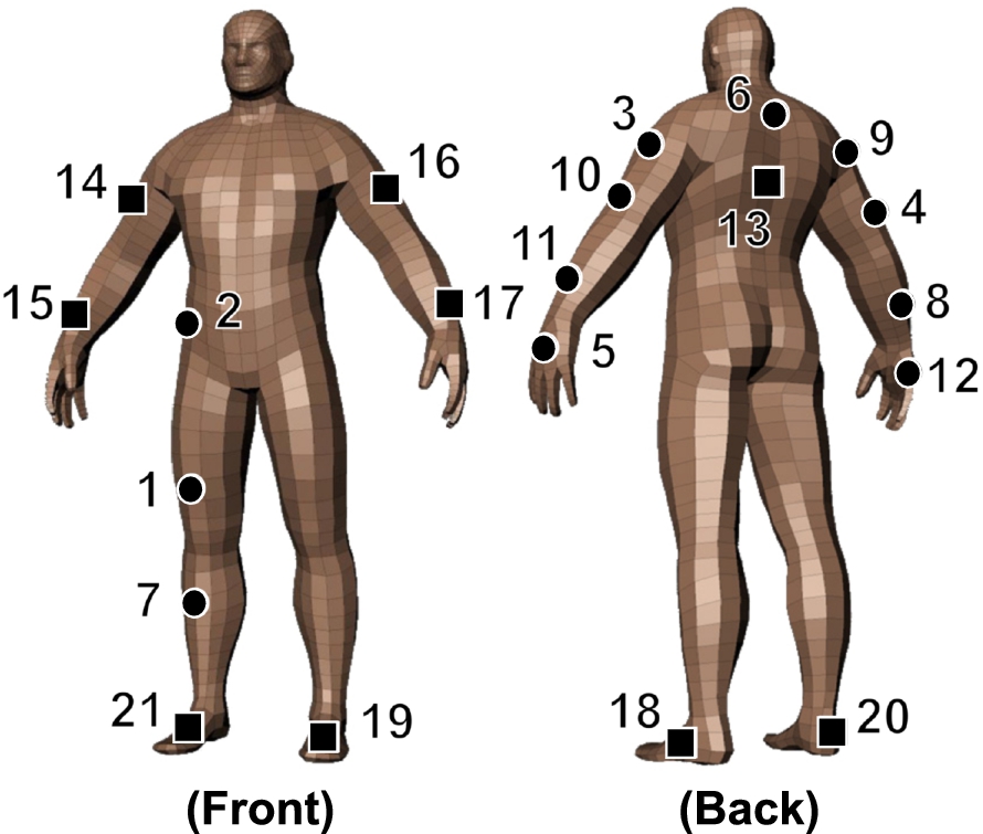
As anticipated in Section 1, the experimental data used to test our algorithm are shared data collected in the context of the European project Opportunity and provided for the so-called Opportunity Challenge [4,14,18]. Figure 1 shows the experimental configuration of the sensor nodes in the considered BSN. The output of the BSN consists of mainly accelerometric data, integrated, for some nodes, with gyroscopic and magnetometric data – in this work, in order to guarantee a low hardware complexity (and, consequently, a low cost and large battery life of the whole activity classification system), only accelerometric data will be used.1

¹
To this end, note that the cost of a gyroscope (or of a magnetometer) chip is typically at least twice that of an accelerometer chip. Similar considerations hold for power consumption requirements, as accelerometers require indeed much less power than gyroscopes and magnetometers do. This has obviously a strong impact on the battery lifetime.

For data collection, different users were asked to perform sequences of consecutive predefined movements and naturally executed daily activities. This allowed to generate highly realistic data upon which robust and flexible algorithms could be developed and trained. Data were recorded with a sampling rate

f_{samp} = 30 Hz

Fig. 1.

Opportunity Challenge setup [4,18]. The position of accelerometers (∙) and inertial measurement units (■) is highlighted.

Given a discrete set of predefined activities $A = {a_{1}, a_{2}, \dots, a_{A}}$ (with cardinality $| A | = A$ ), the metric which will be used to evaluate the performance of the proposed classification algorithm is the weighted f1 score [4], denoted as $F 1^{w}$ and evaluated as follows: $\begin{array}{rcl} F 1^{w} & = & \sum_{a = 1}^{A} 2 * (\frac{n_{a}}{N}) * F 1_{a} \\ = & \sum_{a = 1}^{A} 2 * (\frac{n_{a}}{N}) * (\frac{{prec}_{a} * {rec}_{a}}{{prec}_{a} + {rec}_{a}}) \end{array}$ where: a is the considered activity; $n_{a}$ is the number of samples of the inertial data sequence in correspondence to which a user is performing activity a; N is the total number of samples of the collected inertial data sequence; $F 1_{a}$ is the f1 score computed for activity a; and ${prec}_{a}$ and ${rec}_{a}$ are, respectively, the precision (defined as $TP / (TP + FP)$ , where TP and FP are the numbers of true positives and false positives) and the recall (defined as $TP / (TP + FN)$ , where FN is the number of false negatives) evaluated for activity a. In practice, $F 1^{w}$ is the average f1 score over all activities. Note that, beside these metrics, in the refinement step of the proposed algorithm (which is described in Section 2.2.4) two other metrics will also be considered, namely: the accuracy, defined as $(TP + TN) / (P + N)$ , where TP, TN, P, and N are, respectively, the numbers of true positives, true negatives, positives, and negatives; and the specificity, defined as $TN / (FP + TN)$ , where TN and FP are the numbers of true negatives and false positives. For reproducibility purposes, the performance of the proposed algorithm is evaluated for multiple datasets collected from different subjects. To this end, in the Opportunity dataset, for each subject, golden labels are provided, containing a single stream of (manually) labeled activities.2

Note that, while evaluating the algorithm performance, the samples containing “undefined” activities (e.g., transitions between classifiable activities), because of the temporal continuity of the collected data, are not taken into account for the evaluation of $F 1^{w}$ . For the sake of completeness, we remark that this does not mean that the algorithm is not dealing with data coming from “unknown” classes. In fact, the algorithm is not forced to always choose at least one of the considered classes and it may actually happen that for some time epoch no activities are detected at all. This will be clearer by reading the algorithm description in Section 2.2.

In the proposed algorithm, which is described in the following subsections, we will only make use of accelerometric data.

2.2. Algorithm description

Generally, an activity classification problem leads to the design of an algorithm that can estimate the sequence of occurrences of specific activities choosing from a discrete set of predefined activities $A$ , directly working on (typically) inertial signals (e.g., accelerometric and gyroscopic signals). The proposed algorithm tries to concentrate most of its complexity in a (offline) training phase, which is performed once and aims at selecting the smallest subset of nodes to extract the smallest, yet sufficient, number of accelerometric time features to guarantee a good performance (high $F 1^{w}$ ). Then, upon optimized setting of proper thresholds, the online phase is relatively light (in terms of time complexity), making real-time activity classification applications feasible.

In the following, a detailed description of the operational steps of the proposed algorithm are presented. After preliminaries on data preprocessing, the online and training phases are presented. In order to run properly, the online activity classification algorithm needs some parameters that have to be estimated and optimized during the training phase. Even though, practically, the training phase precedes the online phase, in the remainder of this subsection, after preliminaries on data processing and feature extraction, we first describe in detail, for ease of presentation, the online phase. In the training phase, the same steps of the online phase are considered, with the only difference that known (labeled) data are used to tune the key parameters of the algorithm, which are then kept constant in the (following) online phase.

2.2.1. Preliminaries on data preprocessing and feature extraction

At each node, an accelerometer outputs a stream of three-dimensional data, which corresponds to the accelerations measured by the sensor in its three reference axes. More formally, let us define the three-dimensional acceleration vector, measured at the i-th epoch, as $\begin{matrix} {\tilde{α}}_{i} = ({\tilde{α}}_{x i}, {\tilde{α}}_{y i}, {\tilde{α}}_{z i}) i \in {1, 2, \dots, N} \end{matrix}$ where N is the number of samples in the stream. For the sake of simplicity, let us assume that the accelerometer is already calibrated and, thus, ${\tilde{α}}_{xi}$ , ${\tilde{α}}_{yi}$ , and ${\tilde{α}}_{zi}$ are expressed in g units. Furthermore, the accelerometric data are low-pass filtered in order to deal with smoother data in both training and online phases. To this end, the recursive low-pass filtering used for each accelerometric data stream is the same used in [7] and characterized by the following equation: $\begin{matrix} (1) & y_{i} = \{\begin{matrix} x_{1} & i = 1 \\ 0.8 \cdot y_{i - 1} + 0.1 \cdot (x_{i} + x_{i - 1}) & 2 ⩽ i ⩽ N \end{matrix} \end{matrix}$ where $x_{i}$ is the i-th sample of the data stream ( $x \in {{\tilde{α}}_{x}, {\tilde{α}}_{y}, {\tilde{α}}_{z}}$ ), $y_{i}$ is the i-th sample of the filtered data stream ( $y \in {α_{x}, α_{y}, α_{z}}$ ). The cut-off frequency $f_{co}$ of the low-pass filter defined in (1) is $f_{co} \approx \frac{f_{samp}}{30} = 1 Hz$ . Therefore, we denote the filtered signal as $\begin{matrix} α_{i} = (α_{xi}, α_{yi}, α_{zi}) i \in {1, 2, \dots, N} \end{matrix}$ and the norm of $α_{i}$ as $\begin{matrix} {\overline{α}}_{i} = | α_{i} | = \sqrt{α_{xi}^{2} + α_{yi}^{2} + α_{zi}^{2}} i \in {1, 2, \dots, N} . \end{matrix}$

Starting from the filtered signal, at the i-th epoch, two types of simple features are of interest and can be extracted. The first one, denoted as p-feature (where “p” stands for “parallel”) and indicated with ${acc}_{i}^{(p)}$ , is a properly chosen component of the normalized3

³
Note that, by normalizing the acceleration vector (for the p-feature), we are implicitly assuming that no linear acceleration is present (i.e., the device is still) and only the gravity acceleration contribution (i.e., 1 g) is measured by the accelerometer. Note that, although this assumption is not always true, in the majority of human movements it is true that the magnitude of the linear acceleration is rather lower than that of the gravity component.

(to unity) acceleration vector, i.e.,

{acc}_{i}^{(p)} \in {α_{xi} / | α_{i} |, α_{yi} / | α_{i} |, α_{zi} / | α_{i} |}

. In particular, the chosen component is the one parallel to the “main” axis of the related body segment. For instance, considering Fig. 1: for node 1,

{acc}_{i}^{(p)}

is the acceleration value measured along the femur direction; for node 7, the one measured along the tibia. Observe that, due to the normalization,

{acc}_{i}^{(p)}

can only assume real values in

[- 1, + 1]

The second considered feature, denoted as dev-feature and indicated with $σ_{i} (s)$ , is the standard deviation of the norm of the acceleration computed on a sliding window (with fixed length $L = 2 \cdot s + 1$ and centered at the i-th sample4

⁴

More details about the definition of the window, especially at the borders of the acceleration signal, are given in [8].

) that runs over all the acceleration samples. Neglecting border effects (the extension is straightforward, as shown in [8]),

σ_{i} (s)

can be expressed as follows:

\begin{matrix} (2) & σ_{i} (s) = \sqrt{\frac{\sum_{k = i - s}^{i + s} {[{\overline{α}}_{k} - μ_{k} (s)]}^{2}}{L - 1}} \end{matrix}

where

\begin{matrix} (3) & μ_{k} (s) ≜ \frac{\sum_{k = i - s}^{i + s} {\overline{α}}_{k}}{L - 1} . \end{matrix}

It can be observed that

σ_{i} (s)

is always larger than or equal to 0 – typically, it is not considerably larger than 1 (due to the expression of the accelerometric data in g units). While evaluating the classification performance of the proposed algorithm, s is set to 7 samples and, therefore, the dev-features are computed on a window of length

L = 15

samples (i.e., 0.5 s).

2.2.2. The general idea

Considering a single activity $a \in A$ , the output of an activity classification algorithm is given by a binary sequence $w (a) = (w_{1} (a), w_{2} (a), \dots, w_{N} (a))$ where $w_{i} (a) = 0$ if a is not detected at epoch i (the index i runs over the samples of the collected accelerometric data sequence) or $w_{i} (a) = 1$ if a is detected. In particular, $w (a)$ contains “activity windows” (disjoint groups of consecutive “1”s), within which the activity a has been detected. The length of each activity window is recursively determined – using three parameters $ℓ_{1}$ , $ℓ_{2}$ , and $ℓ_{3}$ , optimized independently for each activity. This process will be described later.

For each considered activity, the proposed activity classification algorithm aims at automatically selecting the best nodes in the BSN and the corresponding most significant feature types, that can best discriminate the occurrence of the considered activity (e.g., the thigh node is intuitively one of the best nodes to estimate a “sit” activity, whereas the feet nodes give relevant information about the “walk” activity). More formally, let us define as $F = {f_{1}, f_{2}, \dots, f_{F}}$ (with cardinality $| F | = F$ ) a set of features where the generic feature $f \in F$ corresponds to a feature “type” (p-feature or dev-feature) associated with a specific node. As an example, referring to Fig. 1, $f = 1 p$ is the p-feature extracted from the thigh node (i.e., node 1) and $f = 7 d$ is the dev-feature extracted from the tibia node (i.e., node 7). In the following, when referring to the value of a feature, we will implicitly refer to the value of the “embedded” feature type. Furthermore, given a specific activity a, $C_{a}^{*} \subset F$ represents the subset of the most significant features used to classify activity a.5

⁵
Note that, throughout this paper, the term “optimal” and the superscript “*” are equivalently used with reference to the tunable parameters considered in the proposed algorithm. Furthermore, if not stated otherwise, the optimality is always intended in terms of classification performance through the f1 score (when activities are independently considered) and the weighted f1 score (when activities are combined together).

The proposed algorithm identifies activities by properly thresholding the selected features. In particular, referring to a given feature f, an activity a is considered as detected at the samples in correspondence to which the feature (type) is between the (lower and upper) thresholds $t_{1} (a, f)$ and $t_{2} (a, f)$ , which are specifically derived and optimized independently for each activity a and for each feature f. The optimal values ${t_{1}^{*} (a, f)}_{a \in A, f \in C_{a}^{*}}$ and ${t_{2}^{*} (a, f)}_{a \in A, f \in C_{a}^{*}}$ are determined in the training phase, as will be described later.

In order for the activity classification algorithm to output a single sequence $w = (w_{1}, w_{2}, \dots, w_{N})$ (where $w_{i} = 0$ if no activities are detected and $w_{i} = a$ if activity a is detected, i.e., $w_{i} (a) = 1$ ), since $w_{i} (a_{j}) = w_{i} (a_{k}) = 1$ may happen for some $i \in {1, 2, \dots, N}$ and for some $j \neq k$ , with $j, k \in {1, 2, \dots, A}$ , different priorities need to be assigned to the activities. The priorities are denoted as $q = (q (a_{1}), q (a_{2}), \dots, q (a_{A}))$ , where each element (which indicates the priority of each considered activity) can assume real values in $[0, 1]$ . The priorities’ list $q$ must be interpreted as follows: if $q (a_{i}) > q (a_{j})$ , with $i, j \in {1, 2, \dots, A}$ , activity $a_{i}$ has a higher priority than activity $a_{j}$ . The priority assigned to an activity is strongly related to the confidence in correctly detecting that activity and is based on the evaluation of specific performance metrics, which are evaluated in the training phase, as will be described later. In this way, the output sequence $w$ is an $(A + 1)$ -ary sequence of activity labels, where the label of the activity with highest priority is selected in the cases where more than one activity is detected at the same epoch. The optimal priorities’ list $q^{*}$ is determined in the training phase, as described later.

2.2.3. Activity classification

The online phase of the proposed algorithm is based on three main steps: (i) a first coarse classification step; (ii) a refinement step; (iii) and a final priority-based activity combination step.

Concerning the first coarse classification step, which is executed independently for each activity to be classified, a specific activity a is detected at epoch i (i.e., $w_{i} (a) = 1$ ) if all the features belonging to $C_{a}^{*}$ are comprised between the corresponding optimal thresholds ${t_{1}^{*} (a, f)}_{f \in C_{a}^{*}}$ and ${t_{2}^{*} (a, f)}_{f \in C_{a}^{*}}$ .

In the first coarse classification step, a single occurrence of an activity can be missed (because of little pauses or random movements). This can be avoided, or at least mitigated, by applying to the detected activity windows a refinement step which takes into account the length of the estimated activity windows. More specifically, given a specific activity a, in our implementation the refinement step is based on the following sequential operations: (1) every “null window” (a group of consecutive “0”s), with a length (in terms of number of samples) shorter than $ℓ_{1}^{*}$ , is switched to an activity window (and incorporated in the preceding and following activity windows, which are then fused together); (2) every activity window with a length shorter than $ℓ_{2}^{*}$ is turned into a null window; (3) step 1 is repeated considering now every null window with a length shorter than $ℓ_{3}^{*}$ .

Finally, the priority-based activity combination step consists in combining the sequences $w (a_{1})$ , $w (a_{2}), \dots$ , and $w (a_{A})$ into a single sequence $w$ of activity labels, on the basis of the optimal priorities $q^{*}$ assigned to the activities.

2.2.4. Algorithm training

In order to work effectively, the proposed algorithm needs to be properly trained by exploiting the part of collected data for which the occurrences of the activity of interest are correctly (manually) labeled. The training phase aims at estimating the optimal values of the key parameters that will be used in the online phase. In particular, for each activity a the following parameters need to be estimated: (i) the optimal subset of features $C_{a}^{*}$ , along with the corresponding optimal thresholds ${t_{1}^{*} (a, f)}_{f \in C_{a}^{*}}$ and ${t_{2}^{*} (a, f)}_{f \in C_{a}^{*}}$ ; (ii) the optimal thresholds $ℓ_{1}^{*}$ , $ℓ_{2}^{*}$ , and $ℓ_{3}^{*}$ , used to refine the estimated activity windows; (iii) the optimal activities’ priorities list $q^{*}$ , over all activities.

A detailed flow diagram of the implementation steps of the training phase of the proposed algorithm is shown in Figs 2, 3, and 4 and will be now described, distinguishing between its three component blocks (the same of the online phase): (i) the first coarse classification step; (ii) the refinement step; and (iii) the final priority-based activity combination step.

Fig. 2.

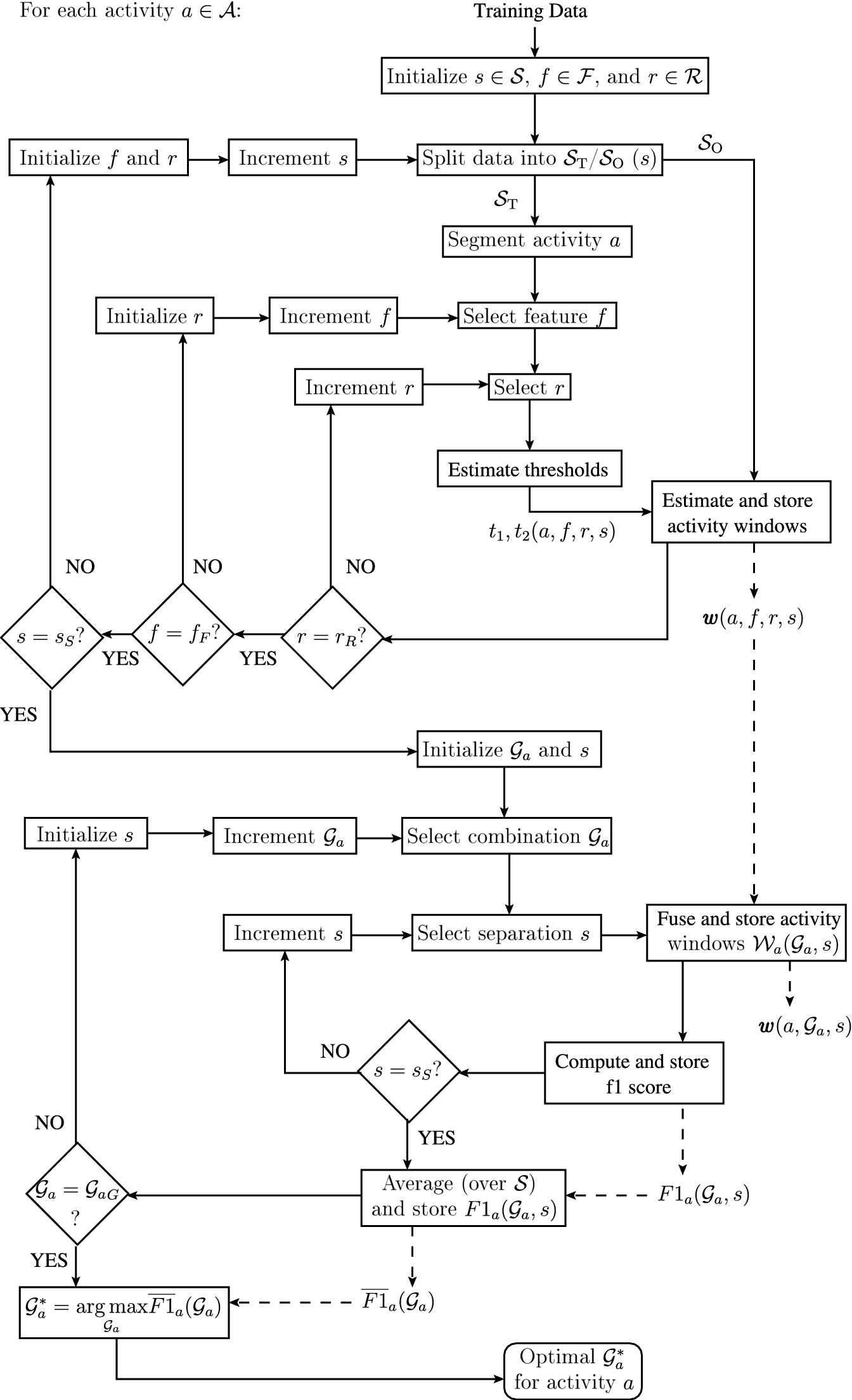
Detailed flow diagram of the implementation steps of the proposed algorithm’s training phase: the first coarse classification step.

Fig. 3.

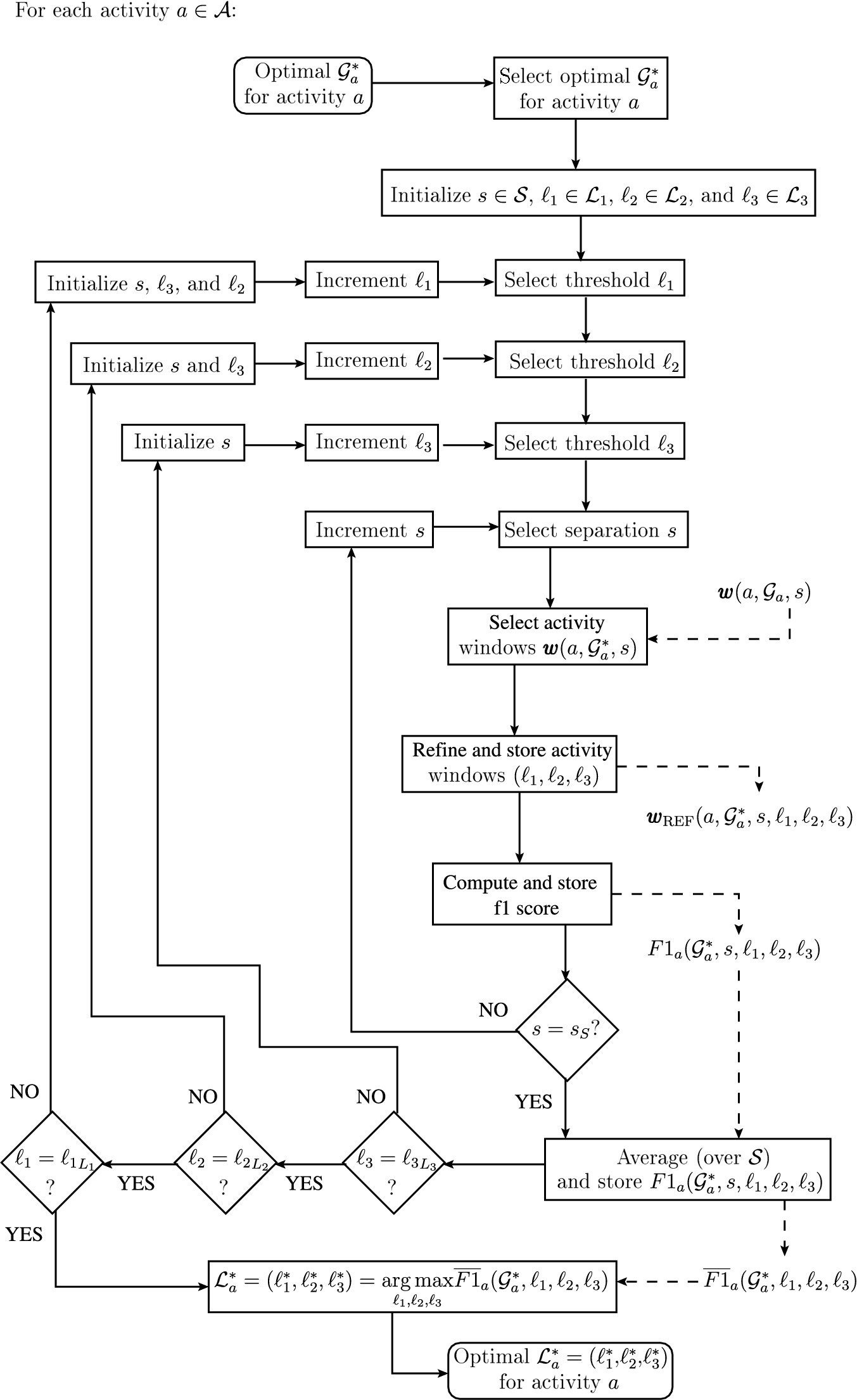
Detailed flow diagram of the implementation steps of the proposed algorithm’s training phase: the refinement step.

Fig. 4.

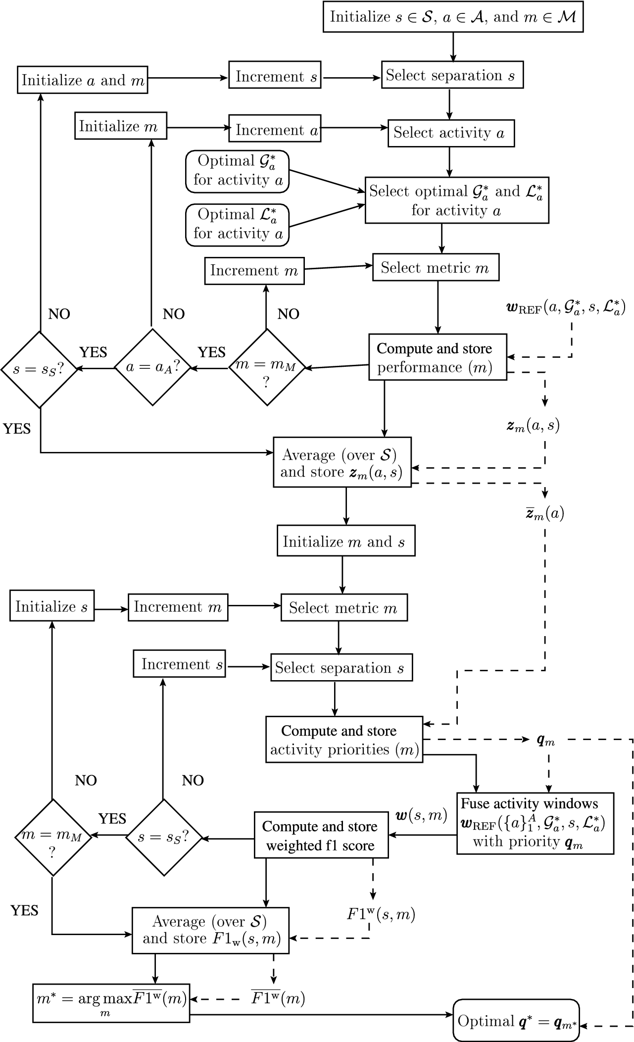
Detailed flow diagram of the implementation steps of the proposed algorithm’s training phase: the final priority-based activity combination step.

Coarse classification At the beginning of the coarse classification step, shown in Fig. 2 and executed for each activity a, the set $F = {f_{1}, f_{2}, \dots, f_{F}}$ , whose elements are all the initial features, must be (manually) defined. Similarly, the set $S$ (with cardinality $| S | = S$ ) accounts for different ways (each way is identified by a partition $s = (S_{T} / S_{O})$ ) of separating the (training) dataset into the two subsets $S_{T}$ and $S_{O}$ (s will be denoted as “separation”). Finally, $R$ (with cardinality $| R | = R$ ) accounts for possible values of “confidence,” which will be given in terms of a given percentage of the Probability Mass Function (PMF) characterizing the values of the selected feature for the activity of interest, considered to derive the thresholds ${t_{1} (a, f)}_{a \in A, f \in F}$ and ${t_{2} (a, f)}_{a \in A, f \in F}$ – more details about confidence are provided below with an example. Note that the separation into the two subsets $S_{T}$ and $S_{O}$ is done in order to cross-validate the statistical performance of the algorithm, i.e., to assess how the algorithm’s performance will generalize with an independent dataset. In the machine learning field, this is a common practice used to derive unbiased performance of an algorithm, especially when only training data are available [5].

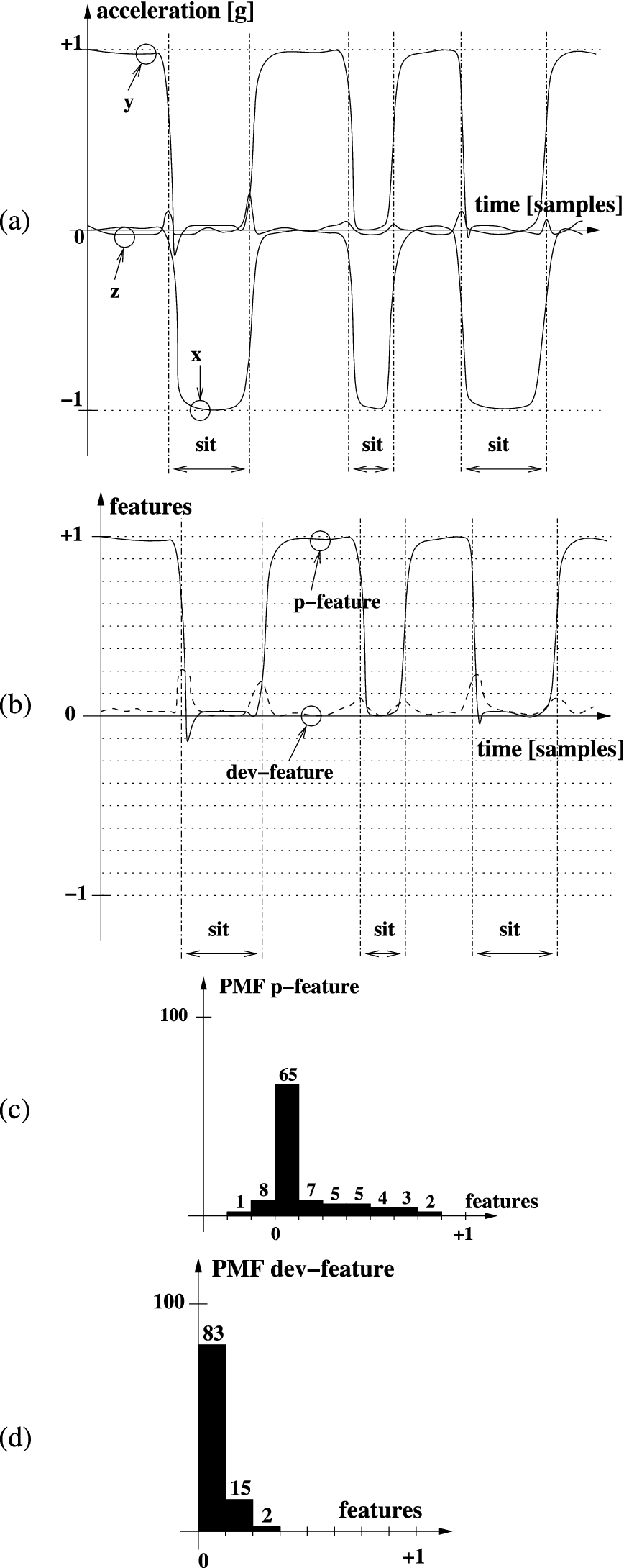
The goal of the first part of the coarse classification step is to estimate and store the activity windows ${w (a, f, r, s)}_{a \in A, f \in F, r \in R, s \in S}$ . As already explained in Section 2.2.3, the activity windows are derived, for a given activity a, by applying to each feature $f \in F$ (considering the dataset $S_{O}$ associated with the selected s) the (properly estimated) thresholds $t_{1} (a, f, r, s)$ and $t_{2} (a, f, r, s)$ – unlike in the online phase, $t_{1}$ and $t_{2}$ depend not only on a and f, but also on s (as, obviously, the thresholds depend on the used data-set) and r (as the “width” between the thresholds depend on the desired confidence – the larger, the higher the required confidence).

Fig. 5.

Description of the thresholds estimation step, which appears in Fig. 2, for an illustrative acceleration signal produced at the thigh node: (a) acceleration signal (the x, y, and z components are highlighted); (b) p-feature (straight line) and dev-feature (dashed line) extracted from the previous acceleration signal; PMFs of (c) p-feature and (d) dev-feature evaluated in the “sit” intervals.

In order to clarify the process which leads to the identification of the thresholds for activity classification, we consider an example relative to the acceleration signals produced at the thigh node (i.e., node 1 in Fig. 1) and used to detect the “sit” activity. An illustrative description of the thresholds estimation step is shown in Fig. 5: the p-feature (i.e., $f = 1 p$ ) and the dev-feature (i.e., $f = 1 d$ ), shown in Fig. 5(b), are first extracted from the acceleration signals (shown in Fig. 5(a), in the x, y, and z axes) and evaluated discretely in the “sit” intervals (assuming that $a = sit$ and for a given $s \in S$ ) in order to obtain their PMFs in such intervals (the PMFs of the p-feature and the dev-feature are shown in Figs 5(c) and 5(d), respectively). Given a, f, s, for each value of $r \in R$ , the thresholds $t_{1} (a, f, r, s)$ and $t_{2} (a, f, r, s)$ are then chosen as the extremes of the shortest interval $(t_{1}, t_{2})$ which comprises at least r% of the probability mass.

The second part of the coarse classification step, still performed independently for each $a \in A$ , is based on the fusion of different combinations of the previously stored activity windows ${w (a, f, r, s)}_{f \in F, r \in R, s \in S}$ . The goal is to find, for each activity, the optimal combination $G_{a}^{*}$ (among the G possible combinations), where the generic combination $G_{a}$ is associated with a possible subset of features $C_{a} \subset F$ and two values of r, i.e., $r_{p}$ and $r_{dev}$ , from which the thresholds $t_{1} (a, f, r, s)$ and $t_{2} (a, f, r, s)$ can be estimated when the considered f is, respectively, a p-feature or a dev-feature. An example, a possible instance of $G_{a}$ could be $(C_{a} = {1 d, 1 p, 4 p}, r_{p} = 93 %, r_{dev} = 97 %)$ .

Given a combination $G_{a}$ and a separation $s \in S$ , the set $W_{a} (G_{a}, s)$ is defined as the subset of ${w (a, f, r, s)}_{f \in F, r \in R}$ with $(f, r) \in G_{a}$ . The sequences of activity windows in $W_{a} (G_{a}, s)$ are then fused together (and stored for future use) into a single sequence of activity windows $w (a, G_{a}, s)$ , obtained from the “logical AND” of all the considered sequences of activity window. The f1 score of $w (a, G_{a}, s)$ , denoted as $F 1_{a} (G_{a}, s)$ , is then computed and stored. By averaging ${F 1_{a} (G_{a}, s)}_{s \in S}$ over all possible separations in $S$ and denoting this average as ${\overline{F 1}}_{a} (G_{a}) = \sum_{s \in S} F 1_{a} (G_{a}, s) / S$ , the optimal $G_{a}^{*}$ is selected as follows: $\begin{matrix} (4) & G_{a}^{*} = \underset{G_{a}}{arg max} {\overline{F 1}}_{a} (G_{a}) . \end{matrix}$

Refinement The next refinement step, shown in Fig. 3 and executed for each activity a, retraces the operations of the previous step in order to estimate the optimal thresholds $L_{a}^{*} = (ℓ_{1}^{*}, ℓ_{2}^{*}, ℓ_{3}^{*})$ used to refine the previously estimated activity windows, but considering now just the optimal combination $G_{a}^{*}$ . To this end, three sets $L_{1} \subset N$ , $L_{2} \subset N$ , $L_{3} \subset N$ are defined.6

⁶

These values should be properly chosen in the order of at most a few seconds in order to filter out just the windows of samples which correspond to little pauses or random movements.

Given a separation

s \in S

, all possible combinations of

ℓ_{1} \in L_{1}

ℓ_{2} \in L_{2}

, and

ℓ_{3} \in L_{3}

are used to refine the previously estimated sequence of activity windows

w (a, G_{a}^{*}, s)

as already described in Section 2.2.3. For every considered combination of

ℓ_{1} \in L_{1}

ℓ_{2} \in L_{2}

, and

ℓ_{3} \in L_{3}

, the refined sequences of activity windows

{w_{REF} (a, G_{a}^{*}, s, ℓ_{1}, ℓ_{2}, ℓ_{3})}_{s \in S}

are then stored (for future use) and their f1 scores

{F 1_{a} (G_{a}^{*}, s, ℓ_{1}, ℓ_{2}, ℓ_{3})}_{s \in S}

are computed and stored. By averaging

{F 1_{a} (G_{a}^{*}, s, ℓ_{1}, ℓ_{2}, ℓ_{3})}_{s \in S}

over all possible separations in

S

and denoting this average as

{\overline{F 1}}_{a} (G_{a}^{*}, ℓ_{1}, ℓ_{2}, ℓ_{3}) = \sum_{s \in S} F 1_{a} (G_{a}^{*}, s, ℓ_{1}, ℓ_{2}, ℓ_{3}) / S

, the optimal thresholds

L_{a}^{*}

are selected as follows:

\begin{matrix} (5) & L_{a}^{*} = (ℓ_{1}^{*}, ℓ_{2}^{*}, ℓ_{3}^{*}) = \underset{(ℓ_{1}, ℓ_{2}, ℓ_{3})}{arg max} {\overline{F 1}}_{a} (G_{a}^{*}, ℓ_{1}, ℓ_{2}, ℓ_{3}) . \end{matrix}

Priority-based activity combination During the final step, shown in Fig. 4, the optimal list of activities’ priorities $q^{*}$ is estimated. To this end, a set of performance metrics $M = {m_{1}, m_{2}, \dots, m_{M}}$ (where $| M | = M$ ) is considered. Specifically, in this work we consider the following performance metrics (defined as in Section 2.1): (i) f1 score, (ii) precision, (iii) recall, (iv) specificity, and (v) accuracy. First, given an activity a and a separation s, every performance metric $m \in M$ is used to evaluate the performance associated with the sequence of activity windows $w_{REF} (a, G_{a}^{*}, s, L_{a}^{*})$ and the corresponding value $z_{m} (a, s)$ is stored. For given activity a and metric m, the obtained values ${z_{m} (a, s)}_{s \in S}$ are then properly averaged over all possible separations $s \in S$ and the resulting ${\overline{z}}_{m} (a) = \sum_{s \in S} z_{m} (a, s) / S$ is used to compose (and store) a priority-based list of activities $q_{m} = (q_{m} (a_{1}), q_{m} (a_{2}), \dots, q_{m} (a_{A})) ≜ ({\overline{z}}_{m} (a_{1}), \dots, {\overline{z}}_{m} (a_{A}))$ . Specifically, the priorities’ lists ${q_{m}}_{m \in M}$ defines the priorities assigned to every activity according to the specific performance metric m.

At this point, for given $s \in S$ and $m \in M$ , the A sequences of activity windows ${w_{REF} (a, G_{a}^{*}, s, L_{a}^{*})}_{a \in A}$ are combined together, on the basis of the priorities’ list $q_{m}$ , resulting in a single sequence of activity windows $w (s, m)$ and the corresponding weighted f1 score, denoted as $F 1^{w} (s, m)$ , is computed and stored. By averaging ${F 1^{w} (s, m)}_{s \in S}$ over all possible separations in $S$ and denoting this average as $\overline{F 1^{w}} (m) = \sum_{s \in S} F 1^{w} (s, m) / S$ , the optimal $q^{*} = (q^{*} (a_{1}), q^{*} (a_{2}), \dots, q^{*} (a_{A}))$ is then estimated as the list $q_{m}^{*}$ where the metric $m^{*}$ is selected as follows: $\begin{matrix} (6) & m^{*} = \underset{m}{arg max} \overline{F 1^{w}} (m) . \end{matrix}$

At the end of the training phase, for each activity a, the optimal $G_{a}^{*}$ is used to further estimate the optimal thresholds ${t_{1}^{*} (a, f)}_{f \in C_{a}^{*}}$ and ${t_{2}^{*} (a, f)}_{f \in C_{a}^{*}}$ , which will be actually used in the online phase, with the only difference that the entire training dataset is now considered to derive them. Therefore, for each activity a, the following optimal parameters have to be stored for future use in the online phase: $C_{a}^{*}$ ; ${t_{1}^{*} (a, f)}_{f \in C_{a}^{*}}$ and ${t_{2}^{*} (a, f)}_{f \in C_{a}^{*}}$ ; $L_{a}^{*} = (ℓ_{1}^{*}, ℓ_{2}^{*}, ℓ_{3}^{*})$ . Finally, the optimal list of priorities $q^{*} = (q^{*} (a_{1}), q^{*} (a_{2}), \dots, q^{*} (a_{A}))$ , over all possible activities, is also stored.

3. Results and discussion

The performance of the proposed algorithm has been evaluated for the classification of activities related to modes of user locomotion. In particular, $A = 4$ activities are considered: stand, walk, sit, and lie (i.e., $A = {stand, walk, sit, lie}$ ). In Section 3.1, we outline the considered configurations of nodes and features for the proposed algorithm and the following existing classification algorithms (as anticipated in Section 1): the k-NN (with $k = 1$ and $k = 3$ ), the NCC, the LDA, and the QDA – more details about their practical implementation are given in [4,5,12]. All the algorithms (for all possible configurations) are tested on the same dataset, which, for the purpose of repeatability, takes into account four different subjects [14]. In all cases, $R = {90, 91, 92, \dots, 100}$ , $L_{1} = {0, 1, 2, \dots, 60}$ , $L_{2} = {0, 5, 10, \dots, 200}$ , $L_{3} = {0, 5, 10, \dots, 200}$ , $M = {f 1 score, precision, recall, specificity, accuracy}$ , and $S = 4$ different separations of the training dataset are considered. The obtained classification performance results are presented in Section 3.2. In Section 3.3, the time complexity of all considered algorithms is summarized. Finally, in Section 3.4 the robustness of the proposed algorithm against rotational noise is investigated, as this is particularly meaningful for BSN-based activity classification applications.

3.1. Configurations of nodes and features

Overall, we consider 38 different configurations of nodes (and feature types): configurations 1–31 (with at most 7 nodes) apply to the proposed algorithms and the four considered existing classification algorithms (k-NN, NCC, LDA, and QDA) and rely on the use of accelerometric data; configurations 32–38 (with more than 7 nodes) apply only to the four considered existing classification algorithms and rely on the use of other (besides accelerometers) inertial sensors (e.g., magnetometers). Each configuration involves a specific nodes’ configuration, explicitly shown in the x axis of Fig. 6 (which will be described in the next subsection) with reference to the node number in Fig. 1.

Note that, given a set of activities that need to be classified, the number and placement of the devices could be preliminary devised and used by determining which devices may provide the most different signal patterns in correspondence to different activities. However, in this work we take advantage of the fact that an exhaustive dataset was provided in the Opportunity Challenge [4,14,18], since the BSN used to acquire the given dataset was composed by a large number of sensor devices placed all over the users’ body. The automatic selection of the best devices and features is then left to the “artificial intelligence” of the algorithm (specifically, during the training phase). In this way, some sensor devices, which could have appeared to be intuitively useless at classifying some activities, may be instead selected as good candidates. Furthermore, once the best set of devices is determined, the proposed approach also allows to automatically determine the best subset of devices and features for each activity that has to be classified and such subset may likely change from activity to activity.

Fig. 6.

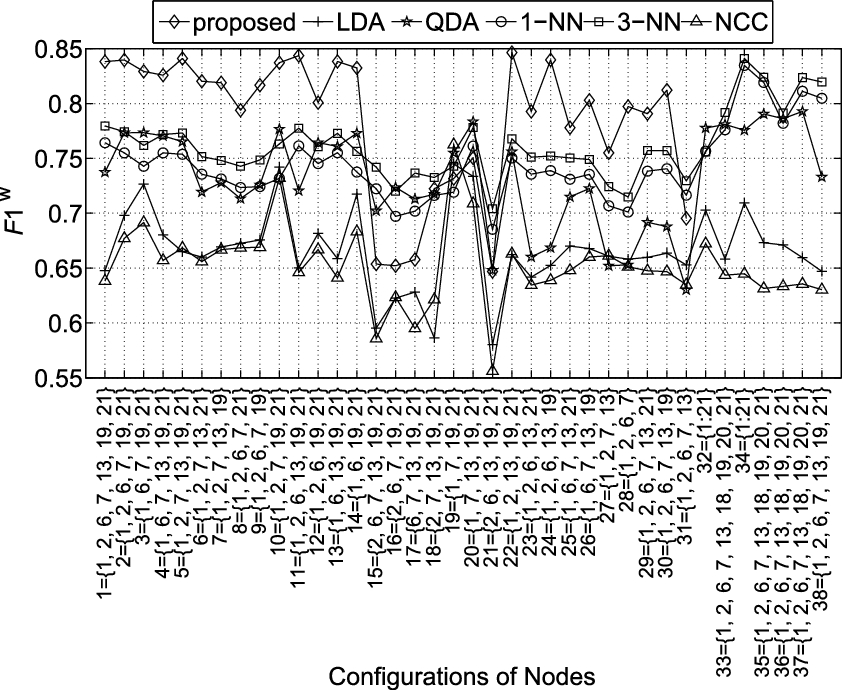
Average (over 4 subjects) classification performance (i.e., weighted f1 score) as a function of the considered configurations of nodes. The performance of the proposed algorithm is compared with that of some existing algorithms, averaging the performance of the four considered subjects. For every configuration, the considered subsets of BSN nodes (numbered as in Fig. 1) are highlighted. The features per configuration and per algorithm are properly selected as summarized in Section 3.1.

Fig. 7.

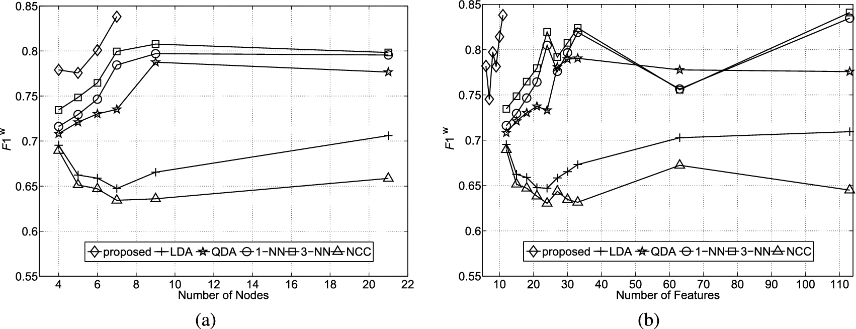
Average (over 4 subjects) classification performance (i.e., weighted f1 score) as a function of the considered (a) number of nodes and (b) number of features. For each considered algorithm, the configurations which use the same number of (a) nodes or (b) features have been averaged together.

The choice of the nodes’ feature types for each classification algorithm can be summarized as follows.

Configurations 1–31; proposed algorithm. Only p-features and dev-features are considered. Specifically: for nodes 7, 1, 2, and 6 (namely, the nodes of the main vertical segment of the human body) both types of features are extracted; for nodes 13, 19, and 21 (feet nodes and a second node for the back) only the d-feature is extracted. In particular, at most $F = 11$ features are considered (for instance, the set of features of Configuration 1 is $F = {1 p, 2 p, 6 p, 7 p, 1 d, 2 d, 6 d, 7 d, 13 d, 19 d, 21 d}$ ).

Configurations 1–31; k-NN, NCC, LDA, and QDA algorithms. For all the nodes, the mean of every acceleration component within a sliding window is considered, leading to 3 features extracted at each node. Therefore, at most $F = 21$ features are considered.

Configurations 32–38; k-NN, NCC, LDA, and QDA algorithms. For all the nodes, the mean of every acceleration component within a sliding window is still considered (as in the previous case). In addition, for configurations from 34 to 38, the mean within a sliding window is also computed for the 3 components of the gyroscope and magnetometer signals, or some combinations of them, as summarized below:

for configuration 34: every node equipped with gyroscope and magnetometer (i.e., nodes from 13 to 21) produces 6 additional features (3 from gyroscope and 3 from magnetometer);

for configuration 35: 6 additional features (3 from gyroscope and 3 from magnetometer) are extracted at node 13;

for configuration 36: 3 additional gyroscopic features are extracted at node 13;

for configurations 37 and 38: 3 additional magnetometric features are extracted at node 13.

3.2. Classification performance

The performance of the proposed algorithm has been evaluated for 31 different configurations of nodes in order to determine the optimal subset of BSN nodes (and, thus, of features) useful for the activity classification. In particular, in Fig. 6, the performance of our algorithm (in terms of $F 1^{w}$ ) is shown as a function of the configurations of nodes, averaging over the considered four subjects. A comparison with the performance obtained with the other considered algorithms, run with the same configurations of nodes, is also shown. Note that the performance of these algorithms is also evaluated for more complex configurations of nodes (for a total of 38 configurations), which consider the use of a larger number of nodes and features. It is easy to observe that, in most of the considered configurations of nodes, our algorithm outperforms the other ones. It can also be seen that some of the reference algorithms (in particular, k-NN and QDA) have similar performance to ours, but only when considering, in their cases, more complex configurations with larger numbers of nodes and features. Note also that the central “hole” in Fig. 1 is associated with those configurations of nodes (namely, 15, 16, 17, 18, and 21 in Fig. 6) which do not use node 1 (the thigh node) in Fig. 1, i.e., a key node in discriminating between sit and stand activities. A similar observation can be made for configuration 31 (as denoted in Fig. 6), which hardly discriminates between stand and walk due to the absence of both feet nodes (namely, nodes 19 and 21 in Fig. 1).

In order to better investigate the impact of the number of nodes on the performance of the considered algorithms, in Fig. 7(a) the performance of the considered algorithms is properly averaged over all configurations with the same number of nodes. It can be observed that, for a given number of nodes in the BSN, our algorithm, making use of configurations with at most 7 nodes, outperforms the others. Moreover, with only 7 nodes, our algorithm outperforms all existing algorithms, including the k-NN and QDA, run with a much larger number of nodes (e.g., 21).

Another aspect to take into account is the number of features used in the algorithms. Unlike the existing algorithms, where each node generates at least three features,7

⁷
The typical features computed at each node are the mean of every acceleration component within a sliding window. In addition, other six features are considered for nodes provided with gyroscopes and magnetometers. A standard deviation-related feature has been also used giving however poor performance.

our algorithm is such that a maximum of two features (i.e., the p-feature and the dev-feature) can be extracted at each node. In Fig. 7(b), it is then shown how the algorithms’ performance changes with respect to the considered overall number of features (over all nodes). It can be concluded that our algorithm provides the same, or even better, performance, with respect to the other algorithms, using a significantly smaller number of features. The number of used features has a significant impact on the time complexity of a classification algorithm, as it will be explained in Section 3.3, allowing a better real-time applicability of our algorithm with respect to the others. As previously observed, k-NN and QDA are the only algorithms which can achieve, for a very large number of features (over 110), a performance similar to that of our algorithm (using only 11 features).

For the sake of completeness, we want to highlight that, if the previously cited configurations 15, 16, 17, 18, 21 in Fig. 6 (which do not use node 1 in Fig. 1) are not taken into account for the evaluation of the curves in Fig. 7, the performance of our algorithm improves significantly more (in relative terms) than those of the other algorithms.

Finally, on the basis of the previous results, configuration 22 (as denoted in Fig. 6) can be identified as the best configuration of nodes for our algorithm. In particular, it needs 5 nodes (namely, nodes {1, 2, 13, 19, 21} in Fig. 1) and generates $F = 7$ features (5 dev-features, one per node, and 2 p-features, associated with nodes 1 and 2 in Fig. 1). Using this configuration, our algorithm obtains a value of $F 1^{w}$ around 85%. The second best algorithm, i.e., the k-NN (with $k = 3$ ), reaches a value of $F 1^{w}$ around 77% using 15 features (more than twice the number in our algorithm) and more sensors (indeed, gyroscopes and magnetometers are available in nodes {13, 19, 21} in Fig. 1). Furthermore, the best among the other algorithms (again, the k-NN with $k = 3$ ) obtains its highest $F 1^{w}$ score (namely, $F 1^{w} = 84$ %) using a significantly more complex configuration (namely, configuration 34 in Fig. 6), which comprises a total of 21 nodes and $F = 113$ features.

3.3. Time complexity

The time complexity of the proposed algorithm has been evaluated and compared with those of the classification algorithms previously considered for performance comparison.8

⁸
Recall that, we here consider the time complexity of the online phase due to its impact on real-time applicability of the algorithm and due to the fact that the training phase should be performed just once (offline), provided that the BSN configuration does not change over time.

In particular, it is possible to prove that the time complexity of the online phase of our algorithm is a linear function of the number of features F and the number of activities A. In Table 1, the time complexity of our algorithm is reported along with those of the other considered algorithms [5,12]. It can be observed that the time complexity of all algorithms is a linear function of the number of features F. In addition, our algorithm, the NCC, LDA, and QDA algorithms have a complexity linearly dependent on the number of activities A, but independent of the training dataset size D, whereas the time complexity of the k-NN algorithm depends linearly on D and is independent of A. Two considerations can now be made about A, D, and F:

the number of activities is typically quite larger than the size of the training dataset (i.e., $A ≪ D$ );

the classification performance of the proposed algorithm, when considering a few features (i.e., for small values of F), is far better than those of the NCC, the LDA, and the QDA algorithms (and also slightly better than that of the k-NN algorithm).

For these reasons, it can be concluded that our algorithm (i) guarantees the best compromise between classification performance and time complexity and (ii) outperforms, for a given number of features, the other algorithms.

Table 1

Time complexity of the online phase for the considered algorithms

Algorithm	Time Complexity
proposed, NCC, LDA, and QDA	$O (F \cdot A)$
k-NN	$O (F \cdot D)$

Fig. 8.

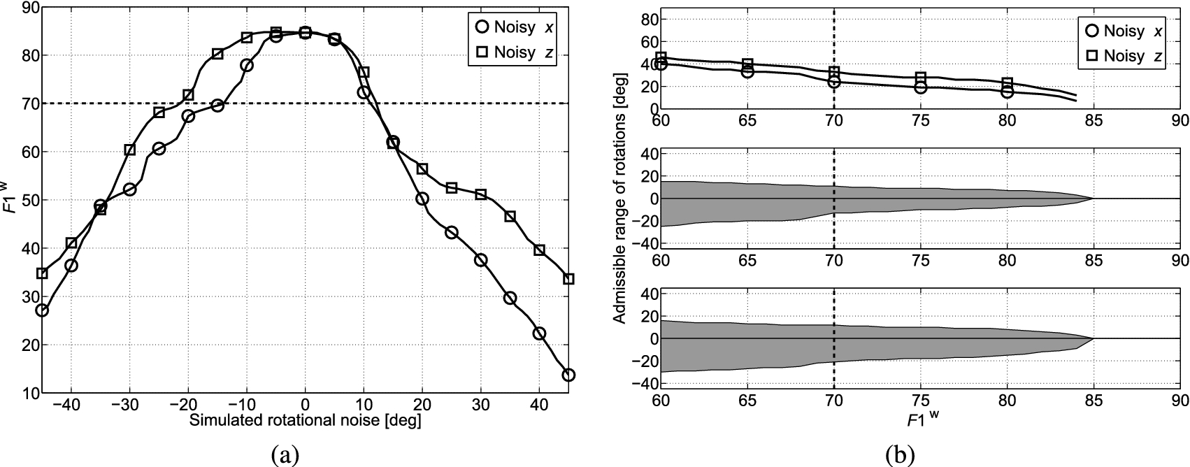
Average (over 4 subjects) classification performance (i.e., weighted f1 score) of the proposed algorithm in the presence of simulated rotational noise: (a) the weighted f1 score as a function of the intensity of the simulated rotational noise; (b) the admissible range of rotations as a function of the weighted f1 score. The previously estimated optimal configuration of nodes (i.e., configuration 22, as denoted in Fig. 6) is considered. Indicative thresholds (dashed lines), corresponding to an admissible minimum performance of $F 1^{w} = 70$ %, are also shown in two subfigures.

3.4. Robustness to noise of the proposed algorithm

A typical problem of a real BSN scenario consists of unwanted rotations in the displacement of the BSN nodes, that can differ between the training and the online phases. It is then of interest to investigate the robustness of BSN-based activity classification algorithm to rotational noise. To this end, artificial rotational noise has been added to the accelerometric data, simulating possible rotations of a device around its three reference axes. We remark that modeling rotations around the accelerometer axes, rather than around the body axes, is just an assumption, which is made to avoid taking devices position shifts also into account. It is, however, a reasonable assumption, since the position shifts would be rather limited.

Two considerations can be preliminary made: the dev-feature is actually insensitive to rotational noise, due to its definition; the p-feature is invariant to rotational noise around the axis about which the feature is measured (i.e., the one parallel to the related body segment, which we assume to be the y axis for every device). For such reasons, the rotational noise is then being only added to p-features and the device rotations have been simulated only around its other two axes, namely (due to the previous assumption) the x and z axes. More specifically, from now on, we assume that the x axis is directed from the front to the back of the user, whereas the z axis is directed from his/her right side to his/her left side. For ease of simplicity, we only simulate rotations around one axis at a time.

In Fig. 8(a), the average performance of our algorithm (averaged over the 4 considered subjects) is shown as a function of the intensity of the simulated rotational noise (in terms of degrees of rotation with respect to the initial orientation), for the previously estimated (at the end of Section 3.2) optimal configuration of nodes (i.e., configuration 22, as denoted in Fig. 6). In Fig. 8(b), for the same configuration 22 (as denoted in Fig. 6) and averaging over the same 4 subjects, the curves show the range of rotations that can be applied to the nodes in order to keep a user-defined admissible minimum performance (in terms of weighted f1 score). The results in Fig. 8 show that our algorithm, possibly due to the nature of the activities that we want to classify, suffers less from rotations around the z axis than those around the x axis. As an example, if one accepts as a minimum acceptable performance a $F 1^{w}$ equal to 70%, a system using the proposed algorithm can tolerate rotations in the range of $[- 10^{\circ}, 10^{\circ}]$ .

We also remark that, due to the realistic data collection (often operated in different times with respect to the training acquisition), the testing data (used in the online phase) implicitly presents real rotational noise. Therefore, the results previously presented implicitly assume that the proposed algorithm has to combat some rotational noise.

4. Conclusion

In this work, a simple, yet effective, activity classification algorithm has been presented. Its performance has been evaluated and compared with that of existing algorithms. The data used to test the algorithms are publicly available and, thus, represent a valid and unbiased benchmark for the evaluation of the performance of different algorithms. The proposed algorithm is based on simple comparisons of properly selected features with thresholds that are automatically optimized during a preliminary training phase performed once (offline). In order to simplify the operations of the online phase of the algorithm, the training phase is also used to automatically select the optimal subset of nodes and features to be used.

The time complexity of the proposed algorithm has also been evaluated. Our results show that its complexity is on the order of that of existing algorithms, but its performance is better. On the other hand, some of the existing algorithms show a performance similar to that of ours at the cost of higher complexity. In particular, our algorithm significantly outperforms the others when using a small numbers of nodes and features. Taking also into account its robustness against rotational noise, it can be concluded that the proposed algorithm can be used effectively for real-time activity classification, especially when some constraints on the number of BSN nodes are introduced.

References

Aylward and

Paradiso, A compact, high-speed, wearable sensor network for biomotion capture and interactive media, in: Proc. of the 6th International Conference on Information Processing in Sensor Networks (IPSN), Cambridge, MA, USA, April 2007, pp. 380–389. doi:10.1145/1236360.1236408.

Bao and

Intille, Activity recognition from user annotated acceleration data, in: Pervasive Computing, April 2004, pp. 1–17. doi:10.1007/978-3-540-24646-6_1.

Chavarriaga,

Bayati and

J.d.R.

Millán, Unsupervised adaptation for acceleration-based activity recognition: Robustness to sensor displacement and rotation, Personal and Ubiquitous Computing 17(3) (March 2013), 479–490. doi:10.1007/s00779-011-0493-y.

Chavarriaga,

Sagha,

Calatroni,

S.T.

Digumarti,

Troster,

J.d.R.

Millan and

Roggen, The opportunity challenge: A benchmark database for on-body sensor-based activity recognition, Pattern Recognition Letters 34(15) (November 2013), 2033–2042. doi:10.1016/j.patrec.2012.12.014.

R.O.

Duda,

P.E.

Hart and

D.G.

Stork, Pattern Classification and Scene Analysis, 2nd edn, Wiley-Interscience, New York, NY, USA, 2000.

Fleury,

Vacher and

Noury, SVM-based multimodal classification of activities of daily living in health smart homes: Sensors, algorithms, and first experimental results, IEEE Trans. on Information Technology in Biomedicine 14(2) (March 2010), 274–283. doi:10.1109/TITB.2009.2037317.

Giuberti and

Ferrari, Simple and robust BSN-based activity classification: Winning the first BSN contest, in: Proc. 4th International Symposium on Applied Sciences in Biomedical and Communication Technologies (ISABEL), Barcelona, Spain, October 2011.

Giuberti and

Ferrari, BSN-based activity classification: A low complexity windowing-&-classification approach, Advances in Science and Technology 85 (2013), 53–58. doi:10.4028/www.scientific.net/AST.85.53.

Guenterberg,

Ostadabbas,

Ghasemzadeh and

Jafari, An automatic segmentation technique in body sensor networks based on signal energy, in: Fourth International Conference on Body Area Networks (BodyNets), Los Angeles, CA, USA, April 2009, pp. 1–7.

10.

Huynh and

Schiele, Analyzing features for activity recognition, in: Proc. of the 2005 Joint Conference on Smart Objects and Ambient Intelligence: Innovative Context-Aware Services: Usages and Technologies, Grenoble, France, 2005, pp. 159–163.

11.

Jafari,

Li,

Bajcsy,

Glaser and

Sastry, Physical activity monitoring for assisted living at home, in: Proc. of International Workshop on Wearable and Implantable Body Sensor Networks (BSN), Aachen, Germany, March 2007, pp. 213–219. doi:10.1007/978-3-540-70994-7_37.

12.

A.K.

Jain,

R.P.W.

Duin and

Mao, Statistical pattern recognition: A review, IEEE Trans. on Pattern Analysis and Machine Intelligence 22(1) (January 2000), 4–37. doi:10.1109/34.824819.

13.

Mannini and

A.M.

Sabatini, Machine learning methods for classifying human physical activity from on-body accelerometers, Sensors 10(2) (February 2010), 1154–1175. doi:10.3390/s100201154.

14.

Opportunity Dataset, http://archive.ics.uci.edu/ml/datasets/OPPORTUNITY+Activity+Recognition.

15.

Patel,

Park,

Bonato,

Chan and

Rodgers, A review of wearable sensors and systems with application in rehabilitation, Journal of NeuroEngineering and Rehabilitation 9(21) (April 2012), 1–17.

16.

Pirttikangas,

Fujinami and

Nakajima, Feature selection and activity recognition from wearable sensors, in: International Symposium on Ubiquitous Computing Systems, Seoul, Korea, October 2006, pp. 516–527. doi:10.1007/11890348_39.

17.

S.J.

Preece,

J.Y.

Goulermas,

L.P.J.

Kenney,

Howard,

Meijer and

Crompton, Activity identification using body-mounted sensors – A review of classification techniques, Physiological Measurement 30(4) (April 2009), R1. doi:10.1088/0967-3334/30/4/R01.

18.

Roggen,

Calatroni,

Rossi,

Holleczek,

Forster,

Troster,

Lukowicz,

Bannach,

Pirkl,

Ferscha,

Doppler,

Holzmann,

Kurz,

Holl,

Chavarriaga,

Sagha,

Bayati,

Creatura and

J.d.R.

Millan, Collecting complex activity datasets in highly rich networked sensor environments, in: 2010 7th International Conference on Networked Sensing Systems (INSS), Kassel, Germany, June 2010, pp. 233–240. doi:10.1109/INSS.2010.5573462.

19.

Sagha,

J.d.R.

Millán and

Chavarriaga, Detecting anomalies to improve classification performance in opportunistic sensor networks, in: Proc. of 2011 IEEE International Conference on Pervasive Computing and Communications Workshops (PERCOM Workshops), Seattle, WA, USA, March 2011, pp. 154–159. doi:10.1109/PERCOMW.2011.5766860.

20.

D.M.

Sherrill,

M.L.

Moy,

J.J.

Reilly and

Bonato, Using hierarchical clustering methods to classify motor activities of copd patients from wearable sensor data, Journal of NeuroEngineering and Rehabilitation 2(1) (June 2005), 1–14. doi:10.1186/1743-0003-2-16.

21.

J.A.

Ward,

Lukowicz,

Tröster and

T.E.

Starner, Activity recognition of assembly tasks using body-worn microphones and accelerometers, IEEE Transactions on Pattern Analysis and Machine Intelligence 28(10) (October 2006), 1553–1567. doi:10.1109/TPAMI.2006.197.

22.

Yang,

Iyengar,

S.S.

Sastry,

Bajcsy,

Kuryloski and

Jafari, Distributed segmentation and classification of human actions using a wearable motion sensor network, in: Proc. of the Computer Vision and Pattern Recognition Workshops on Human Communicative Behavior Analysis (CVPRW), Anchorage, AK, USA, June 2008, pp. 1–8.

23.

Zappi,

Stiefmeier,

Farella,

Roggen,

Benini and

Tröster, Activity recognition from on-body sensors by classifier fusion: Sensor scalability and robustness, in: Proc. of 3rd International Conference on Intelligent Sensors, Sensor Networks and Information Processing (ISSNIP), Melbourne, Australia, December 2007, pp. 281–286.

A low-complexity activity classification algorithm with optimized selection of accelerometric features

Abstract

Keywords

1. Introduction

2. Method

2.1. Experimental setup and performance metrics

2.2.1. Preliminaries on data preprocessing and feature extraction

2.2.4. Algorithm training

3.1. Configurations of nodes and features

8 Recall that, we here consider the time complexity of the online phase due to its impact on real-time applicability of the algorithm and due to the fact that the training phase should be performed just once (offline), provided that the BSN configuration does not change over time.

4. Conclusion

References

⁸
Recall that, we here consider the time complexity of the online phase due to its impact on real-time applicability of the algorithm and due to the fact that the training phase should be performed just once (offline), provided that the BSN configuration does not change over time.