Active learning support vector machines with low-rank transformation

Abstract

Active learning has proven to be quite effective in a vast array of machine learning tasks. Despite the lower labeling cost of active learning, it has been shown that active learning still can not reach state-of-the-art performance on several classification tasks and is sensitive to initial state. In this work, we propose a novel algorithm to improve the performance of active learning and it’s robustness to initial state. More specifically, we integrate low-rank transformation (LRT) with active learning. In each iteration, LRT is applied to project original high dimensional data to a feature space where data are easier to be classified and then support vector machines classifier is updated in this feature space. As iteration goes on, active learning’s propriety of labeling data improves the performance of LRT, which further promotes the accuracy of SVM classifier. Experiment on several benchmark binary classification datasets results showed the proposed algorithm outperforms other active learning methods in accuracy and robustness.

Keywords

Active learning low-rank transformation support vector machines binary classification

1. Introduction

Beyond highly publicized victories in computer vision [35, 14] as in image recognition [18], there have been many successful applications of active learning in text classification and speech recognition. Recent explorations and applications also include those in malware classification [20] and target tracking [29].

Although all of these applications suffer the problem of lacking class label, active learning still reaches remarkable performance on these tasks. The reason is that active learning is designed to achieve best classification performance with least labeled data. Active learning accomplishes this goal by automatically picking up most informatics data samples as labeled data during training process. The algorithm structure of active learning is shown in Fig. 1.

Figure 1.

Active learning structure.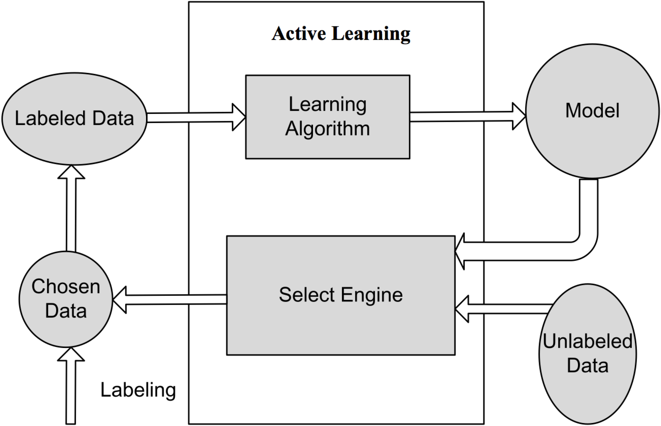

As shown in Fig. 1, active learning is mainly composed of learning algorithm and select machine, where learning algorithm is supervised learning method, such as support vector machines (SVM), and select machine is used to select data samples during each iteration according to uncertainty sampling [22]. During active learning process, learning algorithm first obtains an initial model from existing labeled data. Then, in each consecutive iteration, select machine picks up a few unlabeled data samples that are most uncertain according to current model. These data samples are used to update classification model after being labeled by human annotator. The iteration continues until stopping criterion is met.

However, the traditional active learning algorithms ignore the data distribution characteristics of training data, which in some cases may lead to local optimum [9]. As introduced before, active learning select labeled data according to current model, which means that active learning can not reach desirable results when current model is not well trained. In the first several iteration of active learning, the trained model usually does not perform well because the useful information is limited. Thus, the selected data samples is likely to contain redundant or even wrong information, which in turn influences the subsequent iteration even the final results.

Former research [3, 12, 13, 16] try to solve this problem by exploring distribution characteristics of unlabeled data. Although they improve the performance of active learning to some degree, effectiveness of these methods are constrained by some factors. More specifically, with the iteration goes on, the information containing in unlabeled data reduces, which means the explored information may not be enough for further utilizing. Another factor is the correctness of explored information. Due to lacking of labels, the information learned from unlabeled data maybe inaccurate. Applying these information will mislead the classification model and get even worse performance than traditional active learning.

In this paper, instead of exploring the distribution characteristics of original unlabeled data, we continuously utilize the information of labeled data mined by a manifold learning method. Manifold learning has been widely used to recover the intrinsic structure of high dimensional data and improve the resistance of machine learning methods [31, 32]. An advanced active learning algorithm based on low-rank transformation (LRT) for binary classification problems is proposed. During each iteration, after labeling the selected data samples, we first utilize the labeled data samples to obtain a subspace transformation. Then, the model is upgraded by the transformed data. The iteration goes on till the end of active learning.

The low-rank transformation is introduced to restore the low-dimensional subspaces of high-dimensional data and force a maximally separated structure for data from different subspaces. Therefore, the projected data are much easier to be classified. More importantly, active learning’s propriety of labeling data improves the performance of LRT. In particular, as more and more data samples are labeled, it is easier for LRT to achieve a better representation of whole dataset, which benefits the subsequent active learning process and promotes the accuracy of SVM classifier.

To evaluate the proposed algorithm, we compare it to other active learning methods with experiments on several standard datasets. The experimental results show that our method is superior to them in accuracy and convergence speed.

The rest of paper is structured as follows. Section 2 summaries related work. In Section 3, we introduce active learning SVM. Section 4 then presents the proposed algorithm and Section 5 evaluates our method on several benchmark datasets. We conclude in Section 6 with some discussion of the significance of our results and future work.

2. Related work

As is discussed in Section Introduction, prior endeavors in improving performance and efficiency of active learning mainly focus on exploring unlabeled data. Here, we summarize these works and discuss their limitations respectively.

[3, 16, 13] sought to improve the performance of active learning by different clustering algorithms. They applied selected clustering algorithm to original unlabeled dataset and divided data into different clusters. Based on the clustering results, the most uncertain data samples are selected as labeled data. Although these methods improved the classification accuracy of active learning, the performance of these methods highly depend on clustering algorithms. If the selected clustering algorithm cannot precisely explore the distribution of unlabeled data, performance of these methods will reduce to a large degree. [12] introduced a semi-supervised learning algorithm to active learning SVM. During each iteration, selected semi-supervised learning algorithm is used to extracted underlying manifolds of whole dataset and select most informative data samples for next iteration. However, most of semi-supervised learning algorithms also suffer the problem of being sensitive to initial state, combining active learning with these algorithms will weaken the robustness of active learning.

3. Active learning support vector machines

3.1 Support vector machines

Support Vector Machines [5] has been proven to be highly successful in binary classification problems both theoretically and empirically.

Given training data samples ${(x_{1},y_{1}),(x_{2},y_{2}),\ldots,(x_{N},y_{N})}$ , where $x_{i}\in\mathbb{R}^{n}$ and $y_{i}\in$ ${\pm}$ 1. SVM learns a classification hyper-plane based on the principle of maximum margin. The decision function SVM is as followed:

$\displaystyle f(x)=\textit{sign}(w^{T}\cdot x+b)$ (1)

where $w$ and $b$ determine the classification hyper-plane. When training data are linearly separable, this optimal hyper-plane is unique by maximizing the margin:

$\displaystyle\mathop{\text{max}}\limits_{w,b}\{\textit{min}\{\left\|x-x_{i}% \right\|:x\in\mathbb{R}^{n},w\cdot x+b=0\}\}$ (2)

However, when training data are not linearly separable, a punishment term $C>0$ is introduced to the original cost function. The following equations are the Wolfe dual problem [34] of the soft margin SVM.

$\displaystyle\mathop{\text{max}}\limits_{a}\sum_{i=1}^{N}\alpha_{i}-\frac{1}{2% }\sum_{i,j}\alpha_{i}\alpha_{j}y_{i}y_{j}\Phi(x_{i})\Phi(x_{j})$ (3) $\displaystyle\quad s.t.0\leqslant\alpha_{i}\leqslant C$ (4) $\displaystyle\quad\forall i,\sum_{i=1}^{N}\alpha_{i}y_{i}=0$ (5)

where $\Phi(\cdot)$ is a mapping from input space to feature space, $i$ is Lagrange multiplier.

In practice, most classification tasks are nonlinear. To solve these problems, we need to introduce kernel trick [2]. One of the widely used kernel is RBF kernel.

$\displaystyle K(x_{i},x_{j})=e^{-\gamma\left\|x_{i}-x_{j}\right\|^{2}}$ (6)

where $x_{i}$ and $x_{j}$ are two data samples and $\gamma$ is the parameter of kernel function.

Then $\Phi(\cdot)$ in Eq. (4) is replaced by Eq. (6), and the nonlinear classifier can be derived by solving the modified optimization problem. The optimal solution of $w$ and $b$ are:

$\displaystyle w=\sum_{i=1}^{N}\alpha_{i}^{*}y_{i}x_{i}$ (7)

$\displaystyle b=y_{i}-\sum_{i=1}^{N}\alpha_{i}^{*}y_{i}K(x_{i},x)$ (8)

3.2 Uncertainty sampling

As discussed in Introduction, the difference between active learning and standard supervised learning mainly lies in select machine. Select machine decides which data sample will be chosen in training process. Existing selecting criteria mainly are query by committee [28], expected model change [27], expected error reduction [25] and uncertainty sampling [17, 22]. Among these methods, the most widely used one is uncertainty sampling.

In this paper, uncertainty sampling is selected as select machine. In each iteration, the most uncertain data samples in unlabeled data pool are chosen for labeling. Uncertain data stand for the data samples whose label are hard to be determined according to current classification model. For example, in probability model (such as logistic regression), the data sample whose posterior probability nearly to be 0.5 should be chosen:

$\displaystyle x=\textit{argmin}|P_{f}(y|x)-0.5|$ (9)

As to discrimination model, the data sample with the largest uncertainty are those lies near the current hyper-plane. As to SVM, select engine choose data samples according to the following equation:

$\displaystyle x=\underset{x\in U}{\textit{argmin}}|\sum_{i=1}^{N}\alpha_{i}y_{% i}K(x_{i},x)+b|$ (10)

The algorithm procedure of active learning support vector machines with uncertainty sampling is shown in Table 1.

Table 1

Active learning support vector machines with uncertain sampling

Algorithm 1: Pool-based active learning support vector machines
Input: Unlabeled dataset $U^{(0)}$ , set of initial labeled samples $L^{(0)}$ , number of data samples selected in each iteration $k$ ;
Output: Classification model $f^{(t)}$ .
Step 1: Let $t=0$ , learn $f^{(0)}$ from $L^{(0)}$ by SVM;
Step 2: $t=t+1$ ;
Step 3: Select $k$ most uncertain data samples from $U^{(t)}$ according to Eq. (10) and label them;
Step 4: Update $L^{(t)}$ and $U^{(t)}$ ;
Step 5: Learn $f^{(t)}$ from $L^{(t)}$ ;
Step 6: Repeat steps 2–5, until stopping criterion is met;
Step 7: Return $f^{(t)}$ .

4. Active learning with low-rank transformation

As presented in Introduction, improving the performance of active learning by taking advantage of data distribution characteristic has achieved success due to the explosion of data mining methods. However, current strategies mainly focus on exploring the distribution characteristic of unlabeled data and suffer certain problems. In this paper, instead of exploring the data distribution characteristic of unlabeled data, we focus on extracting the information containing in labeled data samples.

4.1 Low-rank transformation

Labeled data samples are only used to derive classification model in traditional active learning. However, in this paper, we learn a low-rank transformation $\Psi$ from labeled set. By conducting this transformation $\Psi$ , data samples can be projected to several low-dimensional subspaces, where the distance of data samples between different categories become larger. Details of low-rank transformation is presented as follows.

Suppose the dimensionality of input space $X$ is $d$ , then transformation can be described as a matrix $P(d\times d)$ . As to labeled data $L={(x_{i},y_{i})}$ , the projected data can be written as follows:

$\displaystyle L_{\Psi}={(Px_{i},y_{i})}$ (11)

Let $\{S_{c}\}_{c=1}^{c}$ be $C$ subspaces of input data data $X=\{x_{i}\}_{i=1}^{N}$ , where $x_{i}\in\mathbb{R}^{n}$ and $X_{c}=\{x|x\in X,x\in S_{c}\}$ . thus $X$ is equal to $[X_{1},X_{2},\ldots,X_{C}]$ . In order to explore the subspaces structure from original data, proper transformation is required.

Suppose the projected data can be written as:

$\displaystyle PX=[PX_{1},PX_{2},\ldots,PX_{c}]$ (12)

In order to find these subspaces, $P X$ should conform to the following two attributes:

•

Data samples in same subspace should be as close as possible, which means $\textit{rank}(PX_{1})$ , $\textit{rank}(PX_{2})$ , $\ldots$ $\textit{rank}(PX_{C})$ should be as small as possible;

•

rank(PX) should be as large as possible, given that the distance between different subspaces should be so far as possible.

According to the aforementioned attributes, the optimization function of finding $P$ can be written as follows:

$\displaystyle\mathop{\text{max}}\limits_{p}\sum_{c=1}^{C}\textit{rank}(PX_{c})% -\textit{rank(PX)}$ (13)

$\displaystyle s.t.\|P\|_{2}=1$ (14)

where the constraint is to prevent the condition of $P=$ 0.

Given matrices $A$ and $B$ of same dimensionality, and $[A,B]$ be the concatenation of $A$ and $B$ . We have the following inequation according to [10]:

$\displaystyle\textit{rank(A, B)}\leqslant\textit{rank(A)}+\textit{rank(B)}$ (15)

with equality if and only if $A$ and $B$ are disjoint. According to Eq. (15), we can easily get that:

$\displaystyle\textit{rank(PX)}\leqslant\textit{rank}(PX_{1})+\textit{rank}(PX_% {1},PX_{2},\ldots,PX_{C})\leqslant\sum_{c=1}^{C}\textit{rank}(PX_{c})$ (16)

with equality if matrices are independent. When the matrices $PX_{c}$ are independent, the Eq. (14) reaches the minimum 0. However, being independent does not mean the distances between each matrix are maximized. For example, two lines only intersect at origin, which means they are independent. However, they have the maximum distance only when angle between them are $\pi/2$ . Thus, function Eq. (14) has optimal solution other than 0.

Table 2

Algorithm of computing sub-gradient of matrix nuclear norm

Algorithm 2: Sub-gradient of matrix nuclear norm
Input: matrix $A$ , threshold value $\delta$ ;
Output: $\partial\\|A\\|_{*}$ .
Step 1: Calculate Singular Value Decomposition (SVD) of $A$ , $A=U\Sigma V^{T}$ and $\Sigma=diag(\sigma_{1},\sigma_{2},\ldots,\sigma_{p})$ , where $\sigma_{1}>\sigma_{2}>\ldots>\sigma_{p}$ are singular value of $A$ ;
Step 2: Let the number of singular values which are less than $\delta$ is $s$ , and $k=min(m,n)$ ;
Step 3: Let $U=[U1,U2]$ and $V=[V1,V2]$ ,where the number of columns of $U_{1}$ , $V_{1}$ is $s$ ;
Step 4: If $s>$ 0, randomly create a matrix $B$ $(m-k+s)\times(m-k+s)$ , then let $B=\frac{B}{\\|B\\|}$ if $s=0$ , then $B=$ 0;
Step 5: Compute sub-gradient $\partial\\|A\\|_{*}=U_{1}V_{1}^{T}+U_{2}BV_{2}^{T}$ ;
Step 6: Return $\partial\\|A\\|_{*}$

We use the nuclear norm of matrix to replace rank in Eq. (14), because nuclear norm is the best convex approximation of the rank function in the rank optimization [6, 24]. Then, the optimizatioin function can be described as follows:

$\displaystyle\mathop{\text{max}}\limits_{T}\sum_{c=1}^{C}\|PX_{c}\|_{*}-\|PX\|% _{*}$ (17)

$\displaystyle s.t.\|P\|_{2}=1$ (18)

As to matrix $A$ , the nuclear norm of $A$ equals to the sum of all the singular values of $A$ .

Since this optimization problem is the subtraction of two convex term, it should be solved by concave-convex procedure [23].

The basic idea of concave-convex procedure is to obtain the optimal solution of non-convex problem by iteratively solving the sub-problem of original problem. Sub-problem is constructed by replacing the concave terms in original optimization function with their one-order Taylor series [30, 36]. $J(P)$ can be written as the sum of a convex term and a concave term.

$\displaystyle J(P)=J_{vex}(P)+J_{cav}(P)$ (19)

$\displaystyle J_{vex}(P)=\sum_{c=1}^{C}\|PX_{c}\|_{*}$ (20)

$\displaystyle J_{cav}(P)=-\|PX\|_{*}$ (21)

Then sub-problem of Eq. (17) is:

$\displaystyle J_{sub}(P)=P^{(t+1)}=\mathop{\text{max}}\limits_{p}\sum_{c=1}^{C% }\|PX_{c}\|_{*}-\partial\|P^{(t)}X\|X^{T}P^{T}$ (22)

$P(0)=I$ is the initial state. Because nuclear norm is non-differential, in order to solve Eq. (22), we introduce sub-gradient of matrix nuclear norm. According to [33], the detailed algorithm is shown as follows.

Based on Algorithm 2, the sub-gradient of $J_{sub}(P)$ is as follows:

$\displaystyle\sum_{c=1}^{C}\partial\|PX_{c}\|_{*}X_{c}^{T}-\partial\|P^{(t)}X% \|_{*}X^{T}$ (23)

Given the sub-gradient of $J_{sub}(P)$ , and step length $\eta$ , the sub-problem Eq. (22) can be solved by the algorithms presented in Table 3.

Table 3

Algorithm of solving concave-convex sub-problem

Algorithm 3: Sub-gradient method for concave-convex sub-problem.

Input:

P^{(t)}

, step length

\eta

convergence precision

\varepsilon

;

Output:

P^{(t+1)}

Step 1: Calculate

P_{0}=P^{(t)}

;

Step 2: Compute sub-gradient according to Eq. (23);

Step 3: Let

P_{1}=P_{0}-\eta\partial J_{sub}

;

Step 4: If

|J_{sub}(P_{1})-J_{sub}(P_{0})|>\varepsilon_{1}

, then let

P_{0}=P_{1}

, and return to step 2;

Step 5: Let

P_{1}=\frac{P_{1}}{\|P_{1}\|}

;

Step 6: Let

P^{(t+1)}=P_{1}

and return

p^{(t+1)}

According to the former analysis, we derive the algorithm of computing transformation matrix $P$ by concave-convex procedure, whihc is shown in Table 4. Note that the hyper-parameter $a$ in Algorithm 4 is usually set as 1–3.

Table 4

Algorithm of computing transformation matrix $P$

Algorithm 4: Computing $P$ by Concave-Convex Procedure.
Input: $X=[X_{1},X_{2},\ldots,X_{C}]$ , number of iteration $a$ ;
Output: $P$ .
Step 1: $t=0$ , $P^{(t)}=I$ ;
Step 2: Compute $P^{(t+1)}$ according to algorithm 3;
Step 3: If $t<a$ , let $t=t+1$ , return to step 2;
Step 4: Let $P=P^{(a)}$ , and return $P$ .

4.2 Proposed Method

After introducing LRT, we present the proposed algorithm. This algorithm embeds LRT into each iteration of active learning SVM. More specifically, during each iteration, besides updating the classification model, the labeled data samples are used to calculate the transformation matrix $P$ . Then, all of the training data are projected to several subspaces by low-rank transformation. Because LRT is a linear transformation method, we conduct the transformation in the same kernel space as SVM in case that the dataset contains non-linear attributes. The details of the algorithm are shown in the Table 5.

Table 5
Active learning with low-rank transformation

Algorithm 5: Active learning with low-rank transformation
Input: Unlabeled dataset X, set of initial labeled samples’ index $I_{L}^{(0)}$ ,
number of data samples selected each iteration $k$ ;
Output: Classification model $f^{(t)}$ , and transformation matrix $P^{(t)}$ .
Step 1: Let $t=0$ , $P^{(0)}=I$ , and create $I_{U}^{(0)}$ to store of indexes unlabeled data samples;
Step 2: Create labeled data samples set $L^{(t)}$ , and learn $f^{(t)}$ from $L^{(t)}$ by SVM;
Step 3: Select $k$ most uncertain data samples from $U^{(t)}$ , according to Eq. (10);
Step 4: Label the selected data and update $I_{U}^{(t)}$ and $I_{L}^{(t)}$ ;
Step 5: Update labeled samples set $L^{(t)}$ and learn transformation matrix $P^{(t)}$ according to Algorithm 4;
Step 6: Projected whole dataset to feature space by transformation matrix $P^{(t)}$ : $X^{(t+1)}=P^{(t)}X^{(t)}$ ;
Step 7: $t=t+1$ ;
Step 8: Repeat step 2-7, until stopping criterion is met;
Step 9: Return $f^{(t)}$ and $P^{(t)}$ .

As shown in Table 5, labeled samples set $L$ is used to learn a transformation matrix $P$ and SVM classifier is updated in feature space during each iteration. As iteration goes on, the scale of $L$ grows too. The learned transformation matrix $P$ will explore more information about whole dataset. Thus, it will be easier for $P$ to show the intrinsic subspaces of dataset $X$ , which means the distance between subspaces of the projected data $P X$ keeps becoming larger. Updating classification model from the projected data will improve the performance of SVM classifier.

In practice, threshold value $\delta$ , step length $\eta$ and convergence precision $\varepsilon$ are parameters needed to be set. These parameters mainly influence the computation process instead of the transformation matrix. That is to say, unlike hyper-parameter such as $C$ of SVM, these parameters have no influence on $P$ and the final classification result. In this paper, we set that $\delta=$ 0.01, $\eta=$ 0.02 and $\varepsilon=$ 0.1.

4.3 Time complexity of proposed method

The Time complexity of the proposed method depends on the computational cost of SVM in Algorithm 1 and LRT in Algorithm 4.

As to SVM, we introduce a relatively fast algorithm called LASVM [4]. It requires the number of operations proportional to the number of support vector $s$ . Suppose performing $K$ epoches of iterations, then time complexity is proportional to $n s K$ , where $n$ is the number of data samples in dataset. So the asymptotic time is between O( $n^{2}$ ) and O( $n^{3}$ ).

When it comes to LRT, the time complexity of Algorithm 2 is the same of asymptotic time of SVD, which is O( $mn^{2}$ ) ( $n\leqslant m$ ) for a matrix $A$ $(m\times n)$ . Then the time complexity of $\partial J_{sub}$ in algorithm 3 is O( $n^{3}$ ). Because both algorithm 3 and algorithm 4 require finite time of calculating $\partial J_{sub}$ , the asymptotic time complexity of LRT is O( $n^{3}$ ).

Since the proposed algorithm requires finite times of iteration, and computes one time of $P$ and $f$ during each iteration, the time complexity of proposed method is O( $n^{3}$ ), where $n$ is the number of data samples.

5. Evaluations

To evaluate the performance of the proposed method, we conduct experiments on several widely used benchmark datasets. All of these datasets come from LIBSVW [7].In order to show the effectiveness of this method, other popular algorithms are used for comparison. The main idea of these algorithms are introduced as follows:

•
Active learning SVM: standard active learning algorithms, the details of this algorithm is shown in Table 1;
•
Passive learning: randomly selects certain number of data samples in each iteration, this method can be considered as traditional support vector machines;
•
Active learning with principle component analysis (PCA): since the proposed method is based on the manifold assumption [37], we compare it with another manifold learning method. This method applies PCA to extract main features of unlabeled data before active learning process [8, 11, 26].

Table 6
Statistic indexes of error rates on DNA 1 vs others over 100 runs

ALSVM Proposed Passive ALPCA

MEAN 0.1545 0.0426 0.1867 0.1058

STDEV 0.0632 0.0061 0.0049 0.0465

MAX 0.3260 0.0605 0.1975 0.1680

MIN 0.0585 0.0209 0.1775 0.0405

Table 7
Statistic indexes of error rates on DNA 2 vs others over 100 runs

ALSVM Proposed Passive ALPCA

MEAN 0.1462 0.0318 0.1473 0.1237

STDEV 0.0911 0.0052 0.0789 0.0472

MAX 0.4500 0.4650 0.3915 0.1835

MIN 0.0495 0.0245 0.0780 0.0575

Figure 2.
Average error rates on DNA 1 vs others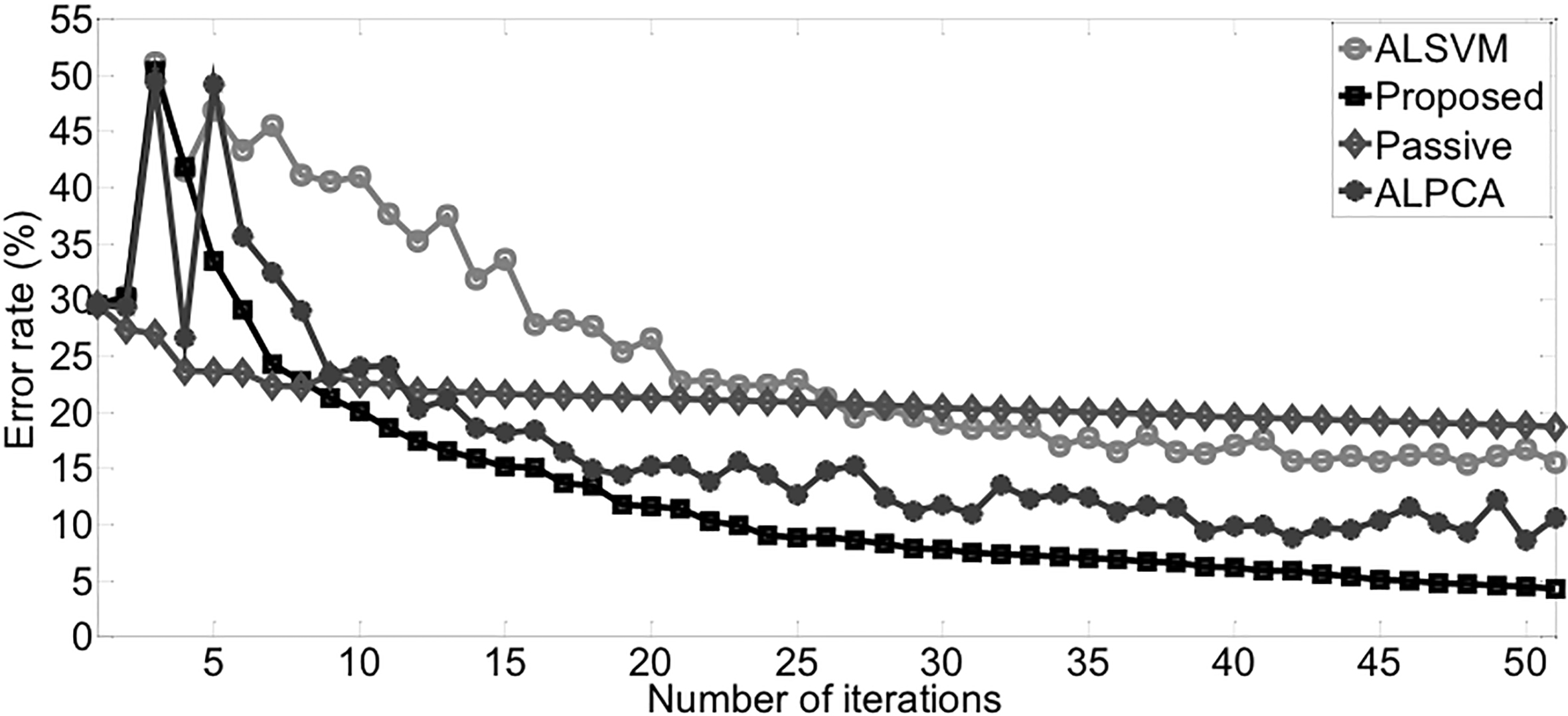

5.1 Experiments on DNA

	ALSVM	Proposed	Passive	ALPCA
MEAN	0.1545	0.0426	0.1867	0.1058
STDEV	0.0632	0.0061	0.0049	0.0465
MAX	0.3260	0.0605	0.1975	0.1680
MIN	0.0585	0.0209	0.1775	0.0405

	ALSVM	Proposed	Passive	ALPCA
MEAN	0.1462	0.0318	0.1473	0.1237
STDEV	0.0911	0.0052	0.0789	0.0472
MAX	0.4500	0.4650	0.3915	0.1835
MIN	0.0495	0.0245	0.0780	0.0575

Firstly, we evaluate our method on DNA dataset [7]. DNA dataset contains 2000 data samples of 3 different classes. We conduct three experiments on this dataset, each experiment distinguishes one class of data samples. We reset the labels of data samples and convert the problem to binary classification. This strategy has been widely used when SVM is applied to multi-classes classification problems [19].

Table 8
Statistic indexes of error rates on DNA 3 vs others over 100 runs

	ALSVM	Proposed	Passive	ALPCA
MEAN	0.0871	0.0862	0.1663	0.0865
STDEV	0.0428	0.0096	0.0658	0.0097
MAX	0.4525	0.1235	0.3485	0.0910
MIN	0.0605	0.0665	0.0815	0.0580

Figure 3.

Average error rates on DNA 2 vs others.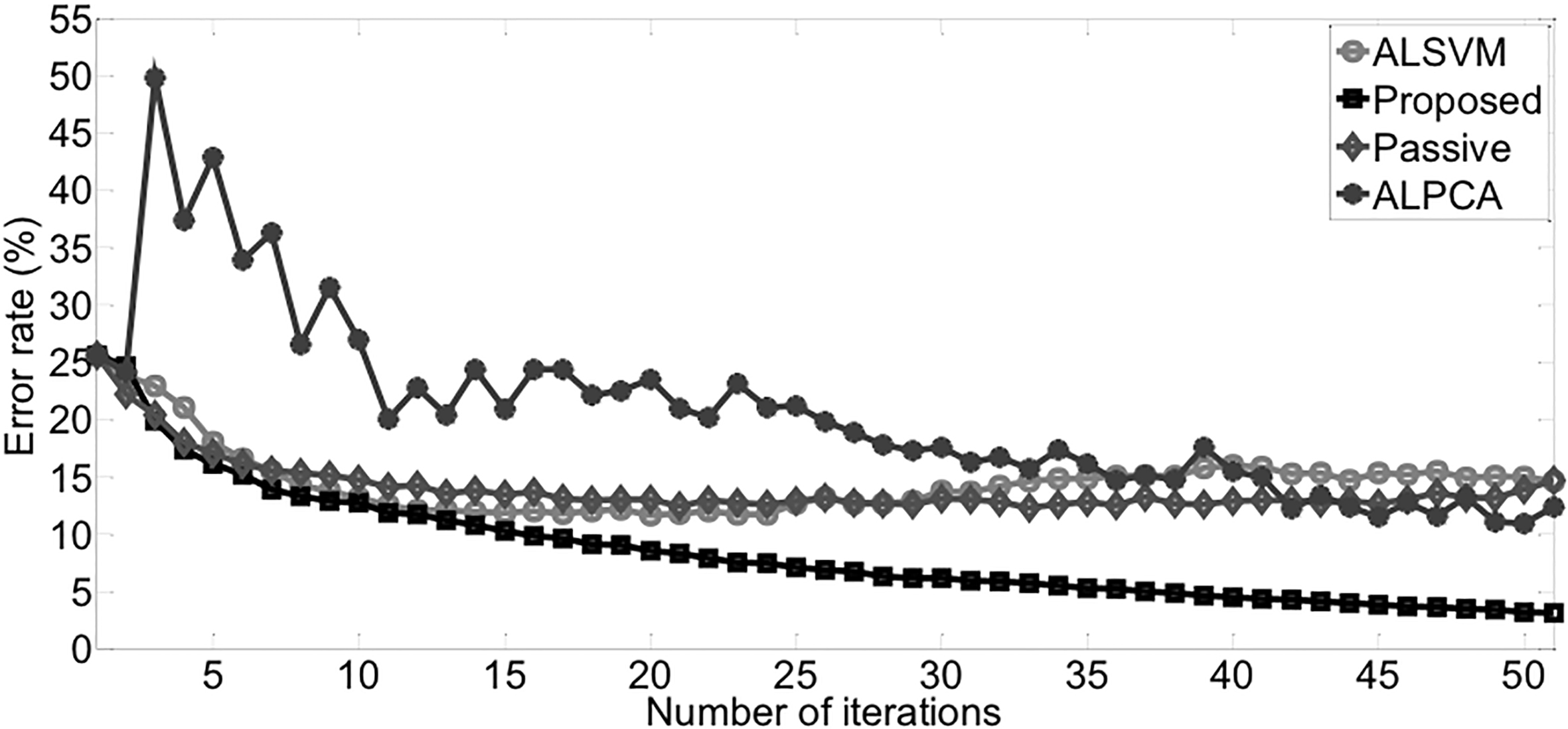

Figure 4.

Average error rates on DNA 3 vs others.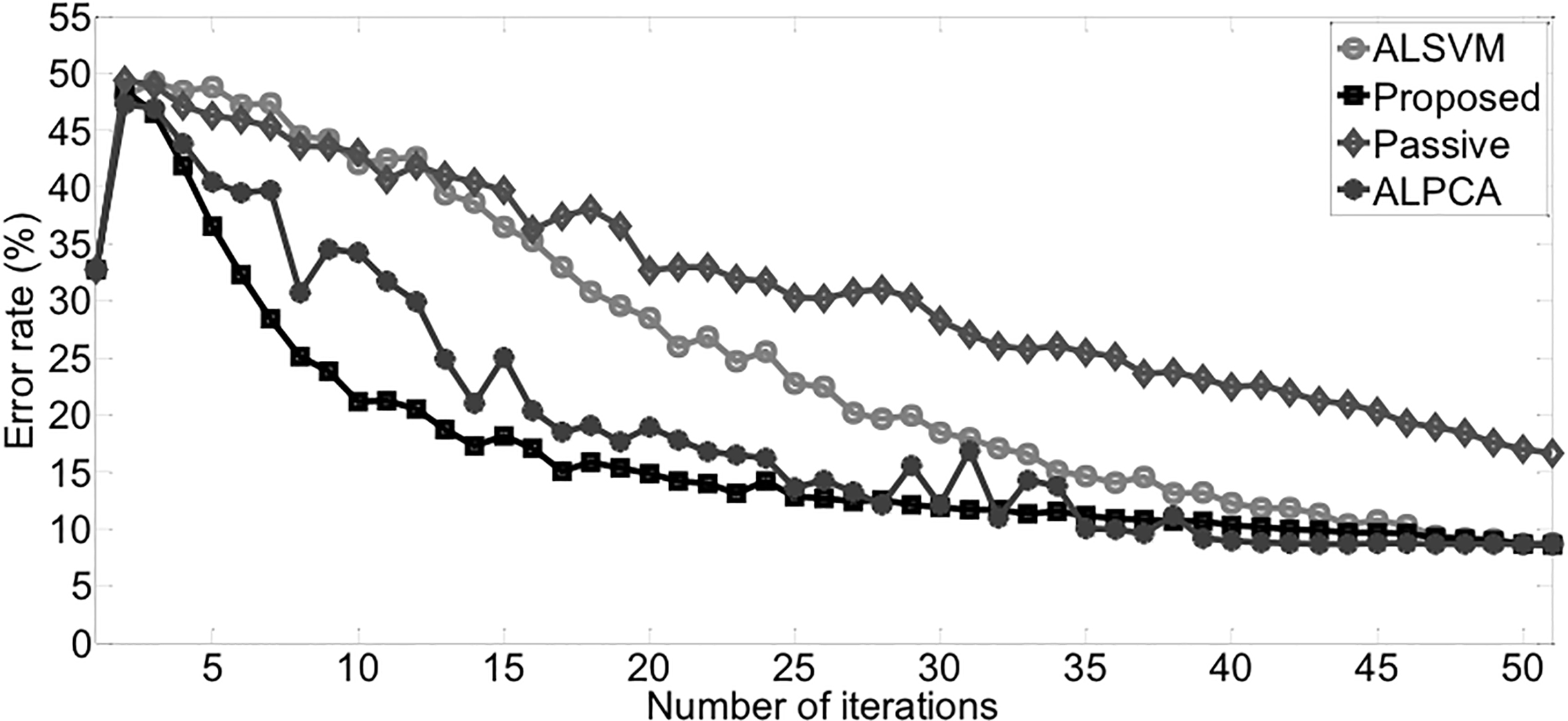

Original dataset is divided into training set and test set. The labels of original training set are hid and only the selected samples will be labeled during training process. Hyper-parameter $C$ , $\gamma$ of SVM are chosen by Grid search and cross validation [15]. In this experiment, parameters are set as $C=$ 100, $\gamma=$ 1.

In each run, we choose 10 data samples as initial labeled set, and during each iteration, 5 data samples are selected from unlabeled data pool. We run these algorithm 100 times, and draw the average error rates according to number of iterations.

5.1.1 DNA 1 vs others

Figure 2 shows the results of recognizing class $1$ , which means that we label the data samples belonging to first class with $+1$ , and set the rest data samples with label $-1$ . From the figure, we can see that proposed algorithm beats the other methods in error rate after ninth iteration. The figure also shows that our method has the fastest convergence speed and lowest error rate after fiftieth iteration.

Four statistics indexes of error rates after fiftieth iteration are shown in Table 6, these results are calculated from the final error rates over 100 runs. Bold face means the best performance. STDEV means the standard deviation of the final error rates.

Table 9
Statistic indexes of error rates on w5a over 100 runs

	ALSVM	Proposed	Passive	ALPCA
MEAN	0.1575	0.0474	0.0913	0.2426
STDEV	0.1632	0.0425	0.1545	0.1230
MAX	0.7685	0.1413	0.9127	0.5319
MIN	0.0187	0.0195	0.0254	0.0311

Table 10

Statistic indexes of error rates on letter D vs O over 100 runs

	ALSVM	Proposed	Passive	ALPCA
MEAN	0.0205	0.0137	0.0716	0.0446
STDEV	0.0105	0.0079	0.0269	0.0181
MAX	0.0520	0.0410	0.1860	0.0734
MIN	0.0060	0.0043	0.0282	0.0188

Table 11

Statistic indexes of error rates on letter M vs N over 100 runs

	ALSVM	Proposed	Passive	ALPCA
MEAN	0.0219	0.0172	0.0611	0.0111
STDEV	0.0285	0.0079	0.0177	0.0028
MAX	0.1576	0.0586	0.1155	0.0165
MIN	0.0041	0.0058	0.0330	0.0074

Figure 5.

Average error rates on w5a.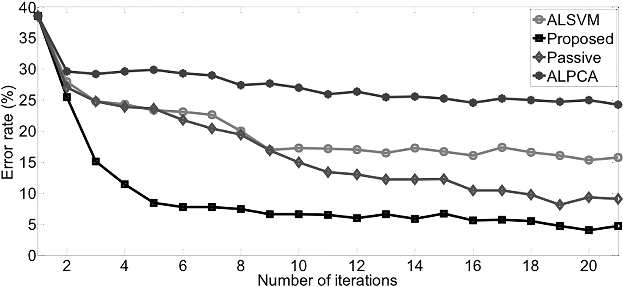

Table 6 shows that the proposed method is superior to other methods in three indexes, which indicates that besides achieving best classification performance, proposed method is more robust to initial state than other methods.

5.1.2 DNA 2 vs others

The average error rates of classifying class 2 are shown in Fig. 3. The proposed method obtains the fastest convergence speed and the lowest average error rate. Table 7 shows that proposed method stands out from other algorithms in all of four indexes.

5.1.3 DNA 3 vs others

Figure 6.

Average error rates on letter D vs O.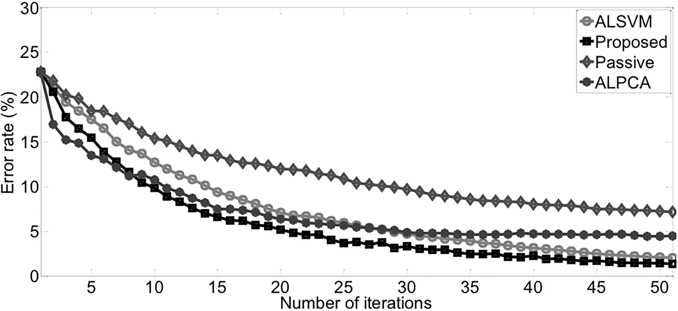

Figure 7.

Average error rates on letter M vs N.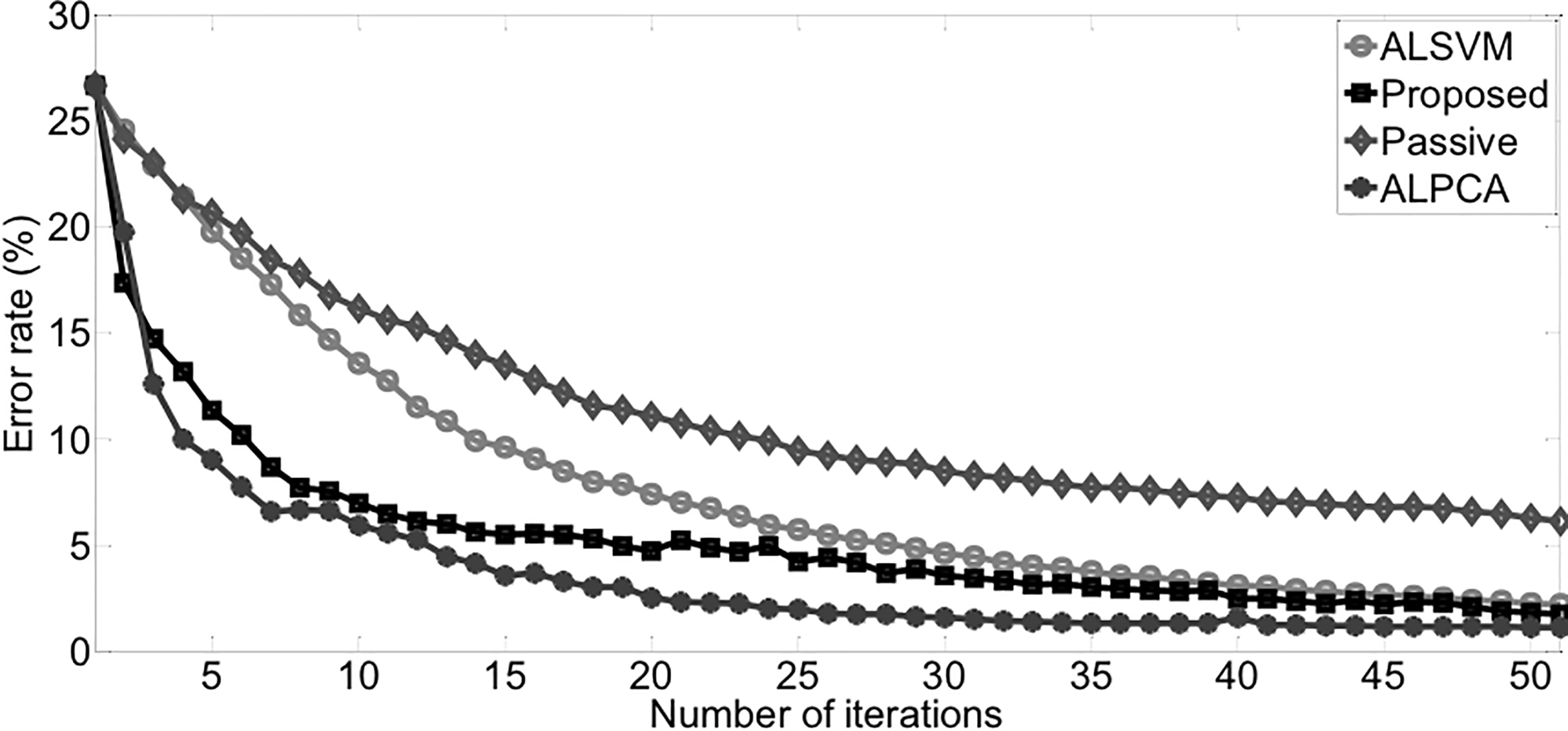

Figure 4 shows the results of DNA 3 vs others. In this experiment, the average error rate of proposed is slightly lower than ALPCA and ALSVM. This experiment demonstrates the advantage of active learning over passive learning methods. Based on the MEAS and STDEV in Table 8, proposed method achieves the best robustness over other methods.

Table 12

Results of experiments on other datasets over 20 runs

Dataset	C	r	k	Iterations	ALSVM	Proposed	Passive	ALPCA
Ala	100	0.1	5	50	0.1514	0.1439	0.1822	0.1608
					0.0094	0.0087	0.0118	0.0259
Australia	100	0.001	5	20	0.1629	0.1428	0.1757	0.1857
					0.0619	0.0098	0.0542	0.0817
Breast-cancer	10	1	3	50	0.0233	0.0204	0.0360	0.0361
					0.0072	0.0069	0.0081	0.0079
Diabets	10	0.1	3	40	0.2564	0.2365	0.2665	0.3671
					0.0272	0.0345	0.0406	0.0439
Fourclass	1000	1	3	15	0.2357	0.2046	0.2391	0.2357
					0.0678	0.0623	0.0820	0.0678
German	1000	0.001	3	40	0.2855	0.3041	0.3541	0.4530
					0.0445	0.0978	0.0771	0.1025
Heart	100	0.001	3	45	0.2430	0.1735	0.2944	0.2833
					0.1269	0.0870	0.1276	0.1255
Ionosphere	1	0.1	4	50	0.1185	0.1818	0.1092	0.1439
					0.0826	0.0693	0.0305	0.0480
Liver-disorders	100	0.1	3	45	0.4291	0.3191	0.4257	0.4439
					0.0779	0.0482	0.0724	0.0563
Letter	100	1	5	50	0.0037	0.0206	0.0112	0.0288
B vs P					0.0091	0.0312	0.0044	0.0038
Satimage	4	4	5	50	0.0246	0.0069	0.0549	0.0409
1 vs others					0.0374	0.0028	0.0159	0.0209
Satimage	4	4	5	50	0.0451	0.0654	0.0819	0.1360
6 vs others					0.0142	0.0113	0.0495	0.0897
Svmguide1	2	2	5	50	0.5501	0.3617	0.3297	0.0640
					0.1458	0.1839	0.0623	0.0085
Svmguide3	128	0.125	5	50	0.4428	0.1853	0.3119	0.2963
					0.2068	0.0167	0.1964	0.1592
Splice	10	0.01	5	44	0.1826	0.1592	0.2462	0.1608
					0.0489	0.0179	0.0548	0.0225
Usps	10	0.01	10	15	0.0021	0.0018	0.0084	0.0021
1 vs 7					0.0009	0.0005	0.0021	0.0006
Usps	10	0.01	10	15	0.0022	0.0013	0.0115	0.0023
3 vs 8					0.0011	0.0005	0.0035	0.0003
W2a	100	0.01	5	20	0.3310	0.0566	0.1967	0.4842
					0.2409	0.0574	0.2422	0.1567

5.2 Experiment on w5a

W5a is a text classification dataset, where label means whether a web page belongs to a certain category or not. The dataset contains 9888 samples, and each sample has 300 features of 0 or 1 [21]. We choose 5 data samples of each class for initialization and during each iteration, 5 most uncertain instances are labeled. The parameters are set as: $C=$ 100, $\gamma=$ 1.We also run the experiments 100 times.

The results of this experiment are shown in Fig. 5 and Table 9. Proposed method also beats other algorithms from second iteration and it achieves the lowest standard deviation. Once again, the proposed algorithm is more robust than other methods with respect to initial labled data.

5.3 Experiments on letter

This experiment is conducted on letter dataset. It is a handwritten characters recognition dataset with 20000 data samples of 26 different characters [7]. In this experiment, we choose two subsets of letter: ‘D’ vs ‘O’ and ‘M’ vs ‘N’.

We also run the experiments 100 times, each time with 50 iterations. The hyper-parameters are $C=$ 100, $\gamma=$ 1. Initially, we choose 5 data samples of each category, and during each iteration we label 5 data samples.

5.3.1 Letter D vs O

The results of letter D vs O are shown in Fig. 6 and Table 10. The proposed method slightly surpass other methods in classification performance and robustness. Similar to the experiment on DNA 3 vs other, active learning methods achieve lower error rate and better robustness than passive learning.

5.3.2 Letter M vs N

Figure 7 and Table 11 present the results of experiment on letter M vs N. ALPCA achieve the best classification performance and robustness on this dataset. Proposed method is not far behind. This experiment indicates that taking advantage of the data distribution information can improve the performance of active learning.

5.4 Other datasets

Final error rates and statistics indexes of different methods on some other datasets [1, 7] are shown in Table 12. These experiments are all binary classification and the hyper-parameters are also listed.

In Table 12, each cell has two numbers, where the upper one is the average of final error rates and the other is the standard deviation of the final error rates. From the table, we can find out the proposed method achieves lowest error rate on 13 out of 18 datasets, and lowest standard deviation on 12 out of 18 datasets. The results indicate that proposed algorithm obtains better generalization ability and are more robust than other methods. From the table, we can also draw the conclusion that active learning beats passive learning in most of scenarios.

6. Conclusion

We propose a novel active learning algorithm to improving the performance and robustness of active learning. The algorithm is designed based on an analysis of the limitations of current methods. In particular, LRT can project data to a feature space where data samples belonging to different classes are easier to be separate. Training the classifier on projected data will improve the performance of final SVM model.

Empirically, we have demonstrated that three widely used algorithms are insufficient when compared with proposed method. Applying our new algorithm to more than 20 standard datasets, we have shown that our algorithm effectively improves the classification accuracy. In addition, statistic indexes show our algorithm also improves the robustness of final classifier to initial state.

Future work will entail investigating other data transformation methods, e.g. adaptive manifold learning [37], to lower the computational complexity of our algorithm, and further explore how to utilize the information of labeled data and unlabeled data at the same time.

References

Asuncion

and Newman

, Uci machine learning repository, 2007.

Baudat

and Anouar

, Kernel-based methods and function approximation, In Neural Networks, 2001. Proceedings. IJCNN’01. International Joint Conference on, volume 2, IEEE, 2001, pages 1244–1249.

Bodó

Minier

and Csató

, Active learning with clustering, In Active Learning and Experimental Design@ AISTATS, 2011, pages 127–139.

Bordes

Ertekin

Weston

and Bottou

, Fast kernel classifiers with online and active learning, Journal of Machine Learning Research 6(Sep) (2005), 1579–1619.

Burges

C.J.

, A tutorial on support vector machines for pattern recognition, Data Mining and Knowledge Discovery 2(2) (1998), 121–167.

Candès

E.J.

and Wright

, Robust principal component analysis? Journal of the ACM (JACM) 58(3) (2011), 11.

Chang

C.-C.

and Lin

C.-J.

, Libsvm: a library for support vector machines, ACM Transactions on Intelligent Systems and Technology (TIST) 2(3) (2011), 27.

Curtin

R.R.

Cline

J.R.

Slagle

N.P.

March

W.B.

Ram

Mehta

N.A.

and Gray

A.G.

, Mlpack: A scalable c++ machine learning library, Journal of Machine Learning Research 14(Mar) (2013), 801–805.

Dasgupta

and Hsu

, Hierarchical sampling for active learning, In Proceedings of the 25th International Conference on Machine Learning, ACM, 2008, pages 208–215.

10.

Elhamifar

and Vidal

, Sparse subspace clustering: Algorithm, theory and applications, IEEE Transactions on Pattern Analysis and Machine Intelligence 35(11) (2013), 2765–2781.

11.

Gong

and Yang

, An improved active learning method based on feature selection, 2015.

12.

C.-J.

and Yang

Y.-P.

, A batch-mode active learning svm method based on semi-supervised clustering, Intelligent Data Analysis 19(2) (2015), 345–358.

13.

Guo

Zhong

and Yang

, Spectral clustering based active learning with applications to text classification, In MATEC Web of Conferences, volume 56. EDP Sciences, 2016.

14.

Hoi

S.C.

Jin

Zhu

and Lyu

M.R.

, Semisupervised svm batch mode active learning with applications to image retrieval, ACM Transactions on Information Systems (TOIS) 27(3) (2009), 16.

15.

Hsu

C.-W.

and Lin

C.-J.

, A comparison of methods for multiclass support vector machines, IEEE transactions on Neural Networks 13(2) (2002), 415–425.

16.

Xie

and Maybank

, Unsupervised active learning based on hierarchical graph-theoretic clustering, IEEE Transactions on Systems, Man and Cybernetics, Part B (Cybernetics) 39(5) (2009), 1147–1161.

17.

Janssen

, Monte-carlo based uncertainty analysis: Sampling efficiency and sampling convergence, Reliability Engineering & System Safety 109 (2013), 123–132.

18.

Joshi

A.J.

Porikli

and Papanikolopoulos

, Multi-class active learning for image classification, In Computer Vision and Pattern Recognition, 2009. CVPR 2009. IEEE Conference on, IEEE, 2009, pages 2372–2379.

19.

Lee

C.-P.

and Lin

C.-J.

, A study on l2-loss (squared hinge-loss) multiclass svm, Neural Computation 25(5) (2013), 1302–1323.

20.

Nissim

Moskovitch

Rokach

and Elovici

, Novel active learning methods for enhanced pc malware detection in windows os, Expert Systems with Applications 41(13) (2014), 5843–5857.

21.

Platt

et al., Sequential minimal optimization: A fast algorithm for training support vector machines, 1998.

22.

Prudencio

R.B.

Soares

and Ludermir

T.B.

, Uncertainty sampling methods for selecting datasets in active meta-learning, In Neural Networks (IJCNN), The 2011 International Joint Conference on, IEEE, 2011, pages 1082–1089.

23.

Qiu

and Sapiro

, Learning transformations for clustering and classification, Journal of Machine Learning Research 16 (2015), 187–225.

24.

Recht

Fazel

and Parrilo

P.A.

, Guaranteed minimum-rank solutions of linear matrix equations via nuclear norm minimization, SIAM Review 52(3) (2010), 471–501.

25.

Roy

and McCallum

, Toward optimal active learning through monte carlo estimation of error reduction, ICML, Williamstown, 2001, pp. 441–448.

26.

Sanderson

, Armadillo: An open source c++ linear algebra library for fast prototyping and computationally intensive experiments, 2010.

27.

Settles

Craven

and Ray

, Multiple-instance active learning, In Advances in Neural Information Processing Systems, 2008, pp. 1289–1296.

28.

Shao

Tong

and Suzuki

, Query by committee in a heterogeneous environment, In International Conference on Advanced Data Mining and Applications, Springer, 2012, pp. 186–198.

29.

Sivaraman

and Trivedi

M.M.

, A general active-learning framework for on-road vehicle recognition and tracking, IEEE Transactions on Intelligent Transportation Systems 11(2) (2010), 267–276.

30.

Sriperumbudur

B.K.

and Lanckriet

G.R.

, A proof of convergence of the concave-convex procedure using zangwill’s theory, Neural Computation 24(6) (2012), 1391–1407.

31.

Wang

Guo

Zhang

Ororbia

Alexander

Xing

Giles

C.L.

and Liu

, Learning adversary-resistant deep neural networks, arXiv preprint arXiv:1612.01401, 2016.

32.

Wang

Guo

Zhang

Xing

Giles

C.L.

and Liu

, Random feature nullification for adversary resistant deep architecture, arXiv preprint arXiv:1610.01239, 2016.

33.

Watson

G.A.

, Characterization of the subdifferential of some matrix norms, Linear Algebra and Its Applications 170 (1992), 33–45.

34.

Wolfe

, A duality theorem for non-linear programming, Quarterly of applied mathematics, 1961, pp. 239–244.

35.

Yang

et al., Automatically labeling video data using multi-class active learning, In Computer Vision, 2003. Proceedings. Ninth IEEE International Conference on, IEEE, 2003, pp. 516–523.

36.

Yuille

A.L.

and Rangarajan

, The concave-convex procedure, Neural Computation 15(4) (2003), 915–936.

37.

Zhang

Wang

and Zha

, Adaptive manifold learning, IEEE Transactions on Pattern Analysis and Machine Intelligence 34(2) (2012), 253–265.

Active learning support vector machines with low-rank transformation

Abstract

Keywords

1. Introduction

3. Active learning support vector machines

3.1 Support vector machines

4.1 Low-rank transformation

Table 5 Active learning with low-rank transformation

5. Evaluations

Table 8 Statistic indexes of error rates on DNA 3 vs others over 100 runs

Table 9 Statistic indexes of error rates on w5a over 100 runs

5.1.3 DNA 3 vs others

5.3 Experiments on letter

5.3.1 Letter D vs O

5.3.2 Letter M vs N

5.4 Other datasets

6. Conclusion

References

Table 5
Active learning with low-rank transformation

Table 8
Statistic indexes of error rates on DNA 3 vs others over 100 runs

Table 9
Statistic indexes of error rates on w5a over 100 runs