Asymptotics of sign-changing patterns in hysteretic systems with diffusive thresholds

Abstract

We consider a reaction–diffusion system including discontinuous hysteretic relay operators in reaction terms. This system is motivated by an epigenetic model that describes the evolution of a population of organisms which can switch their phenotype in response to changes of the state of the environment. The model exhibits formation of patterns in the space of distributions of the phenotypes over the range of admissible switching strategies. We propose asymptotic formulas for the pattern and the process of its formation.

Keywords

reaction–diffusion equations patterns phenotype switching hysteresis free boundary asymptotic limit of slow diffusion

1. Introduction

In this paper, we consider a reaction–diffusion equation that includes discontinuous two-state two-threshold relay operators. This equation was proposed as a model for dynamics of a population of bacteria that can switch their phenotype in response to changes of the environment [17,20]. The model exhibits formation of patterns in the space of distributions of the two phenotypes over an admissible range of the switching thresholds. The convergence of solutions to a stationary pattern observed numerically in [17] was proved in [21]. The objective of this work is to obtain asymptotic formulas for the pattern and the timing of its formation under the assumption of slow diffusion.

The model includes several time scales. The “spatial” variable is a scalar parameter x that measures the distance between the switching thresholds of a bacterium and characterizes its switching strategy (the smaller the x the more responsive is the strategy to variations of the environmental conditions). That is, a solution describes the evolution of the distribution of each of the two phenotypes over possible switching strategies parameterized by x. The diffusion of this distribution models sporadic changes of the switching strategy by individual organisms; it is assumed to be slow compared to the rate of growth and competition precesses. The rate of transition from one phenotype to the other in bacteria is assumed to be much higher than the rate of other processes. Every such transition is modeled by an instantaneous switch of a relay from state 1 to state $- 1$ or vice versa (where each state represents a particular phenotype).

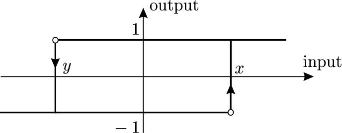
The central assumption that we make is that the switching threshold for the transition of a relay (bacterium) from state 1 to state $- 1$ is different from the switching threshold for the opposite transition (the difference of the thresholds $2 x$ is called the bi-stability range). That is, we assume hysteresis, or multi-stability, in the switching response of bacteria to the exogenous stimulus. This hysteresis can be viewed as form of the persistent memory of past environmental conditions by organisms. Since the seminal work of Max Delbrük [14], epigenetic differences arising in the process of cell differentiation have been attributed to multi-stability of living forms. A classical example of such multi-stability is the behavior of lac-operon in E. coli (lac-operon is a collection of genes associated with transport and metabolism of lactose in the bacterium; expression of these genes can be turned on by molecules called inducers). Experimental studies of the regulation of enzymes in E. coli and yeast that were conducted as early as in the 1950–1960s effectively demonstrated that two phenotypes each associated with “on” and “off” state of lac-operon expression can be obtained from the same culture. The fraction of each phenotype in the total population depended on the history of exposure to the inducer, and each phenotype remained stable through multiple generations of the bacteria [5,10,11,39,40,47,51]. This behavior resembles the two-threshold hysteretic relay shown in Fig. 1. Later, multi-stable gene expression and hysteresis have been well-documented in many natural as well as artificially constructed systems [4,15,19,41,45]. In particular, recent experiments using molecular biology methods permitted a further study of the region of bi-stability of the lac-operon when multiple input variables are used to switch the lac-operon genes on and off.

Fig. 1.

Non-ideal relay.

A substantial amount of experimental and theoretical work provides an evidence that organisms use various (often randomized) strategies of phenotype switching in order to adapt to changing environmental conditions (see [36] and references therein). It is intuitively clear that phenotypic diversity within the population can help to increase the chances of survival in varying environment. Switching strategies that establish phenotypic diversity are called bet-hedging [3]. Indeed, experimental and theoretical models of adaptation demonstrate that bet-hedging can evolve to maximize the net growth of the total population [1,2,28,38,42,48]. In [18], a simple differential model was used to show that switching strategies with two thresholds where the switching moment depends not only on the state of the environment, but also on the phenotype itself, can further increase Darwinian fitness of species. These strategies exploit hysteresis and are described by a two-threshold relay shown in Fig. 1 in the adiabatic limit when switching is faster than the characteristic rate of the environment variations. It was also shown in [18] that the optimal bi-stability range, that is the optimal separation of thresholds $2 x$ of the relay, which maximizes the net growth rate of the population is different for different environmental inputs. For this reason, the model that is considered in this work includes the distribution of bacteria (relays) over a set of switching strategies which have different separation of switching thresholds with x taking the values from an interval $[\underline{x}, \overline{x}]$ . The diffusion process included in the model acts as a factor that diversifies the switching thresholds (strategies) in the population, while the competition provides a mechanism of selection that may favor a subpopulation with a specific x for a given law of variation of the state of environment. More detailed discussion of the model assumptions and the biological background can be found in [17,18,20].

Parabolic equations with distributed non-ideal relays were previously used for modeling spatial structures that were observed in spatially distributed colonies of bacteria, for example concentric rings in Petri dish experiments [9,22,23,26,27,37]. In these models, all the relays have the same fixed separation of thresholds. The mechanism of pattern formation discussed in this work is based on the long-term memory of the hysteretic relays and is related to dynamics of free boundary separating the domain where relays are in state 1 from the domain where relays are in state $- 1$ on the interval $[\underline{x}, \overline{x}]$ . This mechanism is different from the mechanism found in [9,26,27]. Other important aspects of dynamics of parabolic and hyperbolic differential equations with distributed relays were studied in [6,8,12,16,24,25,29,30,33,49,50] in relation to multiple applied problems (not related to patterns) such as phase transitions, population dynamics, multi-phase flows in porous media, thermostat control and others.

In the following Sections 2 and 3 we present the model and a statement on its well-posedness that has been obtained earlier. Section 4 contains the main statement on the asymptotics of the patterns and its proof.

2. Model description

In this paper, we consider a class of models, which attempt to account for a number of phenomena, namely (a) switching of bacteria between two phenotypes (states) in response to variations of environmental conditions; (b) hysteretic switching strategy (switching rules) associated with bi-stability of phenotype states; (c) heterogeneity of the population in the form of a distribution of switching thresholds; (d) bet-hedging in the form of diffusion between subpopulations characterized by different bi-stability ranges; and (e) competition for nutrients. The resulting model is a reaction–diffusion system including, as reaction terms, discontinuous hysteresis relay operators and the integral of those. This integral can be interpreted as the Preisach operator [7,13,31,32,34,35,43,44,46,50] with a time dependent density (the density is a component of the solution describing the varying distribution of bacteria). In [21], we have shown that fitness, competition and diffusion can act together to select a non-trivial distribution of phenotypes (states) over the population of thresholds. The main goal of this paper is to give a quantative description of this distribution for small diffusion.

We assume that each of the two phenotypes, denoted by 1 and $- 1$ , consumes a different type of nutrient (for example, one consumes lactose and the other glucose). The amount of nutrient available for phenotype i at the moment t is denoted by $f_{i} (t)$ where $i = \pm 1$ . The model is based on the following assumptions (see [20] for further discussion).

Each bacterium changes phenotype in response to the variations of the variable $w = f_{1} / (f_{1} + f_{- 1}) - 1 / 2$ , which measures the deviation of the relative concentration of the first nutrient from the value $1 / 2$ in the mixture of the two nutrients.

The input $w = w (t)$ is mapped to the (binary) phenotype (state) of a bacterium $r (t) = R^{x} (w) (t)$ , where $R^{x}$ is the non-ideal relay operator with symmetric switching thresholds x, $y = - x$ with $x > 0$ ; see Fig. 1 and the rigorous definition (3.1) in Section 3.

The population includes bacteria with different bi-stability ranges $(- x, x)$ , where the threshold value x varies over an interval $[\underline{x}, \overline{x}] \subset (0, 1 / 2)$ . We will denote by $u (x, t)$ the density of the biomass of bacteria with given switching thresholds $\pm x$ at a moment t.

There is a diffusion process acting on the density u.

At any particular time moment t, for any given x, all the bacteria with the switching threshold values $\pm x$ are in the same state (phenotype). That is, $u (x, t)$ is the total density of bacteria with the threshold x at the moment t and they are all in the same state. This means that when a bacterium with a threshold $x^{'}$ sporadically changes its threshold to a different value x, it simultaneously copies the state from other bacteria which have the threshold x. In particular, this may require a bacterium to change the state when its threshold changes.

With these assumptions, we obtain the following model of the evolution of bacteria and nutrients, $\begin{matrix} (2.1) & \{\begin{matrix} u_{t} = D u_{x x} + \frac{1}{2} (1 + R^{x} (w)) u f_{1} + \frac{1}{2} (1 - R^{x} (w)) u f_{- 1}, \\ {\dot{f}}_{1} = - \frac{1}{2} f_{1} \int_{\underline{x}}^{\overline{x}} (1 + R^{x} (w)) u d x, \\ {\dot{f}}_{- 1} = - \frac{1}{2} f_{- 1} \int_{\underline{x}}^{\overline{x}} (1 - R^{x} (w)) u d x, \end{matrix} \end{matrix}$ where $u_{t}$ and $u_{x x}$ are the derivatives of the population density u; $D > 0$ is the diffusion coefficient; dot denotes the derivative with respect to time; and all the non-ideal relays $R^{x}$ , $x \in [\underline{x}, \overline{x}]$ , have the same input $w = f_{1} / (f_{1} + f_{- 1}) - 1 / 2$ . We additionally assume the growth rate $\frac{1}{2} (1 + i R^{x} (w)) u f_{i}$ based on the mass action law for bacteria in the phenotype $i = \pm 1$ . The rate of the consumption of nutrient in the equation for $f_{i} = f_{i} (t)$ is proportional to the total biomass of bacteria in the phenotype i, hence to the integral; $\underline{x}$ and $\overline{x}$ are the lower and upper bounds on available threshold values, respectively.

We assume that a certain amount of nutrients is available at the initial moment; the nutrients are not supplied after that moment. We assume the Neumann boundary conditions for u, that is no flux of the population density u through the lower and upper bounds of available threshold values.

3. Rigorous setting of a well-posed model

3.1. Rigorous setting

Throughout the paper, we assume that $x \in [\underline{x}, \overline{x}] \subset (0, 1 / 2)$ .

We begin with a rigorous definition of the hysteresis operator $R^{x}$ (non-ideal relay) with fixed thresholds $\pm x$ . This operator takes a continuous function $w = w (t)$ defined on an interval $t \in [0, T)$ to the binary function $r = R^{x} (w)$ of time defined on the same interval, which is given by $\begin{matrix} (3.1) & R^{x} (w) (t) = \{\begin{matrix} - 1 & if w (τ) ⩽ - x for some τ \in [0, t] and w (s) < x for all s \in [τ, t], \\ 1 & if w (τ) ⩾ x for some τ \in [0, t] and w (s) > - x for all s \in [τ, t], \\ r_{0} & if - x < w (τ) < x for all τ \in [0, t], \end{matrix} \end{matrix}$ where $r_{0}$ is either 1 or $- 1$ (initial state of the non-ideal relay $R^{x}$ ). Since $r_{0}$ may take different values for different x, we write $r_{0} = r_{0} (x)$ . The function $r_{0} = r_{0} (x)$ of $x \in [\underline{x}, \overline{x}]$ taking values $\pm 1$ is called the initial configuration of the non-ideal relays. In what follows, we do not explicitly indicate the dependence of the operator $R^{x}$ on $r_{0} (x)$ .

In this paper, we assume that $r_{0} (x)$ is simple, which means the following. There is a partition $\underline{x} = {\bar{x}}_{0} < {\bar{x}}_{1} < \dots < {\bar{x}}_{N_{0}} = \overline{x}$ of the interval $[\underline{x}, \overline{x}]$ such that the function $r_{0} (x)$ , which satisfies $| r_{0} (x) | = 1$ for all $\underline{x} ⩽ x ⩽ \overline{x}$ , is constant on each interval $({\bar{x}}_{k - 1}, {\bar{x}}_{k}]$ and has different signs on any two adjacent intervals: $\begin{matrix} (3.2) & \begin{matrix} r_{0} (x) = r_{0} ({\bar{x}}_{k}), x \in ({\bar{x}}_{k - 1}, {\bar{x}}_{k}], k = 1, \dots, N_{0}, \\ r_{0} ({\bar{x}}_{k - 1}) r_{0} ({\bar{x}}_{k}) = - 1, k = 2, \dots, N_{0}, \end{matrix} \end{matrix}$ where the second relation holds if $N_{0} ⩾ 2$ .

We define the distributed relay operator $R (w)$ taking functions $w = w (t)$ to functions $r = r (x, t)$ by $\begin{matrix} (3.3) & r (x, t) = R (w) (x, t) : = R^{x} (w) (t) . \end{matrix}$ The function $r (\cdot, t)$ will be referred to as the configuration (state) of the distributed relay operator at the moment t.

We set $\begin{matrix} (3.4) & \underline{U} (t) = \int_{\underline{x}}^{\overline{x}} u (x, t) d x, P (u, w) (t) = \int_{\underline{x}}^{\overline{x}} u (x, t) R^{x} (w) (t) d x . \end{matrix}$ Here the first integral is the total mass of bacteria; $P$ is the so-called Preisach operator with the time dependent density function u. Further, we replace the unknown functions $f_{1}$ and $f_{- 1}$ in system (2.1) by the functions $v = f_{1} + f_{- 1}$ (total mass of the two nutrients) and $w = f_{1} / (f_{1} + f_{- 1}) - 1 / 2$ (deviation of the relative concentration of the first nutrient from the value $1 / 2$ ). Substituting $\begin{matrix} f_{1} = (\frac{1}{2} + w) v, f_{- 1} = (\frac{1}{2} - w) v \end{matrix}$ into the first equation of (2.1), we obtain the equation $\begin{matrix} u_{t} = D u_{x x} + (\frac{1}{2} + w R (w)) u v . \end{matrix}$ Furthermore, summing the second and the third equations of system (2.1) and using the relationships $v = f_{1} + f_{- 1}$ , $2 w v = f_{1} - f_{- 1}$ and the notation (3.4), we get $\begin{matrix} \dot{v} = - (\frac{\underline{U}}{2} + w P (u, w)) v . \end{matrix}$ Finally, from the second and the third equations of (2.1), it follows that $\begin{matrix} \dot{w} = \frac{{\dot{f}}_{1} f_{- 1} - f_{1} {\dot{f}}_{- 1}}{{(f_{1} + f_{- 1})}^{2}} = - \frac{f_{1} f_{- 1}}{v^{2}} \int_{\underline{x}}^{\overline{x}} u R^{x} (w) d x = - (\frac{1}{2} + w) (\frac{1}{2} - w) P (u, w) . \end{matrix}$

Thus, the resulting system, which is equivalent to equations (2.1), takes the form $\begin{matrix} (3.5) & \{\begin{matrix} u_{t} = D u_{x x} + (\frac{1}{2} + w R (w)) u v, \\ \dot{v} = - (\frac{\underline{U}}{2} + w P (u, w)) v, \\ \dot{w} = - (\frac{1}{2} + w) (\frac{1}{2} - w) P (u, w), \end{matrix} \end{matrix}$ where we assume the Neumann boundary conditions $\begin{matrix} (3.6) & u_{x} |_{x = \underline{x}} = u_{x} |_{x = \overline{x}} = 0 \end{matrix}$ and the initial conditions $\begin{matrix} (3.7) & \begin{matrix} u (x, 0) = u_{0} (x), v (0) = v_{0}, w (0) = w_{0}, r (x, 0) = r_{0} (x), \\ u_{0} (x) ⩾ 0, \int_{\underline{x}}^{\overline{x}} u_{0} (x) d x = 1, v_{0} ⩾ 0, | w_{0} | ⩽ \overline{x}, r (x) is simple . \end{matrix} \end{matrix}$

3.2. Well-posedness

The problems (3.5)–(3.7), which contains a discontinuous distributed relay operator, was shown in [20] to be well posed. We briefly summarize this result before proceeding with the analysis of long time behavior.

Set $Q_{T} = (\underline{x}, \overline{x}) \times (0, T)$ for $T > 0$ . We will use the standard Lebesgue spaces $L_{2} (Q_{T})$ and $L_{2} = L_{2} (\underline{x}, \overline{x})$ ; the Sobolev spaces $W_{2}^{k} = W_{2}^{k} (\underline{x}, \overline{x})$ , $k \in N$ ; the anisotropic Sobolev space $W_{2}^{2, 1} (Q_{T})$ with the norm $\begin{matrix} ∥ u ∥_{W_{2}^{2, 1} (Q_{T})} = {(\int_{0}^{T} {∥ u (\cdot, t) ∥}_{W_{2}^{2}}^{2} d t + \int_{0}^{T} {∥ u_{t} (\cdot, t) ∥}_{L_{2}}^{2} d t)}^{1 / 2}, \end{matrix}$ and the space $\begin{matrix} W (Q_{T}) = W_{2}^{2, 1} (Q_{T}) \times C^{1} [0, T] \times C^{1} [0, T] . \end{matrix}$

Definition 3.1.
Assume that $(u_{0}, v_{0}, w_{0}) \in W_{2}^{1} \times R^{2}$ . We say that $(u, v, w)$ is a (global) solution to problems (3.5)–(3.7) if, for any $T > 0$ , $(u, v, w) \in W (Q_{T})$ , $r (\cdot, t)$ is a continuous $L_{2}$ -valued function for $t ⩾ 0$ , and relations (3.5)–(3.7) hold in the corresponding function spaces.

The following result was proved in [20].
Theorem 3.1.
If $(u_{0}, v_{0}, w_{0}) \in W_{2}^{1} \times R^{2}$ , then
Problems (3.5)–(3.7) has a unique solution $(u, v, w)$ ;

The state $r (\cdot, t) = R (w) (\cdot, t)$ of the distributed relay operator is simple for all $t ⩾ 0$ ;

We have $\begin{array}{l} (3.8) & \dot{\underline{U}} (t) ⩾ 0, \underline{U} (t) \to 1 + v_{0}, 0 ⩽ u (\cdot, t) \to \frac{1 + v_{0}}{\overline{x} - \underline{x}} in C [\underline{x}, \overline{x}], \\ (3.9) & \dot{v} (t) ⩽ 0, v (t) ⩽ v_{0} e^{- μ t} with μ = 1 / 2 - \overline{x} > 0, \\ (3.10) & | w (t) | ⩽ \overline{x} < 1 / 2, \end{array}$ where the convergence takes place as $t \to \infty$ .

The behavior given by (3.8)–(3.10) is to be expected. Indeed, as we assume no supply of nutrients after the initial moment, the total amount of nutrients $v (t)$ converges to zero. When the density of nutrients vanishes as a result of consumption by bacteria, the equation for the density u approaches the homogeneous heat equation with zero flux boundary conditions, which explains why the density of bacteria $u (x, t)$ converges to a uniform distribution over the interval $[\underline{x}, \overline{x}]$ as a result of the diffusion.

Below we are interested in the limiting behavior of the configuration function $r (x, t)$ given by (3.3), or, in other words, in the limiting distribution of phenotypes over the population of thresholds. In [21], we have proved that $r (x, t)$ converges to a step like profile as $t \to \infty$ , see Fig. 2. In the next section, we give a quantative description of this phenomenon under the assumptions that the initial amount of nutrient $v_{0}$ and the diffusion coefficient D tend to zero, while the initial density $u_{0} (x)$ tends to the delta function.

Fig. 2.
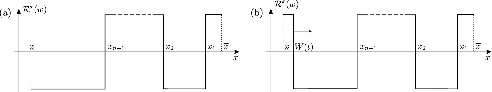
Spatial configuration of the relays $R^{x} (w)$ at a moment $t > t_{n - 1}$ . (a) The input satisfies $w (t) \in (- \overline{x} + q_{n - 1}, \underline{x})$ . Hence, the relays do not switch and all the fronts are steady. (b) The input satisfies $w (t) \in (\underline{x}, \overline{x} - q_{n})$ . Hence, the relays may switch and the nth front $W (t)$ can move.
4. Fronts asymptotics

4.1. Terminology

A point ${\bar{x}}_{j} = {\bar{x}}_{j} (t)$ which separates an interval on which the relays are in state 1 from an interval on which the relays are in state $- 1$ is called a front; cf. (3.2). The total number of fronts can vary, but, by Theorem 3.1, remains finite at all times (equivalently, the state of the distributed relay operator remains simple at all times). A front can either stay (a steady front) or move right. That is, any ${\bar{x}}_{j} (t)$ is a non-decreasing function on the time interval of its existence. A front disappears if it hits another front or is hit by another front. Assume a front ${\bar{x}}_{j} (t)$ exists at a moment $t_{0}$ . It is called immortal up to time T, $T > t_{0}$ , if it does not disappear on the time interval $t_{0} ⩽ t ⩽ T$ .

Our goal is to give asymptotic formulas for the time moments at which steady immortal (up to time T) fronts appear as well as for their positions. This will be done as $D \to 0$ , where D is the diffusion coefficient in (3.5) responsible for random fluctuations of hysteresis thresholds of individual bacteria.

4.2. Assumptions

From now on, we fix a time interval $[0, T]$ , $T > 0$ . Along with conditions (3.7), we assume that the initial density satisfies the relation $\begin{matrix} (4.1) & u_{0} (x) ⩽ ε, x \in (\underline{x}, \overline{x} - ε), \end{matrix}$ where $ε > 0$ will be chosen small enough and depending on D.

We introduce the function $\begin{matrix} (4.2) & F (x) : = 1 / 4 - {(\overline{x} - x)}^{2} \end{matrix}$ and set $\begin{array}{l} (4.3) & s_{1 / 2} : = \int_{0}^{\overline{x} + \underline{x}} \frac{d x}{F (x)}, \\ (4.4) & \overline{F} : = 2 \int_{0}^{\overline{x}} \frac{d x}{F (x)} . \end{array}$ Set $\begin{matrix} U (x, t) : = \int_{x}^{\overline{x}} u (y, t) d y, E (y) : = \frac{2}{\sqrt{π}} \int_{0}^{y} e^{- z^{2}} d z . \end{matrix}$

Using [21, Lemmas 4.1 and 5.4] and the fact that $0 ⩽ \underline{U} (t) - 1 ⩽ v_{0}$ (see (3.7) and (3.8)), we can choose positive functions $ε (D)$ and $v_{0} (D)$ such that $ε (D), v_{0} (D) \to 0$ as $D \to 0$ and $\begin{matrix} (4.5) & sup_{t \in [s_{1 / 2} / 2, T]} {∥ U (\cdot, t) - E (\frac{\overline{x} - \cdot}{2 {(D t)}^{1 / 2}}) ∥}_{C [\underline{x}, \overline{x}]} = o (1) as D \to 0, \end{matrix}$ provided that $u_{0} (x)$ satisfies (4.1) with $ε = ε (D)$ and that $v_{0} = v_{0} (D)$ .

The main assumptions will be as follows.

The initial density $u_{0} (x)$ satisfies (4.1) with $ε = ε (D)$ , where $ε (D)$ is the above function.

The initial amount of food is small: $v_{0} = v_{0} (D)$ , where $v_{0} (D)$ is the above function.

The initial value of the input is close to $\overline{x}$ : $w_{0} = w_{0} (D)$ , where $w_{0} (D)$ is an arbitrary function such that $w_{0} (D) ⩽ \overline{x}$ and $w_{0} (D) \to \overline{x}$ as $D \to 0$ .

The initial configuration is $r_{0} (x) \equiv 1$ .

Our goal is to determine the consecutive time moments $t_{n}$ at which the moving fronts become steady and their positions $x_{n}$ ( $n = 1, 2, \dots$ ) at these moments.

We begin with the following recursive algorithm for determining (finitely or infinitely many) positive numbers $\begin{matrix} (4.6) & 0 = s_{0} < s_{1} < s_{2} < \dots < s_{n} < \dots, y_{1}, y_{2}, \dots, y_{n}, \dots . \end{matrix}$

4.3. Algorithm

Basis. Set $s_{1} : = \overline{F}$ , and let $y_{1}$ be the (unique) root of the equation $2 E (y) = 1$ , $y \in (0, \infty)$ .

Set $G_{2} (t) : = - 2 E (y_{1} {(\frac{s_{1}}{t})}^{1 / 2})$ . Note that $G_{2} (s_{1}) + 1 = 0$ and ${\dot{G}}_{2} (t) > 0$ for all $t > 0$ .

Inductive conjecture. Fix $n ⩾ 2$ . Assume that we have defined the sequences $s_{1}, \dots, s_{n - 1}$ and $y_{1}, \dots, y_{n - 1}$ such that the function $\begin{matrix} (4.7) & G_{n} (t) : = 2 \sum_{j = 1}^{n - 1} {(- 1)}^{n + j} E (y_{j} {(\frac{s_{j}}{t})}^{1 / 2}) \end{matrix}$ satisfies $\begin{matrix} (4.8) & G_{n} (s_{n - 1}) + 1 = 0, G_{n} (t) + 1 > 0, t > s_{n - 1} . \end{matrix}$ As we have seen, relations (4.8) hold for $n = 2$ .

Below we will also use the equivalent recursive representation of $G_{n} (t)$ : $\begin{matrix} (4.9) & G_{1} (t) \equiv 0, G_{n} (t) = - G_{n - 1} (t) - 2 E (y_{n - 1} {(\frac{s_{n - 1}}{t})}^{1 / 2}), n ⩾ 2 . \end{matrix}$

Inductive step. Now we will determine $s_{n}$ , $y_{n}$ , and the function $G_{n + 1} (t)$ satisfying relations (4.9) with n replaced by $n + 1$ .

Consider the equation $\begin{matrix} (4.10) & \int_{s_{n - 1}}^{s} (G_{n} (t) + 1) d t = \overline{F}, s \in [s_{n - 1}, \infty) . \end{matrix}$ Due to (4.8) and the fact that $G_{n} (t) + 1 \to 1$ as $t \to \infty$ , the left-hand side is a strictly increasing function of s that tends to ∞ as $s \to \infty$ . Therefore, Eq. (4.10) has a unique root, which we denote by ${\tilde{s}}_{n}$ .

Consider the function $\begin{matrix} (4.11) & H_{n} (t, z) : = - G_{n} (t) - 2 E (\frac{z}{t^{1 / 2}}) + 1, t ⩾ {\tilde{s}}_{n}, z ⩾ 0 . \end{matrix}$ Relations (4.8) imply that $\begin{matrix} (4.12) & - G_{n} (t) + 1 < 2, t ⩾ {\tilde{s}}_{n} . \end{matrix}$ On the other hand, due to (4.9), $\begin{matrix} - G_{n} (t) + 1 = G_{n - 1} (t) + 2 E (y_{n - 1} {(\frac{s_{n - 1}}{t})}^{1 / 2}) + 1, t ⩾ {\tilde{s}}_{n}, \end{matrix}$ and, hence, $\begin{matrix} (4.13) & - G_{n} (t) + 1 > 0, t ⩾ {\tilde{s}}_{n}, \end{matrix}$ due to the inductive conjecture (see (4.8) with n replaced by $n - 1$ ).

Thus, we see that the equality $H_{n} (t, z) = 0$ uniquely defines a smooth positive function $z = Z_{n} (t)$ , $t ⩾ {\tilde{s}}_{n}$ , such that $\begin{matrix} (4.14) & H_{n} (t, z) > 0, z < Z_{n} (t), H (t, Z_{n} (t)) = 0, H_{n} (t, z) < 0, z > Z_{n} (t) . \end{matrix}$

Now we have several possibilities depending on the geometry of the curve $Z_{n} (t)$ defined by (4.14):

${\dot{Z}}_{n} (t) > 0$ for $t > {\tilde{s}}_{n}$ . In this case, we set $s_{n} : = {\tilde{s}}_{n}$ .

There is $s_{n} > {\tilde{s}}_{n}$ such that ${\dot{Z}}_{n} (t) < 0$ for $t \in ({\tilde{s}}_{n}, s_{n})$ and ${\dot{Z}}_{n} (t) > 0$ for $t > s_{n}$ .

Otherwise, we terminate the process at the finite sequences ${s_{1}, \dots, s_{n - 1}}$ and ${y_{1}, \dots, y_{n - 1}}$ .

In cases (3)(a) and (3)(b), we set

\begin{matrix} (4.15) & y_{n} : = \frac{Z_{n} (s_{n})}{s_{n}^{1 / 2}} . \end{matrix}

In these two cases, it remains to check that the function $\begin{matrix} (4.16) & G_{n + 1} (t) : = - G_{n} (t) - 2 E (y_{n} {(\frac{s_{n}}{t})}^{1 / 2}) \end{matrix}$ satisfies relations (4.8) with n replaced by $n + 1$ . This will guarantee that we can repeat the inductive step of the algorithm from Section 4.3 with n replaced by $n + 1$ .

Combining (4.16) with (4.11), (4.14) and (4.15), we have $\begin{matrix} G_{n + 1} (s_{n}) + 1 = - G_{n} (s_{n}) - 2 E (y_{n}) + 1 = H (s_{n}, Z (s_{n})) = 0 . \end{matrix}$ On the other hand, in cases (3)(a) and (3)(b), we have $Z_{n} (s_{n}) < Z_{n} (t)$ for $t > s_{n}$ . Therefore, relations (4.11), (4.15) and (4.16) imply that $\begin{matrix} G_{n + 1} (t) + 1 = H_{n} (t, Z_{n} (s_{n})) > 0, t > s_{n} . \end{matrix}$

4.4. Main result

4.4.1. Formulation of the main result

Assume that, for some $N ⩾ 1$ , we have the sequences ${s_{1}, \dots, s_{N}}$ and ${y_{1}, \dots, y_{N}}$ constructed according to the above algorithm, and assume that $s_{N} < T$ , where T was fixed in Section 4.2.

Theorem 4.1.
For all $n = 1, \dots, N$ , the nth moving front becomes steady and immortal (up to time $s_{N}$ ) at a moment $\begin{matrix} (4.17) & t_{n} = s_{n} + o (1) \end{matrix}$ and its position at this moment is $\begin{matrix} (4.18) & x_{n} = \overline{x} - q_{n}, where q_{n} = 2 (y_{n} + o (1)) {(D s_{n})}^{1 / 2}; \end{matrix}$ here $o (1)$ stands for functions of D that tend to 0 as $D \to 0$ . Furthermore, $x_{N} < x_{N - 1} < \dots < x_{1} < \overline{x}$ .

4.4.2. Preliminary discussion

In Section 5, we will prove Theorem 4.1. Assume we have constructed $n - 1$ fronts that became steady at the moments $t_{1}, \dots, t_{n - 1}$ at the positions $x_{1}, \dots, x_{n - 1}$ given by (4.17) and (4.18), respectively. We will consider the formation of the nth front on the time interval $[t_{n - 1}, t_{n}]$ . We consider the case of an even $n ⩾ 2$ . The case of odd n is analogous; see also Remark 5.1 below concerning $n = 1$ .

Below we will consecutively consider time moments $\begin{matrix} \begin{matrix} [t_{n - 1} = s_{n - 1} + o (1)] & < r_{n - 1} < t_{n - 1 / 2} \\ < [{\tilde{τ}}_{n} = {\tilde{s}}_{n} + o (1)] ⩽ [τ_{n} = s_{n} + o (1)] \\ ⩽ [θ_{n} = s_{n} + o (1)] ⩽ [t_{n} = s_{n} + o (1)] < r_{n} \end{matrix} \end{matrix}$ which are characterized by the following properties:

The function $w (t)$ is increasing and the relays do not switch during the time interval $t \in (t_{n - 1}, t_{n - 1 / 2})$ ; furthermore, $\begin{matrix} (4.19) & w (t_{n - 1}) = - \overline{x} + q_{n - 1}, w (t_{n - 1 / 2}) = \underline{x} . \end{matrix}$

The function $w (t)$ is increasing and some relays switch during the time interval $(t_{n - 1 / 2}, {\tilde{τ}}_{n})$ ; further, for some $Z_{*} (D) = o (1)$ (which will be chosen below to satisfy relations (5.15)), we have $\begin{matrix} (4.20) & w ({\tilde{τ}}_{n}) = \overline{x} - 2 Z_{*} (D) . \end{matrix}$ Note that, although the distance between $w ({\tilde{τ}}_{n})$ and $\overline{x}$ is already $2 Z_{*} (D) = o (1)$ , it is still much larger than the desired distance $2 (y_{n} + o (1)) {(D s_{n})}^{1 / 2}$ due to (5.12). Also the moment ${\tilde{τ}}_{n}$ , which is of order ${\tilde{s}}_{n}$ , may be much smaller than the desired moment, which is of order $s_{n}$ .

The function $w (t)$ may oscillate and the relays may, though not necessarily, switch during the time interval $({\tilde{τ}}_{n}, τ_{n})$ . The moment $τ_{n} = s_{n} + o (1)$ is already of the correct order, but the value $w (τ_{n})$ may still have a wrong asymptotics. However, it satisfies $\begin{matrix} (4.21) & w ({\tilde{τ}}_{n}) ⩽ w (τ_{n}) ⩽ \overline{x} - 2 (y_{n} + o (1)) {(D s_{n})}^{1 / 2}, \end{matrix}$ i.e., it is bounded from above by the correct asymptotics.

The function $w (t)$ may oscillate and the relays may, though not necessarily, switch during the time interval $(τ_{n}, θ_{n})$ . The moment $θ_{n} = s_{n} + o (1)$ is of the same (correct) order as $τ_{n}$ , but now, additionally, the value $w (θ_{n})$ has the correct asymptotics $\begin{matrix} (4.22) & w (θ_{n}) = \overline{x} - 2 (y_{n} + o (1)) {(D s_{n})}^{1 / 2} . \end{matrix}$

The function $w (t)$ may oscillate and the relays may, though not necessarily, switch during the time interval $(θ_{n}, t_{n})$ . The moment $t_{n} = s_{n} + o (1)$ is of the same (correct) order as $τ_{n}$ and $θ_{n}$ , and the function $w (t)$ does not oscillate any more after the moment $t_{n}$ . More precisely, $w (t)$ is decreasing and the relays do not switch during the time interval $(t_{n}, r_{n}]$ . Moreover, the nth immortal front is formed at the moment $t_{n}$ in the sense that $\begin{matrix} (4.23) & w (t_{n}) = \overline{x} - q_{n} = x_{n}, \dot{w} (t_{n}) = 0 . \end{matrix}$

5. Proof of the main result

In this section, we will prove Theorem 4.1. Recall that, without loss of generality, we assume that n is even. In Sections 5.1–5.5, we will consider in detail the respective time intervals from items (1)–(5) of Section 4.4.2.

5.1. Dynamics for $w \in (- \overline{x} + q_{n - 1}, \underline{x})$ as $t \in (t_{n - 1}, t_{n - 1 / 2})$

We will see below that $w (t)$ is increasing for $t > t_{n - 1}$ and achieves the value $w (t) = \underline{x}$ . Let $t_{n - 1 / 2}$ be the moment when this happens: $w (t_{n - 1 / 2}) = \underline{x}$ . Note that if $w (t) \in (- \overline{x} + q_{n - 1}, \underline{x})$ and $\dot{w} (t) > 0$ , then the relays do not switch.

Assume we have proved at the previous step (for n replaced by $n - 1$ ) that $\begin{matrix} (5.1) & \dot{w} (t) > 0 for t \in (t_{n - 1}, r_{n - 1}] \end{matrix}$ for some $r_{n - 1} > s_{n - 1}$ not depending on D (we shall do this for $k = n$ in the end; see (5.33)). As long as $\dot{w} (t)$ remains positive and $w (t) < \underline{x}$ holds, the relays do not switch, see Fig. 2(a). Hence, using (4.5) and (4.18), we can write the third equation in (3.5) as follows (we omit “ $u (x, t) d x$ ” for brevity): $\begin{matrix} (5.2) & \begin{matrix} \dot{w} (t) & = - (\frac{1}{4} - w^{2}) (- \int_{\underline{x}}^{x_{n - 1}} + \int_{x_{n - 1}}^{x_{n - 2}} - \int_{x_{n - 2}}^{x_{n - 3}} + \dots + \int_{x_{1}}^{\overline{x}}) \\ = (\frac{1}{4} - w^{2}) (U (\underline{x}, t) - 2 U (x_{n - 1}, t) + 2 U (x_{n - 2}, t) - \dots - 2 U (x_{1}, t)) \\ = (\frac{1}{4} - w^{2}) (1 + 2 \sum_{j = 1}^{n - 1} {(- 1)}^{j} E ((y_{j} + o (1)) {(\frac{s_{j}}{t})}^{1 / 2}) + o (1)), t > t_{n - 1} \end{matrix} \end{matrix}$ (here and below, we consider $t ⩽ T$ only).

We set $\begin{matrix} p (t) : = \overline{x} + w (t) . \end{matrix}$ Taking into account (5.2), definition (4.2) of $F (x)$ , definition (4.7) of $G_{n} (t)$ , and the fact that n is even, we see that $p (t)$ satisfies $\begin{array}{l} (5.3) & \dot{p} (t) = F (p) (G_{n} (t) + 1 + μ (t, D)), t > t_{n - 1}, \\ (5.4) & p (t_{n - 1}) = 2 (y_{n - 1} + o (1)) {(D s_{n - 1})}^{1 / 2}, \end{array}$ where $\begin{matrix} (5.5) & sup_{t \in [s_{1 / 2} / 2, T]} | μ (t, D) | ⩽ ε_{n} = ε_{n} (D) for a non-negative ε_{n} (D) = o (1) . \end{matrix}$

Due to (4.8) and (5.5), the right-hand side in (5.3) is positive for $t \in [r_{n - 1}, T]$ , provided D is small enough. Together with (5.1), this means that the solution to (5.3), (5.4) increases until a moment $t_{n - 1 / 2}$ (if it exists) at which it achieves the value $\overline{x} + \underline{x}$ . This proves that (5.3) is equivalent to the third equation in (3.5) not only for $t \in (t_{n - 1}, r_{n - 1})$ but actually for $t \in (t_{n - 1}, t_{n - 1 / 2})$ .

The following lemma determines the time moment $t_{n - 1 / 2}$ .

Lemma 5.1.
The equation $\begin{matrix} (5.6) & \int_{s_{n - 1}}^{s} (G_{n} (t) + 1) d t = \int_{0}^{\overline{x} + \underline{x}} \frac{d x}{F (x)} \end{matrix}$ has a unique root on the interval $s \in (s_{n - 1}, \infty)$ . Denote it by $s_{n - 1 / 2}$ . Then $t_{n - 1 / 2} = s_{n - 1 / 2} + o (1)$ and $\dot{p} (t_{n - 1 / 2}) > 0$ .
Proof.
Due to (4.8) and the fact that $G_{n} (t) + 1 \to 1$ as $t \to \infty$ , Eq. (5.6) has a unique root $s_{n - 1 / 2}$ .

To prove the asymptotics for $t_{n - 1 / 2}$ , we denote by $p_{\pm} (t)$ the solutions of $\begin{matrix} {\dot{p}}_{\pm} (t) = F (p_{\pm}) (G_{n} (t) + 1 \pm ε_{n}), t > t_{n - 1}, \end{matrix}$ with the same initial data at $t = t_{n - 1}$ as in (5.4). Obviously, $\begin{matrix} (5.7) & p_{-} (t) ⩽ p (t) ⩽ p_{+} (t) . \end{matrix}$

Let $t_{n - 1 / 2, \pm}$ be the first moment at which $p_{\pm} (t) = \overline{x} + \underline{x}$ . Then, integrating the differential equation for $p_{\pm} (t)$ , we obtain $\begin{matrix} \int_{s_{n - 1} + o (1)}^{t_{n - 1 / 2, \pm}} (G_{n} (t) + 1 \pm ε_{n}) d t = \int_{o (1)}^{\overline{x} + \underline{x}} \frac{d x}{F (x)} . \end{matrix}$ Using the implicit function theorem in a neighborhood of the point $(t_{n - 1 / 2, \pm}, D) = (s_{n - 1 / 2}, 0)$ , we obtain $t_{n - 1 / 2, \pm} = s_{n - 1 / 2} + o (1)$ . Therefore, taking into account (5.7), we have $t_{n - 1 / 2} = s_{n - 1 / 2} + o (1)$ .

The inequality $\dot{p} (t_{n - 1 / 2}) > 0$ has been proved before the lemma. □

5.2. Dynamics for $w \in (\underline{x}, \overline{x} - q_{n})$ as $t \in (t_{n - 1 / 2}, {\tilde{τ}}_{n})$

By Lemma 5.1, $\dot{w} (t_{n - 1 / 2}) > 0$ . Therefore, as long as $\dot{w} (t)$ remains positive, the input $w (t)$ increases and hence switches the relays. However, if $\dot{w} (t)$ becomes negative, the relays will stop switching. To describe the dynamics of $w (t)$ , we introduce the function $\begin{matrix} W (t) : = max_{s \in [t_{n - 1 / 2}, t]} w (s), \end{matrix}$ where $t_{n - 1 / 2}$ is defined in Lemma 5.1, see Fig. 2(b). Then, similarly to (5.2), we obtain from the third equation in (3.5) and from relation (4.5) $\begin{array}{rcl} \dot{w} (t) = - (\frac{1}{4} - w^{2}) (\int_{\underline{x}}^{W (t)} - \int_{W (t)}^{x_{n - 1}} + \int_{x_{n - 1}}^{x_{n - 2}} - \int_{x_{n - 2}}^{x_{n - 3}} + \dots + \int_{x_{1}}^{\overline{x}}) \\ = - (\frac{1}{4} - w^{2}) (1 - 2 U (W, t) + 2 U (x_{n - 1}, t) - 2 U (x_{n - 2}, t) + \dots + 2 U (x_{1}, t)) \\ = - (\frac{1}{4} - w^{2}) (1 - 2 E (\frac{\overline{x} - W}{2 {(D t)}^{1 / 2}}) - 2 \sum_{j = 1}^{n - 1} {(- 1)}^{j} E ((y_{j} + o (1)) {(\frac{s_{j}}{t})}^{1 / 2}) + o (1)), \\ t > t_{n - 1 / 2} . \end{array}$ Setting $\begin{matrix} q (t) : = \overline{x} - w (t), Q (t) : = min_{s \in [t_{n - 1 / 2}, t]} q (s) = \overline{x} - W (t), \end{matrix}$ we have $\begin{matrix} (5.8) & \dot{q} (t) = F (q) (- G_{n} (t) - 2 E (\frac{Q}{2 {(D t)}^{1 / 2}}) + 1 + μ (t, D)), t > t_{n - 1 / 2}, \end{matrix}$ where $\begin{matrix} (5.9) & sup_{t \in [s_{1 / 2} / 2, T]} | μ (t, D) | \to 0 as D \to 0 \end{matrix}$ with $s_{1 / 2}$ defined in (4.3). We consider Eq. (5.8) with the initial condition $\begin{matrix} (5.10) & q (t_{n - 1 / 2}) = \overline{x} - \underline{x} . \end{matrix}$ We begin with the following observation, which shows that the $(n - 1)$ th front is immortal.

Lemma 5.2.
The solution $q (t)$ to problem (5.8) , (5.10) cannot achieve the value $q_{n - 1}$ .
Proof.
Assume, by contradiction, that $q (t)$ achieves the value $q_{n - 1}$ ( $= 2 (y_{n - 1} + o (1)) {(D s_{n - 1})}^{1 / 2}$ ) for the first time at some moment $t = t^{}$ ( $> t_{n - 1 / 2} > s_{n - 2}$ ). At this moment $Q (t^{}) = q (t^{}) = q_{n - 1}$ . Since $t^{} > s_{n - 2}$ , it follows from (4.8) (with n replaced by $n - 1$ ) that $G_{n - 1} (t^{}) + 1 > 0$ . Therefore, using (5.8) and (4.9), we have $\begin{matrix} \dot{q} (t^{}) = F (0) (G_{n - 1} (t^{}) + 1) + o (1) > 0 \end{matrix}$ for all sufficiently small D, which is impossible. □

To proceed, we will need a specific (positive) function $Z_{} (D)$ such that $\begin{array}{l} (5.11) & Z_{} (D) \to 0 as D \to 0, \\ (5.12) & \frac{Z_{} (D)}{D^{1 / 2}} \to \infty as D \to 0 . \end{array}$ To define it, we introduce the new function $z (t) : = \frac{q (t)}{2 D^{1 / 2}}$ and set $\begin{matrix} (5.13) & Z (t) : = min_{s \in [t_{n - 1 / 2}, t]} z (s) . \end{matrix}$ Then we consider Eq. (5.8) for $t > {\tilde{s}}_{n}$ , where ${\tilde{s}}_{n}$ is the time moment defined in the inductive step (1) of the algorithm from Section 4.3. For such t, it is equivalent to $\begin{matrix} (5.14) & \dot{z} (t) = \frac{F (0) (H_{n} (t, Z) + o (1))}{2 D^{1 / 2}}, \end{matrix}$ where $H (t, \cdot)$ is given by (4.11). We choose the desired $Z_{} (D)$ to satisfy, for all $t \in [{\tilde{s}}_{n}, T]$ , $\begin{matrix} (5.15) & \begin{matrix} H_{n} (t, ζ) + o (1) > 0 for ζ ⩽ Z_{n} (t) - Z_{} (D), \\ H_{n} (t, ζ) + o (1) < 0 for ζ ⩾ Z_{n} (t) + Z_{} (D), \\ F (0) | H_{n} (t, ζ) + o (1) | ⩽ 2 h_{n} Z_{} (D) for ζ \in [Z_{n} (t) - Z_{} (D), Z_{n} (t) + Z_{} (D)], \end{matrix} \end{matrix}$ where $o (1)$ is the same function as in (5.14) and $h_{n} > 0$ does not depend on t and D. This can be done because $\partial H_{n} (t, Z_{n} (t)) / \partial ζ \neq 0$ for all $t \in [{\tilde{s}}_{n}, T]$ .

The following lemma defines a time moment ${\tilde{τ}}_{n}$ satisfying (4.20). Lemma 5.3.
There is a time moment ${\tilde{τ}}_{n} = {\tilde{s}}_{n} + o (1)$ such that $\dot{q} (t) < 0$ for all $t \in [t_{n - 1 / 2}, {\tilde{τ}}_{n}]$ and $q ({\tilde{τ}}_{n}) = 2 Z_{} (D)$ .
Proof.
As long as $\dot{q} (t) < 0$ and $Z_{} (D) ⩽ q (t) ⩽ \overline{x} - \underline{x}$ , we have $Q (t) = q (t)$ . Therefore, we can rewrite Eq. (5.8) as follows: $\begin{matrix} (5.16) & \dot{q} (t) = - F (q) (G_{n} (t) + 1 + μ_{1} (t, q, D)), t > t_{n - 1 / 2}, \end{matrix}$ where, due to (5.9) and (5.12), $\begin{matrix} (5.17) & sup_{q \in [0, \overline{x} - \underline{x}]} sup_{t \in [s_{1 / 2} / 2, T]} | μ_{1} (t, q, D) | ⩽ δ = δ (D) for a non-negative δ (D) = o (1) . \end{matrix}$

Due to (4.8) and (5.17), the right-hand side in (5.16) is negative for $t \in [t_{n - 1 / 2}, T]$ , provided D is small enough. Hence, $\dot{q} (t) < 0$ for $t > t_{n - 1 / 2}$ .

Denote by $q_{\pm} (t)$ the solution to the equation $\begin{matrix} (5.18) & {\dot{q}}_{\pm} (t) = - F (q_{\pm}) (G_{n} (t) + 1 \pm δ), t > t_{n - 1 / 2}, \end{matrix}$ with the same initial condition as in (5.10), $q (t_{n - 1 / 2}) = \overline{x} - \underline{x}$ .

Then, we have $q_{-} (t) ⩽ q (t) ⩽ q_{+} (t)$ . Therefore, it suffices to show that $q_{\pm} (t)$ achieves the value $2 D^{1 / 2 - λ}$ for the first time at a moment ${\tilde{τ}}_{\pm} = {\tilde{s}}_{n} + o (1)$ . Equation (5.18) yields $\begin{matrix} \int_{s_{n - 1 / 2} + o (1)}^{{\tilde{τ}}_{\pm}} (G_{n} (t) + 1 \pm δ) d t = \int_{2 Z_{*} (D)}^{\overline{x} - \underline{x}} \frac{d x}{F (x)} . \end{matrix}$

Using the fact that ${\tilde{s}}_{n}$ is a root of (4.10) and $s_{n - 1 / 2}$ is a root of (5.6) as well as the definition of $\overline{F}$ in (4.4) and the symmetry of $F (x)$ , we have $\begin{matrix} \begin{matrix} \int_{s_{n - 1 / 2}}^{{\tilde{s}}_{n}} (G_{n} (t) + 1) d t & = \int_{s_{n - 1}}^{{\tilde{s}}_{n}} (G_{n} (t) + 1) d t - \int_{s_{n - 1}}^{s_{n - 1 / 2}} (G_{n} (t) + 1) d t \\ = \overline{F} - \int_{0}^{\overline{x} + \underline{x}} \frac{d x}{F (x)} = \int_{0}^{\overline{x} - \underline{x}} \frac{d x}{F (x)} . \end{matrix} \end{matrix}$ Hence, the implicit function theorem in a neighborhood of $({\tilde{τ}}_{\pm}, D) = ({\tilde{s}}_{n}, 0)$ together with (5.11) yield ${\tilde{τ}}_{\pm} = {\tilde{s}}_{n} + o (1)$ . □

5.3. Dynamics for $w \in (\underline{x}, \overline{x} - q_{n})$ as $t \in ({\tilde{τ}}_{n}, τ_{n})$

Assume that case (3)(b) in the inductive step of the algorithm from Section 4.3 holds with some $s_{n} > {\tilde{s}}_{n}$ . If case (3)(a) holds, we omit this step and proceed with Section 5.4.

Fig. 3.

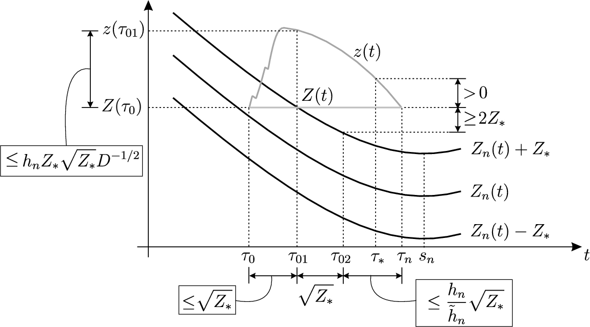
Dynamics for t close to $s_{n}$ . Three black curves are the graphs of $Z_{n} (t)$ and $Z_{n} (t) \pm Z_{*}$ . The upper grey curve is the graph of the solution $z (t)$ to Eq. (5.14). The lower (horizontal) grey curve is the graph of $Z (t)$ given by (5.13).

The following lemma defines a time moment $τ_{n}$ satisfying (4.21).

Lemma 5.4.

There is a time moment $τ_{n} = s_{n} + o (1) ⩽ s_{n}$ such that $\dot{q} (τ_{n}) < 0$ and $\begin{matrix} (5.19) & 2 (Z_{n} (τ_{n}) - Z_{*} (D)) D^{1 / 2} ⩽ q (τ_{n}) = Q (τ_{n}) ⩽ 2 Z_{*} (D) . \end{matrix}$

Proof.

To follow the proof, we refer the reader to Fig. 3. We consider Eq. (5.14) with the initial data $\begin{matrix} (5.20) & z ({\tilde{τ}}_{n}) = Z_{*} (D) D^{- 1 / 2} . \end{matrix}$ First, note that $z (t) ⩾ Z (t) > Z_{n} (t) - Z_{*} (D)$ for all $t \in [{\tilde{τ}}_{n}, s_{n}]$ . Indeed, if the equality $Z (t) = Z_{n} (t) - Z_{*} (D)$ is achieved for the first time at some moment $t \in [{\tilde{τ}}_{n}, s_{n}]$ , then $z (t) = Z (t) = Z_{n} (t) - Z_{*} (D)$ . Moreover, since $Z_{n} (t) - Z_{*} (D)$ is non-increasing, we have $\dot{z} (t) ⩽ 0$ at this moment. On the other hand, relations (5.14) and (5.15) imply that $\dot{z} (t) > 0$ . Thus, the first inequality in (5.19) holds with $τ_{n}$ replaced by any $t ⩽ s_{n}$ .

Furthermore, $Z (t)$ is non-increasing. Hence, $Z (t) ⩽ Z ({\tilde{τ}}_{n}) ⩽ Z_{*} (D) D^{- 1 / 2}$ for all $t ⩾ {\tilde{τ}}_{n}$ by Lemma 5.3. It remains to find $τ_{n}$ such that $z (τ_{n}) = Z (τ_{n})$ and $\dot{q} (τ_{n}) < 0$ .

Next, we introduce a positive function $a_{*} (D)$ such that $a_{*} (D) \to 0$ and $\begin{matrix} (5.21) & {\dot{Z}}_{n} (t) ⩽ - 2 \sqrt{Z_{*} (D)}, t ⩽ s_{n} - a_{*} (D) . \end{matrix}$ Consider the time moment $\begin{matrix} τ_{*} = τ_{*} (D) := s_{n} - a_{*} (D) - \sqrt[4]{Z_{*} (D)} . \end{matrix}$ First, assume that $\begin{matrix} (5.22) & z (τ_{*}) > Z (τ_{*}) \end{matrix}$ (the case $z (τ_{*}) = Z (τ_{*})$ will be considered at the end of the proof). Denote by $τ_{0}$ the time moment preceding $τ_{*}$ such that $\begin{matrix} (5.23) & z (τ_{0}) = Z (τ_{0}), z (t) > Z (t) = Z (τ_{0}), t \in [τ_{0}, τ_{*}] . \end{matrix}$ Obviously, $Z (τ_{0}) \in [Z_{n} (τ_{0}) - Z_{*}, Z_{n} (τ_{0}) + Z_{*}]$ . Indeed, otherwise, $Z (τ_{0}) > Z_{n} (τ_{0}) + Z_{*}$ and, due to (5.15) and Eq. (5.14), we would have $\dot{z} (τ_{0}) < 0$ .

Note that, due to (5.21), we have $Z (τ_{0}) ⩾ Z_{n} (τ_{0} + \sqrt{Z_{*}}) + Z_{*}$ . Denote by $\begin{matrix} τ_{01} \in [τ_{0}, τ_{0} + \sqrt{Z_{*}}] \end{matrix}$ a moment such that $\begin{matrix} (5.24) & Z (τ_{0}) = Z_{n} (τ_{01}) + Z_{*} . \end{matrix}$ If $Z (τ_{01}) < Z (τ_{0})$ , then there exists a desired time moment $τ_{n} \in [τ_{0}, τ_{01}]$ and the proof is complete.

Assume that $Z (τ_{01}) = Z (τ_{0})$ . Then (5.24) yields $\begin{matrix} (5.25) & Z (τ_{01}) = Z_{n} (τ_{01}) + Z_{*} . \end{matrix}$

Let us estimate the velocity $\dot{z} (t)$ for $t \in [τ_{0}, τ_{01}]$ . For such t, we have $Z (t) ⩾ Z_{n} (t) - Z_{*}$ and, due to (5.24), $Z (t) = Z (τ_{0}) ⩽ Z_{n} (t) + Z_{*}$ . Hence, (5.15) implies that $\dot{z} (t) ⩽ h_{n} Z_{*} D^{- 1 / 2}$ for $t \in [τ_{0}, τ_{01}]$ . Therefore, $\begin{matrix} (5.26) & z (τ_{01}) ⩽ Z (τ_{0}) + h_{n} Z_{*} \sqrt{Z_{*}} D^{- 1 / 2} . \end{matrix}$

Set $\begin{matrix} τ_{02} := τ_{01} + \sqrt{Z_{*}} . \end{matrix}$ From $\dot{Z} (t) < 0$ it follows that $Z (t) > Z_{n} (t) + Z_{*}$ for $t \in [τ_{01}, τ_{02}]$ . If $Z (τ_{02}) < Z (τ_{01})$ , then there exists a desired time moment $τ_{n} \in [τ_{01}, τ_{02}]$ and the proof is complete.

Assume that $Z (τ_{02}) = Z (τ_{01})$ . It follows from (5.21) and (5.25) that $\begin{matrix} (5.27) & Z (τ_{02}) = Z (τ_{01}) = Z_{n} (τ_{01}) + Z_{*} ⩾ Z_{n} (τ_{02}) + Z_{*} + 2 Z_{*} . \end{matrix}$ Furthermore, due to (5.15) and Eq. (5.14), we have $\begin{matrix} \dot{z} (t) < 0, t \in [τ_{01}, τ_{02}] . \end{matrix}$ Therefore (see (5.26)), $\begin{matrix} (5.28) & z (τ_{02}) ⩽ z (τ_{01}) ⩽ Z (τ_{0}) + h_{n} Z_{*} \sqrt{Z_{*}} D^{- 1 / 2} . \end{matrix}$

Now inequality (5.27), relations (5.15) and Eq. (5.14) imply that $\dot{z} (t) ⩽ - {\tilde{h}}_{n} Z_{*} D^{- 1 / 2}$ at least as long as $z (t) ⩾ Z (τ_{02}) = Z (τ_{0})$ , where ${\tilde{h}}_{n}$ does not depend on t and D. Therefore, taking into account (5.28), we see that $z (t)$ will achieve the value $Z (τ_{02}) = Z (τ_{0})$ at a time moment $τ_{n} \in [τ_{02}, τ_{02} + h_{n} \sqrt{Z_{*}} / {\tilde{h}}_{n}]$ . If follows from (5.23) and from the definitions of $τ_{*}$ , $τ_{0}$ , $τ_{01}$ , $τ_{02}$ and $τ_{n}$ that $τ_{n} \in (τ_{*}, s_{n})$ . Hence, $τ_{n}$ is the desired time moment.

Finally, if (5.22) is not valid, then $z (τ_{*}) = Z (τ_{*})$ and, as we already know, $Z (τ_{*}) ⩽ Z_{*} D^{- 1 / 2}$ . The equality $z (τ_{*}) = Z (τ_{*})$ implies $\dot{q} (τ_{*}) ⩽ 0$ . If $\dot{q} (τ_{*}) < 0$ , then we can choose $τ_{n} = τ_{*}$ . If $\dot{q} (τ_{*}) = 0$ , then relations (5.14), (5.15) imply $Z (τ_{*}) \in [Z_{n} (τ_{*}) - Z_{*}, Z_{n} (τ_{*}) + Z_{*}]$ and all the argument following Eq. (5.23) can be repeated for $τ_{0} = τ_{*}$ . □

5.4. Dynamics for

w \in (\underline{x}, \overline{x} - q_{n})

t \in (τ_{n}, θ_{n})

Lemma 5.5.
There is a time moment $θ_{n} = τ_{n} + o (1)$ such that $\dot{q} (t) < 0$ for $t \in [τ_{n}, θ_{n}]$ and $q (θ_{n}) = 2 (y_{n} + o (1)) {(D s_{n})}^{1 / 2}$ .
Proof.
Setting $z (t) = \frac{q (t)}{2 D^{1 / 2}}$ , we consider the problem (see Lemma 5.4) $\begin{matrix} (5.29) & \{\begin{matrix} \dot{z} (t) = \frac{F (0) (H (t, Z (t)) + o (1))}{2 D^{1 / 2}}, \\ y_{n} s_{n}^{1 / 2} - Z_{} (D) ⩽ z (τ_{n}) ⩽ Z_{} D^{- 1 / 2}, \end{matrix} \end{matrix}$ where $H (t, z)$ is given by (4.11). If $z (τ_{n}) ⩽ Z_{n} (τ_{n}) + Z_{} (D) = y_{n} s_{n}^{1 / 2} + Z_{} (D) + o (1)$ , then we take $θ_{n} := τ_{n}$ and complete the proof.

Assume that $z (τ_{n}) > Z_{n} (τ_{n}) + Z_{} (D)$ . We need to prove that there exist positive functions $ε_{} (D)$ and $δ_{} (D)$ that tend to zero as $D \to 0$ and such that the solution $z (t)$ to (5.14) satisfies $\begin{matrix} \dot{z} (t) < 0, t \in [τ_{n}, τ_{n} + δ_{} (D)], y_{n} ⩽ z (τ_{n} + δ_{} (D)) ⩽ (y_{n} + ε_{} (D)) s_{n}^{1 / 2} . \end{matrix}$

To construct the functions $ε_{} (D)$ and $δ_{} (D)$ , we consider positive sequences $ε_{k}, δ_{k} \to 0$ such that $δ_{k} ⩽ s_{n} / 2$ . Due to (4.13), (4.14) and (4.15), there exists a sequence $c_{k} = c_{k} (ε_{k})$ such that $\begin{matrix} (5.30) & H (t, z) ⩽ - c_{k}, t \in [{\tilde{s}}_{n}, T], z ⩾ Z_{n} (t) + ε_{k} . \end{matrix}$ Then (5.29) and (5.30) imply that $z (t)$ achieves the value $Z_{n} (t) + ε_{k}$ at a time moment $θ_{n k}$ that satisfies $\begin{matrix} 0 ⩽ θ_{n k} - τ_{n} ⩽ \frac{Z_{} (D) D^{- 1 / 2}}{{inf}_{t \in [\tilde{s}, 2 s_{n}]} | \dot{z} (t) |} ⩽ \frac{4 Z_{} (D)}{F (0) c_{k}} ⩽ δ_{k} \end{matrix}$ for all $D ⩽ D_{k}$ , where $D_{k}$ is a strictly decreasing sequence with $D_{k} \to 0$ . Therefore, $z (θ_{n k}) = Z_{n} (θ_{n k}) + ε_{k} = (y_{n} + {\tilde{ε}}_{k}) s_{n}^{1 / 2}$ where ${\tilde{ε}}_{k} \to 0$ as $k \to \infty$ . Now we set $ε_{} (D) := {\tilde{ε}}_{k}$ and $δ_{} (D) := δ_{k}$ for $D \in (D_{k}, D_{k - 1}]$ . □
5.5. Dynamics for $w \in (\underline{x}, \overline{x} - q_{n})$ as $t \in (θ_{n}, t_{n})$

To describe the dynamics for $t > θ_{n}$ , we consider (5.8) with the initial data $\begin{matrix} (5.31) & q (θ_{n}) = 2 (y_{n} + o (1)) {(D s_{n})}^{1 / 2} \end{matrix}$ (see Lemma 5.5). The following lemma will allow us to justify (5.1) (with $n - 1$ replaced by n) and thus to complete the proof of Theorem 4.1.

Lemma 5.6.
There exists ${\tilde{θ}}_{n} = s_{n} + o (1) ⩾ θ_{n}$ and $r_{n}$ ( $> s_{n}$ ) not depending on D such that the solution $q (t)$ to (5.8) , (5.31) satisfies $\dot{q} (t) > 0$ for $t \in [{\tilde{θ}}_{n}, r_{n}]$ and $w (r_{n}) > - \underline{x}$ .
Proof.
Since $F (q) ⩾ 1 / 4 - {\overline{x}}^{2}$ for $q \in [0, \overline{x} - \underline{x}]$ , it suffices to estimate the expression in brackets in (5.8). Using the definition of $Q (t)$ , the monotonicity of $E (\cdot)$ , and relations (5.31) and (4.8) (with $n - 1$ replaced by n), we see that there exists ${\tilde{θ}}_{n} = s_{n} + o (1) ⩾ θ_{n}$ such that $\begin{matrix} (5.32) & \begin{matrix} - G_{n} (t) - 2 E (\frac{Q (t)}{2 {(D t)}^{1 / 2}}) + 1 + μ (t, D) \\ ⩾ - G_{n} (t) - 2 E (\frac{q (θ_{n})}{2 {(D t)}^{1 / 2}}) + 1 + μ (t, D) \\ = G_{n + 1} (t) + 1 + o (1) > 0 for t ⩾ {\tilde{θ}}_{n} . \end{matrix} \end{matrix}$

Equation (5.8) and inequality (5.32) imply that $\dot{q} (t) > 0$ for $t ⩾ {\tilde{θ}}_{n}$ . Obviously, we can choose $r_{n} > s_{n}$ independent of D such that $w (r_{n}) = \overline{x} - q (r_{n}) > - \underline{x}$ . □

Finally, we determine the time moment $t_{n}$ (see (4.23)) at which the nth front becomes steady and immortal and its position $x_{n} = \overline{x} - q_{n}$ as follows: $\begin{matrix} t_{n} := sup {t \in [θ_{n}, {\tilde{θ}}_{n}] : \dot{q} (t) = 0, q (t) = Q (t)}, q_{n} := q (t_{n}) = Q (t_{n}) . \end{matrix}$ Due to Lemmas 5.5 and 5.6, $t_{n} = s_{n} + o (1)$ and $\begin{matrix} (5.33) & \dot{q} (t) > 0 for t \in (t_{n}, r_{n}] . \end{matrix}$ This justifies (5.1) (with $n - 1$ replaced by n). Moreover, since $\dot{q} (t_{n}) = 0$ , the value $y := \frac{Q (t_{n})}{2 {(D t_{n})}^{1 / 2}}$ satisfies (due to (5.8) and (5.9)) $\begin{matrix} 0 = - G_{n} (s_{n} + o (1)) - 2 E (y) + 1 + o (1) . \end{matrix}$ On the other hand, the definition (4.11) of $H_{n} (t, z)$ , the definition (4.14) of $Z_{n} (t)$ and the definition (4.15) of $y_{n}$ imply that $y_{n}$ is the root of the equation $\begin{matrix} 0 = - G_{n} (s_{n}) - 2 E (y_{n}) + 1 . \end{matrix}$ Therefore, $y = y_{n} + o (1)$ , which implies $q (t_{n}) = Q (t_{n}) = 2 (y_{n} + o (1)) {(D s_{n})}^{1 / 2}$ . This completes the proof of Theorem 4.1. Remark 5.1.
An essential ingredient in the proof is the approximation (4.5) of the integral of the solution U by the error function $E (\cdot)$ . It is valid for t separated from zero and thus can be used for $n ⩾ 2$ . In the case $n = 1$ , the analog of Eq. (5.3) will be $\dot{q} (t) = f (q) \underline{U} (t)$ on the interval $t \in (0, t_{1 / 2})$ , where $q (t) = \overline{x} - w (t)$ , $q (0) = o (1)$ and $q (t_{1 / 2}) = \overline{x} + \underline{x}$ . On this time interval, one can use the approximation $\underline{U} (t) = 1 + o (1)$ (see (3.7) and (3.8)) instead of (4.5).

6. Numerics

Fig. 4.

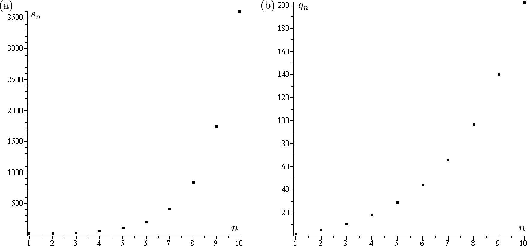
The two graphs indicate the values of (a) $s_{n}$ and (b) $q_{n}$ for $n = 1, \dots, 10$ from Theorem 4.1. The maximal and minimal values for admissible thresholds are $\underline{x} = 1 / 100$ and $\overline{x} = 1 / 4$ , respectively.

Figure 4 illustrates the values of $s_{n}$ and $q_{n}$ for $n = 1, \dots, 10$ from Theorem 4.1 found numerically. We note that ${\tilde{s}}_{n} = s_{n}$ for $n = 1, \dots, 6$ (i.e., case (3)(a) from the inductive step of the algorithm from Section 4.3 takes place) and ${\tilde{s}}_{n} < s_{n}$ for $n = 7, \dots, 10$ (i.e., case (3)(b) from the inductive step takes place). In general, it is an open question whether one of the two cases (3)(a) and (3)(b) takes place for all n, or both may fail for some n and hence the resulting sequences (4.6) are finite.

Footnotes

Acknowledgements

Pavel Gurevich acknowledges the support of the DFG through the Collaborative Research Center 910 and the Heisenberg fellowship. Dmitrii Rachinskii was supported by National Science Foundation, Grant DMS-1413223. The authors are grateful to Sergey Tikhomirov who created a software for a number of numerical experiments.

References

[1]

Acar,

Becskei and

van Oudenaarden, Enhancement of cellular memory by reducing stochastic transitions, Nature 435 (2005), 228–232.

[2]

Acar,

J.T.

Mettetal and

van Oudenaarden, Stochastic switching as a survival strategy in fluctuating environments, Nature Genetics 40(4) (2008), 471–475.

[3]

H.J.E.

Beaumont,

Gallie,

Kost,

G.C.

Ferguson and

P.B.

Rainey, Experimental evolution of bet hedging, Nature 462 (2009), 90–93.

[4]

Becskei,

Seraphin and

Serrano, Positive feedback in eukaryotic gene networks: Cell differentiation by graded to binary response conversion, EMBO J. 20 (2001), 2528–2535.

[5]

Benzer, Induced synthesis of enzymes in bacteria analyzed at the cellular level, Biochim. Biophys. Acta 11(3) (1953), 383–395.

[6]

Brokate,

N.D.

Botkin and

O.A.

Pykhteev, Numerical simulation for a two-phase porous medium flow problem with rate independent hysteresis, Physica B: Condensed Matter 407(9) (2012), 1336–1339.

[7]

Brokate,

Pokrovskii and

Rachinskii, Asymptotic stability of continuum sets of periodic solutions to systems with hysteresis, J. Math. Anal. Appl. 319 (2006), 94–109.

[8]

Brokate and

Sprekels, Hysteresis and Phase Transitions, Springer, 1996.

[9]

Chiu,

F.C.

Hoppensteadt and

Jäger, Analysis and computer simulation of accretion patterns in bacterial cultures, J. Math. Biol. 32 (1994), 841–855.

10.

[10]

Cohn and

Horbita, Inhibition by glucose of the induced synthesis of the beta-galactoside-enzyme system of Escherichia coli. Analysis of maintenance, J. Bacteriol. 78 (1959), 601–612.

11.

[11]

Cohn and

Horbita, Analysis of the differentiation and of the heterogeneity within a population of Escherichia coli undergoing induced beta-galactosidase synthesis, J. Bacteriol. 78 (1959), 613–623.

12.

[12]

Colli,

Grasselli and

Sprekels, Automatic control via thermostats of a hyperbolic Stefan problem with memory, Appl. Math. Optim. 39 (1999), 229–255.

13.

[13]

Cross,

McNamara,

Pokrovskii and

Rachinskii, A new paradigm for modelling hysteresis in macroeconomic flows, Physica B 403(2,3) (2008), 231–236.

14.

[14]

Delbrück, Discussion, in: Unités Biologiques Douées de Continuité Génétique, Editions du Centre National de la Recherche Scientifique, Paris, 1949, pp. 33–35.

15.

[15]

Dubnau and

Losick, Bistability in bacteria, Mol. Microbiol. 61 (2006), 564–572.

16.

[16]

Friedman and

L.-S.

Jiang, Periodic solutions for a thermostat control problem, Commun. Partial Differ. Equ. 13(5) (1988), 515–550.

17.

[17]

Friedman,

Gurevich,

McCarthy and

Rachinskii, Switching behaviour of two-phenotype bacteria in varying environment, J. Phys.: Conf. Ser. 585 (2015), 0121012.

18.

[18]

Friedman,

McCarthy and

Rachinskii, Hysteresis can grant fitness in stochastically varying environment, PLoS ONE 9(7) (2014), e103241.

19.

[19]

T.S.

Gardner,

C.R.

Cantor and

J.J.

Collins, Construction of a genetic toggle switch in Escherichia coli, Nature 403 (2000), 339–342.

20.

[20]

Gurevich and

Rachinskii, Well-posedness of parabolic equations containing hysteresis with diffusive thresholds, Tr. Mat. Inst. Steklova 283 (2013), 92–114; English transl.: Proc. Steklov Inst. Math.283 (2013), 87–109.

21.

[21]

Gurevich and

Rachinskii, Pattern formation in parabolic equations containing hysteresis with diffusive thresholds, J. Math. Anal. Appl. 424 (2015), 1103–1124.

22.

[22]

Gurevich and

Tikhomirov, Uniqueness of transverse solutions for reaction–diffusion equations with spatially distributed hysteresis, Nonlinear Anal. A: Theory, Methods and Applications 75 (2012), 6610–6619.

23.

[23]

Gurevich and

Tikhomirov, Systems of reaction–diffusion equations with spatially distributed hysteresis, Mathematica Bohemica 139(2) (2014), 239–257.

24.

[24]

P.L.

Gurevich, Periodic solutions of parabolic problems with hysteresis on the boundary, Discrete Cont. Dynam. Systems A 29(3) (2011), 1041–1083.

25.

[25]

P.L.

Gurevich and

S.B.

Tikhomirov, Symmetric periodic solutions of parabolic problems with discontinuous hysteresis, J. Dynamics and Differential Equations 23(4) (2011), 923–960.

26.

[26]

F.C.

Hoppensteadt and

Jäger, Pattern formation by bacteria, in: Biological Growth and Spread, Lecture Notes in Biomathematics, Vol. 38, Springer, 1980, pp. 68–81.

27.

[27]

F.C.

Hoppensteadt,

Jäger and

Pöppe, A hysteresis model for bacterial growth patterns, in: Modelling of Patterns in Space and Time, Lecture Notes in Biomathematics, Vol. 55, Springer, 1984, pp. 123–134.

28.

[28]

B.B.

Kaufmann,

Yang,

J.T.

Mettetal and

van Oudenaarden, Heritable stochastic switching revealed by single-cell genealogy, PLoS Biol. 5(9) (2007), e239.

29.

[29]

Kopfová, Hysteresis in biological models, J. Phys.: Conf. Ser. 55 (2006), 130–134.

30.

[30]

Kopfová and

Aiki, A mathematical model for bacterial growth, in: Recent Advances in Nonlinear Analysis, Proceedings of the International Conference on Nonlinear Analysis, World Scientific, 2008, pp. 1–10.

31.

[31]

Krasnosel’skii and

Rachinskii, On continua of cycles in systems with hysteresis, Doklady Math. 63(3) (2001), 339–344.

32.

[32]

Krasnosel’skii and

Rachinskii, On a bifurcation governed by hysteresis nonlinearity, NoDEA Nonlinear Differential Equations Appl. 9 (2002), 93–115.

33.

[33]

Krejčí, Hysteresis, Convexity and Dissipation in Hyperbolic Equations, GAKUTO International Series: Mathematical Sciences and Applications, Vol. 8, Gakkotosho, Tokyo, 1996.

34.

[34]

Krejci,

O’Kane,

Pokrovskii and

Rachinskii, Stability results for a soil model with singular hysteretic hydrology, J. Phys.: Conf. Ser. 268(1) (2011), 012016.

35.

[35]

Krejci,

O’Kane,

Pokrovskii and

Rachinskii, Properties of solutions to a class of differential models incorporating Preisach hysteresis operator, Physica D 241 (2012), 2010–2028.

36.

[36]

Kussell and

Lieber, Phenotypic diversity, population growth, and information in fluctuating environments, Science 309 (2005), 2075–2078.

37.

[37]

Mimura,

Sakaguchi and

Matsushita, Reaction–diffusion modelling of bacterial colony patterns, Physica A 282 (2000), 283–303.

38.

[38]

H.D.

Møller,

K.S.

Andersen and

Regenberg, A model for generating several adaptive phenotypes from a single genetic event Saccharomyces cerevisiae GAP1 as a potential bet-hedging switch, Commun. Integr. Biol. 6(3) (2013), e23933.

39.

[39]

Monod, From enzymatic adaptation to allosteric transitions, Science 154 (1966), 475–483.

40.

[40]

Novick and

Weiner, Enzyme induction as an all-or-none phenomenon, Proc. Natl. Acad. Sci. USA 43 (1957), 553–566.

41.

[41]

E.M.

Ozbudak,

Thattai,

H.N.

Lim,

B.I.

Shraiman and

van Oudenaarden, Multistability in the lactose utilization network of Escherichia coli, Nature 427 (2004), 737–740.

42.

[42]

V.R.

Pannala,

P.J.

Bhat,

Bhartiya and

K.V.

Venkatesh, Systems biology of GAL regulon in Saccharomyces cerevisiae, WIREs Syst. Biol. Med. 2(1) (2010), 98–106.

43.

[43]

Pimenov,

Kelly,

Korobeinikov,

M.J.A.

O’Callaghan,

Pokrovskii and

Rachinskii, Memory effects in population dynamics: Spread of infectious disease as a case study, Mathematical Modelling of Natural Phenomena 7(1) (2012), 1–30.

44.

[44]

Pimenov and

Rachinskii, Linear stability analysis of systems with Preisach memory, Discrete Cont. Dynam. Systems B 11(4) (2009), 997–1018.

45.

[45]

J.R.

Pomerening,

E.D.

Sontag and

J.E.

FerrellJr., Building a cell cycle oscillator: Hysteresis and bistability in the activation of Cdc2, Nature Cell Biol. 5 (2003), 346–351.

46.

[46]

Rachinskii, Asymptotic stability of large-amplitude oscillations in systems with hysteresis, NoDEA Nonlinear Differential Equations Appl. 6(3) (1999), 267–288.

47.

[47]

Spiegelman and

W.F.

DeLorenzo, Substrate stabilization of enzyme-forming capacity during the segregation of a heterozygote, Proc. Natl. Acad. Sci. USA 38(7) (1952), 583–592.

48.

[48]

Thattai and

van Oudenaarden, Stochastic gene expression in fluctuating environments, Genetics 167 (2004), 523–530.

49.

[49]

Visintin, Evolution problems with hysteresis in the source term, SIAM J. Math. Anal. 17 (1986), 1113–1138.

50.

[50]

Visintin, Differential Models of Hysteresis, Springer, Berlin, Heidelberg, 1994.

51.

[51]

Ö.

Winge and

Roberts, Inheritance of enzymatic characters in yeasts, and the phenomenon of long-term adaptation, Compt. Rend. Lab. Carlsberg, Sér. Physiol. 24 (1948), 263–315.

Asymptotics of sign-changing patterns in hysteretic systems with diffusive thresholds

Abstract

Keywords

1. Introduction

3. Rigorous setting of a well-posed model

3.1. Rigorous setting

3.2. Well-posedness

4.1. Terminology

4.2. Assumptions

4.3. Algorithm

4.4. Main result

4.4.1. Formulation of the main result

5. Proof of the main result

5.1. Dynamics for w ∈ ( − x ‾ + q n − 1 , x _ ) as t ∈ ( t n − 1 , t n − 1 / 2 )

Footnotes

Acknowledgements

References

5.1. Dynamics for $w \in (- \overline{x} + q_{n - 1}, \underline{x})$ as $t \in (t_{n - 1}, t_{n - 1 / 2})$