Corrector estimates for a class of imperfect transmission problems

Abstract

Based on previous homogenization results for imperfect transmission problems in two-component domains with periodic microstructure, we derive quantitative estimates for the difference between the microscopic and macroscopic solution. This difference is of order $ε^{ρ}$ , where $ε > 0$ describes the periodicity of the microstructure and $ρ \in (0, \frac{1}{2}]$ depends on the transmission condition at the interface between the two components. The corrector estimates are proved without assuming additional regularity for the local correctors using the periodic unfolding method.

Keywords

Homogenization corrector results error estimates periodic unfolding two-component domain periodic interface imperfect transmission

1. Introduction

This paper considers a class of linear elliptic equations with an imperfect transmission condition modeling, for instance, heat conduction, diffusion, or stationary current flow in a composite material. The macroscopic domain Ω consists of a connected component $Ω_{1}^{ε}$ and a second component $Ω_{2}^{ε}$ , which is the collection of periodically distributed inclusions or pores. The characteristic length scale of the microstructure, given by the distance between two such pores, is of order ε. On the interface $Γ^{ε}$ between the two components, the flux is proportional to the jump of the solution across this interface, which models e.g. a contact resistance. The corresponding proportionality factor is of order $ε^{γ}$ with $γ \in R$ . More precisely, we consider for $ε > 0$ the problem $\begin{matrix} (1.1) & \begin{array}{l} - div (A^{ε} \nabla u_{1}^{ε}) = f in Ω_{1}^{ε}, \\ - div (A^{ε} \nabla u_{2}^{ε}) = f in Ω_{2}^{ε}, \\ A^{ε} \nabla u_{1}^{ε} \cdot n_{1}^{ε} = - A^{ε} \nabla u_{2}^{ε} \cdot n_{2}^{ε} on Γ^{ε}, \\ - A^{ε} \nabla u_{1}^{ε} \cdot n_{1}^{ε} = ε^{γ} h^{ε} (u_{1}^{ε} - u_{2}^{ε}) on Γ^{ε}, \\ u_{1}^{ε} = 0 on \partial Ω, \end{array} \end{matrix}$ where $n_{i}^{ε}$ is the unit outer normal to $Ω_{i}^{ε}$ for $i = 1, 2$ . The matrix $A^{ε} (x) \in R_{sym}^{d \times d}$ and the coefficient $h^{ε} (x)$ are ε-periodic and uniformly bounded. Moreover, we suppose that $A^{ε}$ is uniformly elliptic, $h^{ε}$ is strictly positive, and the source term f is square-integrable.

For ε tending to zero, the homogenization limit of problem (1.1) has already been well studied in the literature. Based on Tartar’s method for oscillating test functions, the homogenization limit was derived for all $γ ⩽ 1$ in [11,26]; see references therein for earlier works. This problem was also treated for two connected components [3], poly crystals [21], for stochastic microstructures [20], and evolution problems [8,22]. Recently, the homogenization limit and strong two-scale convergence of the gradients were proved in [10] for $γ ⩽ 1$ via the method of periodic unfolding. However, up to now all publications contain qualitative results, whereas, this paper provides quantitative corrector estimates.

In the limit $ε \to 0$ , we obtain one homogenized elliptic equation posed in the whole macroscopic domain $\begin{array}{l} (1.2) & \begin{array}{l} - div (A_{γ}^{0} \nabla u) = f in Ω, \\ u = 0 on \partial Ω . \end{array} \end{array}$ The constant matrix $A_{γ}^{0} \in R_{sym}^{d \times d}$ depends on γ, whereby we distinguish the following three cases: (i) for $- 1 < γ ⩽ 1$ , (ii) for $γ = - 1$ , and (iii) for $γ < - 1$ . The case $γ > 1$ is not treated here, since it allows for unbounded solutions as it is shown in [21].

For $γ < - 1$ , the jump $u_{1}^{ε} - u_{2}^{ε}$ across the interface $Γ^{ε}$ is negligibly small such that $A_{γ}^{0}$ is given via the standard unit cell problem on the whole reference cell, see (6.2) for more details. In other words, the model in (1.1) behaves for $ε ≪ 1$ like a classical Poisson equation with ε-periodic coefficients in a one-component domain.

For $γ = - 1$ , the matrix $A_{- 1}^{0}$ is obtained by solving a unit cell problem in two sub-domains of the reference cell separated by an interface, see (5.2). In this case, the unit cell problem reflects the structure of (1.1) on the level of the reference cell and the effective matrix takes the imperfect transmission condition into account. Indeed, this is the only case, where the effective matrix depends on the values of the boundary term $h^{ε}$ .

For $- 1 < γ ⩽ 1$ , we obtain the same effective matrix $A_{γ}^{0}$ as in [7], cf. (4.2), wherein the homogenization of the Poisson equation is considered in the perforated domain $Ω_{1}^{ε}$ with no-flux boundary conditions at the holes. In their situation, the function f is multiplied by the ratio of the volume of the occupied domain $Ω_{1}^{ε}$ divided by the total volume of Ω. However, this ratio does not appear in (1.2) which shows that the exchange between the two components is sufficient in order to take into account also the source term in $Ω_{2}^{ε}$ .

The main result of this paper are the quantitative error estimates between the microscopic solution $(u_{1}^{ε}, u_{2}^{ε})$ , the macroscopic limit u, and their corresponding correctors for the three different cases: (i) in the Theorems 4.1 and 4.3, (ii) in Theorem 5.1, and (iii) in Theorem 6.3. In the special case $γ = 1$ , the jump across the interface $Γ^{ε}$ is of order $O (1)$ and it depends on $f, h^{ε}$ , and the volume fraction of the component $Ω_{2}^{ε}$ . To prove this result in Theorem 4.3, we require additional $H^{2}$ -regularity for the source term f and that $h^{ε}$ is constant. In the case $γ < - 1$ , Lipschitz continuity of the matrix $A^{ε}$ is assumed for technical reasons.

For all $γ ⩽ 1$ , the $L^{2}$ -corrector estimates are of order $ε^{ρ (γ)}$ with $0 < ρ (γ) ⩽ 1 / 2$ , and in the special cases $γ \in {- 1, 0, 1}$ or $γ ⩽ - 2$ we recover the maximal convergence rate $ρ = 1 / 2$ . In order to prove these quantitative estimates, we need that the limit u is of higher $H^{2}$ -regularity, whereas $u_{1}^{ε}$ and $u_{2}^{ε}$ as well as the local correctors are in general only $H^{1}$ -regular. The derivation of the corrector estimates relies on the two-scale formulation of the limit (1.2) as in [10], the periodic unfolding method as in [4,5], and unfolding based error estimates as in [15,16,28]. The key step of the proofs is to construct the correct approximating sequences via defining suitable recovery operators. Those operators recover the oscillations of the gradients in the components $Ω_{1}^{ε}$ and $Ω_{2}^{ε}$ from the macroscopic limit and the local correctors. Especially for the case (i), the new operator $H_{2}^{ε}$ is introduced in (3.6) in order to capture the “flatness” of the gradient $\nabla u_{2}^{ε}$ within the inclusions.

The text is structured as follows. In Section 2, we present the model as well as all necessary assumptions and notations. In Section 3, the periodic unfolding method is introduced and we define the unfolding and folding (averaging) operator and, in particular, the recovery operators in Section 3.1. In the case (i), the corrector estimates are given in Section 4. Therein, we distinguish the cases $- 1 < γ < 1$ (Theorem 4.1) and $γ = 1$ (Theorem 4.3) in the Sections 4.1 and 4.2, respectively, although they share the same effective matrix. The remaining corrector estimates for the cases (ii) and (iii) are given in the Sections 5, and 6, respectively. We conclude the presentation with a brief discussion in Section 7 and a possible application to supercapacitors in Section 7.1.

Fig. 1.

The two-component domain Ω (left) and the reference cell Y (right).

2. The imperfect transmission problem posed in a two-component domain

Throughout the text we postulate the following assumptions on the domain and the periodic microstructure as shown in Fig. 1.

The macroscopic domain Ω is a d-dimensional polytope with $d ⩾ 2$ , i.e. it is $\begin{array}{l} Ω = \prod_{i = 1}^{d} [a_{i}, b_{i}) with a_{i} < b_{i} and a_{i}, b_{i} \in Z . \end{array}$

The reference cell ${Y = [0, 1)}^{d}$ is the disjoint union of the subsets $Y_{1}$ and $\overline{Y_{2}}$ , where $Y_{2} \subset Y$ is open, connected, and satisfies $dist (Y_{2}, \partial Y) > 0$ . The inner boundary $Γ = \partial Y_{2}$ is Lipschitz continuous and it holds $Y_{1} = Y ∖ \overline{Y_{2}}$ .

Let $K_{ε} = {λ \in Z^{d} ∣ ε λ \in Ω}$ denote the set of nodal points inside Ω. The two disjoint components $Ω_{1}^{ε}$ and $Ω_{2}^{ε}$ , and their common boundary $Γ^{ε}$ are given via $\begin{array}{l} Ω_{1}^{ε} = ⋃_{λ \in K_{ε}} ε (λ + Y_{1}), Ω_{2}^{ε} = ⋃_{λ \in K_{ε}} ε (λ + Y_{2}), and Γ^{ε} = \partial Ω_{2}^{ε} . \end{array}$

The microscopic period $ε > 0$ is given via $ε = 1 / n$ with $n \in N$ such that Ω is the exact union of translated cells $ε (λ + Y)$ with $λ \in K_{ε}$ for all ε.

By construction, the set

Ω_{1}^{ε}

is connected, bounded, and has a Lipschitz boundary, whereas the set

Ω_{2}^{ε}

consists of isolated inclusions. The former implies the existence of extension operators mapping from

H_{D}^{1} (Ω_{1}^{ε})

H_{D}^{1} (Ω)

, where the subscript D indicates homogeneous Dirichlet boundary conditions. Indeed,

\partial Ω_{1}^{ε}

is the disjoint union of

Γ^{ε}

and

\partial Ω

, and it is

\begin{array}{l} H_{D}^{1} (Ω_{1}^{ε}) = {u \in H^{1} (Ω_{1}^{ε}) ∣ u = 0 on \partial Ω} . \end{array}

The assumption that

Y_{2}

does not touch the boundary of the reference cell Y is essential for the construction of the recovery operator

H_{2}^{ε}

in (3.6), see Remark 3.1. This assumption is also contained in [10].

Remark 2.1.
The Assumption (D4) significantly simplifies the presentation of the corrector estimates, however, the results remain valid for arbitrary domains Ω with smooth boundary and $ε \in R$ . In such a case, one considers bigger domains ${\tilde{Ω}}_{i}^{ε}$ , $i = 1, 2$ , satisfying again (D2)–(D4) and uses Lemma A.6 to control the error at the boundary (cf. [15,16,28]). In any case, we have to avoid cells $ε (λ + Y)$ intersecting the boundary $\partial Ω$ such that $Ω_{1}^{ε}$ is always a Lipschitz domain (cf. also [10, Fig. 2]).

In order to obtain unique and bounded solutions for the microscopic respective homogenized problem, we require the following assumptions for the given data. The dot “ $\cdot$ ” always denotes the scalar product in $R^{d}$ .
The matrix $A \in L^{\infty} (Y; R_{sym}^{d \times d})$ is Y-periodic, symmetric, and uniformly elliptic, i.e. $\begin{array}{l} \exists α > 0 : A (y) ξ \cdot ξ ⩾ α | ξ |^{2} for all ξ \in R^{d}, and a.a. y \in Y . \end{array}$

The boundary term h is a Y-periodic function in $L^{\infty} (Γ)$ and satisfies $\begin{array}{l} \exists h_{0} > 0 : h (y) ⩾ h_{0} for a.a. y \in Γ . \end{array}$

It is $f \in L^{2} (Ω)$ and the coefficients of the microscopic problem are given via $\begin{array}{l} A^{ε} (x) = A (\frac{x}{ε}) and h^{ε} (x) = h (\frac{x}{ε}) . \end{array}$
Under the above assumptions, the Lax–Milgram theorem yields the existence of a unique solution $(u_{1}^{ε}, u_{2}^{ε})$ for the weak formulation of the microscopic problem (1.1) (cf. [26, Section 1]), i.e. find $(u_{1}^{ε}, u_{2}^{ε}) \in H_{D}^{1} (Ω_{1}^{ε}) \times H^{1} (Ω_{2}^{ε})$ such that $\begin{array}{l} \int_{Ω_{1}^{ε}} A^{ε} \nabla u_{1}^{ε} \cdot \nabla φ_{1} d x + \int_{Ω_{2}^{ε}} A^{ε} \nabla u_{2}^{ε} \cdot \nabla φ_{2} d x + ε^{γ} \int_{Γ^{ε}} h^{ε} (u_{1}^{ε} - u_{2}^{ε}) (φ_{1} - φ_{2}) d σ_{x} \\ (2.1) & = \int_{Ω_{1}^{ε}} f φ_{1} d x + \int_{Ω_{2}^{ε}} f φ_{2} d x \end{array}$ for all admissible test functions $(φ_{1}, φ_{2}) \in H_{D}^{1} (Ω_{1}^{ε}) \times H^{1} (Ω_{2}^{ε})$ . Moreover, this solution satisfies the following a priori bounds.
Proposition 2.2 ([26, Prop. 3.1]).

Any solution of the microscopic problem ( 1.1 ) is bounded for all $γ ⩽ 1$ via $\begin{array}{l} {‖ u_{1}^{ε} ‖}_{H^{1} (Ω_{1}^{ε})} + {‖ \nabla u_{2}^{ε} ‖}_{L^{2} (Ω_{2}^{ε})} + ε^{\frac{γ}{2}} {‖ u_{1}^{ε} - u_{2}^{ε} ‖}_{L^{2} (Γ^{ε})} ⩽ C, \end{array}$ where the constant $C > 0$ is independent of ε.

The solution $u \in H_{D}^{1} (Ω)$ of the homogenized problem (1.2) is unique and bounded, too. Moreover, u is of higher regularity, since the macroscopic domain Ω is a bounded convex polytope. Indeed, it holds according to [18, Thm. 3.2.1.3] $\begin{array}{l} ‖ u ‖_{H^{2} (Ω)} ⩽ C ‖ f ‖_{L^{2} (Ω)}, \end{array}$ where $C > 0$ only depends on the effective matrix $A_{γ}^{0} \in R_{sym}^{d \times d}$ and the domain Ω. The precise definition of $A_{γ}^{0}$ depends on the three different regimes (i)–(iii) for γ and it is given in the corresponding section.

3. Periodic unfolding

Following [4 ,6,10], we define the periodic unfolding operators $T_{1}^{ε}$ and $T_{2}^{ε}$ , which map one-scale functions on the oscillating domains $Ω_{1}^{ε}$ and $Ω_{2}^{ε}$ to two-scale functions on the fixed domains $Ω \times Y_{1}$ and $Ω \times Y_{2}$ , respectively. Therefore, let $x = [x] + {x}$ denote the standard two-scale decomposition of every $x \in R^{d}$ into its integer part $[x] \in Z^{d}$ and the remainder ${x} : = x - [x] \in Y$ . For any Lebesgue measurable function u on $Ω_{1}^{ε}$ the periodic unfolding operator $T_{1}^{ε}$ is given via $\begin{array}{l} (T_{1}^{ε} u) (x, y) : = u (ε [\frac{x}{ε}] + ε y) for a.a. (x, y) \in Ω \times Y_{1} \end{array}$ and it satisfies the integration formula $\begin{array}{l} (3.1) & \int_{Ω_{1}^{ε}} u d x = \int_{Ω \times Y_{1}} T_{1}^{ε} u d x d y for u \in L^{1} (Ω_{1}^{ε}) . \end{array}$ Within the inclusions, we define for any Lebesgue measurable function u on $Ω_{2}^{ε}$ the second periodic unfolding operator $T_{2}^{ε}$ by (cf. [10, Def. 2.8]) $\begin{array}{l} (T_{2}^{ε} u) (x, y) : = u (ε [\frac{x}{ε}] + ε y) for a.a. (x, y) \in Ω \times Y_{2} . \end{array}$ In particular, both periodic unfolding operators are well-defined for functions u on Ω via the relation $T_{i}^{ε} u = T_{i}^{ε} (χ_{Ω_{i}^{ε}} u)$ , for $i = 1, 2$ , with $χ_{Ω_{i}^{ε}}$ denoting the characteristic function of the set $Ω_{i}^{ε}$ . Moreover, the restriction of $T_{i}^{ε}$ to Lebesgue measurable functions u on $Γ^{ε}$ is also well-defined and it is $T_{1}^{ε} u = T_{2}^{ε} u$ almost everywhere in $Ω \times Γ$ . We recall that for Sobolev functions $u_{i} \in W^{1, p} (Ω_{i}^{ε})$ the unfolding $T_{i}^{ε} u_{i}$ belongs to the space $L^{p} (Ω; W^{1, p} (Y_{i}))$ , for all $1 ⩽ p ⩽ \infty$ and $i = 1, 2$ . Then, if the traces of $u_{1}$ and $u_{2}$ coincide in $L^{p} (Γ^{ε})$ , so do the traces of $T_{1}^{ε} u_{1}$ and $T_{2}^{ε} u_{2}$ in $L^{p} (Ω \times Γ)$ . There holds the following integration formula for boundary unfolding (cf. [6, Prop. 5.2]) $\begin{array}{l} (3.2) & ε \int_{Γ^{ε}} u d σ_{x} = \int_{Ω \times Γ} T_{1}^{ε} u d x d σ_{y} = \int_{Ω \times Γ} T_{2}^{ε} u d x d σ_{y} for u \in L^{1} (Γ^{ε}) . \end{array}$ We complete this collection by introducing the folding operator (sometimes called averaging operator) $F_{i}^{ε} : L^{p} (Ω \times Y_{i}) \to L^{p} (Ω_{i}^{ε})$ 1

¹
Note that $L^{p} (Ω \times Y)$ and $L^{p} (Ω; L^{p} (Y))$ can be identified for $1 ⩽ p < \infty$ , whereas this fails for $p = \infty$ .

for

i = 1, 2

and

1 ⩽ p < \infty

via

\begin{array}{l} (F_{i}^{ε} U) (x) : = ⨏_{ε ([\frac{x}{ε}] + Y)} U (z, {\frac{x}{ε}}) d z for a.a. x \in Ω_{i}^{ε}, \end{array}

where

⨏_{O} = | O |^{- 1} \int_{O}

denotes the usual average over the domain

O \subset R^{d}

. Here, and in the following,

| O |

denotes the d-dimensional Lebesgue measure of domains respective the

d - 1

-dimensional Lebesgue measure of hypersurfaces.

According to [4,10], the folding operator $F_{1}^{ε}$ is the adjoint of $T_{1}^{ε}$ , i.e. $\begin{array}{l} \int_{Ω_{1}^{ε}} (F_{1}^{ε} U) v d x = \int_{Ω \times Y_{1}} U (T_{1}^{ε} v) d x d y for U \in L^{2} (Ω \times Y_{1}), v \in L^{2} (Ω_{1}^{ε}) . \end{array}$ In the same manner, $F_{2}^{ε}$ is the adjoint of $T_{2}^{ε}$ . Finally, we note that the periodic unfolding respective averaging operator, $T_{ε}$ and $F_{ε}$ , as introduced in [5] are given via $\begin{array}{l} T_{ε} u = \{\begin{matrix} T_{1}^{ε} u & in Ω \times Y_{1} \\ T_{2}^{ε} u & in Ω \times Y_{2} \end{matrix} and F_{ε} U = \{\begin{matrix} F_{1}^{ε} (U |_{Ω \times Y_{1}}) & in Ω_{1}^{ε} \\ F_{2}^{ε} (U |_{Ω \times Y_{2}}) & in Ω_{2}^{ε} . \end{matrix} \end{array}$

3.1. Construction of recovery operators

In this section we introduce two operators, $G_{ε}$ and $H_{2}^{ε}$ , which will help us to construct suitable recovery respective approximating sequences for the derivation of the corrector estimates. To do so, we define the scale-splitting operator $Q_{ε} : H^{1} (Ω) \to W^{1, \infty} (R^{d})$ following [5, Def. 4.1]. Let $\tilde{u} \in H^{1} (R^{d})$ denote the extension of $u \in H^{1} (Ω)$ according to [27, Thm. 3.9]. For $x \in ε ([x / ε] + Y)$ and every $κ = (κ_{1}, \dots, κ_{d}) \in {0, 1}^{d}$ , we set $\begin{array}{l} {\bar{x}}_{l}^{(κ_{l})} : = \{\begin{matrix} \frac{x_{l} - ε {[x / ε]}_{l}}{ε} & if κ_{l} = 1 \\ 1 - \frac{x_{l} - ε {[x / ε]}_{l}}{ε} & if κ_{l} = 0 \end{matrix} \end{array}$ and $\begin{array}{l} (Q_{ε} u) (x) : = \sum_{κ \in {0, 1}^{d}} (F_{ε} \tilde{u}) (ε [\frac{x}{ε}] + ε κ) \cdot {\bar{x}}_{1}^{(κ_{1})} \dots {\bar{x}}_{d}^{(κ_{d})} . \end{array}$ The function $Q_{ε} u$ interpolates the values of $F_{ε} u$ at the nodes $ε [x / ε]$ via $Q_{1}$ -Lagrange elements as customary in the finite elements methods. Since $Q_{ε} u$ is (weakly) differentiable, in contrast to $F_{ε} u$ , we can use the scale-splitting operator to construct oscillating one-scale functions that recover global corrector-type functions $\hat{u} (x, y) = \sum_{i = 1}^{d} \frac{\partial u}{\partial x_{i}} (x) \cdot χ_{i} (y)$ . Let $H_{per}^{1} (Y)$ respective $H_{per}^{1} (Y_{1})$ denote the space of Y-periodic Sobolev functions, i.e. $\begin{array}{l} H_{per}^{1} (Y_{1}) = {φ \in H^{1} (Y_{1}) ∣ φ is Y -periodic} . \end{array}$ For any Y-periodic function, we may identify $x \mapsto φ (x)$ with $x \mapsto φ ({x})$ for all $x \in R^{d}$ .

For $u \in H^{2} (Ω)$ and $χ \in H_{per}^{1} {(Y)}^{d} : = H_{per}^{1} (Y; R^{d})$ , the approximating sequence ${(G_{ε} \hat{u})}_{ε} \subset H_{D}^{1} (Ω)$ is given via (cf. [15]) $\begin{array}{l} (3.3) & (G_{ε} \hat{u}) (x) : = ϱ_{ε} (x) \sum_{i = 1}^{d} Q_{ε} (\frac{\partial u}{\partial x_{i}}) (x) \cdot χ_{i} (\frac{x}{ε}) . \end{array}$ The cut-off function $ϱ_{ε} \in C_{c}^{\infty} (Ω; [0, 1])$ satisfies $ϱ_{ε} (x) \equiv 1$ for all $x \in Ω$ with $dist (x, \partial Ω) > ε$ and $| \nabla ϱ_{ε} | ⩽ \frac{c_{0}}{ε}$ ; and it guarantees the Dirichlet boundary condition on $\partial Ω$ . We may also call $G_{ε} : (H^{2} (Ω), H_{per}^{1} {(Y)}^{d}) \to H_{D}^{1} (Ω)$ recovery respective gradient folding operator, since it holds $T_{ε} (G_{ε} \hat{u}) \to \hat{u}$ and $T_{ε} [ε \nabla (G_{ε} \hat{u})] \to \nabla_{y} \hat{u}$ in $L^{2} (Ω \times Y)$ . The uniform boundedness of the scale-splitting operator $‖ Q_{ε} u ‖_{H^{1} (Ω)} ⩽ C ‖ u ‖_{H^{1} (Ω)}$ according to [5, Prop. 4.5] implies the following bound $\begin{array}{l} ‖ G_{ε} \hat{u} ‖_{L^{2} (Ω)} + ε {‖ \nabla (G_{ε} \hat{u}) ‖}_{L^{2} (Ω)} ⩽ C ‖ u ‖_{H^{2} (Ω)} ‖ χ ‖_{H^{1} {(Y_{1})}^{d}} . \end{array}$ On the perforated domain $Ω_{1}^{ε}$ , we adjust the construction of the approximating sequence as follows: for $χ^{1} \in H_{per}^{1} {(Y_{1})}^{d}$ , the sequence ${(G_{1}^{ε} \hat{u})}_{ε} \subset H_{D}^{1} (Ω_{1}^{ε})$ is given via $\begin{array}{l} (3.4) & (G_{1}^{ε} \hat{u}) (x) : = ϱ_{ε} (x) \sum_{i = 1}^{d} Q_{ε} (\frac{\partial u}{\partial x_{i}}) |_{Ω_{1}^{ε}} (x) \cdot χ_{i}^{1} (\frac{x}{ε}) . \end{array}$ In the same manner, we define for $χ^{2} \in H^{1} {(Y_{2})}^{d}$ the sequence ${(G_{2}^{ε} \hat{u})}_{ε} \subset H^{1} (Ω_{2}^{ε})$ via $\begin{array}{l} (3.5) & (G_{2}^{ε} \hat{u}) (x) : = \sum_{i = 1}^{d} Q_{ε} (\frac{\partial u}{\partial x_{i}}) |_{Ω_{2}^{ε}} (x) \cdot χ_{i}^{2} ({\frac{x}{ε}}) . \end{array}$ Notice that $ϱ_{ε}$ is skipped in (3.5), since the inclusions $Ω_{2}^{ε}$ is not equipped with Dirichlet boundary conditions. Here, we also use ${x / ε}$ , since $χ_{i}^{2}$ is in general not Y-periodic.

We introduce the second recovery operator $H_{2}^{ε}$ in the inclusions as follows: define $\begin{array}{l} H : H^{2} (Ω) \to H^{1} (Ω; C^{\infty} (Y_{2})); (H u) (x, y) : = \nabla u (x) \cdot y \end{array}$ and observe that the gradient $\nabla_{y} (H u) = \nabla u$ is constant with respect to all $y \in Y_{2}$ . Recall that for every $x \in Ω_{2}^{ε}$ , the two-scale decomposition gives $x = ε ([x / ε] + {x / ε})$ with $[x / ε] \in Z^{d}$ and ${x / ε} \in Y_{2}$ . With this, the recovery operator $H_{2}^{ε}$ , given via $\begin{array}{l} (3.6) & H_{2}^{ε} : H^{2} (Ω) \to H^{1} (Ω_{2}^{ε}); (H_{2}^{ε} u) (x) : = \nabla u (x) \cdot {\frac{x}{ε}}, \end{array}$ is well-defined and it holds $‖ H_{2}^{ε} u ‖_{L^{2} (Ω_{2}^{ε})} + ε ‖ \nabla (H_{2}^{ε} u) ‖_{L^{2} (Ω_{2}^{ε})} ⩽ 2 ‖ \nabla u ‖_{H^{1} (Ω)}$ . Moreover, we recover the convergences $T_{2}^{ε} (H_{2}^{ε} u) \to H u$ and $T_{2}^{ε} (ε \nabla H_{2}^{ε} u) \to \nabla u$ in $L^{2} (Ω \times Y_{2})$ .

Remark 3.1.
We point out that $H u$ is in general not Y-periodic. However, since it holds $dist (Y_{2}, \partial Y) > 0$ , we can periodically extend $H u$ to $\tilde{H} u \in H^{1} (Ω; C_{per}^{\infty} (\overline{Y}))$ and, by translation, also to the whole space $H^{1} (Ω; C^{\infty} (R^{d}))$ . With this, we may also construct ${({\tilde{H}}_{2}^{ε} u)}_{ε} \subset H^{1} (Ω)$ on the whole domain Ω. Notice that this construction fails in the case $\partial Y_{2} \cap \partial Y \neq \emptyset$ .

Otherwise, if $Ω_{1}^{ε}$ and $Ω_{2}^{ε}$ are connected for $d ⩾ 3$ , there also exists a suitable extension operator $E_{2}^{ε} : H_{D}^{1} (Ω_{2}^{ε}) \to H_{D}^{1} (Ω)$ and we may treat $u_{2}^{ε}$ in a similar manner as $u_{1}^{ε}$ .

4. Corrector estimates for $- 1 < γ ⩽ 1$

We begin with recalling the two-scale convergence of the solutions ${(u_{1}^{ε}, u_{2}^{ε})}_{ε}$ of the microscopic problem (1.1) as it is shown in [10, Sections 3.2 & 4.3]. There exist limit functions $u \in H_{D}^{1} (Ω)$ and ${\hat{u}}_{1} \in L^{2} (Ω; H_{per}^{1} (Y_{1}))$ with $\int_{Y_{1}} {\hat{u}}_{1} d y = 0$ such that $\begin{array}{l} T_{1}^{ε} u_{1}^{ε} \to u strongly in L^{2} (Ω; H^{1} (Y_{1})), T_{1}^{ε} (\nabla u_{1}^{ε}) \to \nabla u + \nabla_{y} {\hat{u}}_{1} strongly in L^{2} (Ω \times Y_{1}), \\ T_{2}^{ε} (\nabla u_{2}^{ε}) \to 0 strongly in L^{2} (Ω \times Y_{2}) . \end{array}$ Moreover, we distinguish the following two cases $\begin{array}{l} if - 1 < γ < 1 : T_{2}^{ε} u_{2}^{ε} ⇀ u weakly in L^{2} (Ω; H^{1} (Y_{2})), \\ if γ = 1 : T_{2}^{ε} u_{2}^{ε} ⇀ u + θ f weakly in L^{2} (Ω; H^{1} (Y_{2})), \end{array}$ where $θ : = | Y_{2} | {(\int_{Γ} h d σ_{y})}^{- 1}$ . The quantity $θ f$ characterizes the jump $u_{1}^{ε} - u_{2}^{ε}$ across the interface $Γ^{ε}$ . In the limit $ε \to 0$ , the pair $(u, {\hat{u}}_{1})$ solves the weak two-scale formulation $\begin{array}{l} (4.1) & \int_{Ω \times Y_{1}} A (y) [\nabla u + \nabla_{y} {\hat{u}}_{1}] \cdot [\nabla φ + \nabla_{y} Φ] d x d y = \int_{Ω} f φ d x \end{array}$ for all $φ \in H_{D}^{1} (Ω)$ and $Φ \in L^{2} (Ω; H_{per}^{1} (Y_{1}))$ . The macroscopic function u is in particular the solution of the homogenized equation (1.2), wherein the effective matrix $A_{γ}^{0} \in R_{sym}^{d \times d}$ is constant and it is given for all $- 1 < γ ⩽ 1$ via the formula $\begin{array}{l} A_{γ}^{0} e_{i} : = \int_{Y_{1}} A (y) (e_{i} + \nabla_{y} χ_{i}^{1}) d y . \end{array}$ Here, ${e_{1}, \dots, e_{d}}$ denotes the canonical basis of $R^{d}$ and $χ_{i}^{1} \in H_{per}^{1} (Y_{1})$ are the local correctors. The latter are the solutions of the cell problem for $i = 1, \dots, d$ $\begin{matrix} (4.2) & \begin{array}{l} - {div}_{y} (A [e_{i} + \nabla_{y} χ_{i}^{1}]) = 0 in Y_{1}, \\ A [e_{i} + \nabla_{y} χ_{i}^{1}] \cdot n_{1} = 0 on Γ, \\ χ_{i}^{1} is Y -periodic, \int_{Y_{1}} χ_{i}^{1} d y = 0, \end{array} \end{matrix}$ where $n_{1}$ denotes the unit outer normal to $Y_{1}$ . We point out that the effective matrix and the local correctors only depend on the values of $A (y)$ restricted to the subset $Y_{1}$ . In other words, the values of $A (y) |_{Y_{2}}$ and $h (y)$ do not enter the limit problem, as if the second component $Ω_{2}^{ε}$ contained only “empty space” in the first place. The corresponding global corrector ${\hat{u}}_{1} \in L^{2} (Ω; H_{per}^{1} (Y_{1}))$ is given via the formula $\begin{array}{l} {\hat{u}}_{1} (x, y) : = \sum_{i = 1}^{d} \frac{\partial u}{\partial x_{i}} (x) \cdot χ_{i}^{1} (y) . \end{array}$ Note that the higher regularity of the limit solution $u \in H^{2} (Ω)$ implies also the higher x-regularity of the global corrector ${\hat{u}}_{1} \in H^{1} (Ω; H_{per}^{1} (Y_{1}))$ .

4.1. The case $- 1 < γ < 1$

Theorem 4.1.
Let the assumptions (D1)–(D4) on the microstructure and (A1)–(A3) on the data hold true. Then, the solutions $(u_{1}^{ε}, u_{2}^{ε})$ and u of the microscopic problem ( 1.1 ) and the homogenized equation ( 1.2 ), respectively, satisfy for $- 1 < γ < 1$ $\begin{array}{l} (4.3) & {‖ u_{1}^{ε} - u - ε G_{1}^{ε} {\hat{u}}_{1} ‖}_{H^{1} (Ω_{1}^{ε})} + {‖ \nabla u_{2}^{ε} ‖}_{L^{2} (Ω_{2}^{ε})} + ε^{\frac{γ}{2}} {‖ u_{1}^{ε} - u_{2}^{ε} ‖}_{L^{2} (Γ^{ε})} ⩽ ε^{\frac{1 - | γ |}{2}} C, \end{array}$ where C is a positive constant independent of ε.

The derivation of the estimates follows the principle idea of the unfolding based estimates in [15,16]. In particular the control of the periodicity defect of $T_{1}^{ε} φ \in L^{2} (Ω; H^{1} (Y_{1}))$ , which is in general not Y-periodic for arbitrary functions $φ \in H^{1} (Ω_{1}^{ε})$ , is proved in these two articles. Proof.
By assumption it holds $| Y | = 1$ .

Step 1: Periodicity defect. In the weak formulation (4.1), we choose the two-scale test function $Φ^{ε}$ according to Theorem A.3 such that it holds $\begin{array}{l} {‖ T_{1}^{ε} (\nabla φ) - [\nabla φ + \nabla_{y} Φ^{ε}] ‖}_{L^{2} (Y_{1}; H^{1} {(Ω)}^{})} ⩽ (ε + ε^{\frac{1}{2}}) C ‖ φ ‖_{H^{1} (Ω)}, \end{array}$ where $C > 0$ only depends on Ω and $Y_{1}$ . Exploiting this estimate with the higher x-regularity of $A [\nabla u + \nabla_{y} {\hat{u}}_{1}] \in H^{1} (Ω; L^{2} (Y_{1}))$ 2
²
Notice that the spaces $H^{1} (Ω; L^{2} (Y_{1}))$ and $L^{2} (Y_{1}; H^{1} (Ω))$ can be identified.

as well as the duality of periodic unfolding operator $T_{1}^{ε}$ and folding operator $F_{1}^{ε}$ yields with $F_{1}^{ε} A = A^{ε}$ $\begin{array}{l} | \int_{Ω_{1}^{ε}} A^{ε} F_{1}^{ε} [\nabla u + \nabla_{y} {\hat{u}}_{1}] \cdot \nabla φ d x - \int_{Ω} f φ d x | ⩽ ε^{\frac{1}{2}} C ‖ φ ‖_{H^{1} (Ω)} . \end{array}$ Using $u \in H^{2} (Ω)$ , the definition of $G_{1}^{ε}$ in (3.4), the boundedness of the linear operator $Q_{ε}$ from $H^{1} (Ω)$ into itself, the assumptions $ϱ_{ε} (x) \in [0, 1]$ and $| \nabla ϱ_{ε} | ⩽ \frac{c_{0}}{ε}$ , as well as the Lemmas A.1, A.5, and A.6 give $\begin{array}{l} {‖ F_{1}^{ε} [\nabla u + \nabla_{y} {\hat{u}}_{1}] - [\nabla u_{1} + ε \nabla (G_{1}^{ε} {\hat{u}}_{1})] ‖}_{L^{2} (Ω_{1}^{ε})} \\ ⩽ {‖ F_{1}^{ε} (\nabla u) - \nabla u ‖}_{L^{2} (Ω_{1}^{ε})} + c_{0} {‖ \sum_{i = 1}^{d} Q_{ε} (\frac{\partial u}{\partial x_{i}}) \cdot χ_{i}^{1} (\frac{\cdot}{ε}) ‖}_{L^{2} (N_{ε} (\partial Ω))} \\ + {‖ ε ϱ_{ε} \sum_{i = 1}^{d} \nabla [Q_{ε} (\frac{\partial u}{\partial x_{i}})] \cdot χ_{i}^{1} (\frac{\cdot}{ε}) ‖}_{L^{2} (Ω_{1}^{ε})} \\ + {‖ F_{1}^{ε} (\nabla_{y} {\hat{u}}_{1}) - ϱ_{ε} \sum_{i = 1}^{d} Q_{ε} (\frac{\partial u}{\partial x_{i}}) \cdot \nabla_{y} χ_{i}^{1} (\frac{\cdot}{ε}) ‖}_{L^{2} (Ω_{1}^{ε})} \\ ⩽ ε^{\frac{1}{2}} C ‖ u ‖_{H^{2} (Ω)}, \end{array}$ where $N_{ε} (\partial Ω) = {x \in Ω_{1}^{ε} ∣ dist (x, \partial Ω) ⩽ ε}$ denotes the ε-neighborhood of the boundary $\partial Ω$ . We finish Step 1 with $\begin{array}{l} (4.4) & | \int_{Ω_{1}^{ε}} A^{ε} [\nabla u + ε \nabla (G_{1}^{ε} {\hat{u}}_{1})] \cdot \nabla φ d x - \int_{Ω} f φ d x | ⩽ ε^{\frac{1}{2}} C ‖ φ ‖_{H^{1} (Ω)} . \end{array}$

Step 2: Admissible test functions.* We test the weak formulation of the microscopic problem (2.1) with $\begin{array}{l} (4.5) & φ_{1}^{ε} : = u_{1}^{ε} - u - ε G_{1}^{ε} {\hat{u}}_{1} \in H_{D}^{1} (Ω_{1}^{ε}) and φ_{2}^{ε} : = u_{2}^{ε} - u + ε H_{2}^{ε} u \in H^{1} (Ω_{2}^{ε}) \end{array}$ and arrive at $\begin{array}{l} \int_{Ω_{1}^{ε}} A^{ε} \nabla u_{1}^{ε} \cdot \nabla φ_{1}^{ε} d x + \int_{Ω_{2}^{ε}} A^{ε} \nabla u_{2}^{ε} \cdot \nabla φ_{2}^{ε} d x + ε^{γ} \int_{Γ^{ε}} h^{ε} (u_{1}^{ε} - u_{2}^{ε}) (φ_{1}^{ε} - φ_{2}^{ε}) d σ_{x} \\ (4.6) & - \int_{Ω_{1}^{ε}} f φ_{1}^{ε} d x - \int_{Ω_{2}^{ε}} f φ_{2}^{ε} d x = 0 . \end{array}$ According to Theorem A.7, the extension $φ : = E_{1}^{ε} φ_{1}^{ε}$ satisfying $‖ φ_{1} ‖_{H^{1} (Ω)} ⩽ C ‖ φ_{1}^{ε} ‖_{H^{1} (Ω_{1}^{ε})}$ is an admissible test function for the limit problem in (4.4). Subtracting (4.6) from the left-hand side in estimate (4.4) and recalling $φ |_{Ω_{1}^{ε}} = φ_{1}^{ε}$ gives $\begin{array}{l} | \int_{Ω_{1}^{ε}} A^{ε} \nabla φ_{1}^{ε} \cdot \nabla φ_{1}^{ε} d x + \int_{Ω_{2}^{ε}} A^{ε} \nabla u_{2}^{ε} \cdot \nabla φ_{2}^{ε} d x + ε^{γ} \int_{Γ^{ε}} h^{ε} (u_{1}^{ε} - u_{2}^{ε}) (φ_{1}^{ε} - φ_{2}^{ε}) d σ_{x} | \\ (4.7) & ⩽ | \int_{Ω_{2}^{ε}} f (φ - φ_{2}^{ε}) d x | + ε^{\frac{1}{2}} C {‖ φ_{1}^{ε} ‖}_{H^{1} (Ω_{1}^{ε})} . \end{array}$ With Young’s inequality and $μ_{1} > 0$ to be specified later, it holds $\begin{array}{l} (4.8) & ε^{\frac{1}{2}} {‖ φ_{1}^{ε} ‖}_{H^{1} (Ω_{1}^{ε})} ⩽ μ_{1} {‖ φ_{1}^{ε} ‖}_{H^{1} (Ω_{1}^{ε})}^{2} + ε C (μ_{1}) . \end{array}$

Step 3: Approximation errors. Inserting $φ_{1}^{ε} - φ_{2}^{ε} = u_{1}^{ε} - u_{2}^{ε} - ε (G_{1}^{ε} {\hat{u}}_{1} + H_{2}^{ε} u)$ into (4.7), we estimate the boundary term of lower order with $μ_{2} > 0$ and (A.2) via $\begin{array}{l} | ε^{γ} \int_{Γ^{ε}} h^{ε} (u_{1}^{ε} - u_{2}^{ε}) ε (G_{1}^{ε} {\hat{u}}_{1} + H_{2}^{ε} u) d σ_{x} | \\ ⩽ μ_{2} ε^{γ} {‖ u_{1}^{ε} - u_{2}^{ε} ‖}_{L^{2} (Γ^{ε})}^{2} + ε^{2 + γ} C (μ_{2}) {‖ G_{1}^{ε} {\hat{u}}_{1} + H_{2}^{ε} u ‖}_{L^{2} (Γ^{ε})}^{2} \\ (4.9) & ⩽ μ_{2} ε^{γ} {‖ u_{1}^{ε} - u_{2}^{ε} ‖}_{L^{2} (Γ^{ε})}^{2} + ε^{1 + γ} C (μ_{2}) ‖ u ‖_{H^{2} (Ω)}^{2} . \end{array}$ The source term on the right-hand side of (4.7) is estimated with (A.1) and $μ_{3} > 0$ $\begin{array}{l} | \int_{Ω_{2}^{ε}} f [E_{1}^{ε} u_{1}^{ε} - u_{2}^{ε} - ε (E_{1}^{ε} (G_{1}^{ε} {\hat{u}}_{1}) + H_{2}^{ε} u)] d x | \\ ⩽ C ({‖ E_{1}^{ε} u_{1}^{ε} - u_{2}^{ε} ‖}_{L^{2} (Ω_{2}^{ε})} + ε ‖ u ‖_{H^{1} (Ω)}) ‖ f ‖_{L^{2} (Ω)} \\ ⩽ C (ε^{\frac{1}{2}} {‖ u_{1}^{ε} - u_{2}^{ε} ‖}_{L^{2} (Γ^{ε})} + ε {{‖ \nabla (E_{1}^{ε} u_{1}^{ε}) ‖}_{L^{2} (Ω_{2}^{ε})} + {‖ \nabla u_{2}^{ε} ‖}_{L^{2} (Ω_{2}^{ε})} + ‖ u ‖_{H^{1} (Ω)}}) ‖ f ‖_{L^{2} (Ω)} \\ (4.10) & ⩽ μ_{3} ε^{γ} {‖ u_{1}^{ε} - u_{2}^{ε} ‖}_{L^{2} (Γ^{ε})}^{2} + ε^{1 - γ} C (μ_{3}) + ε C . \end{array}$ Recalling that $\nabla φ_{2}^{ε} = \nabla u_{2}^{ε} - \nabla (u + ε H_{2}^{ε} u)$ , we control the $\nabla u_{2}^{ε}$ -term in (4.7) via $\begin{array}{l} (4.11) & | \int_{Ω_{2}^{ε}} A^{ε} \nabla u_{2}^{ε} \cdot [\nabla u - ε \nabla H_{2}^{ε} u] d x | & ⩽ μ_{4} {‖ \nabla u_{2}^{ε} ‖}_{L^{2} (Ω_{2}^{ε})}^{2} + ε C (μ_{4}) ‖ u ‖_{H^{2} (Ω)} . \end{array}$ Here, we used that $ε \nabla (H_{2}^{ε} u) (x) = ε \nabla^{2} u (x) {\frac{x}{ε}} + \nabla u (x)$ for all $x \in Ω_{2}^{ε}$ (with $\nabla^{2}$ denoting the Hessian) according to (3.6) and, hence, it is $\begin{array}{l} {‖ \nabla u - ε \nabla H_{2}^{ε} u ‖}_{L^{2} (Ω_{2}^{ε})} ⩽ ε C ‖ u ‖_{H^{2} (Ω)} . \end{array}$ Combining the error estimates in (4.9)–(4.11) with (4.7)–(4.8) gives $\begin{array}{l} | \int_{Ω_{1}^{ε}} A^{ε} \nabla φ_{1}^{ε} \cdot \nabla φ_{1}^{ε} d x + \int_{Ω_{2}^{ε}} A^{ε} \nabla u_{2}^{ε} \cdot \nabla u_{2}^{ε} d x + ε^{γ} \int_{Γ^{ε}} h^{ε} (u_{1}^{ε} - u_{2}^{ε}) (u_{1}^{ε} - u_{2}^{ε}) d σ_{x} | \\ ⩽ μ_{1} {‖ φ_{1}^{ε} ‖}_{H^{1} (Ω_{1}^{ε})}^{2} + (μ_{2} + μ_{3}) ε^{γ} {‖ u_{1}^{ε} - u_{2}^{ε} ‖}_{L^{2} (Γ^{ε})}^{2} + μ_{4} {‖ \nabla u_{2}^{ε} ‖}_{L^{2} (Ω_{2}^{ε})}^{2} \\ (4.12) & + (ε + ε^{1 + γ} + ε^{1 - γ}) C . \end{array}$ Exploiting that $A^{ε}$ is uniformly elliptic and $h^{ε} ⩾ h_{0} > 0$ , choosing $μ_{1} = μ_{4} = α / 2$ and $μ_{2} = μ_{3} = h_{0} / 4$ , as well as applying Poincaré–Friedrich’s inequality to $φ_{1}^{ε} \in H_{D}^{1} (Ω_{1}^{ε})$ yields $\begin{array}{l} \frac{α}{2 C_{PF}} {‖ φ_{1}^{ε} ‖}_{H^{1} (Ω_{1}^{ε})}^{2} + \frac{α}{2} {‖ \nabla u_{2}^{ε} ‖}_{L^{2} (Ω_{2}^{ε})}^{2} + ε^{γ} \frac{h_{0}}{2} {‖ u_{1}^{ε} - u_{2}^{ε} ‖}_{L^{2} (Γ^{ε})}^{2} ⩽ ε^{1 - | γ |} C . \end{array}$ The desired estimate (4.3) follows by taking the square root. □
Remark 4.2.
To see that the $H^{1} (Ω_{1}^{ε})$ -estimate in (4.3) is analogous to the $H^{1} (Ω)$ -estimate in [15, Prop. 4.3], we can control the term $‖ ε (1 - ϱ_{ε}^{- 1}) G_{1}^{ε} {\hat{u}}_{1} ‖_{H^{1} (Ω_{1}^{ε})}$ by $\sqrt{ε} C ‖ u ‖_{H^{2} (Ω)}$ as in Step 1 and obtain $\begin{array}{l} {‖ u_{1}^{ε} - u - ε \sum_{i = 1}^{d} Q_{ε} (\frac{\partial u}{\partial x_{i}}) \cdot χ_{i}^{1} (\frac{\cdot}{ε}) ‖}_{H^{1} (Ω_{1}^{ε})} + {‖ \nabla u_{2}^{ε} ‖}_{L^{2} (Ω_{2}^{ε})} + ε^{γ} {‖ u_{1}^{ε} - u_{2}^{ε} ‖}_{L^{2} (Γ^{ε})} ⩽ ε^{\frac{1 - | γ |}{2}} C . \end{array}$

4.2. The case $γ = 1$

In order to characterize the jump $u_{1}^{ε} - u_{2}^{ε}$ across the interface $Γ^{ε}$ , we impose two additional assumptions on the given data, i.e. $\begin{array}{l} (4.13) & f \in H^{2} (Ω) and h (y) \equiv h_{0} for all y \in Γ . \end{array}$ With this, we simply have $h^{ε} (x) \equiv h_{0}$ for all $x \in Γ^{ε}$ as well as $θ = | Y_{2} | {(h_{0} | Γ |)}^{- 1}$ . The extra regularity for the source term f is needed to apply the recovery operator $H_{2}^{ε}$ and concerning h’s regularity we refer to Remark 4.4.

Theorem 4.3.
Let the assumptions of Theorem 4.1 as well as in ( 4.13 ) hold true. Then, there exists a positive constant C independent of ε such that it holds $\begin{array}{l} (4.14) & {‖ u_{1}^{ε} - u - ε G_{1}^{ε} {\hat{u}}_{1} ‖}_{H^{1} (Ω_{1}^{ε})} + {‖ \nabla u_{2}^{ε} ‖}_{L^{2} (Ω_{2}^{ε})} + ε^{\frac{1}{2}} {‖ u_{1}^{ε} - u_{2}^{ε} + θ f ‖}_{L^{2} (Γ^{ε})} ⩽ ε^{\frac{1}{2}} C . \end{array}$
Proof.
Step 1 of the proof is exactly as in the case $- 1 < γ < 1$ and in what follows we only outline the modifications in Steps 2 and 3.

Step 2: Admissible test functions. For the weak formulation of the microscopic problem, we choose the test functions $φ_{1}^{ε}$ as in (4.5) and $\begin{array}{l} φ_{2}^{ε} : = u_{2}^{ε} - u_{1} + ε H_{2}^{ε} u - θ (f - ε H_{2}^{ε} f) \in H^{1} (Ω_{2}^{ε}) . \end{array}$ Thus, we arrive at $\begin{array}{l} | \int_{Ω_{1}^{ε}} A^{ε} \nabla φ_{1}^{ε} \cdot \nabla φ_{1}^{ε} d x + \int_{Ω_{2}^{ε}} A^{ε} \nabla u_{2}^{ε} \cdot \nabla φ_{2}^{ε} d x \\ (4.15) & + ε \int_{Γ^{ε}} h_{0} (u_{1}^{ε} - u_{2}^{ε}) (φ_{1}^{ε} - φ_{2}^{ε}) d σ_{x} + \int_{Ω_{2}^{ε}} f (E_{1}^{ε} φ_{1}^{ε} - φ_{2}^{ε}) d x | ⩽ ε^{\frac{1}{2}} C {‖ φ_{1}^{ε} ‖}_{H^{1} (Ω_{1}^{ε})} . \end{array}$

Step 3: Approximation errors. Inserting $φ_{1}^{ε} - φ_{2}^{ε} = u_{1}^{ε} - u_{2}^{ε} - ε (G_{1}^{ε} {\hat{u}}_{1} + H_{2}^{ε} u) + θ (f - ε H_{2}^{ε} f)$ into (4.15), we obtain for the boundary term $\begin{array}{l} ε \int_{Γ^{ε}} h^{ε} (u_{1}^{ε} - u_{2}^{ε}) (φ_{1}^{ε} - φ_{2}^{ε}) d σ_{x} & ⩾ ε h_{0} {‖ u_{1}^{ε} - u_{2}^{ε} + θ f ‖}_{L^{2} (Γ^{ε})}^{2} \\ - ε \int_{Γ^{ε}} h_{0} θ f (u_{1}^{ε} - u_{2}^{ε} + θ f) d σ_{x} \\ - ε^{2} \int_{Γ^{ε}} h_{0} (u_{1}^{ε} - u_{2}^{ε}) [G_{1}^{ε} {\hat{u}}_{1} + H_{2}^{ε} u - θ H_{2}^{ε} f] d σ_{x} . \end{array}$ The absolute value of the third term (on the right-hand side) above is bounded by $ε C$ as in (4.9). For the source term in (4.15), we obtain $\begin{array}{l} \int_{Ω_{2}^{ε}} f (E_{1}^{ε} φ_{1}^{ε} - φ_{2}^{ε}) d x \\ = \int_{Ω_{2}^{ε}} f (E_{1}^{ε} u_{1}^{ε} - u_{2}^{ε} + θ f) d x + ε \int_{Ω_{2}^{ε}} f [E_{1}^{ε} (G_{1}^{ε} {\hat{u}}_{1}) - H_{2}^{ε} u - θ H_{2}^{ε} f] d x \end{array}$ and again the absolute value of the second integral is bounded by $ε C$ . It remains to control the following difference using the integration formula (3.2) $\begin{array}{l} \int_{Ω_{2}^{ε}} f (E_{1}^{ε} u_{1}^{ε} - u_{2}^{ε} + θ f) d x - ε \int_{Γ^{ε}} h_{0} θ f (u_{1}^{ε} - u_{2}^{ε} + θ f) d σ_{x} \\ = \frac{1}{| Γ |} \int_{Ω \times Γ} χ_{Ω_{2}^{ε}} f (E_{1}^{ε} u_{1}^{ε} - u_{2}^{ε} + θ f) d x d σ_{y} - \int_{Ω \times Γ} h_{0} T_{2}^{ε} (θ f) T_{2}^{ε} (E_{1}^{ε} u_{1}^{ε} - u_{2}^{ε} - θ f) d x d σ_{y}, \end{array}$ where $χ_{Ω_{2}^{ε}}$ denotes the indicator function of the set $Ω_{2}^{ε}$ . Recall that the traces of $u_{1}^{ε}$ and $E_{1}^{ε} u_{1}^{ε}$ coincide on $Γ^{ε}$ and, hence, it holds $T_{1}^{ε} u_{1}^{ε} = T_{1}^{ε} (E_{1}^{ε} u_{1}^{ε})$ almost everywhere in $Ω \times Γ$ . After suitably rearranging the integrands, we get $\begin{array}{l} | \frac{1}{| Γ |} \int_{Ω \times Γ} χ_{Ω_{2}^{ε}} f {E_{1}^{ε} u_{1}^{ε} - u_{2}^{ε} + θ f - T_{2}^{ε} (E_{1}^{ε} u_{1}^{ε} - u_{2}^{ε} + θ f)} d x d σ_{y} \\ + \int_{Ω \times Γ} {\frac{1}{| Γ |} χ_{Ω_{2}^{ε}} (f - T_{2}^{ε} f) + (\frac{1}{| Γ |} χ_{Ω_{2}^{ε}} - h_{0} θ) T_{2}^{ε} f} T_{2}^{ε} (E_{1}^{ε} u_{1}^{ε} - u_{2}^{ε} + θ f) d x d σ_{y} | \\ ⩽ C ({‖ E_{1}^{ε} u_{1}^{ε} - u_{2}^{ε} + θ f - T_{2}^{ε} (E_{1}^{ε} u_{1}^{ε} - u_{2}^{ε} + θ f) ‖}_{L^{2} (Ω_{2}^{ε} \times Γ)} + {‖ f - T_{2}^{ε} f ‖}_{L^{2} (Ω_{2}^{ε} \times Γ)}) \\ (4.16) & + | \int_{Ω \times Γ} {(\frac{1}{| Γ |} χ_{Ω_{2}^{ε}} - h_{0} θ) T_{2}^{ε} f} T_{2}^{ε} (E_{1}^{ε} u_{1}^{ε} - u_{2}^{ε} + θ f) d x d σ_{y} | \\ ⩽ ε C . \end{array}$ Here, Lemma A.2 yields the $L^{2} (Ω_{2}^{ε} \times Γ)$ -estimate for f and $E_{1}^{ε} u_{1}^{ε} - u_{2}^{ε} + θ f$ belonging to the space $H^{1} (Ω_{2}^{ε})$ . Moreover, the integral term in (4.16) vanishes as follows: the function $g (x, y) : = (T_{2}^{ε} f) T_{2}^{ε} (E_{1}^{ε} u_{1}^{ε} - u_{2}^{ε} + θ f)$ is constant with respect to x in each microscopic cell $ε (λ + Y)$ and it holds $\begin{array}{l} (4.17) & \frac{1}{| Γ |} \int_{ε (λ + Y) \times Γ} χ_{Ω_{2}^{ε}} g d x d σ_{y} = ε^{d} \frac{| Y_{2} |}{| Γ |} \int_{Γ} g |_{ε (λ + Y_{2})} d σ_{y} \end{array}$ as well as with $θ = | Y_{2} | {(h_{0} | Γ |)}^{- 1}$ $\begin{array}{l} (4.18) & \int_{ε (λ + Y) \times Γ} h_{0} θ g d x d σ_{y} = ε^{d} \frac{| Y_{2} |}{| Γ |} \int_{Γ} g |_{ε (λ + Y_{2})} d σ_{y} . \end{array}$ Since the difference (4.17) − (4.18) vanishes on each subset $ε (λ + Y) \times Γ \subset Ω \times Γ$ and Ω is the exact union of translated cells, the whole integral vanishes in (4.16). Treating the gradient terms in (4.15) as in (4.8) and (4.11), we overall arrive at $\begin{array}{l} \frac{α}{2 C_{PF}} {‖ \nabla φ_{1}^{ε} ‖}_{L^{2} (Ω_{1}^{ε})}^{2} + \frac{α}{2} {‖ \nabla u_{2}^{ε} ‖}_{L^{2} (Ω_{2}^{ε})}^{2} + ε h_{0} {‖ u_{1}^{ε} - u_{2}^{ε} - θ f ‖}_{L^{2} (Γ^{ε})}^{2} ⩽ ε C, \end{array}$ which gives estimate (4.14). □
Remark 4.4.
The extra assumption on the boundary function $h^{ε}$ stems from the fact that the following equality only holds true for constant functions h $\begin{array}{l} \frac{\int_{Γ} h g d σ}{\int_{Γ} h d σ} = \frac{1}{| Γ |} \int_{Γ} g d σ for all g \in L^{2} (Γ) . \end{array}$ This identity is needed for the equality of (4.17) and (4.18). So far, the only generalization for functions $h^{ε}$ are small perturbations of order ε, i.e. $h^{ε} (x) = h_{0} + ε h_{1} (x)$ .

5. Corrector estimates for $γ = - 1$

This case is in some sense more special than (i) and (iii), since the limit problem depends indeed on all values of $A (y)$ in the whole reference cell Y and the boundary term $h (y)$ . So, we recover on the level of the reference cell again an imperfect transmission problem, see (5.2). According to [10, Sections 3.4 & 4.2], there exist three limit functions $u \in H_{D}^{1} (Ω)$ as well as ${\hat{u}}_{1} \in L^{2} (Ω; H_{per}^{1} (Y_{1}))$ and ${\hat{u}}_{2} \in L^{2} (Ω; H^{1} (Y_{2}))$ with $\int_{Y_{1}} {\hat{u}}_{1} d y = 0$ such that $\begin{array}{l} T_{1}^{ε} u_{1}^{ε} \to u strongly in L^{2} (Ω; H^{1} (Y_{1})), T_{1}^{ε} (\nabla u_{1}^{ε}) \to \nabla u + \nabla_{y} {\hat{u}}_{1} strongly in L^{2} (Ω \times Y_{1}), \\ T_{2}^{ε} u_{2}^{ε} ⇀ u weakly in L^{2} (Ω; H^{1} (Y_{2})), T_{2}^{ε} (\nabla u_{2}^{ε}) \to \nabla u + \nabla_{y} {\hat{u}}_{2} strongly in L^{2} (Ω \times Y_{2}) . \end{array}$ Moreover, the triple $(u, {\hat{u}}_{1}, {\hat{u}}_{2})$ solves the weak two-scale formulation $\begin{array}{l} \int_{Ω \times Y_{1}} A (y) [\nabla u + \nabla_{y} {\hat{u}}_{1}] \cdot [\nabla φ + \nabla_{y} Φ_{1}] d x d y \\ + \int_{Ω \times Y_{2}} A (y) [\nabla u + \nabla_{y} {\hat{u}}_{2}] \cdot [\nabla φ + \nabla_{y} Φ_{2}] d x d y \\ (5.1) & + \int_{Ω \times Γ} h (y) ({\hat{u}}_{1} - {\hat{u}}_{2}) (Φ_{1} - Φ_{2}) d x d σ_{y} = \int_{Ω} f φ d x \end{array}$ for $φ \in H_{D}^{1} (Ω)$ , $Φ_{1} \in L^{2} (Ω; H_{per}^{1} (Y_{1}))$ , and $Φ_{2} \in L^{2} (Ω; H^{1} (Y_{2}))$ . The macroscopic function u solves indeed the homogenized equation (1.2) and the effective matrix $A_{- 1}^{0}$ is given via $\begin{array}{l} A_{- 1}^{0} = A^{1} + A^{2} with A^{k} e_{i} : = \int_{Y_{k}} A (y) [e_{i} + \nabla_{y} χ_{i}^{k}] d y for k = 1, 2 . \end{array}$ Here, $χ_{i}^{1} \in H_{per}^{1} (Y_{1})$ and $χ_{i}^{2} \in H^{1} (Y_{2})$ solve the following cell problem for $i = 1, \dots, d$ $\begin{array}{l} (5.2) & \begin{array}{l} - {div}_{y} (A [e_{i} + \nabla_{y} χ_{i}^{1}]) = 0 in Y_{1}, \\ - {div}_{y} (A [e_{i} + \nabla_{y} χ_{i}^{2}]) = 0 in Y_{2}, \\ A \nabla_{y} χ_{i}^{1} \cdot n_{1} = - A \nabla_{y} χ_{i}^{2} \cdot n_{2} on Γ, \\ - A [e_{i} + \nabla_{y} χ_{i}^{1}] \cdot n_{1} = h (χ_{i}^{1} - χ_{i}^{2}) on Γ, \\ χ_{i}^{1} is Y -periodic, \int_{Y_{1}} χ_{i}^{1} d y = 0, \end{array} \end{array}$ where $n_{1}$ and $n_{2}$ denote the unit outer normal to $Y_{1}$ and $Y_{2}$ , respectively. Thanks to the higher regularity of the limit u, the corresponding global correctors ${\hat{u}}_{1}$ and ${\hat{u}}_{2}$ belong to the spaces $H^{1} (Ω; H_{per}^{1} (Y_{1}))$ and $H^{1} (Ω; H^{1} (Y_{2}))$ , respectively. They are given via $\begin{array}{l} {\hat{u}}_{k} (x, y) : = \sum_{i = 1}^{d} \frac{\partial u}{\partial x_{i}} (x) \cdot χ_{i}^{k} (y) for k = 1, 2 . \end{array}$

Theorem 5.1.
Let the assumptions of Theorem 4.1 hold true. Then, there exists a positive constant C independent of ε such that it holds $\begin{array}{l} {‖ u_{1}^{ε} - u - ε G_{1}^{ε} {\hat{u}}_{1} ‖}_{H^{1} (Ω_{1}^{ε})} + {‖ \nabla u_{2}^{ε} - \nabla u - ε \nabla (G_{2}^{ε} {\hat{u}}_{2}) ‖}_{L^{2} (Ω_{2}^{ε})} \\ (5.3) & + ε^{- \frac{1}{2}} {‖ (u_{1}^{ε} - u_{2}^{ε}) - ε (G_{1}^{ε} {\hat{u}}_{1} - G_{2}^{ε} {\hat{u}}_{2}) ‖}_{L^{2} (Γ^{ε})} ⩽ ε^{\frac{1}{2}} C . \end{array}$
Proof.
Step 1: Periodicity defect. In the weak formulation (5.1), we want to choose the two-scale test functions $\begin{array}{l} Φ_{1} = T_{1}^{ε} (ε^{- 1} φ) - \nabla φ \cdot y and Φ_{2} = T_{2}^{ε} (ε^{- 1} φ_{2}^{ε}) - \nabla φ \cdot y \end{array}$ with arbitrary $φ_{2}^{ε} \in H^{1} (Ω_{2}^{ε})$ , however, $Φ_{1}$ does not respect the Y-periodicity in general. Compensating the periodicity defect with $Ψ^{ε} \in L^{2} (Ω; H_{per}^{1} (Y_{1}))$ according to Theorem A.3 and Remark A.4(b) as well as using the duality of $T_{1}^{ε}$ and $F_{1}^{ε}$ respective $T_{2}^{ε}$ and $F_{2}^{ε}$ gives $\begin{array}{l} | \int_{Ω_{1}^{ε}} A^{ε} F_{1}^{ε} [\nabla u + \nabla_{y} {\hat{u}}_{1}] \cdot \nabla φ d x + \int_{Ω_{2}^{ε}} A^{ε} F_{2}^{ε} [\nabla u + \nabla_{y} {\hat{u}}_{2}] \cdot \nabla φ_{2}^{ε} d x \\ (5.4) & + \int_{Ω \times Γ} h (y) ({\hat{u}}_{1} - {\hat{u}}_{2}) [T_{1}^{ε} (ε^{- 1} φ) - T_{2}^{ε} (ε^{- 1} φ_{2}^{ε})] d x d σ_{y} - \int_{Ω} f φ d x | ⩽ ε^{\frac{1}{2}} C ‖ φ ‖_{H^{1} (Ω)} . \end{array}$ For the boundary term, we also used the continuous embedding of $H^{1} (Y_{1})$ into $L^{2} (Γ)$ such that it holds for $U = h ({\hat{u}}_{1} - {\hat{u}}_{2}) \in H^{1} (Ω; L^{2} (Γ))$ and $Φ = Ψ^{ε} - T_{1}^{ε} (ε^{- 1} φ) + \nabla φ \cdot y \in L^{2} (Ω; H^{1} (Y_{1}))$ ,3
³
Here, we also used the continuous embedding of $L^{2} (Ω)$ into $H^{1} {(Ω)}^{}$ and, hence, $H^{1} (Y_{1}; L^{2} (Ω)) \subset H^{1} (Y_{1}; H^{1} {(Ω)}^{}) \subset L^{2} (Γ; H^{1} {(Ω)}^{})$ .

with $Ψ^{ε}$ as in Remark A.4(b), $\begin{array}{l} | \int_{Ω \times Γ} U Φ d x d σ_{y} | ⩽ C_{emb} ‖ U ‖_{L^{2} (Γ; H^{1} (Ω))} ‖ Φ ‖_{H^{1} (Y_{1}; H^{1} {(Ω)}^{})} ⩽ ε^{\frac{1}{2}} C ‖ φ ‖_{H^{1} (Ω)} . \end{array}$ Next, we want to replace ${\hat{u}}_{1} - {\hat{u}}_{2}$ with $T_{1}^{ε} G_{1}^{ε} {\hat{u}}_{1} - T_{2}^{ε} G_{2}^{ε} {\hat{u}}_{2}$ (recall (3.5) for $G_{2}^{ε}$ ) in the boundary integral in (5.4) via the Lemmas A.1 and A.5. Together with the integration formula (3.1) as well as $\nabla_{y} (T_{1}^{ε} G_{1}^{ε} {\hat{u}}_{1}) = T_{1}^{ε} [ε \nabla (G_{1}^{ε} {\hat{u}}_{1})]$ , we get $\begin{array}{l} {‖ T_{1}^{ε} G_{1}^{ε} {\hat{u}}_{1} - {\hat{u}}_{1} ‖}_{L^{2} (Ω \times Γ)} \\ ⩽ C_{emb} ({‖ G_{1}^{ε} {\hat{u}}_{1} - F_{1}^{ε} {\hat{u}}_{1} ‖}_{L^{2} (Ω_{2}^{ε})} + {‖ T_{1}^{ε} F_{1}^{ε} {\hat{u}}_{1} - {\hat{u}}_{1} ‖}_{L^{2} (Ω \times Y_{1})} \\ + {‖ ε \nabla (G_{1}^{ε} {\hat{u}}_{1}) - F_{1}^{ε} (\nabla_{y} {\hat{u}}_{1}) ‖}_{L^{2} (Ω_{2}^{ε})} + {‖ T_{1}^{ε} F_{1}^{ε} (\nabla_{y} {\hat{u}}_{1}) - \nabla_{y} {\hat{u}}_{1} ‖}_{L^{2} (Ω \times Y_{1})}) \\ ⩽ ε C ‖ u ‖_{H^{2} (Ω)} . \end{array}$ The same estimate holds for $T_{2}^{ε} G_{2}^{ε} {\hat{u}}_{2} - {\hat{u}}_{2}$ . Applying the integration formula (3.2) and treating the gradient terms as in the case $- 1 < γ < 1$ gives $\begin{array}{l} | \int_{Ω_{1}^{ε}} A^{ε} [\nabla u + ε \nabla G_{1}^{ε} {\hat{u}}_{1}] \cdot \nabla φ d x + \int_{Ω_{2}^{ε}} A^{ε} [\nabla u + ε \nabla G_{2}^{ε} {\hat{u}}_{2}] \cdot \nabla φ_{2}^{ε} d x \\ + ε^{- 1} \int_{Γ^{ε}} h^{ε} ε (G_{1}^{ε} {\hat{u}}_{1} - G_{2}^{ε} {\hat{u}}_{2}) (φ - φ_{2}^{ε}) d σ_{x} - \int_{Ω} f φ d x | \\ (5.5) & ⩽ μ_{1} ‖ φ ‖_{H^{1} (Ω)}^{2} + μ_{2} ε^{- 1} {‖ φ - φ_{2}^{ε} ‖}_{L^{2} (Γ^{ε})}^{2} + ε C (μ_{1}, μ_{2}) . \end{array}$ In particular, the integration formula (3.2) implies $‖ T_{1}^{ε} (ε^{- 1} φ) - T_{2}^{ε} (ε^{- 1} φ_{2}^{ε}) ‖_{L^{2} (Ω \times Γ)}^{2} ⩽ ε^{- 1} ‖ φ - φ_{2}^{ε} ‖_{L^{2} (Γ^{ε})}^{2}$ , cf. also [10, Eq. (2.8)].

Step 2: Admissible test functions. We test the weak formulation (2.1) with $\begin{array}{l} φ_{1}^{ε} : = u_{1}^{ε} - u - ε G_{1}^{ε} {\hat{u}}_{1} \in H_{D}^{1} (Ω_{1}^{ε}) and φ_{2}^{ε} : = u_{2}^{ε} - u - ε G_{2}^{ε} {\hat{u}}_{2} \in H^{1} (Ω_{2}^{ε}) \end{array}$ and choose $φ = E_{1}^{ε} φ_{1}^{ε}$ in (5.5) such that the difference between microscopic and reformulated macroscopic weak formulations reads $\begin{array}{l} | \int_{Ω_{1}^{ε}} A^{ε} \nabla φ_{1}^{ε} \cdot \nabla φ_{1}^{ε} d x + \int_{Ω_{2}^{ε}} A^{ε} \nabla φ_{2}^{ε} \cdot \nabla φ_{2}^{ε} d x + ε^{- 1} \int_{Γ^{ε}} h^{ε} {| φ_{1}^{ε} - φ_{2}^{ε} |}^{2} d σ_{x} | \\ ⩽ | \int_{Ω_{2}^{ε}} f (E_{1}^{ε} φ_{1}^{ε} - φ_{2}^{ε}) d x | + μ_{1} ‖ φ ‖_{H^{1} (Ω)}^{2} + μ_{2} ε^{- 1} {‖ φ_{1}^{ε} - φ_{2}^{ε} ‖}_{L^{2} (Γ^{ε})}^{2} + ε C (μ_{1}, μ_{2}) . \end{array}$ Estimating the $Ω_{2}^{ε}$ -integral on the right-hand side as in (4.10), exploiting the uniform ellipticity of $A^{ε}$ and $h^{ε} ⩾ h_{0}$ , as well as choosing $μ_{1}$ and $μ_{2}$ suitably gives the desired estimate (5.3). □

6. Corrector estimates for $γ < - 1$

In this regime, we recover in the limit $ε \to 0$ the standard unit cell problem. Indeed, there exist according to [10, Sections 3.3 & 4.1] two limit functions $u \in H_{D}^{1} (Ω)$ and $\hat{u} \in L^{2} (Ω; H_{per}^{1} (Y))$ with $\int_{Y} \hat{u} d y = 0$ such that the microscopic solutions ${(u_{1}^{ε}, u_{2}^{ε})}_{ε}$ satisfy $\begin{array}{l} T_{1}^{ε} u_{1}^{ε} \to u strongly in L^{2} (Ω; H^{1} (Y_{1})), T_{1}^{ε} (\nabla u_{1}^{ε}) \to \nabla u + \nabla_{y} \hat{u} strongly in L^{2} (Ω \times Y_{1}), \\ T_{2}^{ε} u_{2}^{ε} ⇀ u weakly in L^{2} (Ω; H^{1} (Y_{2})), T_{2}^{ε} (\nabla u_{2}^{ε}) \to \nabla u + \nabla_{y} \hat{u} strongly in L^{2} (Ω \times Y_{2}) . \end{array}$ In particular, the pair $(u, \hat{u})$ is the unique weak solution of the two-scale limit problem $\begin{array}{l} (6.1) & \int_{Ω \times Y} A (y) [\nabla u + \nabla_{y} \hat{u}] \cdot [\nabla φ + \nabla_{y} Φ] d x d y = \int_{Ω \times Y} f φ d x \end{array}$ for all $φ \in H_{D}^{1} (Ω)$ and $Φ \in L^{2} (Ω; H_{per}^{1} (Y))$ . Moreover, u solves the macroscopic equation (1.2), and the effective matrix $A_{γ}^{0}$ as well as the global corrector $\hat{u}$ are given via $\begin{array}{l} A_{γ}^{0} e_{i} : = \int_{Y} A (y) [e_{i} + \nabla_{y} χ_{i}] d y and \hat{u} (x, y) : = \sum_{i = 1}^{d} \frac{\partial u}{\partial x_{i}} (x) \cdot χ_{i} (y), \end{array}$ where the local correctors $χ_{i} \in H_{per}^{1} (Y)$ solve the standard cell problem for $i = 1, \dots, d$ $\begin{array}{l} (6.2) & \begin{array}{l} - {div}_{y} (A [e_{i} + \nabla_{y} χ_{i}]) = 0 in Y, \\ χ_{i} is Y -periodic, \int_{Y} χ_{i} d y = 0 . \end{array} \end{array}$ We aim to derive the corrector estimates in the case $γ < - 1$ in two steps. First, we introduce the standard homogenization problem in the whole domain without any interfaces, so to speak the perfect transmission problem: find $w^{ε} \in H_{D}^{1} (Ω)$ such that $\begin{array}{l} (6.3) & \int_{Ω} A^{ε} \nabla w^{ε} \cdot \nabla φ d x = \int_{Ω} f φ d x \end{array}$ for all admissible test functions $φ \in H_{D}^{1} (Ω)$ . This classical problem is well-studied in the literature, and there exist error estimates for the difference of the microscopic solution $w^{ε}$ and the macroscopic solution u of (1.2).

Proposition 6.1 ([15, Prop. 4.3]).

Let the assumptions of Theorem 4.1 hold true. Then, there exists a positive constant C independent of ε such that it holds $\begin{array}{l} {‖ w^{ε} - u - ε G_{ε} \hat{u} ‖}_{H^{1} (Ω)} ⩽ ε^{\frac{1}{2}} C . \end{array}$

In the second step, we control the difference of the solution $w^{ε}$ of the standard homogenization problem and the solution $(u_{1}^{ε}, u_{2}^{ε})$ of the imperfect transmission problem. In order to prove such error estimates, we require the extra regularity $A^{ε} \in W^{1, \infty} (Ω)$ such that the $H^{1} (Ω_{2}^{ε})$ -norm of $A^{ε} \nabla w^{ε}$ can be controlled.

Theorem 6.2.
Let the assumptions of Theorem 4.1 as well as $A \in W^{1, \infty} (Y)$ hold true. Then, there exists a positive constant C independent of ε such that it holds $\begin{array}{l} {‖ w^{ε} - u_{1}^{ε} ‖}_{H^{1} (Ω_{1}^{ε})} + {‖ \nabla w^{ε} - \nabla u_{2}^{ε} ‖}_{L^{2} (Ω_{2}^{ε})} + ε^{\frac{γ}{2}} {‖ u_{1}^{ε} - u_{2}^{ε} ‖}_{L^{2} (Γ^{ε})} ⩽ ε^{\frac{- 1 - γ}{2}} C . \end{array}$
Proof.
In the weak formulations (6.3) and (2.1), we choose the admissible test functions $φ = E_{1}^{ε} u_{1}^{ε} - w^{ε}$ as well as $φ_{1} = u_{1}^{ε} - w^{ε}$ and $φ_{2} = u_{2}^{ε} - w^{ε}$ , respectively. Taking the difference of both formulations gives $\begin{array}{l} \int_{Ω_{1}^{ε}} A^{ε} \nabla φ_{1} \cdot \nabla φ_{1} d x + \int_{Ω_{2}^{ε}} A^{ε} \nabla u_{2}^{ε} \cdot \nabla φ_{2} - A^{ε} \nabla w^{ε} \cdot \nabla φ d x \\ + ε^{γ} \int_{Γ^{ε}} h^{ε} {| u_{1}^{ε} - u_{2}^{ε} |}^{2} d σ_{x} = \int_{Ω_{2}^{ε}} f (u_{2}^{ε} - E_{1}^{ε} u_{1}^{ε}) d x . \end{array}$ Adding $\pm A^{ε} \nabla w^{ε} \cdot \nabla u_{2}^{ε}$ under the $Ω_{2}^{ε}$ -integral and using partial integration yields $\begin{array}{l} \int_{Ω_{1}^{ε}} A^{ε} \nabla φ_{1} \cdot \nabla φ_{1} d x + \int_{Ω_{2}^{ε}} A^{ε} \nabla φ_{2} \cdot \nabla φ_{2} d x - \int_{Ω_{2}^{ε}} div (A^{ε} \nabla w^{ε}) (u_{2}^{ε} - E_{1}^{ε} u_{1}^{ε}) d x \\ + \int_{Γ^{ε}} A^{ε} \nabla w^{ε} \cdot n_{2}^{ε} (u_{2}^{ε} - u_{1}^{ε}) d σ_{x} + ε^{γ} \int_{Γ^{ε}} h^{ε} {| u_{1}^{ε} - u_{2}^{ε} |}^{2} d σ_{x} = \int_{Ω_{2}^{ε}} f (u_{2}^{ε} - E_{1}^{ε} u_{1}^{ε}) d x . \end{array}$ While noting that $- div (A^{ε} \nabla w^{ε}) = f$ in $Ω_{2}^{ε} \subset Ω$ , the two $Ω_{2}^{ε}$ -integrals containing the difference $u_{2}^{ε} - E_{1}^{ε} u_{1}^{ε}$ cancel each other. It remains to control the additional boundary term. Applying Hölder’s and Young’s inequality with $μ > 0$ gives $\begin{array}{l} | \int_{Γ^{ε}} A^{ε} \nabla w^{ε} \cdot n_{2}^{ε} (u_{2}^{ε} - u_{1}^{ε}) d σ_{x} | & ⩽ {‖ A^{ε} \nabla w^{ε} \cdot n_{2}^{ε} ‖}_{L^{2} (Γ^{ε})} {‖ u_{1}^{ε} - u_{2}^{ε} ‖}_{L^{2} (Γ^{ε})} \\ (6.4) & ⩽ ε^{- γ} C (μ) {‖ A^{ε} \nabla w^{ε} \cdot n_{2}^{ε} ‖}_{L^{2} (Γ^{ε})}^{2} + ε^{γ} μ {‖ u_{1}^{ε} - u_{2}^{ε} ‖}_{L^{2} (Γ^{ε})}^{2} . \end{array}$ With estimate (A.2), we arrive at $\begin{array}{l} {‖ A^{ε} \nabla w^{ε} \cdot n_{2}^{ε} ‖}_{L^{2} (Γ^{ε})}^{2} ⩽ C (ε^{- 1} {‖ A^{ε} \nabla w^{ε} ‖}_{L^{2} (Ω_{2}^{ε})}^{2} + ε {‖ \nabla [A^{ε} \nabla w^{ε}] ‖}_{L^{2} (Ω_{2}^{ε})}^{2}) . \end{array}$ The additional regularity $A^{ε} \in W^{1, \infty} (Ω)$ implies the higher regularity of the solution $w^{ε} \in H^{2} (Ω)$ . Revisiting the proofs of the Theorems 3.1.3.3 and 3.2.1.3 in [18] yields the existence of a constant $C > 0$ only depending on the properties of the domain Ω and the ellipticity constant α such that $\begin{array}{l} {‖ w^{ε} ‖}_{H^{2} (Ω)} ⩽ C (1 + M) ‖ f ‖_{L^{2} (Ω)} with M = {‖ A^{ε} ‖}_{L^{\infty} (Ω)} {‖ A^{ε} ‖}_{W^{1, \infty} (Ω)} . \end{array}$ Using $\partial_{x_{i}} A^{ε} (x) = ε^{- 1} \partial_{y_{i}} A (x / ε)$ , for $i = 1, \dots, d$ , gives $‖ \nabla [A^{ε} \nabla w^{ε}] ‖_{L^{2} (Ω_{2}^{ε})} ⩽ ε^{- 1} C$ , which in turn yields $‖ A^{ε} \nabla w^{ε} \cdot n_{2}^{ε} ‖_{L^{2} (Γ^{ε})}^{2} ⩽ ε^{- 1} C$ . Inserting the latter into (6.4), yields overall $\begin{array}{l} | \int_{Ω_{1}^{ε}} A^{ε} \nabla φ_{1} \cdot \nabla φ_{1} d x + \int_{Ω_{2}^{ε}} A^{ε} \nabla φ_{2} \cdot \nabla φ_{2} d x + ε^{γ} \int_{Γ^{ε}} h^{ε} {| u_{1}^{ε} - u_{2}^{ε} |}^{2} d σ_{x} | \\ ⩽ ε^{- 1 - γ} C (μ) + ε^{γ} μ {‖ u_{1}^{ε} - u_{2}^{ε} ‖}_{L^{2} (Γ^{ε})}^{2} . \end{array}$ Finally, choosing $μ = h_{0} / 2$ as well as exploiting the uniform ellipticity of $A^{ε}$ and $h^{ε} ⩾ h_{0}$ gives the desired error estimate. □

Combining the results of Proposition 6.1 and Theorem 6.2 gives immediately the main result of this Section. Theorem 6.3.
Let the assumptions of Theorem 6.2 hold true. Then, there exists a positive constant C independent of ε such that it holds for $γ < - 1$ $\begin{array}{l} {‖ u_{1}^{ε} - u - ε G_{ε} \hat{u} ‖}_{H^{1} (Ω_{1}^{ε})} + {‖ \nabla u_{2}^{ε} - \nabla u - ε \nabla (G_{ε} \hat{u}) ‖}_{L^{2} (Ω_{2}^{ε})} + ε^{\frac{γ}{2}} {‖ u_{1}^{ε} - u_{2}^{ε} ‖}_{L^{2} (Γ^{ε})} \\ ⩽ C (ε^{\frac{| γ | - 1}{2}} + ε^{\frac{1}{2}}) . \end{array}$
Remark 6.4.
The Lipschitz continuity of $A^{ε}$ is indeed a quite restrictive assumption and we expect that it can be generalized in some sense.

(a) Indeed, the difference $u_{1}^{ε} - u_{2}^{ε}$ belongs to the better space $H^{1 / 2} (Γ^{ε})$ and one could study the dual paring $\begin{array}{l} _{H^{- 1 / 2} (Γ^{ε})} {⟨ A^{ε} \nabla w^{ε} \cdot n_{2}^{ε}, u_{1}^{ε} - u_{2}^{ε} ⟩}_{H^{1 / 2} (Γ^{ε})} \end{array}$ instead of the $L^{2} (Γ^{ε})$ -scalar product in (6.4). Unfortunately, the $H^{1 / 2} (Γ^{ε})$ -norm of $u_{1}^{ε} - u_{2}^{ε}$ is only of order $O (1)$ , which can been seen from $‖ u ‖_{H^{1 / 2} (Γ^{ε})} ⩽ C (‖ u ‖_{L^{2} (Γ^{ε})} + ‖ \nabla u ‖_{L^{2} (Ω_{2}^{ε})})$ . The same problem also occurs when comparing the two solutions $(u_{1}^{ε}, u_{2}^{ε})$ and u directly.

(b) There arises the question whether one can construct for any sequence ${(ξ_{ε})}_{ε}$ , which is uniformly bounded in $H^{1 / 2} (Γ^{ε})$ and satisfies $‖ ξ_{ε} ‖_{L^{2} (Γ^{ε})} ≲ ε^{- γ / 2}$ , a sequence of extensions ${({\tilde{ξ}}_{ε})}_{ε} \subset H^{1} (Ω_{2}^{ε})$ with $‖ \nabla {\tilde{ξ}}_{ε} ‖_{L^{2} (Ω_{2}^{ε})} ≲ ε^{ρ}$ and $ρ > 0$ . If this were possible, one could choose more clever test functions in the proof of Theorem 6.2 and would obtain the estimate $‖ u^{ε} - w^{ε} ‖_{H^{1} (Ω_{1}^{ε})} + ‖ \nabla u_{2}^{ε} - \nabla w^{ε} ‖_{L^{2} (Ω_{2}^{ε})} ≲ ε^{ρ}$ (only assuming $A^{ε}$ bounded).

7. Discussion

The present corrector estimates do not require any additional regularity of the microscopic solution or the local correctors. However, we need that the limit satisfies $u \in H^{2} (Ω)$ , which is immediate for convex Lipschitz domains or domains whose boundary is of class $C^{2}$ . In the case $γ = 1$ , the more restrictive assumptions $f \in H^{2} (Ω)$ and h is constant are necessary in order to characterize the jump across the interface. It remains open whether these assumptions can be relaxed. Anyways, the source term has to be more regular than in all the other cases, since we need $f \in L^{2} (Γ^{ε})$ for all $ε > 0$ in estimate (4.14). In the third case $γ < - 1$ , we had to impose the Lipschitz continuity of $A^{ε}$ to control the fluxes across the interface. It is to expect that this assumption can be relaxed to discontinuous $A^{ε}$ , however, the proof remains open.

We point out that our corrector estimates recover the convergence rate $\sqrt{ε}$ , in the special cases $γ \in {- 1, 0, 1}$ and $γ ⩽ - 2$ . This rate seems to be optimal for corrector estimates up to the boundary of the macroscopic domain as it was also obtained in [15,28] for elliptic equations with periodically oscillating coefficients and without interfaces.

In order to treat double porosity models, which include degenerating terms such as $div (ε^{2} A^{ε} \nabla u_{2}^{ε})$ as in [2,12], we can introduce another gradient folding operator. For $U \in H^{1} (Ω; H_{per}^{1} (Y))$ , the one-scale function $\hat{G_{ε}} U : = {\hat{u}}_{ε}$ is given via the solution ${\hat{u}}_{ε} \in H^{1} (Ω)$ of the elliptic problem (cf. [19,25]) $\begin{array}{l} \int_{Ω} ({\hat{u}}_{ε} - F_{ε} U) φ + (ε \nabla {\hat{u}}_{ε} - F_{ε} (\nabla_{y} U)) \cdot ε \nabla φ d x = 0 for all φ \in H^{1} (Ω) . \end{array}$ In [28 ,29] the folding mismatch between the averaging operator $F_{ε}$ and the gradient folding operator $\hat{G_{ε}}$ is quantified.

We believe that the imperfect transmission problem can also be considered with non-homogeneous Dirichlet boundary conditions, as it is done in the paper [17] on error estimates with boundary data in $H^{1 / 2} (\partial Ω)$ .

It is an open problem whether similar corrector estimates can also be proved for nonlinear transmission conditions as in [9,24]. However, we expect that the present results carry over to systems of coupled semilinear parabolic equations with linear transmission conditions. Previously, unfolding-based estimates for reaction-diffusion systems were proved in [14,29].

7.1. Application to supercapacitors

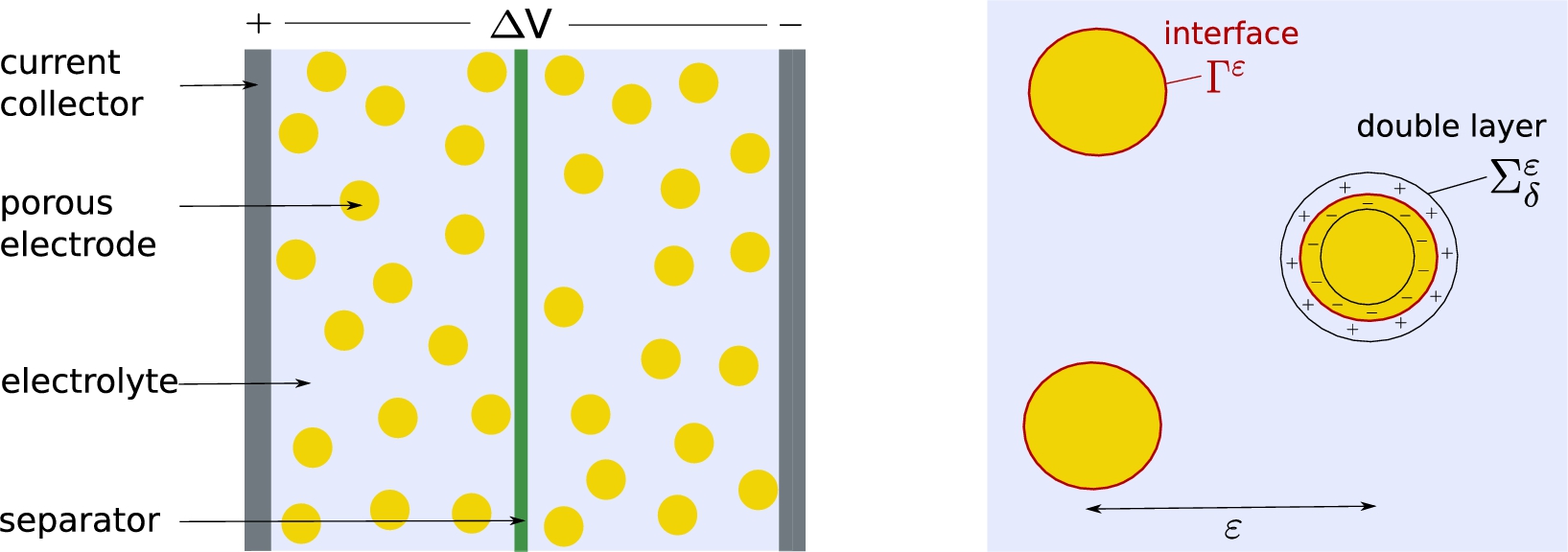
A prospective application of models containing imperfect transmission conditions is the supercapacitor, which is a small electrochemical device to store energy. The high capacity of the device is obtained by maximizing the surface area to volume ratio, which is achieved by taking a porous electrode, see Fig. 2.

Let us study the stationary current flow in such a device. First of all we note that discontinuities of the potential are in principle nonphysical. However, when considering a double-layer4

⁴

The double-layer $Σ_{δ}^{ε} \subset R^{3}$ is given via the δ-neighborhood of the interface $Γ^{ε}$ as sketched in Fig. 2.

Σ_{δ}^{ε}

, where the thickness of the layer δ is much smaller than the pore size ε, we can reduce the double-layer model to an interface model: In [13], the asymptotic limit

δ \to 0

was studied for one single electrode and one obtains that the normal of the electric displacement across the interface

Γ^{ε}

is equal to the surface charge density in one single layer,5

⁵

The surface charge density $Q^{SL} = {lim}_{δ \to 0} \int_{0}^{δ} q_{δ} d x$ is the line integral of the charge density $q_{δ}$ .

i.e.

D \cdot n = Q^{SL}

. Hereby,

D = ϵ_{r} ϵ_{0} E

depends on the relative permittivity

ϵ_{r}

, the vacuum permittivity

ϵ_{0}

, and the electric field E, where

E = - \nabla φ

is given via the electrostatic potential φ. Using a linearization argument, we obtain that

Q^{SL}

is proportional to the difference of the electric potential, i.e.

Q^{SL} = C (φ_{1} - φ_{2})

, where the proportionality factor C denotes the capacity per surface element.6

⁶

The relation between current flux and potential difference is in general not linear, since the capacity depends nonlinearly on the electric potential, see e.g. [23].

Thus, we obtain the interface condition

- ϵ_{r} ϵ_{0} \nabla φ_{1}^{ε} \cdot n_{1}^{ε} = C (ε) (φ_{1}^{ε} - φ_{2}^{ε})

Γ^{ε}

. Realizing that the total capacity of each electrode

C (ε) A \sim A / d

is proportional to the ratio of its surface area A divided by the distance between two electrodes

d \sim ε

yields

C (ε) \sim ε^{- 1}

as in the case (ii). For Carbon-based electrodes, characteristic pore sizes are

2 - 50

nanometers, see e.g. [30], and the macroscopic length scale of the device is about several hundreds micrometers. Hence, the parameter ε is of order

10^{- 5}

–

10^{- 4}

Fig. 2.

The main components of a supercapacitor (left) and the double layer (right).

Footnotes

Acknowledgements

The author thanks C. Guhlke, M. Landstorfer, and D. Peschka for helpful discussions on possible applications in Section . Moreover, the author thanks M. Gahn as well as the anonymous referee for their suggestions, which improved the quality of the text a lot. The research of S.R. was supported by Deutsche Forschungsgesellschaft within Collaborative Research Center 910: Control of self-organizing nonlinear systems: Theoretical methods and concepts of application via the project A5: Pattern formation in systems with multiple scales.

Auxiliary estimates

References

Acerbi,

Chiadò Piat,

Dal Maso and

Percivale, An extension theorem from connected sets, and homogenization in general periodic domains, Nonlinear Anal. 18(5) (1992), 481–496. doi:10.1016/0362-546X(92)90015-7.

Ainouz, Homogenization of a dual-permeability problem in two-component media with imperfect contact, Appl Math. 60(2) (2015), 185–196. doi:10.1007/s10492-015-0090-x.

Canon and

J.N.

Pernin, Homogénéisation d’un problème de diffusion en milieu composite avec barrière à l’interface, C R Acad Sci Paris Sèr I Math. 325(1) (1997), 123–126. doi:10.1016/S0764-4442(97)83946-8.

Cioranescu,

Damlamian,

Donato,

Griso and

Zaki, The periodic unfolding method in domains with holes, SIAM J Math Anal. 44(2) (2012), 718–760. doi:10.1137/100817942.

Cioranescu,

Damlamian and

Griso, The periodic unfolding method in homogenization, SIAM J Math Anal. 40(4) (2008), 1585–1620. doi:10.1137/080713148.

Cioranescu,

Donato and

Zaki, The periodic unfolding method in perforated domains, Port Math (NS) 63(4) (2006), 467–496.

Cioranescu and

J.S.J.

Paulin, Homogenization in open sets with holes, J Math Anal Appl. 71(2) (1979), 590–607. doi:10.1016/0022-247X(79)90211-7.

Donato,

Faella and

Monsurrò, Homogenization of the wave equation in composites with imperfect interface: A memory effect, J Math Pures Appl (9) 87(2) (2007), 119–143. doi:10.1016/j.matpur.2006.11.004.

Donato and

K.H.

Le Nguyen, Homogenization of diffusion problems with a nonlinear interfacial resistance, NoDEA Nonlinear Differential Equations Appl. 22(5) (2015), 1345–1380. doi:10.1007/s00030-015-0325-2.

10.

Donato,

K.H.

Le Nguyen and

Tardieu, The periodic unfolding method for a class of imperfect transmission problems, J Math Sci (NY) 176(6) (2011), 891–927. Problems in mathematical analysis. No. 58. doi:10.1007/s10958-011-0443-2.

11.

Donato and

Monsurrò, Homogenization of two heat conductors with an interfacial contact resistance, Anal Appl (Singap) 2(3) (2004), 247–273. doi:10.1142/S0219530504000345.

12.

Donato and

Ţenţea, Homogenization of an elastic double-porosity medium with imperfect interface via the periodic unfolding method, Bound Value Probl. 2013(265) (2013), 14.

13.

Dreyer,

Guhlke and

Müller, Modeling of electrochemical double layers in thermodynamic non-equilibrium, Phys Chem Chem Phys. 17 (2015), 27176–27194. doi:10.1039/C5CP03836G.

14.

Fatima,

Muntean and

Ptashnyk, Unfolding-based corrector estimates for a reaction-diffusion system predicting concrete corrosion, Appl Anal. 91(6) (2012), 1129–1154. doi:10.1080/00036811.2011.625016.

15.

Griso, Error estimate and unfolding for periodic homogenization, Asymptot Anal. 40(3–4) (2004), 269–286.

16.

Griso, Interior error estimate for periodic homogenization, C R Math Acad Sci Paris. 340(3) (2005), 251–254. doi:10.1016/j.crma.2004.10.027.

17.

Griso, Error estimates in periodic homogenization with a non-homogeneous Dirichlet condition, 2013, arXiv:13084110.

18.

Grisvard, Elliptic Problems in Nonsmooth Domains, Monographs and Studies in Mathematics, Vol. 24, Pitman (Advanced Publishing Program), Boston, MA, 1985.

19.

Hanke, Homogenization in gradient plasticity, Math Models Methods Appl Sci. 21 (2011), 1651–1684. doi:10.1142/S0218202511005520.

20.

Heida, An extension of the stochastic two-scale convergence method and application, Asymptot Anal. 72(1–2) (2011), 1–30.

21.

H.K.

Hummel, Homogenization for heat transfer in polycrystals with interfacial resistances, Appl Anal. 75(3–4) (2000), 403–424. doi:10.1080/00036810008840857.

22.

E.C.

Jose, Homogenization of a parabolic problem with an imperfect interface, Rev Roumaine Math Pures Appl. 54(3) (2009), 189–222.

23.

Landstorfer,

Guhlke and

Dreyer, Theory and structure of the metal-electrolyte interface incorporating adsorption and solvation effects, Electrochimica Acta. 201 (2016), 187–219. doi:10.1016/j.electacta.2016.03.013.

24.

K.H.

Le Nguyen, Homogenization of heat transfer process in composite materials, J Elliptic Parabol Equ. 1 (2015), 175–188. doi:10.1007/BF03377374.

25.

Mielke,

Reichelt and

Thomas, Two-scale homogenization of nonlinear reaction-diffusion systems with slow diffusion, Netw Heterog Media. 9(2) (2014), 353–382. doi:10.3934/nhm.2014.9.353.

26.

Monsurrò, Homogenization of a two-component composite with interfacial thermal barrier, Adv Math Sci Appl. 13(1) (2003), 43–63.

27.

Nečas, Les Méthodes Directes en Théorie des Equations Elliptiques, Masson et Cie, Éditeurs, Paris; Academia, Éditeurs, Prague, 1967.

28.

Reichelt, Error estimates for elliptic equations with not-exactly periodic coefficients, Advances in Mathematical Sciences and Applications. 25(1) (2016), 117–131.

29.

Reichelt, Two-scale homogenization of systems of nonlinear parabolic equations, Humboldt-Universität zu Berlin, 2015, http://edoc.hu-berlin.de/dissertationen/reichelt-sina-2015-11-27/PDF/reichelt.pdf.

30.

Simon and

Gogotsi, Materials for electrochemical capacitors, Nature Materials. 7 (2008), 845–854. doi:10.1038/nmat2297.

Corrector estimates for a class of imperfect transmission problems

Abstract

Keywords

1. Introduction

3. Periodic unfolding

1 Note that L p ( Ω × Y ) and L p ( Ω ; L p ( Y ) ) can be identified for 1 ⩽ p < ∞ , whereas this fails for p = ∞ .

4.1. The case − 1 < γ < 1

Proposition 6.1 ([15, Prop. 4.3]).

7.1. Application to supercapacitors

Footnotes

Acknowledgements

Auxiliary estimates

References

¹
Note that $L^{p} (Ω \times Y)$ and $L^{p} (Ω; L^{p} (Y))$ can be identified for $1 ⩽ p < \infty$ , whereas this fails for $p = \infty$ .

4.1. The case $- 1 < γ < 1$