Fundamental gaps of the Gross–Pitaevskii equation with repulsive interaction

Abstract

We study asymptotically and numerically the fundamental gaps (i.e. the difference between the first excited state and the ground state) in energy and chemical potential of the Gross–Pitaevskii equation (GPE) – nonlinear Schrödinger equation with cubic nonlinearity – with repulsive interaction under different trapping potentials including box potential and harmonic potential. Based on our asymptotic and numerical results, we formulate a gap conjecture on the fundamental gaps in energy and chemical potential of the GPE on bounded domains with the homogeneous Dirichlet boundary condition, and in the whole space with a convex trapping potential growing at least quadratically in the far field. We then extend these results to the GPE on bounded domains with either the homogeneous Neumann boundary condition or periodic boundary condition.

Keywords

Gross–Pitaevskii equation fundamental gap ground state first excited state energy asymptotics repulsive interaction

1. Introduction

The time-independent Schrödinger equation (in dimensionless form by taking $ℏ = m = 1$ with m the mass of the particle) [5,24,27,34] $\begin{matrix} (1.1) & H Φ : = [\sum_{j = 1}^{N} (- \frac{1}{2} Δ_{j} + V (r_{j})) + \sum_{1 ⩽ j < k ⩽ N} V_{int} (r_{j} - r_{k})] Φ = E Φ, \end{matrix}$ has been widely used in quantum physics and chemistry to mathematically predict the property of a quantum system with N particles (usually atoms, molecules, and subatomic particles whether free, bound or localized). Here $r_{j} \in R^{3}$ is the spatial coordinate of the jth particle, $Δ_{j}$ is the Laplacian operator with respect to the spatial coordinate $r_{j}$ for $j = 1, 2, \dots, N$ , $Φ : = Φ (r_{1}, \dots, r_{N})$ is the complex-valued wave function of the quantum system, $V (r)$ (for $r \in R^{3}$ ) is a given real-valued potential, $V_{int} (r)$ is a given real-valued interaction kernel for two-body interaction satisfying $V_{int} (r) = V_{int} (- r)$ and H is the Hamiltonian operator. When the wave function is normalized as $\int_{R^{3 N}} | Φ |^{2} d r_{1} \dots d r_{N} = 1$ , E is the total energy of the quantum system with respect to the wave function Φ. The time-independent Schrödinger equation (1.1), also an eigenvalue problem in mathematics, predicts that wave function can form stationary states including ground and excited states [5,24,27,34]. Finding the ground state and its energy, as well as the energy gap (or band gap) between the ground and first excited states via Eq. (1.1) has become a fundamental and highly challenging problem in computational quantum physics and chemistry, as well as material simulation and design [17 ,18 ,23 ,25 ,30 ,31].

By setting $N = 1$ in Eq. (1.1) and performing a dimension reduction from three dimensions (3D) to two dimensions (2D) and one dimension (1D) under proper assumptions on the potential $V (r)$ such that separation of (the spatial) variables for the wave function is valid [6,7,12,21,32], one can get the d-dimensional ( $d = 3, 2, 1$ ) time-independent Schrödinger equation with complex-valued wave function $ϕ : = ϕ (x)$ , which has been widely used in the physics literature [5,24,27,34] $\begin{matrix} (1.2) & H ϕ : = (- \frac{1}{2} Δ_{x} + V (x)) ϕ (x) = E ϕ (x), x = {(x_{1}, \dots, x_{d})}^{T} \in Ω \subseteq R^{d} . \end{matrix}$ Using the rescaling formulas $y = \sqrt{2} x \in R^{d}$ and $φ (y) = 2^{- d / 4} ϕ (x)$ , one can derive the following time-independent Schrödinger equation [2–4,36] $\begin{matrix} (1.3) & L φ : = [- Δ_{y} + W (y)] φ (y) = E φ (y), y \in U \subseteq R^{d}, \end{matrix}$ where $W (y) = V (x) = V (y / \sqrt{2})$ , $U = {y | y / \sqrt{2} \in Ω}$ and the operator $L : = - Δ_{y} + W (y)$ is called the Schrödinger operator [3]. If U is bounded, then we require the homogeneous Dirichlet boundary condition (BC) $φ (y) |_{\partial U} = 0$ to be imposed. In this case, we can also simply define $W (y) = + \infty$ for y outside U and Eq. (1.3) can be defined in the whole space without BC. If $W (y)$ is bounded below in U, i.e. ${inf}_{y \in U} W (y) > - \infty$ , without loss of generality, we can always assume that $W (y) ⩾ 0$ for $y \in U$ when we are interested in the ground and excited states and the energy gap. Under proper assumptions on the potential $W (y)$ , the eigenvalues $E_{g}, E_{1}, E_{2}, \dots$ of the Sturm–Liouville eigenvalue problem (1.3) under the normalization condition [3] $\begin{matrix} (1.4) & ‖ φ ‖_{2}^{2} : = \int_{U} {| φ (y) |}^{2} d y = 1 ⟺ ‖ ϕ ‖_{2}^{2} : = \int_{Ω} {| ϕ (x) |}^{2} d x = 1, \end{matrix}$ are real and can be ordered such that $0 < E_{g} < E_{1} ⩽ E_{2} ⩽ \dots$ with corresponding eigenfunctions (or stationary states) $φ_{g} (y), φ_{1} (y), φ_{2} (y), \dots$ . Then $φ_{g} (y)$ and $φ_{1} (y)$ are called the ground state and the first excited state, respectively. $δ_{0} : = E_{1} - E_{g} > 0$ is usually called the fundamental gap in the literature [3,4,36]. Assuming that U is a bounded convex domain and the potential $W (y) \in C^{0} (U)$ is a continuous function, based on results for special cases, the gap conjecture was formulated in the literature [3,4,36] as: $\begin{matrix} (1.5) & δ_{0} = E_{1} - E_{g} ⩾ \frac{3 π^{2}}{D_{U}^{2}}, with D_{U} : = sup_{y, z \in U} | y - z | . \end{matrix}$ The gap conjecture is sharp when $d = 1$ , $U = (0, L)$ with $0 < L \in R$ and $W (y) \equiv 0$ for $y \in U$ [3]. Recently, by the use of the gradient flow and geometric analysis and assuming that $W (y) \in C^{0} (U)$ is convex, Andrews and Clutterbuck proved the gap conjecture [2]. In addition, they showed that if $U = R^{d}$ and the potential $W (y)$ satisfies $D^{2} W (y) ⩾ γ_{w}^{2} I_{d}$ for $y \in R^{d}$ with $γ_{w} > 0$ , where $I_{d}$ is the identity matrix in d-dimensions, the fundamental gap described by Eq. (1.3) under the condition (1.4) satisfies $δ_{0} : = E_{1} - E_{g} ⩾ \sqrt{2} γ_{w}$ [2].

In this paper, we will consider the dimensionless time-independent Gross–Pitaevskii equation (GPE) in d-dimensions ( $d = 3, 2, 1$ ) [6,7,12,21,32] $\begin{matrix} (1.6) & [- \frac{1}{2} Δ + V (x) + β {| ϕ (x) |}^{2}] ϕ (x) = μ ϕ (x), x \in Ω \subseteq R^{d}, \end{matrix}$ where $ϕ : = ϕ (x)$ is the complex-valued wave function (or eigenfunction) normalized via (1.4), $V : = V (x)$ is a given real-valued potential, $β ⩾ 0$ is a dimensionless constant describing the repulsive (defocussing) interaction strength, and the eigenvalue (or chemical potential in the physics literature) $μ : = μ (ϕ)$ is defined as [6,7,21,32] $\begin{matrix} (1.7) & μ (ϕ) = E (ϕ) + \frac{β}{2} \int_{Ω} {| ϕ (x) |}^{4} d x, \end{matrix}$ with the energy $E : = E (ϕ)$ defined as [7] $\begin{matrix} (1.8) & E (ϕ) = \int_{Ω} [\frac{1}{2} {| \nabla ϕ (x) |}^{2} + V (x) {| ϕ (x) |}^{2} + \frac{β}{2} {| ϕ (x) |}^{4}] d x . \end{matrix}$ Again, if Ω is bounded, the homogeneous Dirichlet BC, i.e. $ϕ (x) |_{\partial Ω} = 0$ , needs to be imposed. Thus, the time-independent GPE (1.6) is a nonlinear eigenvalue problem under the constraint (1.4). It is a mean field model arising from Bose–Einstein condensates (BECs) [1,6,21,26] that can be obtained from the Schrödinger equation (1.1) via the Hartree ansatz and mean field approximation [7,20,28,32]. When $β = 0$ , it collapses to the time-independent Schrödinger equation (1.2). It is worth mentioning that if the domain U in (1.3) is bounded, the domain Ω in (1.2) (or (1.6)) can be defined as $Ω = {x | \sqrt{2} x \in U}$ via the re-scaling $y = \sqrt{2} x$ . Thus the diameter for the domain Ω becomes $D : = D_{Ω} = D_{U} / \sqrt{2}$ , and the lower bound in the fundamental gap (1.5) for the Schrödinger equation (1.2) becomes $\frac{3 π^{2}}{D_{U}^{2}} = \frac{3 π^{2}}{2 D^{2}}$ .

The ground state of the GPE (1.6) is usually defined as the minimizer of the non-convex minimization problem (or constrained minimization problem) [6,7,21,26] $\begin{matrix} (1.9) & ϕ_{g} = \underset{ϕ \in S}{\arg \min} E (ϕ), \end{matrix}$ where $S = {ϕ | ‖ ϕ ‖_{2}^{2} : = \int_{Ω} | ϕ (x) |^{2} d x = 1, E (ϕ) < \infty, ϕ |_{\partial Ω} = 0 if Ω is bounded}$ . The ground state can be chosen as nonnegative $| ϕ_{g} |$ , i.e. $ϕ_{g} = | ϕ_{g} | e^{i θ}$ for some constant $θ \in R$ and $i = \sqrt{- 1}$ . Moreover, the nonnegative ground state $| ϕ_{g} |$ is unique [7,29]. Thus, from now on, we refer to the ground state as the nonnegative one. It is easy to see that the ground state $ϕ_{g}$ satisfies the time-independent GPE (1.6) and the constraint (1.4). Hence it is an eigenfunction (or stationary state) of (1.6) with the least energy. Any other eigenfunctions of the GPE (1.6) under the constraint (1.4) whose energies are larger than that of the ground state are usually called the excited states in the physics literature [7,21,32]. Specifically, the excited state with the least energy among all excited states is usually called the first excited state, which is denoted as $ϕ_{1}$ .

For the GPE (1.6), the ground state has been obtained asymptotically in weakly and strongly repulsive interaction regimes, i.e. $0 < β ≪ 1$ and $β ≫ 1$ , respectively, for several different trapping potentials [14]. In fact, by ordering all the eigenfunctions of the GPE with a repulsive interaction and a confinement potential, i.e. $β ⩾ 0$ and ${lim}_{| x | \to + \infty} V (x) = + \infty$ , under the constraint (1.4) according to their energies with $ϕ_{g}^{β}, ϕ_{1}^{β}, ϕ_{2}^{β}, \dots$ satisfying $E_{g} (β) : = E (ϕ_{g}^{β}) < E_{1} (β) : = E (ϕ_{1}^{β}) ⩽ E (ϕ_{2}^{β}) ⩽ \dots$ , it can be shown that $μ_{g} (β) : = μ (ϕ_{g}^{β}) < μ_{1} (β) : = μ (ϕ_{1}^{β})$ [19], and thus $ϕ_{1}^{β}$ is usually called the first excited state. We define the fundamental gaps in energy and chemical potential of the time-independent GPE under the constraint (1.4) as $\begin{matrix} (1.10) & \begin{matrix} δ_{E} (β) : = E (ϕ_{1}^{β}) - E (ϕ_{g}^{β}) > 0, δ_{μ} (β) : = μ (ϕ_{1}^{β}) - μ (ϕ_{g}^{β}) > 0, β ⩾ 0, \\ δ_{E}^{\infty} : = inf_{β ⩾ 0} δ_{E} (β), δ_{μ}^{\infty} : = inf_{β ⩾ 0} δ_{μ} (β) . \end{matrix} \end{matrix}$ In general, the first excited state $ϕ_{1}^{β}$ is not unique. Since we are mainly interested in its energy and chemical potential as well as the fundamental gaps, it does not matter which first excited state is taken in our analysis and simulation below. The main purpose of this paper is to study asymptotically and numerically the fundamental gaps of the GPE with different trapping potentials and to formulate a gap conjecture for the GPE. Define the eigenspace of (1.2) corresponding to the eigenvalue $E_{1}$ (the second smallest eigenvalue) as $\begin{matrix} (1.11) & W_{1} = {ϕ (x) : Ω \to C | H ϕ = E_{1} ϕ, ϕ |_{\partial Ω} = 0 if Ω is bounded} . \end{matrix}$ Based on our asymptotic results and extensive numerical results, we propose the following:

Gap Conjecture I (For GPE on bounded domain with homogeneous Dirichlet boundary conditions).

Suppose Ω is a convex bounded domain and the external potential $V (x)$ is convex.

In the non-degenerate case, i.e. when $dim (W_{1}) = 1$ , we have $\begin{matrix} (1.12) & δ_{E}^{\infty} : = inf_{β ⩾ 0} δ_{E} (β) ⩾ \frac{3 π^{2}}{2 D^{2}}, δ_{μ}^{\infty} : = inf_{β ⩾ 0} δ_{μ} (β) ⩾ \frac{3 π^{2}}{2 D^{2}} . \end{matrix}$

In the degenerate case, i.e. when $dim (W_{1}) ⩾ 2$ , we have $\begin{matrix} (1.13) & δ_{E}^{\infty} : = inf_{β ⩾ 0} δ_{E} (β) ⩾ \frac{π^{2}}{2 D^{2}}, δ_{μ}^{\infty} : = inf_{β ⩾ 0} δ_{μ} (β) ⩾ \frac{3 π^{2}}{8 D^{2}} . \end{matrix}$

The rest of this paper is organized as follows. In Section 2, we study asymptotically and numerically the fundamental gaps of GPE on bounded domains with homogeneous Dirichlet BC to show the gap conjectures (1.12) and (1.13). In Section 3, we obtain results for GPE in the whole space with a confinement potential. Extension to GPE on bounded domains with either periodic or homogeneous Neumann BC are presented in Section 4. Finally, some conclusions are drawn in Section 5. For simplicity of notations, denote $Ω_{0} = \prod_{j = 1}^{d} (0, L_{j})$ satisfying $L_{1} ⩾ L_{2} ⩾ \dots ⩾ L_{d} > 0$ and $A_{0} = 1 / \sqrt{\prod_{j = 1}^{d} L_{j}}$ .

2. On bounded domains with homogeneous Dirichlet BC

In this section, we obtain fundamental gaps of the GPE (1.6) on a bounded domain Ω with homogeneous Dirichlet BC asymptotically under a box potential and numerically under a general potential. Based on the results, we formulate a novel gap conjecture. The bounded domain problem with homogeneous Dirichlet boundary conditions can also be viewed as a whole space problem by letting $V (x) = \infty$ for $x \in Ω^{c}$ .

2.1. Non-degenerate case, i.e. $dim (W_{1}) = 1$

We first consider a special case by taking $Ω = Ω_{0}$ satisfying $d = 1$ or $L_{1} > L_{2}$ when $d ⩾ 2$ and $V (x) \equiv 0$ for $x \in Ω$ in (1.6). For simplicity, we define $\begin{matrix} (2.1) & A_{1} = \frac{2}{L_{1}} (\frac{25}{9 L_{1}} + \frac{2}{9} \sum_{j = 1}^{d} \frac{1}{L_{j}}), A_{2} = \frac{π^{2}}{2} \sum_{j = 1}^{d} \frac{1}{L_{j}^{2}} . \end{matrix}$

In this scenario, when $β = 0$ , all the eigenfunctions can be obtained via the sine series [13,14]. Thus the ground state $ϕ_{g}^{0} (x)$ and the first excited state $ϕ_{1}^{0} (x)$ can be given explicitly as [13,14] for $x \in \bar{Ω}$ $\begin{matrix} (2.2) & ϕ_{g}^{0} (x) = 2^{\frac{d}{2}} A_{0} \prod_{j = 1}^{d} sin (\frac{π x_{j}}{L_{j}}), ϕ_{1}^{0} (x) = 2^{\frac{d}{2}} A_{0} sin (\frac{2 π x_{1}}{L_{1}}) \prod_{j = 2}^{d} sin (\frac{π x_{j}}{L_{j}}) . \end{matrix}$

Lemma 2.1.
In the weakly repulsive interaction regime, i.e. $0 < β ≪ 1$ , we have $\begin{array}{l} (2.3) & E_{g} (β) & = A_{2} + \frac{3^{d} A_{0}^{2}}{2^{d + 1}} β + o (β), μ_{g} (β) = A_{2} + \frac{3^{d} A_{0}^{2}}{2^{d}} β + o (β), \\ (2.4) & E_{1} (β) & = \frac{3 π^{2}}{2 L_{1}^{2}} + A_{2} + \frac{3^{d} A_{0}^{2}}{2^{d + 1}} β + o (β), μ_{1} (β) = \frac{3 π^{2}}{2 L_{1}^{2}} + A_{2} + \frac{3^{d} A_{0}^{2}}{2^{d}} β + o (β) . \end{array}$
Proof.
When $0 < β ≪ 1$ , we can approximate the ground state $ϕ_{g}^{β} (x)$ and the first excited state $ϕ_{1}^{β} (x)$ by $ϕ_{g}^{0} (x)$ and $ϕ_{1}^{0} (x)$ , respectively. Thus we have $\begin{matrix} (2.5) & ϕ_{g}^{β} (x) \approx ϕ_{g}^{0} (x), ϕ_{1}^{β} (x) \approx ϕ_{1}^{0} (x), x \in \bar{Ω} . \end{matrix}$ Plugging (2.5) into (1.7) and (1.8), after a detailed computation which is omitted here for brevity, we can obtain (2.3)–(2.4). □

Lemma 2.1 implies that $δ_{E} (β) = E_{1} (β) - E_{g} (β) \approx \frac{3 π^{2}}{2 L_{1}^{2}}$ and $δ_{μ} (β) = μ_{1} (β) - μ_{g} (β) \approx \frac{3 π^{2}}{2 L_{1}^{2}}$ for $0 < β ≪ 1$ , which are independent of β. In order to get the dependence on β, we need to find more accurate approximations of $ϕ_{g}^{β}$ and $ϕ_{1}^{β}$ and can obtain the following asymptotics of the fundamental gaps.
Lemma 2.2.
When $0 ⩽ β ≪ 1$ , we have $\begin{matrix} (2.6) & δ_{E} (β) = \frac{3 π^{2}}{2 L_{1}^{2}} + G_{d}^{(1)} β^{2} + o (β^{2}), δ_{μ} (β) = \frac{3 π^{2}}{2 L_{1}^{2}} + G_{d}^{(2)} β^{2} + o (β^{2}), \end{matrix}$ where $\begin{matrix} G_{d}^{(1)} = \{\begin{matrix} \frac{3}{64 π^{2}}, \\ \frac{A_{0}^{4}}{64 π^{2}} (\frac{27}{4} L_{1}^{2} + \frac{3}{A_{6} (A_{6} L_{1}^{2} + 3)}), \\ \frac{1}{256 π^{2}} (C_{1, 1, 1} - C_{2, 1, 1}), \end{matrix} G_{d}^{(2)} = \{\begin{matrix} \frac{9}{64 π^{2}}, & d = 1, \\ \frac{3 A_{0}^{4}}{64 π^{2}} (\frac{27}{4} L_{1}^{2} + \frac{3}{A_{6} (A_{6} L_{1}^{2} + 3)}), & d = 2, \\ \frac{3}{256 π^{2}} (C_{1, 1, 1} - C_{2, 1, 1}), & d = 3, \end{matrix} \end{matrix}$ with $\begin{matrix} (2.7) & A_{6} = \sum_{j = 1}^{d} \frac{1}{L_{j}^{2}}, C_{k_{1}, k_{2}, k_{3}} = A_{0}^{4} (81 \sum_{j = 1}^{3} \frac{L_{j}^{2}}{k_{j}^{2}} + 9 \sum_{i < j} \frac{1}{\frac{k_{i}^{2}}{L_{i}^{2}} + \frac{k_{j}^{2}}{L_{j}^{2}}} + \frac{1}{\sum_{j = 1}^{3} \frac{k_{j}^{2}}{L_{j}^{2}}}) . \end{matrix}$
Proof.
When $0 < β ≪ 1$ , we assume $\begin{matrix} (2.8) & ϕ_{g}^{β} (x) \approx ϕ_{g}^{0} (x) + β φ_{g} (x) + o (β), x \in Ω . \end{matrix}$ Plugging (2.8) into (1.6), noticing (2.2), (2.3) and (2.4), and dropping all terms at $O (β^{2})$ and above, we obtain $\begin{matrix} (2.9) & Δ φ_{g} (x) + 2 A_{2} φ_{g} (x) = 2 {(ϕ_{g}^{0} (x))}^{3} - \frac{3^{d} A_{0}^{2}}{2^{d - 1}} ϕ_{g}^{0} (x), x \in Ω, φ_{g} (x) |_{\partial Ω} = 0 . \end{matrix}$ Substituting (2.2) into (2.9), we can solve it analytically. For the simplicity of notations, here we only present the case when $d = 1$ . Extensions to $d = 2$ and $d = 3$ are straightforward and the details are omitted here for brevity [33]. When $d = 1$ , we have $\begin{matrix} (2.10) & φ_{g} (x) = \frac{\sqrt{2 L_{1}}}{8 π^{2}} sin (\frac{3 π x}{L_{1}}), 0 ⩽ x ⩽ L_{1} . \end{matrix}$ Plugging (2.10) into (2.8) and using $‖ ϕ_{g}^{β} ‖_{2} = 1$ , we get $\begin{matrix} (2.11) & ϕ_{g}^{β} (x) \approx \sqrt{\frac{64 π^{4} - β^{2} L_{1}^{2}}{32 π^{4} L_{1}}} sin (\frac{π x}{L_{1}}) + \frac{β \sqrt{2 L_{1}}}{8 π^{2}} sin (\frac{3 π x}{L_{1}}), 0 ⩽ x ⩽ L_{1} . \end{matrix}$ Inserting (2.11) into (1.8) and (1.7) with $V (x) \equiv 0$ , we have $\begin{matrix} (2.12) & E_{g} (β) = \frac{π^{2}}{2 L_{1}^{2}} + \frac{3 β}{4 L_{1}} - \frac{β^{2}}{16 π^{2}} + o (β^{2}), μ_{g} (β) = \frac{π^{2}}{2 L_{1}^{2}} + \frac{3 β}{2 L_{1}} - \frac{3 β^{2}}{16 π^{2}} + o (β^{2}) . \end{matrix}$ Similarly, we can obtain results for the first excited state $\begin{matrix} (2.13) & E_{1} (β) = \frac{2 π^{2}}{L_{1}^{2}} + \frac{3 β}{4 L_{1}} - \frac{β^{2}}{64 π^{2}} + o (β^{2}), μ_{1} (β) = \frac{2 π^{2}}{L_{1}^{2}} + \frac{3 β}{2 L_{1}} - \frac{3 β^{2}}{64 π^{2}} + o (β^{2}) . \end{matrix}$ Subtracting (2.12) from (2.13), we obtain (2.6) when $d = 1$ . □
Lemma 2.3.
In the strongly repulsive interaction regime, i.e. $β ≫ 1$ , we have $\begin{array}{l} (2.14) & E_{g} (β) = \frac{A_{0}^{2}}{2} β + \frac{4 A_{0} A_{3}}{3} β^{\frac{1}{2}} + 2 A_{3}^{2} - \frac{8 A_{4}}{9} + o (1), \\ (2.15) & μ_{g} (β) = A_{0}^{2} β + 2 A_{0} A_{3} β^{\frac{1}{2}} + 2 A_{3}^{2} - A_{4} + o (1), β ≫ 1, \\ (2.16) & E_{1} (β) = \frac{A_{0}^{2}}{2} β + \frac{4 A_{0} (A_{3} L_{1} + 1)}{3 L_{1}} β^{\frac{1}{2}} + \frac{2 {(A_{3} L_{1} + 1)}^{2}}{L_{1}^{2}} - \frac{8 A_{5}}{9} + o (1), \\ (2.17) & μ_{1} (β) = A_{0}^{2} β + \frac{2 A_{0} (A_{3} L_{1} + 1)}{L_{1}} β^{\frac{1}{2}} + \frac{2 {(A_{3} L_{1} + 1)}^{2}}{L_{1}^{2}} - A_{5} + o (1), \end{array}$ where $\begin{matrix} (2.18) & A_{3} = \sum_{j = 1}^{d} \frac{1}{L_{j}}, A_{4} = 4 \sum_{1 ⩽ j < k ⩽ d} \frac{1_{{d ⩾ 2}}}{L_{j} L_{k}}, A_{5} = A_{4} + 4 \sum_{1 < j ⩽ d} \frac{1_{{d ⩾ 2}}}{L_{1} L_{j}}, \end{matrix}$ with $1_{{d ⩾ 2}}$ the standard set function, which takes 1 when $d ⩾ 2$ and 0 otherwise.
Proof.
When $β ≫ 1$ , the ground and first excited states can be approximated by the Thomas–Fermi (TF) approximations and/or uniformly accurate matched approximations. For $d = 1$ and $Ω = (0, L)$ , these approximations have been given explicitly and verified numerically in the literature [10,11,13,14] as $\begin{matrix} (2.19) & ϕ_{g} (x) \approx \sqrt{\frac{μ_{g}}{β}} ϕ_{L, μ_{g}}^{(1)} (x), ϕ_{1} (x) \approx \sqrt{\frac{μ_{1}}{β}} ϕ_{L, μ_{1}}^{(2)} (x), 0 ⩽ x ⩽ L, \end{matrix}$ where $\begin{matrix} (2.20) & \begin{matrix} ϕ_{L, μ}^{(1)} (x) = tanh (\sqrt{μ} x) + tanh (\sqrt{μ} (L - x)) - tanh (\sqrt{μ} L), 0 ⩽ x ⩽ L, \\ ϕ_{L, μ}^{(2)} (x) = tanh (\sqrt{μ} x) - tanh (\sqrt{μ} (L - x)) + tanh (\sqrt{μ} (L / 2 - x)), \end{matrix} \end{matrix}$ with $μ_{g}$ and $μ_{1}$ determined from the normalization condition (1.4) and $tanh (\sqrt{μ} L) \approx 1$ . These results in 1D can be extended to d-dimensions ( $d = 1, 2, 3$ ) for the approximations of the ground and first excited states as $\begin{array}{l} (2.21) & ϕ_{g}^{β} (x) \approx ϕ_{g}^{MA} (x) = \sqrt{\frac{μ_{g} (β)}{β}} \prod_{j = 1}^{d} ϕ_{L_{j}, μ_{g}}^{(1)} (x_{j}), x \in \bar{Ω}, \\ (2.22) & ϕ_{1}^{β} (x) \approx ϕ_{1}^{MA} (x) = \sqrt{\frac{μ_{1} (β)}{β}} ϕ_{L_{1}, μ_{1}}^{(2)} (x_{1}) \prod_{j = 2}^{d} ϕ_{L_{j}, μ_{1}}^{(1)} (x_{j}), \end{array}$ where $μ_{g} (β)$ and $μ_{1} (β)$ are determined from the normalization condition (1.4). Inserting (2.21) and (2.22) into (1.7) and (1.8), after a detailed computation which is omitted here for brevity, we can obtain (2.14)–(2.17). □

From Lemmas 2.1–2.3, we have asymptotic results for the fundamental gaps.
Proposition 2.1 (For GPE under a box potential in non-degenerate case).

When $Ω = Ω_{0}$ satisfying $d = 1$ or $L_{1} > L_{2}$ when $d ⩾ 2$ and $V (x) \equiv 0$ for $x \in Ω$ in ( 1.6 ), i.e. GPE with a box potential, we have $\begin{matrix} (2.23) & \begin{matrix} δ_{E} (β) = \{\begin{matrix} \frac{3 π^{2}}{2 L_{1}^{2}} + o (β), \\ \frac{4 A_{0}}{3 L_{1}} β^{\frac{1}{2}} + A_{1} + o (1), \end{matrix} \\ δ_{μ} (β) = \{\begin{matrix} \frac{3 π^{2}}{2 L_{1}^{2}} + o (β), & 0 ⩽ β ≪ 1, \\ \frac{2 A_{0}}{L_{1}} β^{\frac{1}{2}} + \frac{6}{L_{1}^{2}} + o (1), & β ≫ 1 . \end{matrix} \end{matrix} \end{matrix}$

Proof.
When $0 ⩽ β ≪ 1$ , subtracting (2.3) from (2.4), noting (1.10), we obtain (2.23) in this parameter regime. Similarly, when $β ≫ 1$ , subtracting (2.14) and (2.15) from (2.16) and (2.17), respectively, we get (2.23) in this parameter regime. □

Fig. 1.
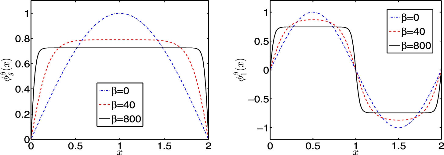
Ground states $ϕ_{g}^{β} (x)$ (left) and first excited states $ϕ_{1}^{β} (x)$ (right) of GPE in 1D with $Ω = (0, 2)$ and a box potential for different $β ⩾ 0$ .

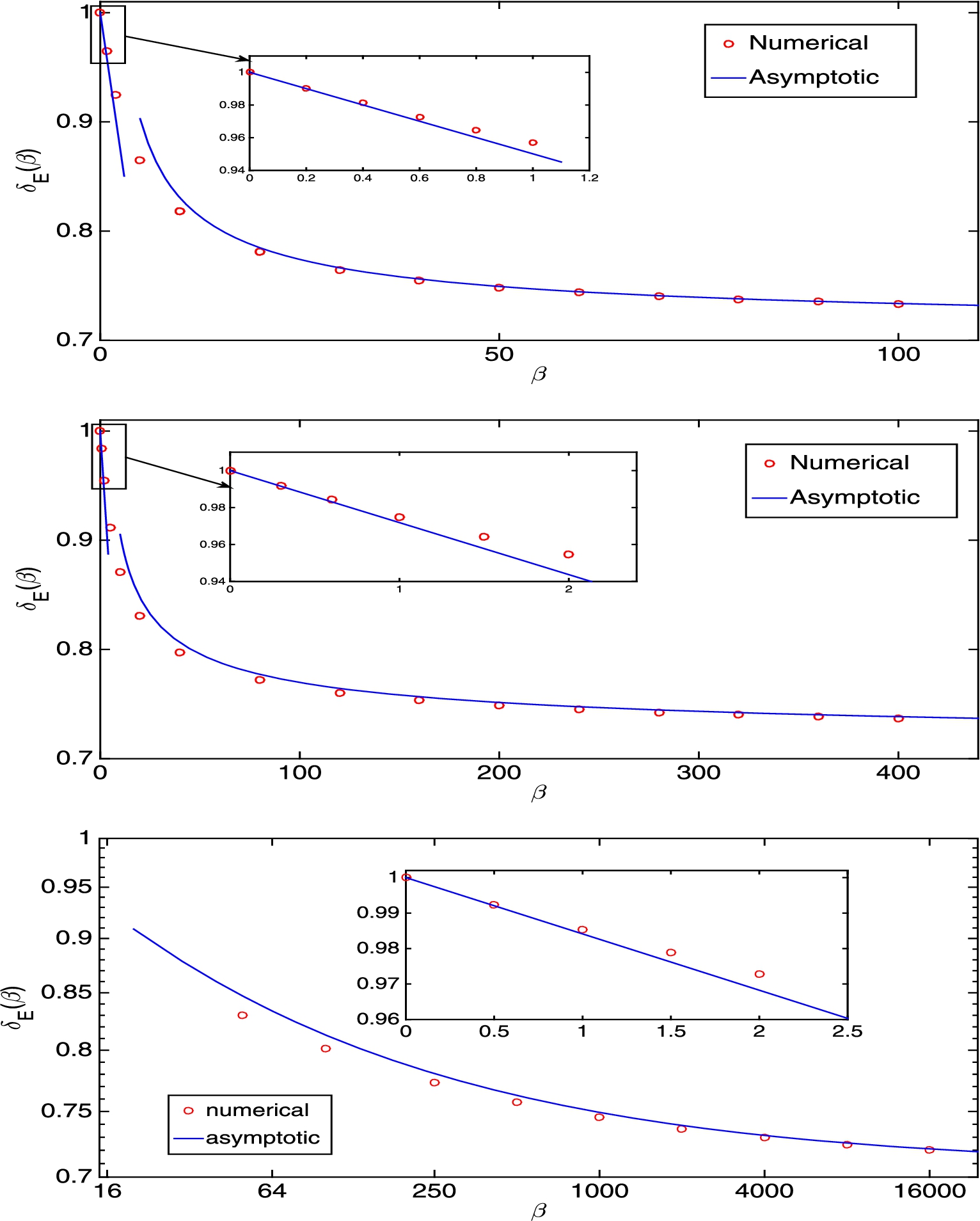
To verify numerically our asymptotic results in Proposition 2.1, we solve the time-independent GPE (1.6) numerically by using the normalized gradient flow via backward Euler finite difference discretization [7–10] to find the ground and first excited states and their corresponding energy and chemical potentials. Figure 1 shows the ground and first excited states for different $β ⩾ 0$ in 1D, Figure 2 shows the energy of the ground and excited states which are excited in $x_{1}$ - or $x_{2}$ -direction, while the first excited state is taken as the one excited in $x_{1}$ -direction, and Fig. 3 depicts fundamental gaps in energy obtained numerically and asymptotically in 1D, 2D and 3D. From Fig. 3, we can see that the asymptotic results in Proposition 2.1 are very accurate in both weakly and strongly repulsive interaction regimes. In addition, our numerical results suggest that both $δ_{E} (β)$ and $δ_{μ} (β)$ are increasing functions for $β ⩾ 0$ (cf. Fig. 3).

Fig. 2.
Energy $E_{g} (β) : = E (ϕ_{g}^{β}) < E_{1} (β) : = E (ϕ_{1}^{β} = ϕ_{1, x_{1}}^{β}) < E_{2} (β) : = E (ϕ_{1, x_{2}}^{β})$ of GPE in 2D with $Ω = (0, 2) \times (0, 1)$ and a box potential for different $β ⩾ 0$ .

Fig. 3.
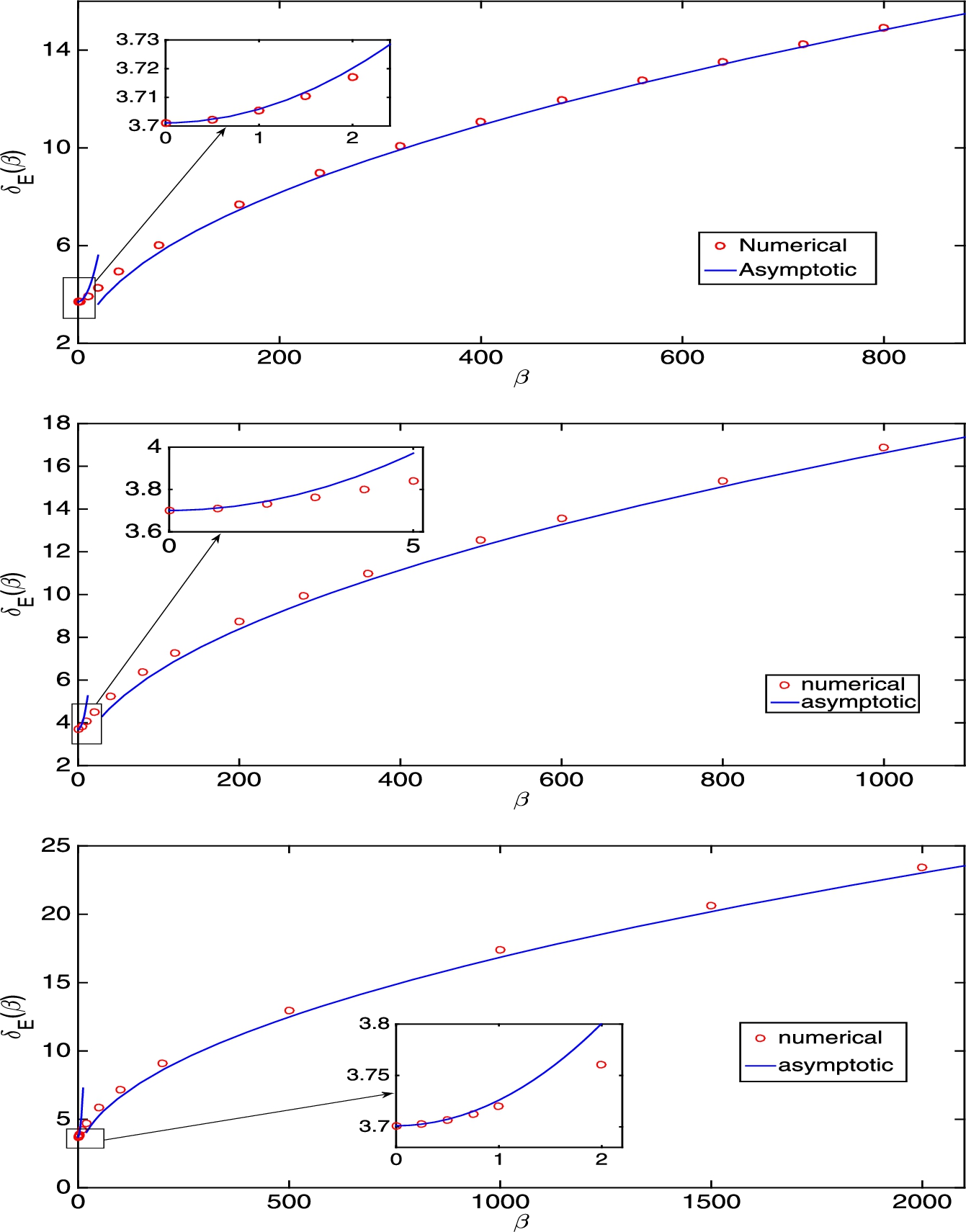
Fundamental gaps in energy of GPE with a box potential in 1D with $Ω = (0, 2)$ (top), in 2D with $Ω = (0, 2) \times (0, 1)$ (middle), and in 3D with $Ω = (0, 2) \times (0, 1) \times (0, 1)$ (bottom).

Fig. 4.
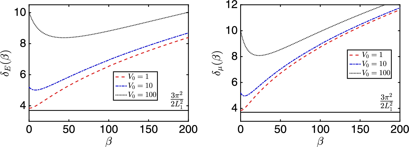
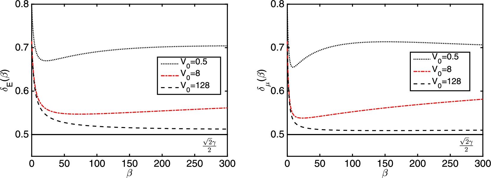
Fundamental gaps in energy $δ_{E} (β)$ (left) and chemical potential $δ_{μ} (β)$ (right) of GPE in 1D with $Ω = (0, 2)$ and $V (x) = V_{0} {(x - 1)}^{2}$ for different $V_{0} > 0$ and $β ⩾ 0$ .

For a general bounded domain Ω and/or $V (x) \neq 0$ , we cannot get asymptotic results on the fundamental gaps, but we can study the problem numerically. If $Ω = Ω_{0}$ and $V (x)$ is symmetric with respect to the axis, we can compute numerically the ground and first excited states and their corresponding energy and chemical potential as well as the fundamental gaps via the Backward Euler finite difference method [7–10]. For arbitrarily chosen external potentials defined in $Ω_{0}$ , the ground state and the first excited state might not have any symmetric property. In this case, we can obtain numerically the ground state and the first excited state by using the numerical method proposed in [15] with spectral discretization in space. Figure 4 depicts fundamental gaps in energy and chemical potential of the GPE in 1D with $Ω = (0, 2)$ and the potential $V (x) = V_{0} {(x - 1)}^{2}$ for different $V_{0}$ and β. Figure 5 plots the fundamental gaps in energy and chemical potential of the GPE in 1D with $Ω = (0, 2)$ and some nonconvex trapping potentials for different $β ⩾ 0$ .

Fig. 5.
Fundamental gaps in energy (left) and chemical potential (right) of GPE in 1D with $Ω = (0, 2)$ and non-convex trapping potentials: (I) $V (x) = - 10 x^{2}$ , and (II) $V (x) = 10 sin (10 (x - 1))$ for different $β ⩾ 0$ .

Based on the asymptotic results in Proposition 2.1 and the above numerical results as well as additional extensive numerical results not shown here for brevity [33], we speculate the gap conjecture (1.12). In fact, our numerical results suggest a stronger gap as $\begin{matrix} (2.24) & \begin{matrix} δ_{E} (β) ⩾ \{\begin{matrix} \frac{3 π^{2}}{2 D^{2}}, & 0 ⩽ β ⩽ \frac{81 π^{4} | Ω |}{64 D^{2}}, \\ \frac{4 β^{1 / 2}}{3 D | Ω |^{1 / 2}}, & β ⩾ \frac{81 π^{4} | Ω |}{64 D^{2}}, \end{matrix} \\ δ_{μ} (β) ⩾ \{\begin{matrix} \frac{3 π^{2}}{2 D^{2}}, & 0 ⩽ β ⩽ \frac{9 π^{4} | Ω |}{16 D^{2}}, \\ \frac{2 β^{1 / 2}}{D | Ω |^{1 / 2}}, & β ⩾ \frac{9 π^{4} | Ω |}{16 D^{2}}, \end{matrix} \end{matrix} \end{matrix}$ where $| Ω |$ is the volume of Ω. On the other hand, Fig. 5 suggests that the gap conjecture (1.12) is not valid for non-convex trapping potentials.
2.2. Degenerate case, i.e. $dim (W_{1}) ⩾ 2$

Again, we first consider a special case by taking $Ω = Ω_{0}$ satisfying $L_{1} = L_{2} : = L$ and $d ⩾ 2$ and $V (x) \equiv 0$ for $x \in Ω$ in (1.6). In this case, the approximations of the ground states and their energy and chemical potential are the same as those in the previous subsection by letting $L_{2} \to L_{1} = L$ . On the contrary, the approximations of the first excited states are completely different with those in the non-degenerate case.

Lemma 2.4.
For weakly repulsive interaction, i.e. $0 < β ≪ 1$ , we have for $d ⩾ 2$ $\begin{array}{l} (2.25) & E_{1} (β) & = \frac{3 π^{2}}{2 L^{2}} + A_{2} + \frac{13 d}{32} A_{0}^{2} β + o (β), μ_{1} (β) = \frac{3 π^{2}}{2 L^{2}} + A_{2} + \frac{13 d}{16} A_{0}^{2} β + o (β) . \end{array}$
Proof.
For simplicity, we only present the 2D case and extension to 3D is straightforward. Denote $\begin{matrix} (2.26) & ϕ_{g}^{0} (x) = \sqrt{\frac{2}{L}} sin (\frac{π x}{L}), ϕ_{1}^{0} (x) = \sqrt{\frac{2}{L}} sin (\frac{2 π x}{L}), 0 ⩽ x ⩽ L . \end{matrix}$ When $d = 2$ and $β = 0$ , it is easy to see that $φ_{1} (x) : = ϕ_{1}^{0} (x_{1}) ϕ_{g}^{0} (x_{2})$ and $φ_{2} (x) : = ϕ_{g}^{0} (x_{1}) ϕ_{1}^{0} (x_{2})$ are two linearly independent orthonormal first excited states. In fact, $W_{1} = span {φ_{1}, φ_{2}}$ . In order to find an appropriate approximation of the first excited state when $0 < β ≪ 1$ , we take an ansatz $\begin{matrix} (2.27) & φ_{a, b} (x) = a φ_{1} (x) + b φ_{2} (x), x = (x_{1}, x_{2}) \in \bar{Ω}, \end{matrix}$ where $a, b \in C$ satisfying $| a |^{2} + | b |^{2} = 1$ implies $‖ φ_{a, b} ‖_{2} = 1$ . Then a and b will be determined by minimizing $E (φ_{a, b})$ . Plugging (2.27) into (1.8), a simple direct computation implies that $\begin{array}{rcl} E (φ_{a, b}) & = & \frac{3 π^{2}}{2 L^{2}} + A_{2} + \frac{8 β}{L^{4}} \iint_{{[0, L]}^{2}} {| a sin (\frac{2 π x_{1}}{L}) sin (\frac{π x_{2}}{L}) + b sin (\frac{π x_{1}}{L}) sin (\frac{2 π x_{2}}{L}) |}^{4} d x \\ = & \frac{3 π^{2}}{2 L^{2}} + A_{2} + \frac{9 β}{8 L^{2}} (| a |^{4} + | b |^{4}) + \frac{β}{2 L^{2}} (4 | a |^{2} | b |^{2} + a^{2} {\bar{b}}^{2} + {\bar{a}}^{2} b^{2}) \\ = & \frac{3 π^{2}}{2 L^{2}} + A_{2} + \frac{9 β}{8 L^{2}} + \frac{β}{4 L^{2}} (2 a^{2} {\bar{b}}^{2} + 2 {\bar{a}}^{2} b^{2} - | a |^{2} | b |^{2}) . \end{array}$ To minimize $E (φ_{a, b})$ , noting $| a |^{2} + | b |^{2} = 1$ , we take $a = e^{i ξ} cos (θ)$ and $b = e^{i η} sin (θ)$ with $ξ, η, θ \in [- π, π)$ . Then we have $\begin{matrix} E (φ_{a, b}) = \frac{3 π^{2}}{2 L^{2}} + A_{2} + \frac{9 β}{8 L^{2}} - \frac{β}{16 L^{2}} {sin}^{2} (2 θ) [1 - 4 cos (2 (ξ - η))], \end{matrix}$ which is minimized when $θ = \pm π / 4$ and $ξ - η = \pm π / 2$ , i.e. $a = \pm i b$ . By taking $a = 1 / \sqrt{2}$ and $b = i / \sqrt{2}$ , we obtain an approximation of the first excited state $ϕ_{1}^{β}$ when $0 < β ≪ 1$ as $\begin{matrix} (2.28) & ϕ_{1}^{β} (x) \approx \frac{1}{\sqrt{2}} [ϕ_{1}^{0} (x_{1}) ϕ_{g}^{0} (x_{2}) + i ϕ_{g}^{0} (x_{1}) ϕ_{1}^{0} (x_{2})], x \in \bar{Ω} . \end{matrix}$ Substituting (2.28) into (1.8) and (1.7), we get (2.25) when $d = 2$ . □
Lemma 2.5.
When $d = 2$ and $β ≫ 1$ , we have $\begin{array}{l} (2.29) & E_{1} (β) = \frac{β}{2 L^{2}} + \frac{8 \sqrt{β}}{3 L^{2}} + \frac{π}{2 L^{2}} ln (β) + o (ln (β)), \\ (2.30) & μ_{1} (β) = \frac{β}{L^{2}} + \frac{4 \sqrt{β}}{L^{2}} + \frac{π}{2 L^{2}} ln (β) + o (ln (β)) . \end{array}$
Proof.
From Lemma 2.4, when $0 < β ≪ 1$ , the first excited state needs to be taken as a vortex-type solution. By assuming that there is no band crossing when $β > 0$ , then the first excited state can be well approximated by the vortex-type solution when $β ≫ 1$ too. Thus when $β ≫ 1$ , we approximate the first excited state via a matched asymptotic approximation.
In the outer region, i.e. $| x - (L / 2, L / 2) | > o (1)$ , it is approximated by the ground state profile as $\begin{matrix} (2.31) & ϕ_{1}^{β} (x) \approx ϕ^{out} (x) = \sqrt{\frac{μ_{1}}{β}} ϕ_{L, μ_{1}}^{(1)} (x_{1}) ϕ_{L, μ_{1}}^{(1)} (x_{2}), \end{matrix}$ where $ϕ_{L, μ}^{(1)} (x)$ is given in (2.20) with $μ = μ_{1} (β)$ the chemical potential of the first excited state.

In the inner region near the center $(L / 2, L / 2)$ , i.e. $| x - (L / 2, L / 2) | ≪ 1$ , it is approximated by a vortex solution with winding number $m = 1$ as $\begin{matrix} (2.32) & ϕ_{1}^{β} (x) \approx ϕ^{in} (x) = \sqrt{\frac{μ_{1}}{β}} f (r) e^{i θ}, | x - (L / 2, L / 2) | ≪ 1, \end{matrix}$ where r and θ are the modulus and argument of $(x_{1} - L / 2) + i (x_{2} - L / 2)$ , respectively. Substituting (2.32) into (1.6), we get the equation for $f (r)$ $\begin{matrix} (2.33) & - \frac{1}{2} f^{″} (r) - \frac{1}{2 r} f^{'} (r) + \frac{1}{2 r^{2}} f (r) + μ_{1} f^{3} (r) = μ_{1} f (r), r > 0, \end{matrix}$ with BCs $f (0) = 0$ and ${lim}_{r \to + \infty} f (r) = 1$ . When $β ≫ 1$ , by dropping the term $- \frac{1}{2} f^{″} (r)$ in (2.33) and then solving it analytically, we get $\begin{matrix} (2.34) & f (r) \approx f_{a} (r) : = \sqrt{\frac{2 μ_{1} r^{2}}{1 + 2 μ_{1} r^{2}}}, r ⩾ 0 . \end{matrix}$ Combining the outer and inner approximations via the matched asymptotic technique, we obtain an asymptotic approximation of the density of the first excited state as $\begin{matrix} (2.35) & ρ_{1}^{β} (x) : = {| ϕ_{1}^{β} (x) |}^{2} \approx \sqrt{\frac{μ_{1}}{β}} [f_{a}^{2} (r) + {(ϕ_{L, μ_{1}}^{(1)} (x_{1}) ϕ_{L, μ_{1}}^{(1)} (x_{2}))}^{2} - 1], x \in \bar{Ω} . \end{matrix}$ Substituting (2.35) into the normalization condition $‖ ϕ_{1}^{β} ‖_{2} = 1$ , a detailed computation gives the approximation of the chemical potential in (2.30). Plugging (2.35) into (1.7) and noticing (2.30), a detailed computation implies the approximation of the energy in (2.29). The details of the computation are omitted here for brevity [33]. □

From Lemmas 2.1, 2.3, 2.4 and 2.5, we have the following result about the fundamental gaps for the degenerate case.
Proposition 2.2 (For GPE under a box potential in degenerate case).

When $Ω = Ω_{0}$ satisfying $L_{1} = L_{2} : = L$ and $d ⩾ 2$ and $V (x) \equiv 0$ for $x \in Ω$ in ( 1.6 ), i.e. GPE with a box potential, we have

when $0 ⩽ β ≪ 1$ and $d ⩾ 2$ , $\begin{matrix} (2.36) & δ_{E} (β) = \frac{3 π^{2}}{2 L^{2}} - \frac{5 d A_{0}^{2}}{32} β + o (β), δ_{μ} (β) = \frac{3 π^{2}}{2 L^{2}} - \frac{5 d A_{0}^{2}}{16} β + o (β); \end{matrix}$

when $β ≫ 1$ and $d = 2$ , $\begin{matrix} (2.37) & δ_{E} (β) = \frac{π}{2 L^{2}} ln (β) + O (1), δ_{μ} (β) = \frac{π}{2 L^{2}} ln (β) + O (1) . \end{matrix}$

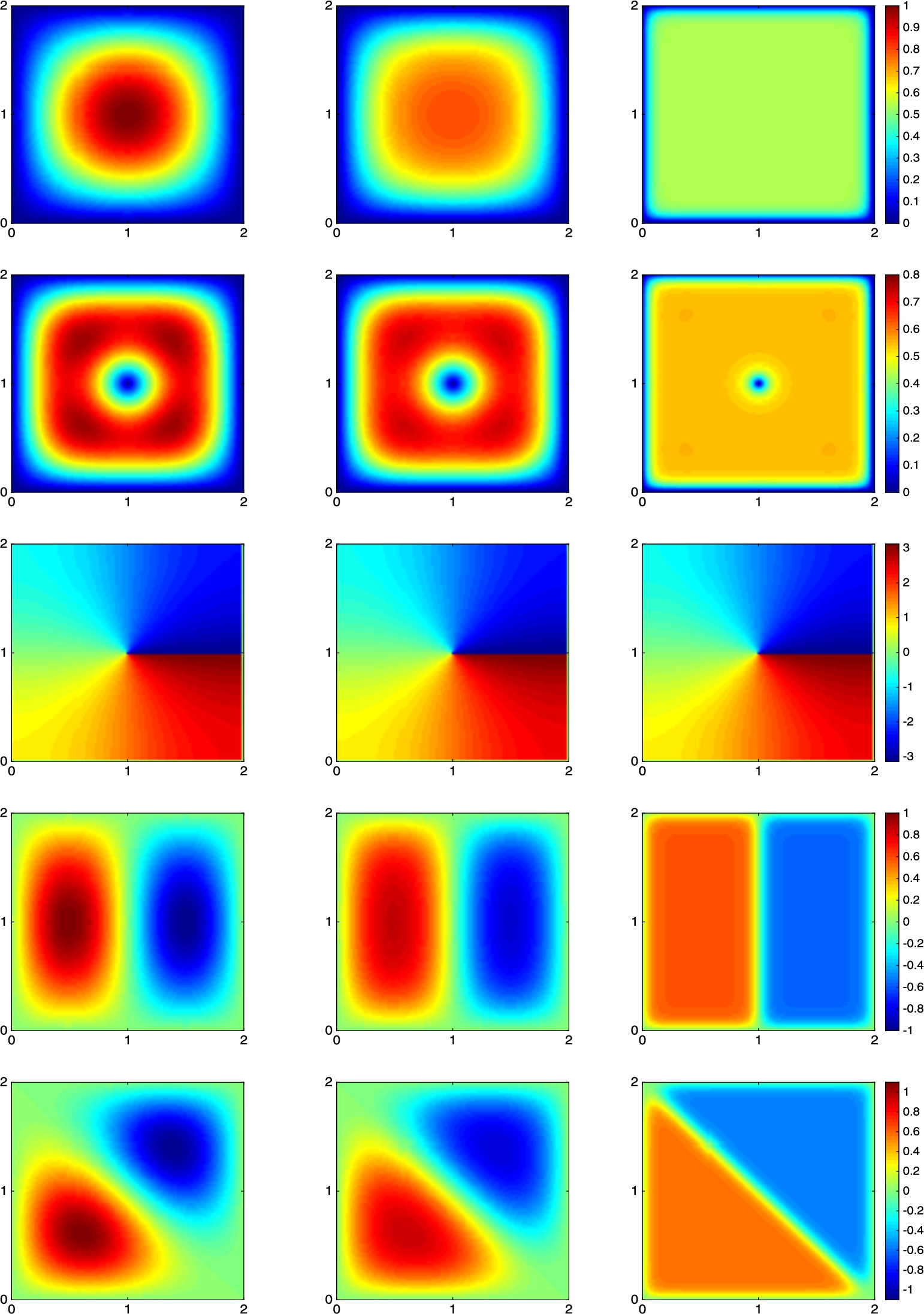
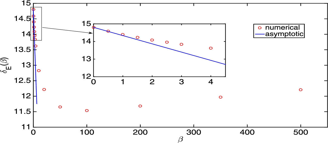
Again, to verify numerically our asymptotic results in Proposition 2.2, Fig. 6 plots the ground state $ϕ_{g}^{β}$ , the first excited state $ϕ_{1}^{β} = ϕ_{1, v}^{β}$ , and other excited states $ϕ_{1, x}^{β}$ and $ϕ_{1, c}^{β}$ , of the GPE in 2D with $Ω = {(0, 2)}^{2}$ and a box potential for different $β ⩾ 0$ , which were obtained numerically via the Backward Euler finite difference method [7–10]. Figure 7 depicts the energy $E_{g} (β) = E (ϕ_{g}^{β}) < E_{1} (β) = E (ϕ_{1}^{β} = ϕ_{1, v}^{β}) < E (ϕ_{1, x}^{β}) < E (ϕ_{1, c}^{β})$ for different $β ⩾ 0$ and the corresponding fundamental gaps in energy, and Fig. 8 shows the fundamental gaps in energy of GPE in 3D with $Ω = {(0, 1)}^{3}$ and a box potential. In addition, Fig. 9 depicts the fundamental gaps in energy of GPE in 2D with $Ω = B_{1} (0) = {x | | x | < 1}$ and a box potential.

Fig. 6.

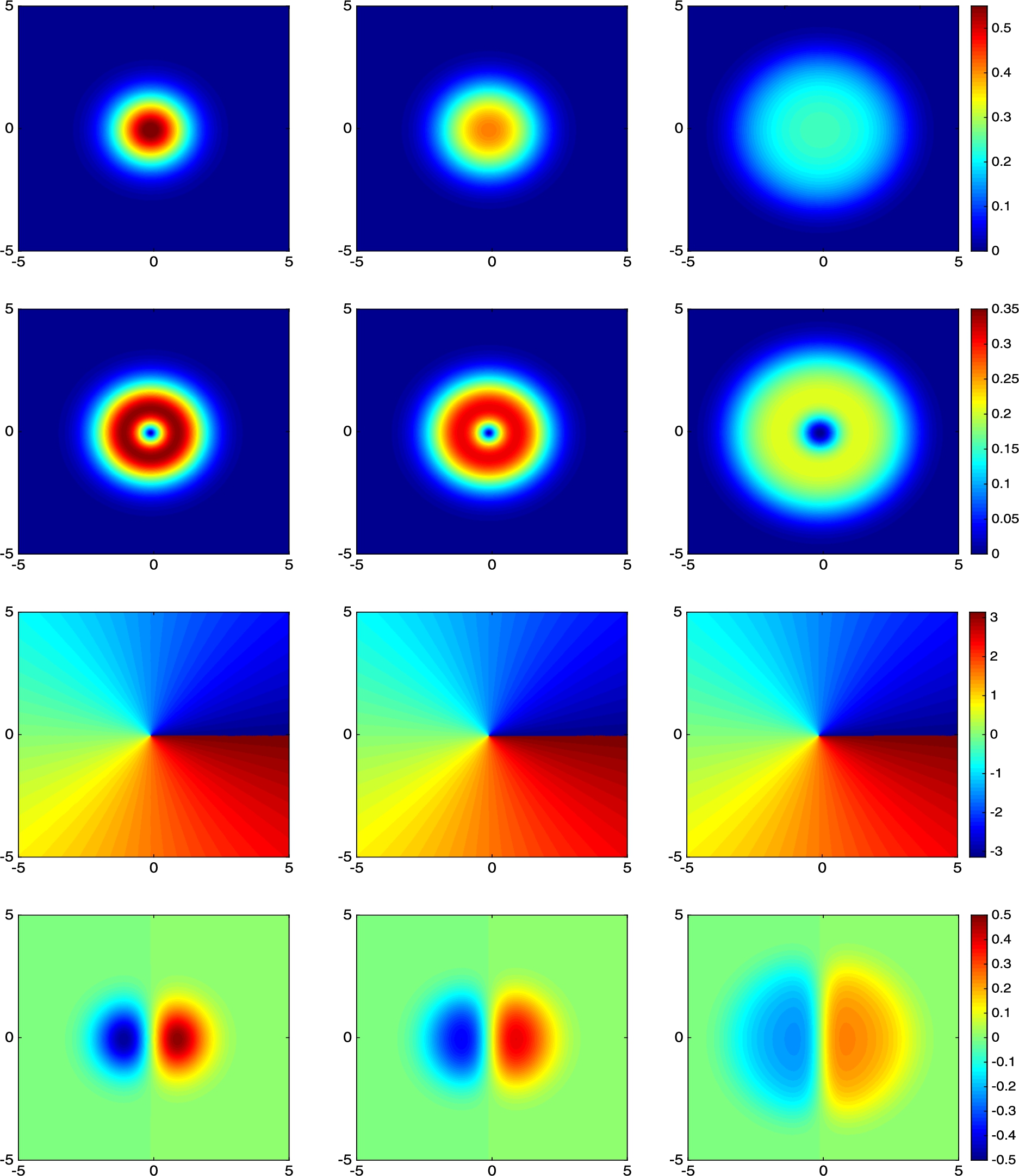
Ground states $ϕ_{g}^{β}$ (top row), first excited states – vortex solution $| ϕ_{1}^{β} = ϕ_{1, v}^{β} |$ (second row), excited states in the $x_{1}$ -direction $ϕ_{1, x}^{β}$ (fourth row) and excited states in the diagonal direction $ϕ_{1, c}^{β}$ (fifth row) for $β = 0$ (left column), $β = 10$ (middle column) and $β = 500$ (right column). Here the phase of the vortex solution – first excited state – is displayed in the third row.

Fig. 7.

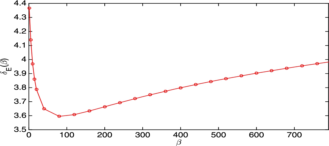
Energy $E_{g} (β) : = E (ϕ_{g}^{β}) < E_{1} (β) : = E (ϕ_{1}^{β} = ϕ_{1, v}^{β}) < E_{2} (β) : = E (ϕ_{1, x_{1}}^{β}) = E (ϕ_{1, x_{2}}^{β}) < E_{3} (β) : = E (ϕ_{1, c}^{β})$ of GPE in 2D under a box potential with $Ω = {(0, 2)}^{2}$ for different $β ⩾ 0$ (top) and the fundamental gaps in energy $δ_{E} (β)$ (bottom). Here a band crossing in energy happens at $β = 0$ for the excited states (cf. top).

Fig. 8.

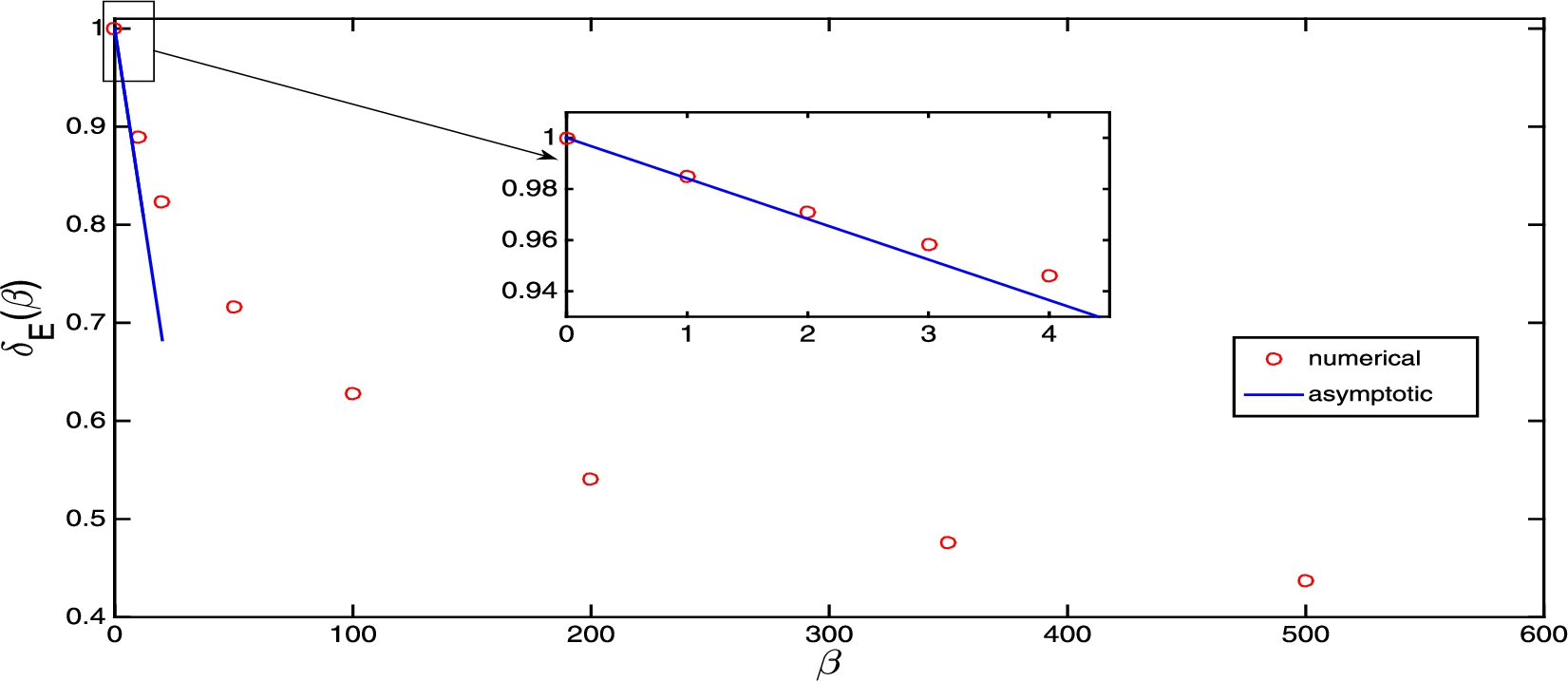
The fundamental gaps in energy of GPE in 3D under a box potential with $Ω = {(0, 1)}^{3}$ .

Fig. 9.

The fundamental gaps in energy of GPE under a box potential with $Ω = B_{1} (0)$ . It is obviously that the fundamental gap is larger than the lower bound proposed in the gap conjecture (1.13), which is $\frac{π^{2}}{2 D^{2}} \approx 1.234$ .

Based on the asymptotic results in Proposition 2.2 and the above numerical results as well as additional extensive numerical results not shown here for brevity [33], we speculate the gap conjecture (1.13).

3. Fundamental gaps of GPE in the whole space

In this section, we obtain asymptotically the fundamental gaps of the GPE (1.6) in the whole space under a harmonic potential and numerically under general potentials growing at least quadratically in the far field. Based on the results, we formulate a novel gap conjecture for this case. Here we take $Ω = R^{d}$ and denote $V_{h} (x) = \frac{1}{2} \sum_{j = 1}^{d} γ_{j}^{2} x_{j}^{2}$ satisfying $0 < γ_{1} ⩽ γ_{2} ⩽ \dots ⩽ γ_{d}$ .

3.1. Non-degenerate case, i.e. $dim (W_{1}) = 1$

We first consider the special case by taking $V (x) = V_{h} (x)$ satisfying $d = 1$ or $γ_{1} < γ_{2}$ when $d ⩾ 2$ . For simplicity, we define $\begin{matrix} (3.1) & B_{0} = \prod_{j = 1}^{d} \sqrt{\frac{γ_{j}}{2 π}}, B_{1} = \frac{1}{2} \sum_{j = 1}^{d} γ_{j}, B_{2} = \prod_{j = 1}^{d} γ_{j}, C_{d} = \{\begin{matrix} 2, & d = 1, \\ π, & d = 2, \\ \frac{4 π}{3}, & d = 3 . \end{matrix} \end{matrix}$

In this scenario, when $β = 0$ , all eigenfunctions can be obtained via the Hermite functions [13,14]. Thus the ground state $ϕ_{g}^{0} (x)$ and the first excited state $ϕ_{1}^{0} (x)$ can be given explicitly as [13,14] $\begin{matrix} (3.2) & ϕ_{g}^{0} (x) = \prod_{j = 1}^{d} {(\frac{γ_{j}}{π})}^{\frac{1}{4}} e^{- \frac{γ_{j} x_{j}^{2}}{2}}, ϕ_{1}^{0} (x) = \sqrt{2 γ_{1}} x_{1} \prod_{j = 1}^{d} {(\frac{γ_{j}}{π})}^{\frac{1}{4}} e^{- \frac{γ_{j} x_{j}^{2}}{2}}, x \in R^{d} . \end{matrix}$

Lemma 3.1.
In the weakly repulsive interaction regime, i.e. $0 < β ≪ 1$ , we have $\begin{array}{l} (3.3) & E_{g} (β) = B_{1} + \frac{B_{0}}{2} β + o (β), μ_{g} (β) = B_{1} + B_{0} β + o (β), \\ (3.4) & E_{1} (β) = γ_{1} + B_{1} + \frac{3 B_{0}}{8} β + o (β), μ_{1} (β) = γ_{1} + B_{1} + \frac{3 B_{0}}{4} β + o (β) . \end{array}$
Proof.
When $0 < β ≪ 1$ , we can approximate the ground state $ϕ_{g}^{β} (x)$ and the first excited state $ϕ_{1}^{β} (x)$ by $ϕ_{g}^{0} (x)$ and $ϕ_{1}^{0} (x)$ , respectively. Thus we have $\begin{matrix} (3.5) & ϕ_{g}^{β} (x) \approx ϕ_{g}^{0} (x), ϕ_{1}^{β} (x) \approx ϕ_{1}^{0} (x), x \in R^{d} . \end{matrix}$ Plugging (3.5) into (1.7) and (1.8), after a detailed computation which is omitted here for brevity [33], we can obtain (3.3) and (3.4). □
Lemma 3.2.
In the strongly repulsive interaction regime, i.e. $β ≫ 1$ , we have $\begin{array}{l} (3.6) & μ_{g} (β) \approx μ_{g}^{TF} = \frac{1}{2} {(\frac{(d + 2) B_{2} β}{C_{d}})}^{\frac{2}{d + 2}}, μ_{1} (β) \approx μ_{1}^{MA} = μ_{g}^{TF} + \frac{\sqrt{2}}{2} γ_{1} + o (1), \\ (3.7) & E_{g} (β) = \frac{2 + d}{4 + d} μ_{g}^{TF} + o (1), E_{1} (β) = E_{g} (β) + \frac{\sqrt{2}}{2} γ_{1} + o (1), β ≫ 1 . \end{array}$
Proof.
When $β ≫ 1$ , the ground and first excited states can be approximated by the TF approximations and/or uniformly accurate matched asymptotic approximations. For $d = 1$ and $V (x) = \frac{γ^{2} x^{2}}{2}$ , these approximations have been given explicitly and verified numerically in the literature [10,11,13,14], and the results can be extended to d dimensions ( $d = 1, 2, 3$ ) as $\begin{array}{l} (3.8) & ϕ_{g}^{β} (x) \approx ϕ_{g}^{TF} (x) = \sqrt{\frac{{(μ_{g}^{TF} - V (x))}_{+}}{β}}, x \in R^{d}, \\ (3.9) & ϕ_{1}^{β} (x) \approx ϕ_{1}^{MA} (x) = \{\begin{matrix} \sqrt{\frac{g_{1} (x)}{β}} + \sqrt{\frac{g_{2} (x)}{β}} [tanh (x_{1} \sqrt{g_{2} (x)}) - 1], & g_{1} (x) ⩾ 0 and x_{1} ⩾ 0, \\ - \sqrt{\frac{g_{1} (x)}{β}} + \sqrt{\frac{g_{2} (x)}{β}} [1 + tanh (x_{1} \sqrt{g_{2} (x)})], & g_{1} (x) ⩾ 0 and x_{1} < 0, \\ 0, & otherwise, \end{matrix} \end{array}$ where ${(f)}_{+} : = max {f, 0}$ , $g_{1} (x) = μ_{1}^{MA} - \frac{1}{2} \sum_{j = 1}^{d} γ_{j}^{2} x_{j}^{2}$ and $g_{2} (x) = μ_{1}^{MA} - \frac{1}{2} \sum_{j = 2}^{d} γ_{j}^{2} x_{j}^{2}$ , and $μ_{g}^{TF}$ and $μ_{1}^{MA}$ can be obtained via the normalization condition (1.4). Inserting (3.8) and (3.9) into (1.7), after a detailed computation which is omitted here for brevity [33], we get (3.7). □

From Lemmas 3.1 and 3.2, we have asymptotic results for the fundamental gaps.
Proposition 3.1 (For GPE under a harmonic potential in non-degenerate case).

When $V (x) = V_{h} (x)$ satisfying $d = 1$ or $γ_{1} < γ_{2}$ when $d ⩾ 2$ , i.e. GPE with a harmonic potential, we have $\begin{matrix} (3.10) & δ_{E} (β) = \{\begin{matrix} γ_{1} - \frac{B_{0}}{8} β + o (β), \\ \frac{\sqrt{2}}{2} γ_{1} + o (1), \end{matrix} δ_{μ} (β) = \{\begin{matrix} γ_{1} - \frac{B_{0}}{4} β + o (β), & 0 ⩽ β ≪ 1, \\ \frac{\sqrt{2}}{2} γ_{1} + o (1), & β ≫ 1 . \end{matrix} \end{matrix}$

Proof.
When $0 ⩽ β ≪ 1$ , subtracting (3.3) from (3.4), we obtain (3.10) in this parameter regime. Similarly, when $β ≫ 1$ , we get the result by recalling (3.6) and (3.7). □
Remark 3.1.
Similar to Lemma 2.2, when $β ≫ 1$ , by performing asymptotic expansion to the next order, we can obtain $\begin{array}{l} (3.11) & δ_{E} (β) = \frac{\sqrt{2}}{2} γ_{1} + \frac{γ_{1}^{2} {(d + 2)}^{\frac{d}{d + 2}}}{4} {(\frac{C_{d}}{B_{2} β})}^{\frac{2}{d + 2}} + o (β^{- \frac{2}{d + 2}}), β ≫ 1, \\ (3.12) & δ_{μ} (β) = \frac{\sqrt{2}}{2} γ_{1} + \frac{γ_{1}^{2} d {(d + 2)}^{- \frac{2}{d + 2}}}{4} {(\frac{C_{d}}{B_{2} β})}^{\frac{2}{d + 2}} + o (β^{- \frac{2}{d + 2}}), β ≫ 1 . \end{array}$

Fig. 10.
Ground states (left) and first excited states (right) of GPE in 1D with a harmonic potential $V (x) = x^{2} / 2$ (dot line) for different $β ⩾ 0$ .

Fig. 11.
Energy $E_{g} (β) : = E (ϕ_{g}^{β}) < E_{1} (β) : = E (ϕ_{1}^{β} = ϕ_{1, x}^{β}) < E_{2} (β) : = E (ϕ_{1, y}^{β})$ of GPE in 2D under a harmonic potential with $γ_{1} = 1 < γ_{2} = 2$ for different $β ⩾ 0$ .

Fig. 12.
Fundamental gaps in energy of GPE with a harmonic potential in 1D with $γ_{1} = 1$ (top), in 2D with $γ_{1} = 1 < γ_{2} = 2$ (middle), and in 3D with $γ_{1} = 1 < γ_{2} = γ_{3} = 2$ (bottom).

Again, to verify numerically our asymptotic results in Proposition 3.1, Figure 10 shows the ground and first excited states of GPE in 1D with $γ_{1} = 1$ for different $β ⩾ 0$ , which are obtained numerically via the Backward Euler finite difference method [7–10]. Figure 11 shows energy of the ground state, first excited state, i.e. excited state in the $x_{1}$ -direction, and excited states in the $x_{2}$ -direction and Fig. 12 depicts fundamental gaps in energy obtained numerically and asymptotically (cf. Eqs (3.11), (3.12) and (3.10)) in 1D, 2D and 3D. From Fig. 12, we can see that the asymptotic results in Proposition 3.1 are very accurate in both weakly repulsive interaction regime, i.e. $0 < β ≪ 1$ , and strongly repulsive interaction regime, i.e. $β ≫ 1$ . In addition, our numerical results suggest that both $δ_{E} (β)$ and $δ_{μ} (β)$ are decreasing functions for $β ⩾ 0$ (cf. Fig. 12).

Fig. 13.
Fundamental gaps in energy (left) and chemical potential (right) of GPE in 1D with $V (x) = \frac{x^{2}}{2} + V_{0} cos (k x)$ satisfying $V_{0} k^{2} = 0.5$ for different β, $V_{0}$ and k.

Again, for general external potentials, the ground and first excited states as well as their energy and chemical potential can be computed numerically via the Backward Euler finite difference method [7–10] if the external potential is symmetric and via the method proposed in [15] with spectral discretization in space if the external potential is asymmetric. Figure 13 depicts fundamental gaps in energy and chemical potential of GPE in 1D with $V (x) = \frac{x^{2}}{2} + V_{0} cos (k x)$ for different β, $V_{0}$ and k, and Fig. 14 shows the fundamental gaps of GPE in 1D with different convex trapping potentials growing at least quadratically in the far field for different $β ⩾ 0$ .

Fig. 14.
Fundamental gaps in energy (left) and chemical potential (right) of GPE in 1D with (I) $V (x) = \frac{x^{2}}{2} + 0.5 sin (x)$ , (II) $V (x) = \frac{x^{2}}{4} - x$ , (III) $V (x) = \frac{x^{2}}{4} + \frac{x^{4}}{100} + x$ for different $β ⩾ 0$ .
3.2. Degenerate case, i.e. $dim (W_{1}) ⩾ 2$

We first consider a special case by taking $V (x) = V_{h} (x)$ satisfying $d ⩾ 2$ and $γ_{1} = γ_{2} : = γ$ . In this case, the approximations to the ground states and their energy and chemical potential are the same as those in the previous subsection by letting $γ_{2} \to γ_{1} = γ$ . Therefore, we only need to focus on the approximations to the first excited states, which are completely different with those in the non-degenerate case.

Lemma 3.3.
For weakly interaction regime, i.e. $0 < β ≪ 1$ , we have for $d ⩾ 2$ $\begin{array}{l} (3.13) & E_{1} (β) & = \frac{3 γ}{2} + \frac{B_{0} d}{8} β + o (β), μ_{1} (β) = \frac{3 γ}{2} + \frac{B_{0} d}{4} β + o (β) . \end{array}$
Proof.
For simplicity, we only present the 2D case and extension to 3D is straightforward. Denote $\begin{matrix} (3.14) & ϕ_{g}^{0} (x) = {(\frac{γ}{π})}^{\frac{1}{4}} e^{- \frac{γ x^{2}}{2}}, ϕ_{1}^{0} (x) = \sqrt{2 γ} {(\frac{γ}{π})}^{\frac{1}{4}} x e^{- \frac{γ x^{2}}{2}} . \end{matrix}$ When $d = 2$ and $β = 0$ , it is easy to see that $φ_{1} (x) : = ϕ_{1}^{0} (x_{1}) ϕ_{g}^{0} (x_{2})$ and $φ_{2} (x) : = ϕ_{g}^{0} (x_{1}) ϕ_{1}^{0} (x_{2})$ are two linearly independent orthonormal first excited states. In fact, $W_{1} = span {φ_{1}, φ_{2}}$ . In order to find an appropriate approximation of the first excited state when $0 < β ≪ 1$ , we take an ansatz $\begin{matrix} (3.15) & φ_{a, b} (x) = a φ_{1} (x) + b φ_{2} (x), x \in R^{2}, \end{matrix}$ where $a, b \in C$ satisfying $| a |^{2} + | b |^{2} = 1$ implies $‖ φ_{a, b} ‖_{2} = 1$ . Then a and b can be determined by minimizing $E (φ_{a, b})$ . Plugging (3.15) into (1.8), we have for $β ⩾ 0$ $\begin{array}{l} (3.16) & E (φ_{a, b}) = 3 γ + \frac{γ β}{16 π} [{| a^{2} + b^{2} |}^{2} + 2 {(| a |^{2} + | b |^{2})}^{2}] ⩾ 3 γ + \frac{γ β}{8 π}, \end{array}$ which is minimized when $a^{2} + b^{2} = 0$ , i.e. $a = \pm i b$ . By taking $a = 1 / \sqrt{2}$ and $b = i / \sqrt{2}$ , we get an approximation of the first excited state as [16,22,35] $\begin{matrix} (3.17) & ϕ_{1}^{β} (x) \approx ϕ_{1, v} (x) = \frac{γ}{\sqrt{π}} (x_{1} + i x_{2}) e^{- \frac{γ (x_{1}^{2} + x_{2}^{2})}{2}} = \frac{γ}{\sqrt{π}} r e^{- \frac{γ r^{2}}{2}} e^{i θ}, \end{matrix}$ where $(r, θ)$ is the polar coordinate. Substituting (3.17) into (1.8) and (1.7), we get (3.13). □
Lemma 3.4.
For the 2D case with strongly repulsive interaction, i.e. $d = 2$ and $β ≫ 1$ , we have $\begin{matrix} (3.18) & E_{1} (β) = E_{g}^{TF} + \frac{γ}{2} \sqrt{\frac{π}{β}} ln (β) + O (β^{- \frac{1}{2}}), μ_{1} (β) = μ_{g}^{TF} + \frac{γ}{4} \sqrt{\frac{π}{β}} ln (β) + O (β^{- \frac{1}{2}}), \end{matrix}$ where $μ_{g}^{TF}$ is given in ( 3.6 ) and $E_{g}^{TF} = \frac{2 + d}{4 + d} μ_{g}^{TF}$ .
Proof.
From Lemma 3.3, when $0 < β ≪ 1$ , the first excited state needs to be taken as a vortex-type solution. By assuming that there is no band crossing when $β > 0$ , the first excited state can be well approximated by the vortex-type solution when $β ≫ 1$ too. Thus when $β ≫ 1$ , we approximate the first excited state via a matched asymptotic approximation.
In the outer region, i.e. $| x | > o (1)$ , it is approximated by the TF approximation as $\begin{matrix} (3.19) & ϕ_{1}^{β} (x) \approx ϕ^{out} (x) \approx \sqrt{\frac{{(2 μ_{1} - γ^{2} r^{2})}_{+}}{2 β}}, r > o (1), \end{matrix}$ where $μ = μ_{1} (β)$ is the chemical potential of the first excited state.

In the inner region near the origin, i.e. $| x | ≪ 1$ , it is approximated by a vortex solution with winding number $m = 1$ as $\begin{matrix} (3.20) & ϕ_{1}^{β} (x) \approx ϕ^{in} (x) = \sqrt{\frac{μ_{1}}{β}} f (r) e^{i θ}, | x | ≪ 1 . \end{matrix}$ Substituting (2.32) into (1.6), we get the equation for $f (r)$ $\begin{matrix} (3.21) & - \frac{1}{2} f^{″} (r) - \frac{1}{2 r} f^{'} (r) + \frac{1}{2 r^{2}} f (r) + \frac{γ^{2} r^{2}}{2} f (r) + μ_{1} f^{3} (r) = μ_{1} f (r), r > 0, \end{matrix}$ with BC $f (0) = 0$ . When $β ≫ 1$ and $0 ⩽ r ≪ 1$ , by dropping the terms $- \frac{1}{2} f^{″} (r)$ and $\frac{γ^{2} r^{2}}{2} f (r)$ in (3.21) and then solving it analytically with the far field limit ${lim}_{r \to + \infty} f (r) = 1$ , we get (2.34). Combining the outer and inner approximations via the matched asymptotic technique, we obtain an asymptotic approximation of the density of the first excited state as $\begin{matrix} (3.22) & ρ_{1}^{β} (x) : = {| ϕ_{1}^{β} (x) |}^{2} \approx \frac{2 μ_{1} r^{2}}{1 + 2 μ_{1} r^{2}} \frac{{(2 μ_{1} - γ^{2} r^{2})}_{+}}{2 β}, r ⩾ 0 . \end{matrix}$ Substituting (3.22) into the normalization condition $‖ ϕ_{1}^{β} ‖_{2} = 1$ and (1.7), a detailed computation gives the approximation of the chemical potential and energy in (3.18). The details of the computation are omitted here for brevity [33]. □

Fig. 15.
Ground state $ϕ_{g}^{β}$ (top row), first excited state – vortex solution $| ϕ_{1}^{β} = ϕ_{1, v}^{β} |$ (second row) and higher excited state in $x_{1}$ -direction $ϕ_{1, x}^{β}$ (bottom row) of GPE in 2D with a harmonic potential ( $γ = 1$ ) for $β = 0$ (left column), $β = 10$ (middle column) and $β = 100$ (right column). The phase of the first excited state $ϕ_{1}^{β} = ϕ_{1, v}^{β}$ is displayed in the third row.

Fig. 16.
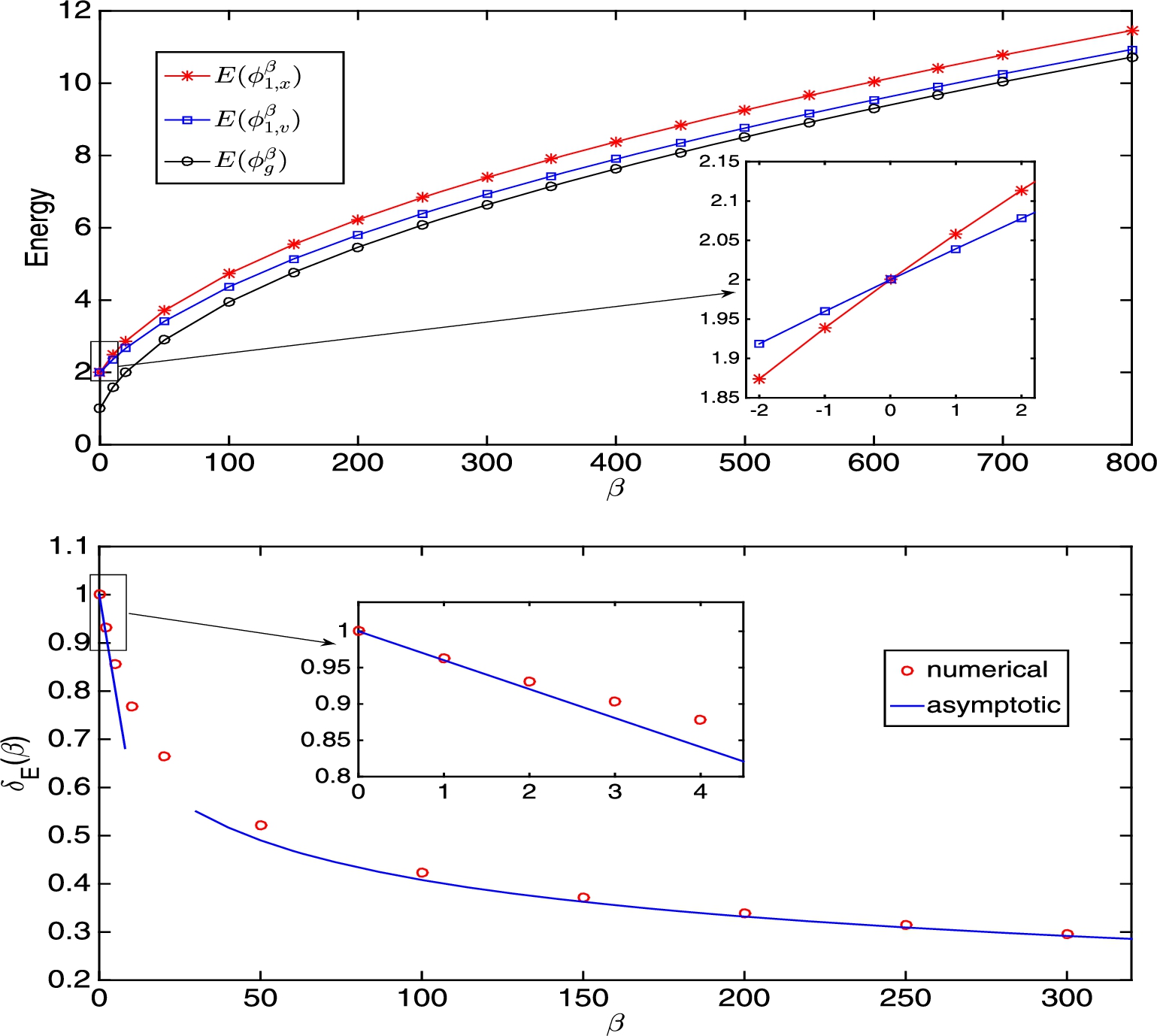
Energy $E_{g} (β) : = E (ϕ_{g}^{β}) < E_{1} (β) : = E (ϕ_{1}^{β} = ϕ_{1, v}^{β}) < E_{2} (β) : = E (ϕ_{1, x_{1}}^{β}) = E (ϕ_{1, x_{2}}^{β})$ of GPE in 2D under the harmonic potential $V (x) = \frac{x_{1}^{2} + x_{2}^{2}}{2}$ for different $β ⩾ 0$ (top) and the fundamental gap in energy $δ_{E} (β)$ for different $β ⩾ 0$ (bottom).

Fig. 17.
The fundamental gaps in energy of GPE in 3D under a harmonic potential $V (x) = (x_{1}^{2} + x_{2}^{2} + x_{3}^{2}) / 2$ for different $β ⩾ 0$ .

From Lemmas 3.3–3.4, we have asymptotic results for the fundamental gaps.
Proposition 3.2 (For GPE under a harmonic potential in degenerate case).

When $V (x) = V_{h} (x)$ with $d ⩾ 2$ and $γ_{1} = γ_{2} : = γ$ , i.e. GPE with a harmonic potential, we have

when $0 ⩽ β ≪ 1$ and $d ⩾ 2$ $\begin{matrix} (3.23) & δ_{E} (β) = γ - \frac{(4 - d) B_{0}}{8} β + o (β), δ_{μ} (β) = γ - \frac{(4 - d) B_{0}}{4} β + o (β); \end{matrix}$

when $β ≫ 1$ and $d = 2$ , $\begin{matrix} (3.24) & δ_{E} (β) = \frac{γ_{1}}{2} \sqrt{\frac{π}{β}} ln (β) + o (\frac{ln (β)}{\sqrt{β}}), δ_{μ} (β) = \frac{γ_{1}}{4} \sqrt{\frac{π}{β}} ln (β) + o (\frac{ln (β)}{\sqrt{β}}), \end{matrix}$ which implies $δ_{E} (β) \to 0$ and $δ_{μ} (β) \to 0$ as $β \to \infty$ .

Again, to verify numerically our asymptotic results in Proposition 3.2, Fig. 15 plots the ground state $ϕ_{g}^{β}$ , the first excited state $ϕ_{1}^{β} = ϕ_{1, v}^{β}$ , and the higher excited states $ϕ_{1, x}^{β}$ , of GPE in 2D with a harmonic potential ( $γ = 1$ ) for different $β ⩾ 0$ , which were obtained numerically via the Backward Euler finite difference method [7–10]. Figure 16 depicts the energy $E_{g} (β) = E (ϕ_{g}^{β}) < E_{1} (β) = E (ϕ_{1}^{β} = ϕ_{1, v}^{β}) < E (ϕ_{1, x}^{β})$ for different $β ⩾ 0$ and the corresponding fundamental gaps in energy, and Fig. 17 shows the fundamental gaps in energy of GPE in 3D with a harmonic potential. In addition, our numerical results suggest that both $δ_{E} (β)$ and $δ_{μ} (β)$ are decreasing functions for $β ⩾ 0$ (cf. Figs 16 and 17).

Based on the asymptotic results in Propositions 3.1 and 3.2 and the above numerical results as well as additional extensive numerical results not shown here for brevity [33], we speculate the following gap conjecture.

Gap Conjecture II (For GPE in whole space).

Suppose $Ω = R^{d}$ and the external potential $V (x)$ satisfies $D^{2} V (x) ⩾ γ_{1}^{2} I_{d}$ for $x \in R^{d}$ with $γ_{1} > 0$ a constant.

In the non-degenerate case, i.e. when $dim (W_{1}) = 1$ , we have $\begin{matrix} (3.25) & δ_{E}^{\infty} : = inf_{β ⩾ 0} δ_{E} (β) ⩾ \frac{\sqrt{2}}{2} γ_{1}, δ_{μ}^{\infty} : = inf_{β ⩾ 0} δ_{μ} (β) ⩾ \frac{\sqrt{2}}{2} γ_{1} . \end{matrix}$

In the degenerate case, i.e. when $dim (W_{1}) ⩾ 2$ , we have $\begin{matrix} (3.26) & δ_{E} (β) ⩾ γ_{1} - C_{1} β, δ_{μ} (β) ⩾ γ_{1} - C_{2} β, 0 ⩽ β ≪ 1, \end{matrix}$ where $C_{1} > 0$ and $C_{2} > 0$ are two constants independent of β. In addition, if the potential $V (x)$ is a harmonic-type potential, we have ${lim}_{β \to + \infty} δ_{E} (β) = 0$ and ${lim}_{β \to + \infty} δ_{μ} (β) = 0$ .

4. Extensions to other BCs

In this section, we study the fundamental gaps of GPE on bounded domains with either periodic BC or homogeneous Neumann BC.

4.1. Results for the periodic BC

Take $Ω = Ω_{0}$ and assume that ϕ satisfies the periodic BC. When $d = 1$ , it corresponds to a BEC on a ring [7]; and when $d = 2$ , it corresponds to a BEC on a torus. In this case, the ground state $ϕ_{g}^{β}$ is defined the same as in (1.9) provided that the set S is replaced by $S = {ϕ | ‖ ϕ ‖_{2}^{2} : = \int_{Ω} | ϕ (x) |^{2} d x = 1, E (ϕ) < \infty, ϕ is periodic on \partial Ω}$ , and the first excited state $ϕ_{1}^{β}$ and the eigenspace $W_{1}$ are defined similarly. We have the following results for the energy and chemical potential of the ground and first excited states.

Lemma 4.1.
Assume $V (x) \equiv 0$ , for all $β ⩾ 0$ and $d = 1, 2, 3$ , we have $\begin{array}{l} (4.1) & \begin{matrix} E_{g} (β) = \frac{A_{0}^{2}}{2} β, μ_{g} (β) = A_{0}^{2} β, \\ E_{1} (β) = \frac{2 π^{2}}{L_{1}^{2}} + \frac{A_{0}^{2}}{2} β, μ_{1} (β) = \frac{2 π^{2}}{L_{1}^{2}} + A_{0}^{2} β . \end{matrix} \end{array}$
Proof.
For any $ϕ \in S$ , the Cauchy–Schwarz inequality implies that $\begin{matrix} (4.2) & 1 = ‖ ϕ ‖_{2}^{4} = {(\int_{Ω} | ϕ |^{2} d x)}^{2} ⩽ \int_{Ω} | ϕ |^{4} d x \int_{Ω} 1 d x = \frac{1}{A_{0}^{2}} \int_{Ω} | ϕ |^{4} d x . \end{matrix}$ Thus, for all $β ⩾ 0$ and any $ϕ \in S$ , we have $\begin{matrix} (4.3) & E (ϕ) = \int_{Ω} [\frac{1}{2} | \nabla ϕ |^{2} + \frac{β}{2} | ϕ |^{4}] d x ⩾ \frac{β}{2} A_{0}^{2} = \frac{β}{2} \int_{Ω} | A_{0} |^{4} d x = E (ϕ \equiv A_{0}) . \end{matrix}$ Therefore, for all $β ⩾ 0$ , we have $\begin{matrix} (4.4) & ϕ_{g}^{β} (x) \equiv ϕ_{g}^{0} (x) : = A_{0}, x \in \overline{Ω} . \end{matrix}$ Plugging (4.4) into (1.8) and (1.7) and noticing $V (x) \equiv 0$ , we obtain the first two equalities in (4.1).

As for the first excited state, for simplicity, we only present 1D case and extensions to 2D and 3D are straightforward. When $d = 1$ and $β = 0$ , it is easy to see that $φ_{1} (x) : = \sqrt{2} A_{0} cos (2 π x / L_{1})$ and $φ_{2} (x) : = \sqrt{2} A_{0} sin (2 π x / L_{1})$ are two linearly independent orthonormal first excited states. In fact, in this case, $W_{1} = span {φ_{1}, φ_{2}}$ . In order to find an appropriate approximation of the first excited state when $0 < β ≪ 1$ , we take an ansatz $\begin{matrix} (4.5) & φ_{a, b} (x) = a φ_{1} (x) + b φ_{2} (x), 0 ⩽ x ⩽ L_{1}, \end{matrix}$ where $a, b \in C$ satisfying $| a |^{2} + | b |^{2} = 1$ implies $‖ φ_{a, b} ‖_{2} = 1$ . Then a and b can be determined by minimizing $E (φ_{a, b})$ . Plugging (4.5) into (1.8), we have for $β ⩾ 0$ $\begin{array}{l} (4.6) & E (φ_{a, b}) = \frac{2 π^{2}}{L_{1}^{2}} + \frac{β}{4 L_{1}} [2 {(| a |^{2} + | b |^{2})}^{2} + {| a^{2} + b^{2} |}^{2}] ⩾ \frac{2 π^{2}}{L_{1}^{2}} + \frac{β}{2 L_{1}}, \end{array}$ which is minimized when $a^{2} + b^{2} = 0$ , i.e. $a = \pm i b$ . By taking $a = 1 / \sqrt{2}$ and $b = i / \sqrt{2}$ , we get an approximation of the first excited state as $\begin{matrix} (4.7) & ϕ_{1}^{β} (x) \approx ϕ_{1}^{0} (x) : = A_{0} e^{i 2 π x / L_{1}}, 0 ⩽ x ⩽ L_{1} . \end{matrix}$ Similar to (4.2) and (4.3), we can prove rigorously that for all $β ⩾ 0$ $\begin{matrix} (4.8) & ϕ_{1}^{β} (x) \equiv ϕ_{1}^{0} (x) = A_{0} e^{i 2 π x / L_{1}}, 0 ⩽ x ⩽ L_{1} . \end{matrix}$ Plugging (4.8) into (1.8) and (1.7), we obtain the last two equalities in (4.1). □

From (4.1), it is straightforward to have (with the proof omitted here for brevity).
Proposition 4.1 (For GPE on a bounded domain with periodic BC).

Assume $V (x) \equiv 0$ , we have $\begin{matrix} (4.9) & δ_{E} (β) = δ_{μ} (β) = \frac{2 π^{2}}{L_{1}^{2}}, β ⩾ 0 . \end{matrix}$

Based on the above analytical results and extensive numerical results not shown here for brevity [33], we speculate the following gap conjecture.

Gap Conjecture III (For GPE on a bounded domain with periodic BC).

Suppose $Ω = Ω_{0}$ and the external potential $V (x)$ is convex and periodic, we speculate the following gap conjecture $\begin{matrix} (4.10) & δ_{E}^{\infty} : = inf_{β ⩾ 0} δ_{E} (β) ⩾ \frac{2 π^{2}}{D^{2}}, δ_{μ}^{\infty} : = inf_{β ⩾ 0} δ_{μ} (β) ⩾ \frac{2 π^{2}}{D^{2}} . \end{matrix}$

4.2. Results for homogeneous Neumann BC

Assume that $Ω \subset R^{d}$ is a bounded domain and ϕ satisfies the homogeneous Neumann BC, i.e. $\partial_{n} ϕ |_{\partial Ω} = 0$ with n the unit outward normal vector. In this case, the ground state $ϕ_{g}^{β}$ is defined the same as in (1.9) provided that the set S is replaced by $S = {ϕ | ‖ ϕ ‖_{2}^{2} : = \int_{Ω} | ϕ (x) |^{2} d x = 1, E (ϕ) < \infty, \partial_{n} ϕ |_{\partial Ω} = 0}$ , and the first excited state $ϕ_{1}^{β}$ and the eigenspace $W_{1}$ are defined similarly.

Similar to Lemma 4.1 (with the proof omitted here for brevity), we have

Lemma 4.2.
For the ground state $ϕ_{g}^{β}$ , we have for $β ⩾ 0$ $\begin{array}{l} (4.11) & ϕ_{g}^{β} (x) = ϕ_{g}^{0} (x) \equiv \frac{1}{\sqrt{\int_{Ω} 1 d x}} : = {\tilde{A}}_{0}, x \in \overline{Ω}; E_{g} (β) = \frac{{\tilde{A}}_{0}^{2}}{2} β, μ_{g} (β) = {\tilde{A}}_{0}^{2} β . \end{array}$

However, for the first excited state, we first consider a special case by taking $Ω = Ω_{0}$ and distinguish two different cases: (i) non-degenerate case $d = 1$ or $L_{1} > L_{2}$ when $d ⩾ 2$ ( $\Leftrightarrow dim (W_{1}) = 1$ ); and (ii) degenerate case $L_{1} = L_{2}$ and $d ⩾ 2$ ( $\Leftrightarrow dim (W_{1}) ⩾ 2$ ).
Lemma 4.3.
Assume $Ω = Ω_{0}$ satisfying $d = 1$ or $L_{1} > L_{2}$ when $d ⩾ 2$ , i.e. non-degenerate case, we have
in the weakly repulsive interaction regime, i.e. $0 < β ≪ 1$ , $\begin{array}{l} (4.12) & E_{1} (β) = \frac{π^{2}}{2 L_{1}^{2}} + \frac{3 A_{0}^{2}}{4} β + o (β), μ_{1} (β) = \frac{π^{2}}{2 L_{1}^{2}} + \frac{3 A_{0}^{2}}{2} β + o (β); \end{array}$

in the strongly repulsive interaction regime, i.e. $β ≫ 1$ , $\begin{array}{l} (4.13) & \begin{matrix} E_{1} (β) = \frac{A_{0}^{2}}{2} β + \frac{4 A_{0}}{3 L_{1}} β^{1 / 2} + \frac{2}{L_{1}^{2}} + o (1), \\ μ_{1} (β) = A_{0}^{2} β + \frac{2 A_{0}}{L_{1}} β^{1 / 2} + \frac{2}{L_{1}^{2}} + o (1) . \end{matrix} \end{array}$

Proof.
Here we only present the proof in 1D case and extension to high dimensions is similar to that in Lemma 2.3. When $d = 1$ and $β = 0$ , the first excited state can be taken as $ϕ_{1}^{0} (x) = \sqrt{2} A_{0} cos (π x / L_{1})$ for $x \in [0, L_{1}]$ . When $0 < β ≪ 1$ , we can approximate $ϕ_{1}^{β} (x)$ by $ϕ_{1}^{0} (x)$ , i.e. $\begin{matrix} (4.14) & ϕ_{1}^{β} (x) \approx ϕ_{1}^{0} (x) = \sqrt{2} A_{0} cos (π x / L_{1}), 0 ⩽ x ⩽ L_{1} . \end{matrix}$ Plugging (4.14) into (1.8) and (1.7) with $V (x) \equiv 0$ , we obtain (4.12). When $β ≫ 1$ , i.e. in strongly repulsive interaction regime, the first excited state can be approximated via the matched asymptotic method shown in [13,14] as $\begin{matrix} (4.15) & ϕ_{1}^{β} (x) \approx ϕ_{1}^{M A} (x) = \sqrt{\frac{μ_{1}^{M A}}{β}} tanh (\sqrt{μ_{1}^{M A}} (\frac{L_{1}}{2} - x)), 0 ⩽ x ⩽ L_{1} . \end{matrix}$ Substituting (4.15) into the normalization condition (1.4) and (1.7), we obtain (4.13), while the detailed computation is omitted here for brevity [33]. □
Lemma 4.4.
Assume $Ω = Ω_{0}$ satisfying $L_{1} = L_{2} : = L$ and $d ⩾ 2$ , i.e. degenerate case, we have
in the weakly repulsive interaction regime, i.e. $0 ⩽ β ≪ 1$ , $\begin{array}{l} (4.16) & E_{1} (β) = \frac{π^{2}}{2 L^{2}} + \frac{5 A_{0}^{2}}{8} β + o (β), μ_{1} (β) = \frac{π^{2}}{2 L^{2}} + \frac{5 A_{0}^{2}}{4} β + o (β); \end{array}$

in the strongly repulsive interaction regime, i.e. $β ≫ 1$ , and $d = 2$ , $\begin{array}{l} (4.17) & \begin{matrix} E_{1} (β) = \frac{β}{2 L^{2}} + \frac{π}{2 L^{2}} ln (β) + o (ln (β)), \\ μ_{1} (β) = \frac{β}{L^{2}} + \frac{π}{2 L^{2}} ln (β) + o (ln (β)) . \end{matrix} \end{array}$

Proof.
The proof is similar to that for Lemmas 2.4 and 2.5 in the box potential case and thus it is omitted here for brevity [33]. □

Lemmas 4.3 and 4.4 implies the following proposition about the fundamental gaps.
Proposition 4.2 (For GPE on a bounded domain with homogeneous Neumann BC).

Assume $Ω = Ω_{0}$ and $V (x) \equiv 0$ , we have

if $d = 1$ or $L_{1} > L_{2}$ when $d ⩾ 2$ , i.e. non-degenerate case, $\begin{array}{l} (4.18) & δ_{E} (β) = \{\begin{matrix} \frac{π^{2}}{2 L_{1}^{2}} + \frac{A_{0}^{2}}{4} β + o (β), \\ \frac{4 A_{0}}{3 L_{1}} β^{1 / 2} + \frac{2}{L_{1}^{2}} + o (1), \end{matrix} δ_{μ} (β) = \{\begin{matrix} \frac{π^{2}}{2 L_{1}^{2}} + \frac{A_{0}^{2}}{2} β + o (β), & 0 ⩽ β ≪ 1, \\ \frac{2 A_{0}}{L_{1}} β^{1 / 2} + \frac{2}{L_{1}^{2}} + o (1), & β ≫ 1; \end{matrix} \end{array}$

if $L_{1} = L_{2} : = L$ , i.e. degenerate case, with $0 ⩽ β ≪ 1$ and $d ⩾ 2$ , $\begin{matrix} (4.19) & δ_{E} (β) = \frac{π^{2}}{2 L^{2}} + \frac{β}{8 L^{2}} + o (β), δ_{μ} (β) = \frac{π^{2}}{2 L^{2}} + \frac{β}{4 L^{2}} + o (β) . \end{matrix}$

For the degenerate case with $β ≫ 1$ and $d = 2$ , $\begin{matrix} (4.20) & δ_{E} (β) = \frac{π}{2 L^{2}} ln (β) + o (ln (β)), δ_{μ} (β) = \frac{π}{2 L^{2}} ln (β) + o (ln (β)) . \end{matrix}$

The above asymptotic results have been verified numerically [33], which are omitted here to avoid this paper to be too long. In addition, our numerical results suggest that both $δ_{E} (β)$ and $δ_{μ} (β)$ are increasing functions for $β ⩾ 0$ [33].

Based on the above asymptotic results and numerical results not shown here for brevity [33], we speculate the following gap conjecture.

Gap Conjecture IV (For GPE on a bounded domain with homogeneous Neumann BC).

Suppose Ω is a convex bounded domain and the external potential $V (x)$ is convex, we speculate the following gap conjecture $\begin{matrix} (4.21) & δ_{E}^{\infty} : = inf_{β ⩾ 0} δ_{E} (β) ⩾ \frac{π^{2}}{2 D^{2}}, δ_{μ}^{\infty} : = inf_{β ⩾ 0} δ_{μ} (β) ⩾ \frac{π^{2}}{2 D^{2}} . \end{matrix}$

5. Conclusions

Fundamental gaps in energy and chemical potential of the Gross–Pitaevskii equation (GPE) with repulsive interaction were obtained asymptotically and computed numerically for different trapping potentials and a gap conjecture on fundamental gaps was formulated. In obtaining the approximation of the first excited state of GPE and the fundamental gaps, two different cases were identified in high dimensions ( $d ⩾ 2$ ), i.e. non-degenerate and degenerate cases which correspond to the dimensions $dim (W_{1}) = 1$ and $dim (W_{1}) ⩾ 2$ , respectively, with $W_{1}$ the eigenspace associated to the second smallest eigenvalue of the corresponding Schrödinger operator $H : = - \frac{1}{2} Δ + V (x)$ . Our asymptotic results were confirmed by numerical results. Rigorous mathematical justification for the fundamental gaps obtained asymptotically and numerically for the GPE in this paper is on-going. Finally, we remark here that the fundamental gaps in the degenerate case are the same as those in the non-degenerate case when one requires the solution ϕ of (1.6) to be real-valued function instead of complex-valued function.

Footnotes

Acknowledgements

This work was supported by Singapore Ministry of Education Academic Research Fund Tier 2 R-146-000-223-112.

References

M.H.

Anderson,

J.R.

Ensher,

M.R.

Matthews,

C.E.

Wieman and

E.A.

Cornell, Observation of Bose–Einstein condensation in a dilute atomic vapor, Science 269 (1995), 198–201. doi:10.1126/science.269.5221.198.

Andrews and

Clutterbuck, Proof of the fundamental gap conjecture, J. Amer. Math. Soc. 24 (2011), 899–916. doi:10.1090/S0894-0347-2011-00699-1.

Ashbaugh, The Fundamental Gap, Workshop on Low Eigenvalues of Laplace and Schrödinger Operators, American Institute of Mathematics, Palo Alto, California, 2006.

M.S.

Ashbaugh and

Benguria, Optimal lower bound for the gap between the first two eigenvalues of one-dimensional Schrödinger operators with symmetric single-well potentials, Proc. Amer. Math. Soc. 105 (1989), 419–424.

P.W.

Atkins, Physical Chemistry, Oxford University Press, 1978.

Bao, Mathematical models and numerical methods for Bose–Einstein condensation, in: Proceedings of the International Congress of Mathematicians (Seoul 20140), IV, 2014, pp. 971–996.

Bao and

Cai, Mathematical theory and numerical methods for Bose–Einstein condensation, Kinet. Relat. Models 6 (2012), 1–135. doi:10.3934/krm.2013.6.1.

Bao and

M.-H.

Chai, A uniformly convergent numerical method for singularly perturbed nonlinear eigenvalue problems, Commun. Comput. Phys. 4 (2008), 135–160.

Bao,

I.-L.

Chern and

F.Y.

Lim, Efficient and spectrally accurate numerical methods for computing ground and first excited states in Bose–Einstein condensates, J. Comput. Phys. 219 (2006), 836–854. doi:10.1016/j.jcp.2006.04.019.

10.

Bao and

Du, Computing the ground state solution of Bose–Einstein condensates by a normalized gradient flow, SIAM J. Sci. Comput. 25 (2004), 1674–1697. doi:10.1137/S1064827503422956.

11.

Bao,

Ge,

Jaksch,

P.A.

Markowich and

R.M.

Weishaeupl, Convergence rate of dimension reduction in Bose–Einstein condensates, Comput. Phys. Commun. 177 (2007), 832–850. doi:10.1016/j.cpc.2007.06.015.

12.

Bao,

Jaksch and

P.A.

Markowich, Numerical solution of the Gross–Pitaevskii equation for Bose–Einstein condensation, J. Comput. Phys. 187 (2003), 318–342. doi:10.1016/S0021-9991(03)00102-5.

13.

Bao and

F.Y.

Lim, Analysis and computation for the semiclassical limits of the ground and excited states of the Gross–Pitaevskii equation, in: Proc. Sympos. Appl. Math., Vol. 67, Amer. Math. Soc., 2009, pp. 195–215.

14.

Bao,

F.Y.

Lim and

Zhang, Energy and chemical potential asymptotics for the ground state of Bose–Einstein condensates in the semiclassical regime, Bull. Inst. Math. Acad. Sin. (N. S.) 2 (2007), 495–532.

15.

Bao and

Tang, Ground state solution of Bose–Einstein condensate by directly minimizing the energy functional, J. Comput. Phys. 187 (2003), 230–254. doi:10.1016/S0021-9991(03)00097-4.

16.

Bao,

Wang and

P.A.

Markowich, Ground, symmetric and central vortex states in rotating Bose–Einstein condensates, Commun. Math. Sci. 3 (2005), 57–88. doi:10.4310/CMS.2005.v3.n1.a5.

17.

Berg, On condensation in the free-boson gas and the spectrum of the Laplacian, J. Stat. Phys. 31 (1983), 623–637. doi:10.1007/BF01019501.

18.

Cancès, Mathematical models and numerical methods for electronic structure calculation, in: Proceedings of the International Congress of Mathematicians (Seoul 20140), IV, 2014, pp. 1017–1042.

19.

Cancès,

Chakir and

Maday, Numerical analysis of nonlinear eigenvalue problems, J. Sci. Comput. 45 (2010), 90–117. doi:10.1007/s10915-010-9358-1.

20.

P.M.

Chaikin and

T.C.

Lubensky, Principles of Condensed Matter Physics, Cambridge University Press, Cambridge, 1995.

21.

Dalfovo,

Giorgini,

L.P.

Pitaevskii and

Stringari, Theory of Bose–Einstein condensation in trapped gases, Rev. Modern Phys. 71 (1999), 463–512. doi:10.1103/RevModPhys.71.463.

22.

Dalfovo and

Stringari, Bosons in anisotropic traps: Ground state and vortices, Phys. Rev. A 53 (1996), 2477–2485. doi:10.1103/PhysRevA.53.2477.

23.

Hohenberg and

Kohn, Inhomogeneous electron gas, Phys. Rev. 136 (1964), B864. doi:10.1103/PhysRev.136.B864.

24.

J.R.

Hook and

H.E.

Hall, Solid State Physics, John Wiley & Sons, 2010.

25.

Kohn and

L.J.

Sham, Self-consistent equations including exchange and correlation effects, Phys. Rev. 140 (1965), A1133. doi:10.1103/PhysRev.140.A1133.

26.

A.J.

Leggett, Bose–Einstein condensation in the alkali gases: Some fundamental concepts, Rev. Modern Phys. 73 (2001), 307–356. doi:10.1103/RevModPhys.73.307.

27.

I.N.

Levine, Quantum Chemistry, 7th edn, Pearson, Boston, 2014.

28.

E.H.

Lieb,

Seiringer,

J.P.

Solovej and

Yngvason, The Mathematics of the Bose Gas and Its Condensation, Oberwolfach Seminars 34, Birkhäuser, Basel, 2005.

29.

E.H.

Lieb,

Seiringer and

Yngvason, Bosons in a trap: A rigorous derivation of the Gross–Pitaevskii energy functional, Phys. Rev. A 61 (2000), 759–771.

30.

R.G.

Parr and

Yang, Density-Functional Theory of Atoms and Molecules, Oxford University Press, 1989.

31.

A.C.

Phillips, Introduction to Quantum Mechanics, Wiley, Chichester; New York, 2003.

32.

L.P.

Pitaevskii and

Stringari, Bose–Einstein Condensation, Clarendon Press, Oxford, 2003.

33.

Ruan, Mathematical theory and numerical methods for Bose–Einstein condensation with higher order interactions, PhD Thesis, National University of Singapore, 2017.

34.

Schrödinger, An undulatory theory of the mechanics of atoms and molecules, Phys. Rev. 28 (1926), 1049–1070. doi:10.1103/PhysRev.28.1049.

35.

Seiringer, Gross–Pitaevskii theory of the rotating Bose gas, Comm. Math. Phys. 229 (2002), 491–509. doi:10.1007/s00220-002-0695-2.

36.

I.M.

Singer,

Wong,

S.-T.

Yau and

S.S.-T.

Yau, An estimate of the gap of the first two eigenvalues in the Schrödinger operator, Ann. Sc. Norm. Super. Pisa Cl. Sci. 4(12) (1985), 319–333.

Fundamental gaps of the Gross–Pitaevskii equation with repulsive interaction

Abstract

Keywords

1. Introduction

Gap Conjecture I (For GPE on bounded domain with homogeneous Dirichlet boundary conditions).

2. On bounded domains with homogeneous Dirichlet BC

2.1. Non-degenerate case, i.e. dim ( W 1 ) = 1

3.1. Non-degenerate case, i.e. dim ( W 1 ) = 1

Gap Conjecture II (For GPE in whole space).

4. Extensions to other BCs

4.1. Results for the periodic BC

Gap Conjecture III (For GPE on a bounded domain with periodic BC).

4.2. Results for homogeneous Neumann BC

Gap Conjecture IV (For GPE on a bounded domain with homogeneous Neumann BC).

5. Conclusions

Footnotes

Acknowledgements

References

2.1. Non-degenerate case, i.e. $dim (W_{1}) = 1$

3.1. Non-degenerate case, i.e. $dim (W_{1}) = 1$