Interacting double-state scattering system

Abstract

In this paper, we describe the asymptotic behavior of the scattering matrix S associated with the $2 \times 2$ matrix Schrödinger operator $P = - h^{2} \frac{d^{2}}{d x^{2}} I_{2} + V (x) + h R (x, h D_{x})$ on $L^{2} (R) \oplus L^{2} (R)$ . We study the situation where the diagonal terms of V cross on the real axis. In particular it is proven that, due to the real crossing, the off-diagonal terms of S are no longer exponentially small with respect to the semi-classical parameter h.

Keywords

Scattering theory Schrödinger operator Airy equation microlocal analysis

1. Introduction

We consider on $H = L^{2} (R) \oplus L^{2} (R)$ , the two state semiclassical Schrödinger Hamiltonian: $\begin{matrix} (1.1) & P (x, h D_{x}, h) = (\begin{matrix} - h^{2} \frac{d^{2}}{d x^{2}} + V_{1} (x) & h R (x, h D_{x}) \\ h R (x, h D_{x}) & - h^{2} \frac{d^{2}}{d x^{2}} + V_{2} (x) \end{matrix}) \end{matrix}$ where $R (x, h D_{x}) = c_{0} (x) + c_{1} (x) h D_{x}$ .

We assume the following hypothesis:

(H1): The $V = (\begin{matrix} V_{1} & 0 \\ 0 & V_{2} \end{matrix})$ and the $c_{i}, i = 0, 1$ are real-valued and extend to holomorphic functions on the domain $Γ = {x \in C / | Im x | < γ (1 + | Re x |)}$ , for some $γ > 0$ .

(H2): There exist some $ρ > 1$ and a real matrix $V_{\infty} = (\begin{matrix} V_{1}^{\infty} & 0 \\ 0 & V_{2}^{\infty} \end{matrix})$ such that for all $k \in N$ ; $| D_{x}^{k} (V (x) - V_{\infty}) | + | D_{x}^{k} c_{0} (x) | + | D_{x}^{k} c_{1} (x) | = O ({(1 + | x |^{2})}^{- \frac{ρ + k}{2}})$ , uniformly on Γ.

(H3): The energy level satisfies $E ⩾ max (V_{1}^{\infty}, V_{2}^{\infty})$ .

Under the assumptions (H2), (H3) one can define the scattering matrix

\begin{matrix} S (E) = (\begin{matrix} S_{11} (E) & S_{12} (E) \\ S_{21} (E) & S_{22} (E) \end{matrix}), \end{matrix}

where

S_{i j}, i, j = 1, 2

are

2 \times 2

matrices (see Definition A.1). This problem is considered by A. Martinez, S. Nakamura and V. Sordoni [12], in several variables, in case where the real characteristic manifold

Σ = Σ_{1} \cup Σ_{2}

has a gap between its two components

Σ_{i} = {(x, ξ) / ξ^{2} + V_{i} (x) = E}, i = 1, 2

. They generalize [14] to multidimensional two-state scattering system and prove exponentially small estimates on

S_{12}

and

S_{21}

improving the results of [4]. In [3] the authors improve, in the one dimensional case, the result of [12] and give the optimal rate of the exponential decay of the off-diagonal blocs of the scattering matrix. The exponential rate is related to some distance between the two components

Σ_{1}

and

Σ_{2}

. The method in [14] and [12] consists in splitting the operator into two parts each corresponding to a problem with a connected real characteristic set. This method fails to work if there is no gap between

V_{1}

and

V_{2}

. In [8] and [9], the authors consider some situation where

V_{1}

and

V_{2}

are allowed to cross transversally, but the

Σ_{i}

have to be disjoint. For this, the authors consider an energy

(E = 0)

below the crossing energy levels and obtain a very accurate estimates on the exponentially small probability for the molecule pre-dissociation. In the present paper we study the situation where

V_{1}

and

V_{2}

cross (transversally) on the real axis. We assume that the energy level E is greater that the largest crossing level so that the

Σ_{i}

do cross. We describe the asymptotic expansion of the coefficients of the scattering matrix. In particular we prove that, due to the real crossing, the off-diagonal blocs

S_{12}

and

S_{21}

are no longer exponentially small. The proof works as follows. We start from the construction of Jost solutions, for large

| x |

, on the right and on the left. Next we try to extend these solutions as much as possible up to connect them. This is the same strategy used in [1] and [3]. However, due to the real crossing, some new barriers occur and prevent us from extending the Jost solutions inside the interaction zone that is the region containing the points

V_{i} (x) = E

and

V_{1} (x) = V_{2} (x)

. To overcome this problem, we adapt formal construction involving the Airy solutions in the spirit of [5,19] and more recently [21]. These solutions are valid inside the interaction domain. The connection between these two types of solutions is established by the use of the analytic microlocal reduction theorem ([11], Theorem b1). This method was applied in many previous works to study spectral properties of the Schrödinger operator in various contexts. Among those works we would particularly like to mention [13] and [17]. A standard reference work in the field of microlocal analysis is [20].

Some points are of particular importance in the geometric analysis of Schrödinger equations, namely, the turning points, that are, the roots of $det (V (x) - E) = 0$ , and the crossing points, which are, the roots of $V_{1} (x) = V_{2} (x)$ . These points are singular for the characteristic manifold Σ. The following additional generic geometric assumptions are assumed to hold.

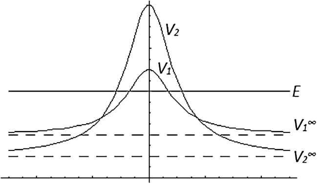
(H4): $\{\begin{matrix} There are only two crossing points in the domain Γ, y_{0}^{\pm} \in R . \\ E > V_{i} (y_{0}^{\pm}) . \\ There are only 4 turning points in Γ, x_{1}^{\pm} \in R for V_{1} - E and x_{2}^{\pm} \in R for V_{2} - E . \\ y_{0}^{-} < x_{2}^{-} < x_{1}^{-} < x_{1}^{+} < x_{2}^{+} < y_{0}^{+} . \\ At crossing points, we have: V_{1}^{'} (y_{0}^{\pm}) \neq V_{2}^{'} (y_{0}^{\pm}) \end{matrix}$

As example of potentials satisfying our hypotheses we take

V_{1} (x) = \frac{3}{x^{2} + 1} + 2, V_{2} (x) = \frac{7}{x^{2} + 1} + 1

and

E = 4

, see Figure 1.

Fig. 1.

Potentials.

2. Jost solutions

By analogy with the usual argument for the scalar Schrödinger operator, see [18], Theorem XI.57, the authors in [3] studied the behavior, at infinity, of the solutions of the system $P U = E U$ . Taking into account the assumption (H2), it was proven the existence of the so called Jost solutions.

Proposition 2.1.
Consider the free hamiltonian $P_{0} = - h^{2} \frac{d^{2}}{d x^{2}} I_{2} + V_{\infty}$ . Let $U_{0}$ be a solution of the free differential system $P_{0} U = E U$ . There exist two solutions $U^{d}$ and $U^{g}$ of the problem $P U = E U$ satisfying $\begin{matrix} \{\begin{matrix} {lim}_{x \to + \infty} U^{d} (x) - U_{0} (x) = 0, \\ {lim}_{x \to + \infty} {(U^{d})}^{'} (x) - U_{0}^{'} (x) = 0 \end{matrix} and \{\begin{matrix} {lim}_{x \to - \infty} U^{g} (x) - U_{0} (x) = 0, \\ {lim}_{x \to - \infty} {(U^{g})}^{'} (x) - U_{0}^{'} (x) = 0 . \end{matrix} \end{matrix}$
Definition 2.2.
Let $k_{j} = \sqrt{E - V_{j}^{\infty}}, j = 1, 2$ . We define and we denote by:
$U_{1 \pm}^{g}$ and $U_{2 \pm}^{g}$ the solutions given by Proposition 2.1 corresponding respectively to $U_{0 \pm} = (\begin{matrix} e^{\pm i k_{1} x / h} \\ 0 \end{matrix})$ and $U_{0 \pm} = (\begin{matrix} 0 \\ e^{\pm i k_{2} x / h} \end{matrix})$ in a neighborhood of $- \infty$ .

$U_{1 \pm}^{d}$ and $U_{2 \pm}^{d}$ the solutions given by Proposition 2.1 corresponding respectively to $U_{0 \pm} = (\begin{matrix} e^{\pm i k_{1} x / h} \\ 0 \end{matrix})$ and $U_{0 \pm} = (\begin{matrix} 0 \\ e^{\pm i k_{2} x / h} \end{matrix})$ in a neighborhood of $+ \infty$ .
The $U_{1 +}^{d}, U_{2 +}^{d}, U_{1 -}^{g} and U_{2 -}^{g}$ are called outgoing Jost solutions while the others are called incoming Jost solutions. We denote by M the matrix relating the outgoing solutions to the incoming ones (see Proposition A.3).

Let $S : = S (E) = {(s_{i j})}_{1 ⩽ i, j ⩽ 4}$ denote the scattering matrix associated with P and $P_{0}$ (see Definition A.1). The coefficients of S are related to those of the matrix M via the formulaes in Proposition A.3. The next objective is to compute the semiclassical behavior of the matrix M. To this end, we need to connect the left Jost solutions $U_{i \pm}^{g}$ and the right ones $U_{i \pm}^{d}$ . For this, we shall construct some transition solutions of the differential system $P U = E U$ . We begin with the construction of formal asymptotic solutions.
3. Formal solutions

3.1. Construction of formal solutions

In order to construct formal solutions near the turning points, we shall use the solutions of the Airy equation $\begin{matrix} (3.1) & ω^{″} - x ω = 0 . \end{matrix}$ Let us recall briefly some useful results (see for example [6,15]). There exists a unique solution $w_{1}$ of (3.1) having the asymptotic expansion as x tends to $- \infty$ $\begin{matrix} w_{1} (x) \sim {(- x)}^{- \frac{1}{4}} e^{i \frac{2}{3} {(- x)}^{\frac{3}{2}}} \sum_{n ⩾ 0} {(i)}^{n} α_{n} {(- x)}^{- \frac{3 n}{2}}, (x \mapsto - \infty) \end{matrix}$ with $α_{0} = 1$ and $\forall n ⩾ 0$ , $α_{n} \in R$ . Moreover, $\begin{matrix} w_{1}^{'} (x) \sim - i {(- x)}^{\frac{1}{4}} e^{i \frac{2}{3} {(- x)}^{\frac{3}{2}}} \sum_{n ⩾ 0} {(i)}^{n} β_{n} {(- x)}^{- \frac{3 n}{2}}, (x \mapsto - \infty), \end{matrix}$ with $β_{0} = 1$ and $\forall n ⩾ 0$ , $β_{n} \in R$ .

Also, recall that near $+ \infty$ , up to multiplication by a constant, there exists a unique exponential increasing solution $\begin{matrix} u (x) = \frac{1}{\sqrt{2}} (e^{i \frac{π}{4}} w_{1} + e^{- i \frac{π}{4}} {\overline{w}}_{1}) . \end{matrix}$ Observe that u is real and that the following expansions hold. $\begin{array}{l} u (x) \sim \sqrt{2} {(x)}^{- \frac{1}{4}} e^{\frac{2}{3} {(x)}^{\frac{3}{2}}} \sum_{n ⩾ 0} {(- 1)}^{n} α_{n} {(x)}^{- \frac{3 n}{2}}, (x \to + \infty) \\ u^{'} (x) \sim \sqrt{2} {(x)}^{\frac{1}{4}} e^{\frac{2}{3} {(x)}^{\frac{3}{2}}} \sum_{n ⩾ 0} {(- 1)}^{n} β_{n} {(x)}^{- \frac{3 n}{2}}, (x \to + \infty) . \end{array}$ A second real solution of the Airy equation (3.1) is given by $\begin{matrix} v = \frac{1}{\sqrt{2}} (e^{- i \frac{π}{4}} w_{1} + e^{i \frac{π}{4}} {\overline{w}}_{1}) . \end{matrix}$ For large positive x we get $\begin{array}{l} v (x) \sim \frac{1}{\sqrt{2}} {(x)}^{- \frac{1}{4}} e^{- \frac{2}{3} {(x)}^{\frac{3}{2}}} \sum_{n ⩾ 0} α_{n} {(x)}^{- \frac{3 n}{2}}, (x \to + \infty) \\ v^{'} (x) \sim - \frac{1}{\sqrt{2}} {(x)}^{\frac{1}{4}} e^{- \frac{2}{3} {(x)}^{\frac{3}{2}}} \sum_{n ⩾ 0} β_{n} {(x)}^{- \frac{3 n}{2}}, (x \to + \infty) . \end{array}$ Clearly, the wronskians $W (u, v) = 2$ and $W (ω_{1}, {\overline{ω}}_{1}) = - 2 i$ . We have $\begin{matrix} (3.2) & (\begin{matrix} v \\ u \end{matrix}) = T (\begin{matrix} ω_{1} \\ {\overline{ω}}_{1} \end{matrix}), T = \frac{1}{\sqrt{2}} (\begin{matrix} e^{- \frac{i π}{4}} & e^{\frac{i π}{4}} \\ e^{\frac{i π}{4}} & e^{- \frac{i π}{4}} \end{matrix}) . \end{matrix}$

Next, following [5] and [19], we construct, near each turning point, formal solutions of the system $\begin{matrix} (3.3) & P (x, h D_{x}, h) G (x, h, E) = E G (x, h, E) . \end{matrix}$ Consider ω a solution of the Airy equation. We shall construct solutions, associated with ω, as follows. $\begin{matrix} (3.4) & G (x, h, E) = (\begin{matrix} G_{1} (x, h, E) \\ G_{2} (x, h, E) \end{matrix}) \end{matrix}$ with $\begin{matrix} \{\begin{matrix} G_{1} (x, h, E) = h^{- \frac{1}{6}} A (x) ω (h^{- \frac{2}{3}} ξ (x)) + h^{\frac{1}{6}} B (x) ω^{'} (h^{- \frac{2}{3}} ξ (x)) \\ and \\ G_{2} (x, h, E) = h^{- \frac{1}{6}} C (x) ω (h^{- \frac{2}{3}} ξ (x)) + h^{\frac{1}{6}} D (x) ω^{'} (h^{- \frac{2}{3}} ξ (x)), \end{matrix} \end{matrix}$ where $\begin{matrix} A (x) = \sum_{n ⩾ 0} h^{n} A_{n}, B (x) = \sum_{n ⩾ 0} h^{n} B_{n}, C (x) = \sum_{n ⩾ 0} h^{n} C_{n} and D (x) = \sum_{n ⩾ 0} h^{n} D_{n} . \end{matrix}$

Substituting (3.4) in (3.3) yields $\begin{matrix} \{\begin{matrix} (1) : - h^{2} \frac{d^{2}}{d x^{2}} G_{1} (x, h, E) + (V_{1} (x) - E) G_{1} (x, h, E) + h R (x, h D_{x}) G_{2} (x, h, E) = 0, \\ (2) : - h^{2} \frac{d^{2}}{d x^{2}} G_{2} (x, h, E) + (V_{2} (x) - E) G_{2} (x, h, E) + h R (x, h D_{x}) G_{1} (x, h, E) = 0 . \end{matrix} \end{matrix}$ By annihilating the coefficients of ω and $ω^{'}$ one gets $\begin{array}{l} \{\begin{matrix} (I) : h^{2} (A^{″} + i c_{1} C^{'}) + h (2 B^{'} ξ ξ^{'} + B ξ ξ^{″} + B {(ξ^{'})}^{2} - c_{0} C + i c_{1} D ξ ξ^{'}) \\ + A ({(ξ^{'})}^{2} ξ - (V_{1} - E)) = 0 \\ (II) : h^{2} (B^{″} + i c_{1} D^{'}) + h (2 A^{'} ξ^{'} + A ξ^{″} - c_{0} D + i c_{1} C ξ^{'}) + B ({(ξ^{'})}^{2} ξ - (V_{1} - E)) = 0 . \end{matrix} \\ \{\begin{matrix} (III) : h^{2} (C^{″} + i c_{1} A^{'}) + h (2 D^{'} ξ ξ^{'} + D ξ ξ^{″} + D {(ξ^{'})}^{2} - c_{0} A + i c_{1} B ξ ξ^{'}) \\ + C ({(ξ^{'})}^{2} ξ - (V_{2} - E)) = 0 \\ (IV) : h^{2} (D^{″} + i c_{1} B^{'}) + h (2 C^{'} ξ^{'} + C ξ^{″} - c_{0} B + i c_{1} A ξ^{'}) + D ({(ξ^{'})}^{2} ξ - (V_{2} - E)) = 0 . \end{matrix} \end{array}$ Annihilating the leading terms in $(I)$ and $(III)$ yields two eiconal equations, $\begin{array}{l} (3.5) & {(ξ^{'} (x))}^{2} ξ (x) = (V_{1} (x) - E), \\ (3.6) & {(ξ^{'} (x))}^{2} ξ (x) = (V_{2} (x) - E) . \end{array}$ First, we construct formal solutions associated to the eiconal equation (3.5). This construction is valid inside $I_{1}^{-} =] x_{1}^{-} - η, x_{1}^{-} + η [$ and $I_{1}^{+} =] x_{1}^{+} - η, x_{1}^{+} + η [$ , with $η > 0$ small enough to assure that the second corresponding turning point $x_{1}^{+}$ respectively $x_{1}^{-}$ , as well as the crossing points $y_{0}^{\pm}$ , lie outside this interval. The same construction is also valid in the left interval $I_{\infty}^{-} =] - \infty, y_{0}^{-} - η [$ , respectively in the right one $I_{\infty}^{+} =] y_{0}^{+} + η, + \infty [$ . We fix a determination of $\sqrt{V_{1} - E}$ and define the function $\begin{matrix} (3.7) & ξ (x) = {(\frac{3}{2} \int_{x_{1}^{\pm}}^{x} {(V_{1} (t) - E)}^{\frac{1}{2}} d t)}^{\frac{2}{3}} \end{matrix}$ that is a solution of (3.5) which is regular in $I_{1}^{\pm}$ .

Thus the equations $(III)$ and $(IV)$ imply necessarily that $C_{0} = D_{0} = 0$ .

The equation $(I)$ yields $2 B_{0}^{'} (x) ξ (x) ξ^{'} (x) + B_{0} (x) {(ξ (x) ξ^{'} (x))}^{'} = 0$ , which implies that $\begin{matrix} B_{0} (x) = δ_{0} {(ξ (x) ξ^{'} (x))}^{- \frac{1}{2}}, for some δ_{0} \in C . \end{matrix}$ Since $B_{0}$ should be continuous it follows that $δ_{0} = 0$ and hence $B_{0} = 0$ .

Likewise $(II)$ yields $2 A^{'} (x) ξ^{'} (x) + A (x) ξ^{″} (x) = 0$ and therefore $\begin{matrix} A_{0} (x) = γ_{0} {(ξ^{'} (x))}^{- \frac{1}{2}}, for some γ_{0} \in C . \end{matrix}$ It follows from (3.5) that $\begin{matrix} (3.8) & A_{0} (x) = γ_{0} {(V_{1} (x) - E)}^{- \frac{1}{4}} {(ξ (x))}^{\frac{1}{4}}, x \in I_{1}^{\pm} . \end{matrix}$

On the other hand $(III)$ implies that $- c_{0} A_{0} + C_{1} ({(ξ^{'})}^{2} ξ - (V_{2} - E)) = 0$ . Thus $\begin{matrix} C_{1} (x) = \frac{c_{0} γ_{0} {(ξ^{'} (x))}^{- \frac{1}{2}}}{V_{1} (x) - V_{2} (x)} . \end{matrix}$

The equation $(IV)$ yields $i c_{1} A_{0} ξ^{'} + D_{1} ({(ξ^{'})}^{2} ξ - (V_{2} - E)) = 0$ which implies that $\begin{matrix} D_{1} (x) = \frac{- i c_{1} γ_{0} {(ξ^{'} (x))}^{\frac{1}{2}}}{V_{1} (x) - V_{2} (x)} . \end{matrix}$ By annihilating the coefficient of $h^{2}$ , it follows from $(I)$ that $A_{0}^{″} + 2 B_{1}^{'} ξ ξ^{'} + B_{1} ξ ξ^{″} + B_{1} {(ξ^{'})}^{2} - c_{0} C_{1} + i c_{1} D_{1} ξ ξ^{'} = 0$ which gives $B_{1}$ .

Likewise, it follows from $(II)$ that $B_{0}^{″} + 2 A_{1}^{'} ξ^{'} + A_{1} ξ^{″} - c_{0} D_{1} + i c_{1} C_{1} ξ^{'} = 0$ , which gives $A_{1}$ .

By annihilating the coefficients of $h^{n + 1}$ in $(I), (II), (III)$ and $(IV)$ , we are led to the following system of equations. $\begin{array}{l} 2 B_{n}^{'} ξ ξ^{'} + B_{n} (ξ ξ^{″} + {(ξ^{'})}^{2}) = c_{0} C_{n} - i c_{1} D_{n} ξ ξ^{'} - (A_{n - 1}^{″} + i c_{1} C_{n - 1}^{'}) . \\ 2 A_{n}^{'} ξ^{'} + A_{n} ξ^{″} = c_{0} D_{n} - i c_{1} C_{n} ξ^{'} - (B_{n - 1}^{″} + i c_{1} D_{n - 1}^{'}) . \\ 2 D_{n}^{'} ξ ξ^{'} + D_{n} (ξ ξ^{″} + {(ξ^{'})}^{2}) = c_{0} A_{n} - i c_{1} B_{n} ξ ξ^{'} - (C_{n - 1}^{″} + i c_{1} A_{n - 1}^{'}) . \\ 2 C_{n}^{'} ξ^{'} + C_{n} ξ^{″} = c_{0} B_{n} - i c_{1} A_{n} ξ^{'} - (D_{n - 1}^{″} + i c_{1} B_{n - 1}^{'}) . \end{array}$

This inductive process gives successively $A_{n}, B_{n}, C_{n}$ and $D_{n}$ . Notice that the expressions of $A, B, C$ and D are actually independent of the considered Airy solution.

Analogous constructions yield formal solutions corresponding to the eiconal equation (3.6) that are valid inside the intervals $I_{2}^{\pm} =] x_{2}^{\pm} - η, x_{2}^{\pm} + η [$ and $I_{\infty}^{\pm}$ with $η > 0$ small enough.

3.2. Connection formulas for formal solutions

Consider the formal solutions of the equation (3.3) constructed as in the preceding section corresponding to the turning points $x_{i}^{\pm}, i = 1, 2$ $\begin{matrix} (3.9) & g_{x_{i}^{\pm}} = (\begin{matrix} g_{1 x_{i}^{\pm}} \\ g_{2 x_{i}^{\pm}} \end{matrix}), h_{x_{i}^{\pm}} = (\begin{matrix} h_{1 x_{i}^{\pm}} \\ h_{2 x_{i}^{\pm}} \end{matrix}), f_{x_{i}^{\pm}} = (\begin{matrix} f_{1 x_{i}^{\pm}} \\ f_{2 x_{i}^{\pm}} \end{matrix}), f_{x_{i}^{\pm}}^{*} = (\begin{matrix} f_{1 x_{i}^{\pm}}^{*} \\ f_{2 x_{i}^{\pm}}^{*} \end{matrix}) \end{matrix}$ associated respectively with the Airy solutions $u, v, w_{1}, {\overline{w}}_{1}$ .

It follows from (3.2) that $\begin{matrix} (3.10) & (\begin{matrix} h_{x_{i}^{+}} \\ g_{x_{i}^{+}} \end{matrix}) = \frac{1}{\sqrt{2}} (\begin{matrix} e^{- \frac{i π}{4}} & e^{\frac{i π}{4}} \\ e^{\frac{i π}{4}} & e^{- \frac{i π}{4}} \end{matrix}) (\begin{matrix} f_{x_{i}^{+}} \\ f_{x_{i}^{+}}^{*}, \end{matrix}) . \end{matrix}$

By taking into consideration the expansions of the Airy solutions at $\pm \infty$ , one gets $\begin{matrix} (3.11) & g_{x_{1}^{-}} = e^{\frac{1}{h} \int_{x_{1}^{-}}^{x} {(V_{1} - E)}^{\frac{1}{2}} d t} \sqrt{2} \sum_{n ⩾ 0} h^{n} \sum_{k + l = n} {(- 1)}^{l} ξ^{- \frac{3 l}{2}} (\begin{matrix} A_{k} ξ^{- \frac{1}{4}} α_{l} + B_{k} ξ^{\frac{1}{4}} β_{l} \\ C_{k} ξ^{- \frac{1}{4}} α_{l} + D_{k} ξ^{\frac{1}{4}} β_{l} \end{matrix}), \end{matrix}$ in a neighborhood of $x_{1}^{-}$ as $h \to 0$ and $\begin{matrix} (3.12) & h_{x_{1}^{+}} = e^{- \frac{1}{h} \int_{x_{1}^{+}}^{x} {(V_{1} - E)}^{\frac{1}{2}} d t} \frac{1}{\sqrt{2}} \sum_{n ⩾ 0} h^{n} \sum_{k + l = n} ξ^{- \frac{3 l}{2}} (\begin{matrix} E_{k} ξ^{- \frac{1}{4}} α_{l} - F_{k} ξ^{\frac{1}{4}} β_{l} \\ G_{k} ξ^{- \frac{1}{4}} α_{l} - H_{k} ξ^{\frac{1}{4}} β_{l} \end{matrix}), \end{matrix}$ in a neighborhood of $x_{1}^{+}$ as $h \to 0$ .

4. Exact solutions

In this section we construct exact solutions, with known asymptotic expansions on some fixed interval, of the problem $P U = E U$ that we can write $\begin{matrix} (4.1) & - h^{2} \frac{d^{2}}{d x^{2}} U + V_{E} U = 0, with V_{E} = (\begin{matrix} V_{1} (x) - E & h R (x, h D_{x}) \\ h R (x, h D_{x}) & V_{2} (x) - E \end{matrix}) . \end{matrix}$ First, observe that, for $k = 1, 2$ , $g_{x_{k}^{-}} = i z_{k} h_{x_{k}^{+}} (1 + O (h^{\infty}))$ and $h_{x_{k}^{-}} = i {(z_{k})}^{- 1} g_{x_{k}^{+}} (1 + O (h^{\infty}))$ , with $z_{k} = e^{\frac{S_{k}}{h}} (1 + O (h))$ and $S_{k} = \int_{x_{k}^{-}}^{x_{k}^{+}} {(V_{k} - E)}^{\frac{1}{2}} d t$ . Now, let $θ_{x_{k}^{-}} + θ_{x_{k}^{+}} = 1$ be a smooth unit partition, where, for some $ε > 0$ , $θ_{x_{k}^{-}} = 1 on] - \infty, x_{k}^{-} + ε [and θ_{x_{k}^{+}} = 1 on] x_{k}^{+} - ε, + \infty [$ .

Define the functions $\begin{matrix} r_{k} = g_{x_{k}^{-}} θ_{x_{k}^{-}} + i z_{k} h_{x_{k}^{+}} θ_{x_{k}^{+}} and s_{k} = i g_{x_{k}^{+}} θ_{x_{k}^{+}} + z_{k} h_{x_{k}^{-}} θ_{x_{k}^{-}} \end{matrix}$ which are formal solutions of the equation (4.1). Introduce the notations $\begin{matrix} ρ_{r_{k}} (x) : = | e^{\frac{1}{h} \int_{x_{k}^{-}}^{x} {(V_{k} (t) - E)}^{\frac{1}{2}} d t} | and ρ_{s_{k}} (x) : = | e^{- \frac{1}{h} \int_{x_{k}^{+}}^{x} {(V_{k} (t) - E)}^{\frac{1}{2}} d t} | . \end{matrix}$ It is clear that $\begin{matrix} ρ_{r_{k}} (x) ρ_{s_{k}} (x) = z_{0 k} : = e^{\frac{S_{k}}{h}} . \end{matrix}$

Consider the finite sums of the asymptotic expansions of $r_{k}, s_{k}$ and denote them $r_{k}^{N}, s_{k}^{N}$ . According to the definition of $r_{k}$ and $s_{k}$ , we have $\begin{matrix} | r_{k}^{N} | + | h {(r_{k}^{N})}^{'} | ⩽ C_{N} ρ_{r_{k}} and | s_{k}^{N} | + | h {(s_{k}^{N})}^{'} | ⩽ C_{N} ρ_{s_{k}} . \end{matrix}$ As usual, $| y |$ for a vector $y = (y_{1}, y_{2})$ means the $max (| y_{1} |, | y_{2} |)$ .

Let $z_{k}^{N}$ be the cut series of $z_{k}$ . A simple computation yields $\begin{matrix} (4.2) & W (r_{1}^{N}, s_{1}^{N}, r_{2}^{N}, s_{2}^{N}) = {(z_{1} z_{2})}^{N} + z_{01} z_{02} O (h^{N}) . \end{matrix}$ Introduce four new almost solutions. $\begin{matrix} Y_{k} = \frac{r_{k}^{N}}{{(W (r_{1}^{N}, s_{1}^{N}, r_{2}^{N}, r_{2}^{N}))}^{\frac{1}{4}}} and Y_{2 + k} = \frac{s_{k}^{N}}{{(W (r_{1}^{N}, s_{1}^{N}, r_{2}^{N}, r_{2}^{N}))}^{\frac{1}{4}}}, k = 1, 2 . \end{matrix}$ According to (4.2), we deduce that for $k = 1, 2$ , $\begin{matrix} (4.3) & | Y_{k} | + | h Y_{k}^{'} | ⩽ C_{N} {(z_{01} z_{02})}^{- \frac{1}{4}} ρ_{r_{k}} and | Y_{2 + k} | + | h Y_{2 + k}^{'} | ⩽ C_{N} {(z_{01} z_{02})}^{- \frac{1}{4}} ρ_{s_{k}} . \end{matrix}$ Since $W (Y_{1}, Y_{2}, Y_{3}, Y_{4}) = 1$ it follows that there exist analytic functions $a_{i j}, b_{i j}$ such that all of $Y_{1}, \dots, Y_{4}$ satisfy the system $\begin{matrix} - h^{2} \frac{d^{2}}{d x^{2}} Y + W_{E} Y = 0, where W_{E} = (\begin{matrix} a_{11} + b_{11} h \frac{d}{d x} & a_{12} + b_{12} h \frac{d}{d x} \\ a_{21} + b_{21} h \frac{d}{d x} & a_{22} + b_{22} h \frac{d}{d x} \end{matrix}) . \end{matrix}$ Now, we construct solutions of the differential system (4.1) in the form $\begin{matrix} (4.4) & ψ = (\begin{matrix} ψ_{1} \\ ψ_{2} \end{matrix}) : = Y (x) + \sum_{i = 1}^{4} (\int_{x_{0}}^{x} A_{i} ψ (t) d t) Y_{i} (x), \end{matrix}$ where $Y \in Span (Y_{1}, Y_{2}, Y_{3}, Y_{4})$ and for $i \in {1, \dots, 4}$ , $A_{i}$ is the differential operator given by $\begin{matrix} A_{i} ψ = α_{i} (t, h) ψ_{1} + β_{i} (t, h) ψ_{2} + γ_{i} (t, h) h \frac{d}{d t} ψ_{1} + δ_{i} (t, h) h \frac{d}{d t} ψ_{2}, \end{matrix}$ with $α_{i}, β_{i}, γ_{i}$ and $δ_{i}$ are analytic functions satisfying, for arbitrary ψ, $\begin{matrix} (4.5) & \{\begin{matrix} \sum_{i = 1}^{4} A_{i} ψ (x) Y_{i} (x) = 0, \\ h^{2} \sum_{i = 1}^{4} A_{i} ψ (x) Y_{i}^{'} (x) = (V_{E} - W_{E}) ψ (x) . \end{matrix} \end{matrix}$ The existence of the analytic functions follows since $W (Y_{1}, \dots, Y_{4}) = 1$ . One can easily see that if we take ψ in the form (4.4), then by using (4.5) it follows that ψ is a solution of the differential system (4.1). Let K be the matrix operator given by $\begin{matrix} K (x, t) = (\begin{matrix} \sum_{i = 1}^{4} y_{i 1} (x) (α_{i} (t) + γ_{i} (t) \frac{d}{d t}) & \sum_{i = 1}^{4} y_{i 1} (x) (β_{i} (t) + δ_{i} (t) \frac{d}{d t}) \\ \sum_{i = 1}^{4} y_{i 2} (x) (α_{i} (t) + γ_{i} (t) \frac{d}{d t}) & \sum_{i = 1}^{4} y_{i 2} (x) (β_{i} (t) + δ_{i} (t) \frac{d}{d t}) \end{matrix}) . \end{matrix}$ The equation (4.4) writes $\begin{matrix} (4.6) & ψ (x) = Y (x) + \int_{x_{0}}^{x} K (x, t) ψ (t) d t, \end{matrix}$ where $x_{0}$ is some fixed point and $Y \in Span (Y_{1}, \dots, Y_{4})$ . The solution of the integral equation (4.6) satisfies the differential equation (4.1), its initial data in $x_{0}$ coincide with the initial data of Y. Now, we construct the exact solution $ψ_{r_{k}}$ , $k = 1, 2$ . We define the sequence of functions $\begin{matrix} \{\begin{matrix} ψ_{r_{k}}^{0} = Y_{k}, \\ ψ_{r_{k}}^{n + 1} = Y_{k} + \int_{x_{k}^{-}}^{x} K (x, t) ψ_{r_{k}}^{n} (t) d t . \end{matrix} \end{matrix}$ By taking into account that the coefficients of the differential matrix $V_{E} - W_{E}$ are $O (h^{N})$ we deduce from (4.3) and (4.5) that $\begin{matrix} max (| α_{i} |, | β_{i} |, | γ_{i} |, | δ_{i} |) ⩽ \{\begin{matrix} C_{N} h^{N} {(z_{01} z_{02})}^{\frac{1}{4}} ρ_{r_{i}}^{- 1}, & if i = 1, 2, \\ C_{N} h^{N} {(z_{01} z_{02})}^{\frac{1}{4}} ρ_{s_{i}}^{- 1}, & if i = 3, 4 . \end{matrix} \end{matrix}$ It follows that $\begin{matrix} | ψ_{r_{k}}^{1} - ψ_{r_{k}}^{0} | = | \int_{x_{k}^{-}}^{x} K (x, t) Y_{k} (t) d t | ⩽ C_{N} h^{N} {(z_{01} z_{02})}^{- \frac{1}{4}} ρ_{r_{k}} (x) (x - x_{k}^{-}) . \end{matrix}$ It is easily shown by induction that $\begin{matrix} | ψ_{r_{k}}^{m} - ψ_{r_{k}}^{m - 1} | ⩽ C_{N} {(z_{01} z_{02})}^{- \frac{1}{4}} ρ_{r_{k}} (x) \frac{{(h^{N} (x - x_{k}^{-}))}^{m}}{m!}, \end{matrix}$ which implies that the sequence $(ψ_{r_{k}}^{m})$ converges uniformly for $x \in [y_{0}^{-} + 2 ε, y_{0}^{+} - 2 ε]$ and $0 < h < h_{0}$ . The limit function $ψ_{r_{k}}$ satisfies the integral equation (4.6). Furthermore, we have $\begin{matrix} \forall x \in [y_{0}^{-} + 2 ε, y_{0}^{+} - 2 ε], | ψ_{r_{k}}^{m} (x) - Y_{k} (x) | ⩽ \sum_{0 ⩽ l ⩽ m - 1} | ψ_{r_{k}}^{l + 1} (x) - ψ_{r_{k}}^{l} (x) | . \end{matrix}$ It follows that $\begin{matrix} | ψ_{r_{k}} (x) - Y_{k} (x) | ⩽ D_{N} {(z_{01} z_{02})}^{- \frac{1}{4}} ρ_{r_{k}} (x) h^{N}, \end{matrix}$ with $D_{N} = C_{N} (x - x_{k}^{-}) e^{O (h^{N})}$ . Hence, $ψ_{r_{k}}$ has the same asymptotic development as $Y_{k}$ up to the order $N - 1$ on $[y_{0}^{-} + 2 ε, y_{0}^{+} - 2 ε]$ . It is clear that on $[y_{0}^{-} + 2 ε, y_{0}^{+} - 2 ε]$ $\begin{matrix} ψ_{r_{k}} = {(z_{1}^{N} z_{2}^{N})}^{- \frac{1}{4}} r_{k}^{N - 1} + {(z_{01} z_{02})}^{- \frac{1}{4}} ρ_{r_{k}} (x) O (h^{N}) . \end{matrix}$ With the same method, we construct the exact solutions $ψ_{s_{k}}$ so that $\begin{matrix} ψ_{s_{k}} = {(z_{1}^{N} z_{2}^{N})}^{- \frac{1}{4}} s_{k}^{N - 1} + {(z_{01} z_{02})}^{- \frac{1}{4}} ρ_{s_{k}} (x) O (h^{N}) . \end{matrix}$ Moreover, $\begin{matrix} W (ψ_{r_{1}}, ψ_{s_{1}}, ψ_{r_{2}}, ψ_{s_{2}}) = 1 + O (h^{N}) . \end{matrix}$

We have constructed on the interval $(y_{0}^{-}, y_{0}^{+})$ four solutions $ψ_{r_{k}}$ and $ψ_{s_{k}}$ , $k = 1, 2$ , with a known asymptotic behavior and with a known Wronskian. As a result, on finite vicinities of the turning points, we have four linearly independent solutions with a known asymptotic behavior. Introduce now, on these vicinities, sets of canonical solutions. Consider on a vicinity of $x_{k}^{-}$ two solutions $\begin{matrix} {\tilde{v}}_{k g}^{-} = \frac{{(z_{1}^{N} z_{2}^{N})}^{\frac{1}{4}}}{z_{k}^{N}} ψ_{s_{k}} and {\tilde{v}}_{k g}^{+} = {(z_{1}^{N} z_{2}^{N})}^{\frac{1}{4}} ψ_{r_{k}} . \end{matrix}$ We have $W ({\tilde{v}}_{1 g}^{+}, {\tilde{v}}_{1 g}^{-}, {\tilde{v}}_{2 g}^{+}, {\tilde{v}}_{2 g}^{-}) = W (ψ_{r_{1}}, ψ_{s_{1}}, ψ_{r_{2}}, ψ_{s_{2}}) = 1 + O (h^{N})$ . Let us normalize these solutions $\begin{matrix} v_{k g}^{\pm} = {(W ({\tilde{v}}_{1 g}^{+}, {\tilde{v}}_{1 g}^{-}, {\tilde{v}}_{2 g}^{+}, {\tilde{v}}_{2 g}^{-}))}^{- \frac{1}{4}} {\tilde{v}}_{k g}^{\pm} . \end{matrix}$ Notice that

∙ ${(v_{k g}^{+})}^{N} = {(g_{x_{k}^{-}})}^{N} and {(v_{k g}^{-})}^{N} = {(h_{x_{k}^{-}})}^{N} on] x_{k}^{-}, x_{k}^{+} [$ .

Considering the formal solutions $r_{k} = f_{x_{k}^{-}} and s_{k} = f_{x_{k}^{-}}^{*}$ , on $] y_{0}^{-}, x_{k}^{-} [$ and then on $] - \infty, y_{0}^{-} [$ leads to analogous constructions of exact solutions $u_{k g}^{+}$ and $u_{k g}^{-}$ and then $w_{k g}^{+}$ and $w_{k g}^{-}$ , with

∙ ${(u_{k g}^{+})}^{N} = {(f_{x_{k}^{-}})}^{N}, {(u_{k g}^{-})}^{N} = {(f_{x_{k}^{-}}^{*})}^{N} on] y_{0}^{-}, x_{k}^{-} [$ .

∙ ${(w_{k g}^{+})}^{N} = {(f_{x_{k}^{-}})}^{N}, {(w_{k g}^{-})}^{N} = {(f_{x_{k}^{-}}^{*})}^{N} on] - \infty, y_{0}^{-} [$ .

Analogous constructions provide exact solutions $v_{k d}^{\pm}, u_{k d}^{\pm}$ and $w_{k d}^{\pm}$ on the right hand side so that

∙ ${(v_{k d}^{+})}^{N} = {(g_{x_{k}^{+}})}^{N}, {(v_{k d}^{-})}^{N} = {(h_{x_{k}^{+}})}^{N} on] x_{k}^{-}, x_{k}^{+} [$ ,

∙ ${(u_{k d}^{+})}^{N} = {(f_{x_{k}^{+}})}^{N}, {(u_{k d}^{-})}^{N} = {(f_{x_{k}^{+}}^{*})}^{N} on] x_{k}^{+}, y_{0}^{+} [$ ,

∙ ${(w_{k d}^{+})}^{N} = {(f_{x_{k}^{+}})}^{N}, {(w_{k d}^{-})}^{N} = {(f_{x_{k}^{+}}^{*})}^{N} on] y_{0}^{+}, + \infty [$ .

The asymptotic formulae (3.11) and (3.12), and also the analogous asymptotic expansions for $f_{x_{i}^{\pm}}$ , $f_{x_{i}^{\pm}}^{*}$ , $h_{x_{i}^{\pm}}$ and $g_{x_{i}^{\pm}}$ lead to the following theorem.

Theorem 4.1.
Let $ϵ > 0$ be small enough, the following expansions hold as h tends to 0.
$w_{1 g}^{\pm} = e^{\mp \frac{1}{h} \int_{x_{1}^{-}}^{x} {(V_{1} (t) - E)}^{\frac{1}{2}} d t} [(\begin{matrix} {(E - V_{1})}^{- \frac{1}{4}} \\ 0 \end{matrix}) + O (h)]$ , on $] - \infty, y_{0}^{-} - ϵ [$ .

$w_{2 g}^{\pm} = e^{\mp \frac{1}{h} \int_{x_{2}^{-}}^{x} {(V_{2} - E)}^{\frac{1}{2}} d t} [(\begin{matrix} 0 \\ {(E - V_{2})}^{- \frac{1}{4}} \end{matrix}) + O (h)]$ , on $] - \infty, y_{0}^{-} - ϵ [$ .

$u_{1 g}^{\pm} = e^{\mp \frac{1}{h} \int_{x_{1}^{-}}^{x} {(V_{1} (t) - E)}^{\frac{1}{2}} d t} [(\begin{matrix} {(E - V_{1})}^{- \frac{1}{4}} \\ 0 \end{matrix}) + O (h)]$ , on $] y_{0}^{-} + ϵ, x_{1}^{-} - ϵ [$ .

$u_{2 g}^{\pm} = e^{\mp \frac{1}{h} \int_{x_{2}^{-}}^{x} {(V_{2} - E)}^{\frac{1}{2}} d t} [(\begin{matrix} 0 \\ {(E - V_{2})}^{- \frac{1}{4}} \end{matrix}) + O (h)]$ , on $] y_{0}^{-} + ϵ, x_{2}^{-} - ϵ [$ .

$v_{1 g}^{\pm} = {(\frac{1}{\sqrt{2}})}^{\mp 1} e^{\pm \frac{1}{h} \int_{x_{1}^{-}}^{x} {(V_{1} - E)}^{\frac{1}{2}} d t} [(\begin{matrix} {(V_{1} - E)}^{- \frac{1}{4}} \\ 0 \end{matrix}) + O (h)]$ , on $] x_{1}^{-} + ϵ, x_{1}^{+} - ϵ [$ .

$v_{2 g}^{\pm} = {(\frac{1}{\sqrt{2}})}^{\mp 1} e^{\pm \frac{1}{h} \int_{x_{2}^{-}}^{x} {(V_{2} - E)}^{\frac{1}{2}} d t} [(\begin{matrix} 0 \\ {(V_{2} - E)}^{- \frac{1}{4}} \end{matrix}) + O (h)]$ , on $] x_{2}^{-} + ϵ, x_{2}^{+} - ϵ [$ .

$w_{1 d}^{\pm} = {(- 1)}^{- \frac{1}{2}} e^{\pm \frac{1}{h} \int_{x_{1}^{+}}^{x} {(V_{1} - E)}^{\frac{1}{2}} d t} [(\begin{matrix} {(E - V_{1})}^{- \frac{1}{4}} \\ 0 \end{matrix}) + O (h)]$ , on $] y_{0}^{+} + ϵ, + \infty [$ .

$w_{2 d}^{\pm} = {(- 1)}^{- \frac{1}{2}} e^{\pm \frac{1}{h} \int_{x_{2}^{+}}^{x} {(V_{2} - E)}^{\frac{1}{2}} d t} [(\begin{matrix} 0 \\ {(E - V_{2})}^{- \frac{1}{4}} \end{matrix}) + O (h)]$ , on $] y_{0}^{+} + ϵ, + \infty [$ .

$u_{1 d}^{\pm} = {(- 1)}^{- \frac{1}{2}} e^{\pm \frac{1}{h} \int_{x_{1}^{+}}^{x} {(V_{1} - E)}^{\frac{1}{2}} d t} [(\begin{matrix} {(E - V_{1})}^{- \frac{1}{4}} \\ 0 \end{matrix}) + O (h)]$ , on $] x_{1}^{+} + ϵ, y_{0}^{+} - ϵ [$ .

$u_{2 d}^{\pm} = {(- 1)}^{- \frac{1}{2}} e^{\pm \frac{1}{h} \int_{x_{2}^{+}}^{x} {(V_{2} - E)}^{\frac{1}{2}} d t} [(\begin{matrix} 0 \\ {(E - V_{2})}^{- \frac{1}{4}} \end{matrix}) + O (h)]$ , on $] x_{2}^{+} + ϵ, y_{0}^{+} - ϵ [$ .

$v_{1 d}^{\pm} = {(\frac{1}{\sqrt{2}})}^{\pm 1} {(- 1)}^{- \frac{1}{2}} e^{\pm \frac{1}{h} \int_{x_{1}^{+}}^{x} {(V_{1} - E)}^{\frac{1}{2}} d t} [(\begin{matrix} {(V_{1} - E)}^{- \frac{1}{4}} \\ 0 \end{matrix}) + O (h)]$ , on $] x_{1}^{-} + ϵ, x_{1}^{+} - ϵ [$ .

$v_{2 d}^{\pm} = {(\frac{1}{\sqrt{2}})}^{\pm 1} {(- 1)}^{- \frac{1}{2}} e^{\pm \frac{1}{h} \int_{x_{2}^{+}}^{x} {(V_{2} - E)}^{\frac{1}{2}} d t} [(\begin{matrix} 0 \\ {(V_{2} - E)}^{- \frac{1}{4}} \end{matrix}) + O (h)]$ , on $] x_{2}^{-} + ϵ, x_{2}^{+} - ϵ [$ .

5. Transition matrices

Observe that $B_{+} = (w_{1 d}^{+}, w_{1 g}^{-}, w_{2 d}^{+}, w_{2 g}^{-})$ and $B_{-} = (w_{1 g}^{+}, w_{1 d}^{-}, w_{2 g}^{+}, w_{2 d}^{-})$ are two fundamental systems of solutions of the differential system $P U = E U$ . We consider $T = {(t_{i j})}_{1 ⩽ i, j ⩽ 4}$ the interaction matrix defined by $\begin{matrix} (\begin{matrix} w_{1 d}^{+} \\ w_{1 g}^{-} \\ w_{2 d}^{+} \\ u_{2 g}^{-} \end{matrix}) = T (\begin{matrix} w_{1 g}^{+} \\ w_{1 d}^{-} \\ w_{2 g}^{+} \\ w_{2 d}^{-} \end{matrix}) . \end{matrix}$

5.1. Connection at infinity

In this section, we shall connect the Jost solutions $U_{i \pm}^{d}$ and $U_{i \pm}^{g}$ to the systems of solutions $B_{+}$ and $B_{-}$ . The first step toward this is to introduce the right and the left actions $S_{d_{j}}$ and $S_{g_{j}}, j = 1, 2$ . $\begin{array}{l} S_{d_{j}} = - k_{j} x_{j}^{+} + \int_{x_{j}^{+}}^{+ \infty} {(E - V_{j} (x))}^{\frac{1}{2}} - k_{j} d x, \\ S_{g_{j}} = - k_{j} x_{j}^{-} - \int_{- \infty}^{x_{j}^{-}} {(E - V_{j} (x))}^{\frac{1}{2}} - k_{j} d x, \end{array}$ where $k_{j} = \sqrt{E - V_{j}^{\infty}}$ . Thanks to the assumption (H2), these quantities are well defined. Next, we compare the asymptotic expansions of $w_{j g}^{\pm}$ and $w_{j d}^{\pm}$ with $U_{j \pm}^{d}$ et $U_{j \pm}^{g}$ . Following [7], Appendice B, we get:

Proposition 5.1.
$\begin{matrix} (\begin{matrix} U_{1 \pm}^{d} \\ U_{1 \pm}^{g} \\ U_{2 \pm}^{d} \\ U_{2 \pm}^{g} \end{matrix}) = (\begin{matrix} r_{1 \pm}^{d} & 0 & 0 & 0 \\ 0 & r_{1 \pm}^{g} & 0 & 0 \\ 0 & 0 & r_{2 \pm}^{d} & 0 \\ 0 & 0 & 0 & r_{2 \pm}^{g} \end{matrix}) (\begin{matrix} w_{1 d}^{\pm} \\ w_{1 g}^{\pm} \\ w_{2 d}^{\pm} \\ w_{2 g}^{\pm} \end{matrix}) \end{matrix}$

with $r_{j \pm}^{d} = i k_{j}^{\frac{1}{2}} e^{\mp i \frac{S_{d_{j}}}{h}} (1 + O (h))$ , and $r_{j \pm}^{g} = k_{j}^{\frac{1}{2}} e^{\mp i \frac{S_{g_{j}}}{h}} (1 + O (h)), j = 1, 2$ .

According to Proposition A.3 together with Proposition 5.1, we get the following result. Lemma 5.2.
Let $S = {(s_{i j})}_{1 ⩽ i, j ⩽ 4}$ be the scattering matrix. Then $\begin{array}{l} {\bar{s}}_{11} = \frac{r_{1 +}^{d}}{r_{1 +}^{g}} t_{11}, {\bar{s}}_{12} = - \frac{r_{1 +}^{d}}{r_{1 -}^{d}} t_{12}, {\bar{s}}_{13} = \frac{r_{1 +}^{d}}{r_{2 +}^{g}} \sqrt{\frac{k_{2}}{k_{1}}} t_{13}, {\bar{s}}_{14} = - \frac{r_{1 +}^{d}}{r_{2 -}^{d}} \sqrt{\frac{k_{2}}{k_{1}}} t_{14}, \\ {\bar{s}}_{21} = - \frac{r_{1 -}^{g}}{r_{1 +}^{g}} t_{21}, {\bar{s}}_{22} = \frac{r_{1 -}^{g}}{r_{1 -}^{d}} t_{22}, {\bar{s}}_{23} = - \frac{r_{1 -}^{g}}{r_{2 +}^{g}} \sqrt{\frac{k_{2}}{k_{1}}} t_{23}, {\bar{s}}_{24} = \frac{r_{1 -}^{g}}{r_{2 -}^{d}} \sqrt{\frac{k_{2}}{k_{1}}} t_{24}, \\ {\bar{s}}_{31} = \frac{r_{2 +}^{d}}{r_{1 +}^{g}} \sqrt{\frac{k_{1}}{k_{2}}} t_{31}, {\bar{s}}_{32} = - \frac{r_{2 +}^{d}}{r_{1 -}^{d}} \sqrt{\frac{k_{1}}{k_{2}}} t_{32}, {\bar{s}}_{33} = \frac{r_{2 +}^{d}}{r_{2 +}^{g}} t_{33}, s_{34} = - \frac{r_{2 +}^{d}}{r_{2 -}^{d}} t_{34}, \\ {\bar{s}}_{41} = - \frac{r_{2 -}^{g}}{r_{1 +}^{g}} \sqrt{\frac{k_{1}}{k_{2}}} t_{41}, {\bar{s}}_{42} = \frac{r_{2 -}^{g}}{r_{1 -}^{d}} \sqrt{\frac{k_{1}}{k_{2}}} t_{42}, {\bar{s}}_{43} = - \frac{r_{2 -}^{g}}{r_{2 +}^{g}} t_{43}, {\bar{s}}_{44} = \frac{r_{2 -}^{g}}{r_{2 -}^{d}} t_{44} . \end{array}$

5.2. Connection near the turning points

Equation (3.10) and Theorem 4.1 yield the following proposition.

Proposition 5.3.
Consider $M_{g}$ , $M_{c}$ and $M_{d}$ the transition matrices defined by $\begin{matrix} (\begin{matrix} v_{1 g}^{-} \\ v_{1 g}^{+} \\ v_{2 g}^{-} \\ v_{2 g}^{+} \end{matrix}) = M_{g} (\begin{matrix} u_{1 g}^{+} \\ u_{1 g}^{-} \\ u_{2 g}^{+} \\ u_{2 g}^{-} \end{matrix}), (\begin{matrix} v_{1 d}^{+} \\ v_{1 d}^{-} \\ v_{2 d}^{+} \\ v_{2 d}^{-} \end{matrix}) = M_{c} (\begin{matrix} v_{1 g}^{-} \\ v_{1 g}^{+} \\ v_{2 g}^{-} \\ v_{2 g}^{+} \end{matrix}) and (\begin{matrix} v_{1 d}^{+} \\ v_{1 d}^{-} \\ v_{2 d}^{+} \\ v_{2 d}^{-} \end{matrix}) = M_{d} (\begin{matrix} u_{1 d}^{+} \\ u_{1 d}^{-} \\ u_{2 d}^{+} \\ u_{2 d}^{-} \end{matrix}) . \end{matrix}$ Then, $\begin{matrix} M_{g} = M_{d} = \frac{1}{\sqrt{2}} (\begin{matrix} e^{- i \frac{π}{4}} & e^{i \frac{π}{4}} & 0 & 0 \\ e^{i \frac{π}{4}} & e^{- i \frac{π}{4}} & 0 & 0 \\ 0 & 0 & e^{- i \frac{π}{4}} & e^{i \frac{π}{4}} \\ 0 & 0 & e^{i \frac{π}{4}} & e^{- i \frac{π}{4}} \end{matrix}) and M_{c} = (\begin{matrix} 0 & - i z_{1}^{- 1} & 0 & 0 \\ - i z_{1} & 0 & 0 & 0 \\ 0 & 0 & 0 & - i z_{2}^{- 1} \\ 0 & 0 & - i z_{2} & 0 \end{matrix}) \end{matrix}$ where $z_{i} = 2 e^{\frac{S_{i}}{h}} (1 + O (h))$ with $S_{i} = \int_{x_{i}^{-}}^{x_{i}^{+}} {(V_{i} (t) - E)}^{\frac{1}{2}} d t, i = 1, 2$ .
Proposition 5.4.
$\begin{matrix} (\begin{matrix} u_{1 d}^{+} \\ u_{1 g}^{+} \\ u_{2 d}^{+} \\ u_{2 g}^{+} \end{matrix}) = T_{c} (\begin{matrix} u_{1 g}^{-} \\ u_{1 d}^{-} \\ u_{2 g}^{-} \\ u_{2 d}^{-} \end{matrix}), with T_{c} = (\begin{matrix} \frac{- 2 i z_{1}}{1 + z_{1}^{2}} & - i \frac{- 1 + z_{1}^{2}}{1 + z_{1}^{2}} & 0 & 0 \\ - i \frac{- 1 + z_{1}^{2}}{1 + z_{1}^{2}} & \frac{2 i z_{1}}{1 + z_{1}^{2}} & 0 & 0 \\ 0 & 0 & \frac{- 2 i z_{2}}{1 + z_{2}^{2}} & - i \frac{- 1 + z_{2}^{2}}{1 + z_{2}^{2}} \\ 0 & 0 & - i \frac{- 1 + z_{2}^{2}}{1 + z_{2}^{2}} & \frac{2 i z_{2}}{1 + z_{2}^{2}} \end{matrix}) . \end{matrix}$
Proof.
The $(u_{d})$ are expressed in terms of the $(u_{g})$ as follows $\begin{matrix} (\begin{matrix} u_{1 d}^{+} \\ u_{1 d}^{-} \\ u_{2 d}^{+} \\ u_{2 d}^{-} \end{matrix}) = M_{d}^{- 1} M_{c} M_{g} (\begin{matrix} u_{1 g}^{+} \\ u_{1 g}^{-} \\ u_{2 g}^{+} \\ u_{2 g}^{+} \end{matrix}) . \end{matrix}$ It follows from Proposition 5.3 that $\begin{matrix} M_{d}^{- 1} M_{c} M_{g} = - \frac{1}{2} (\begin{matrix} - z_{1}^{- 1} + z_{1} & i (z_{1}^{- 1} + z_{1}) & 0 & 0 \\ i (z_{1}^{- 1} + z_{1}) & z_{1}^{- 1} - z_{1} & 0 & 0 \\ 0 & 0 & - z_{2}^{- 1} + z_{2}) & i (z_{2}^{- 1} + z_{2}) \\ 0 & 0 & i (z_{2}^{- 1} + z_{2}) & z_{2}^{- 1} - z_{2} \end{matrix}) \end{matrix}$ whence the result follows easily. □

6. Microlocal reduction

In order to describe the asymptotic expansion of the coefficients of the scattering matrix, we need to determine the matrix M (see Proposition A.3). In view of Proposition 5.4 and Lemma 5.2, all that remains to do is to connect the $(w_{i d})$ to the $(u_{i d})$ on the right, and the $(w_{i g})$ to the $(u_{i g})$ on the left. Notice that by symmetry, the computation on one side is analogous to that on the other side. For the sake of simplicity we shall assume that the $V_{i}$ and the $c_{i}$ are even functions. However, we are going to try not to lose the generality in the final results.

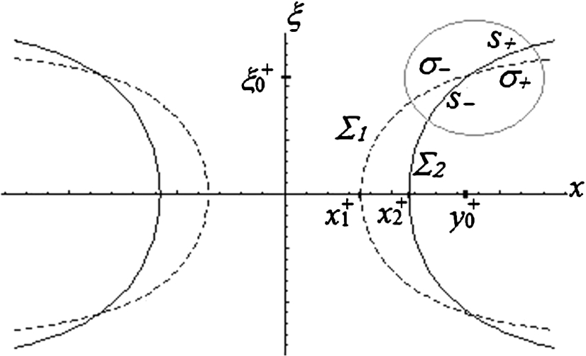
First, we develop a microlocal analysis on the operator P near the crossing points. Recall that the real characteristic manifold of $P - E$ , is the union of two components $Σ_{1}$ and $Σ_{2}$ that cross at the real points $(y_{0}^{+}, \pm ξ_{0}^{+})$ and $(y_{0}^{-}, \pm ξ_{0}^{-})$ with $V_{1} (y_{0}^{\pm}) = V_{2} (y_{0}^{\pm})$ and $ξ_{0}^{\pm} = \sqrt{E - V_{i} (y_{0}^{\pm})}$ . We make an ellipticity assumption on the coupling term $R (x, h D_{x})$ near the crossing points $(y_{0}^{+}, ξ_{0}^{\pm})$ .

(H5): $c_{1}^{2} (y_{0}^{\pm}) (E - V_{1} (y_{0}^{\pm})) - c_{0}^{2} (y_{0}^{\pm}) \neq 0$ .

Under the condition (H5), the operator R has a microlocal inverse $R^{- 1}$ near the point $(y_{0}^{+}, ξ_{0}^{+})$ . Writing the system $(P - E) U = 0$ as follows $\begin{matrix} (6.1) & \{\begin{matrix} (P_{1} - E) u_{1} + h R u_{2} = 0, \\ (P_{2} - E) u_{2} + h R u_{1} = 0, \end{matrix} \end{matrix}$ the second equation yields (microlocally near the point $(y_{0}^{+}, ξ_{0}^{+})$ ) $\begin{matrix} (6.2) & h u_{1} = - R^{- 1} (P_{2} - E) u_{2} . \end{matrix}$ Substituting this into the first equation of (6.1), we obtain $\begin{matrix} ((P_{1} - E) R^{- 1} (P_{2} - E) - h^{2} R) u_{2} = 0 . \end{matrix}$ Observe that the operator $Q : = R (P_{1} - E) R^{- 1} (P_{2} - E) - h^{2} R^{2}$ has a real principal symbol having a saddle point at $(y_{0}^{+}, ξ_{0}^{+})$ which is non-degenerate since $V_{1}^{'} (y_{0}^{+}) \neq V_{2}^{'} (y_{0}^{+})$ . Applying the microlocal reduction theorem ([11], Theorem b1) reduces the study of the operator Q near $(y_{0}^{+}, ξ_{0}^{+})$ to that of $p_{0} = \frac{1}{2} (x h D_{x} + h D_{x} x)$ near the point $(0, 0)$ . More precisely, one obtains the following proposition.

Proposition 6.1.
Under the hypotheses (H1), (H4), (H5), there exist a classical analytic symbol of order two $μ_{h}^{+}$ and a unitary formal Fourier integral operator H related to a canonical transformation κ defined near $(0, 0)$ with $κ (0, 0) = (y_{0}^{+}, ξ_{0}^{+})$ such that the following equivalence holds.

A microlocal distribution $u_{0} (\cdot, h)$ defined in a neighborhood of $(0, 0)$ is a solution of the model equation $p_{0} u_{0} = (- \frac{i}{2} h + μ_{h}^{+}) u_{0}$ if and only if $U = (\begin{matrix} - R^{- 1} (P_{2} - E) H u_{0} \\ h H u_{0} \end{matrix})$ is a microlocal solution near $(y_{0}^{+}, ξ_{0}^{+})$ of the system $(P - E) U = 0$ .
Proof.
For simplicity we shall use x for $x - y_{0}^{+}$ and ξ for $ξ - ξ_{0}^{+}$ . Then the principal symbol of Q writes $q_{0} (x, ξ) = 4 {(ξ_{0}^{+})}^{2} (ξ + τ_{1} x) (ξ + τ_{2} x) + O ({(x, ξ)}^{3})$ near $(0, 0)$ , with $τ_{i} = \frac{V_{i}^{'} (y_{0}^{+})}{2 ξ_{0}^{+}}$ . Observe that by (H4), $τ_{2} < τ_{1} < 0$ . By [11], Theorem b1 there is a unitary Fourier integral operator H, with canonical transformation κ defined near $(0, 0)$ with $κ (0, 0) = (0, 0)$ , and a classical analytic symbol $F (t, h)$ of order 0 such that $\begin{matrix} (6.3) & H^{} F (Q, h) H = p_{0} . \end{matrix}$ One can write formally $\begin{matrix} H u (x) = \frac{1}{\sqrt{2 π h}} \int e^{i ψ (x, y) / h} a (x, y, h) u (y) d y, \end{matrix}$ with $\begin{matrix} ψ (x, y) = - \frac{τ_{1}}{2} x^{2} + \sqrt{τ_{1} - τ_{2}} x y - \frac{1}{2} y^{2} + O ({(x, y)}^{3}) . \end{matrix}$ The canonical transformation κ is defined near $(0, 0)$ by $\begin{matrix} κ (y, - \partial_{y} ψ (x, y)) = (x, \partial_{x} ψ (x, y)) . \end{matrix}$ One gets $κ (y, η) = (x, ξ)$ with $\begin{matrix} (ξ + τ_{1} x, ξ + τ_{2} x) = (\sqrt{τ_{1} - τ_{2}} y, \sqrt{τ_{1} - τ_{2}} η) + O ({(y, η)}^{2}) . \end{matrix}$ By (6.3) the equation $Q H u = 0$ is microlocally, in a neigborhood of $(0, 0)$ , equivalent to the equation $\begin{matrix} p_{0} u = F (0, h) u . \end{matrix}$ Writing $F (t, h) = f_{0} (t) + h f_{1} (t) + \dots$ yields $f_{0} (q_{0} \circ κ (x, ξ)) = x ξ$ , which in turn implies that $f_{0} (0) = 0$ and further that $\begin{matrix} (6.4) & f_{0}^{'} (0) = \frac{1}{4 {(ξ_{0}^{+})}^{2} (τ_{1} - τ_{2})} . \end{matrix}$ Using the functional calculus developed in [11], Appendix a, we see that the Weyl symbol of $H^{} F (Q, h) H$ is $F (q \circ κ (x, ξ), h) + O (h^{2})$ , where $q = q_{0} + h q_{1} + \dots$ denotes the Weyl symbol of Q. It follows from (6.3) that $\begin{matrix} f_{0}^{'} (0) q_{1} (0, 0) + f_{1} (0) = 0 . \end{matrix}$ On the other hand by writing $Q = (P_{1} - E) (P_{2} - E) + [R, P_{1} - E] R^{- 1} (P_{2} - E) - h^{2} R^{2}$ we see that $\begin{matrix} q_{1} (0, 0) = 2 i {(ξ_{0}^{+})}^{2} (τ_{1} - τ_{2}) . \end{matrix}$ Then $f_{1} (0) = - \frac{i}{2}$ and therefore $\begin{matrix} (6.5) & F (0, h) = - \frac{i}{2} h + μ_{h}^{+}, \end{matrix}$ where $μ_{h}^{+}$ is a classical analytic symbol of order two. The proposition follows from (6.2). □

In the following lemma we compute the principal symbol of $μ_{h}^{+}$ . Lemma 6.2.
$\begin{matrix} μ_{h}^{+} = {(μ^{+} h)}^{2} + O (h^{3}), with μ^{+} = \frac{c_{0} (y_{0}^{+}) + c_{1} (y_{0}^{+}) ξ_{0}^{+}}{2 ξ_{0}^{+} \sqrt{τ_{1} - τ_{2}}} . \end{matrix}$
Proof.
Let ω be a function defined near $y_{0}^{+}$ solution of $(P_{2} - E) ω = 0$ satisfying the initial conditions $ω (y_{0}^{+}) = 1$ and $h D_{x} ω (y_{0}^{+}) = ξ_{0}^{+}$ . The existence of ω is well known, see [17], Proposition 2, for the construction of such solution. It follows immediately that $\begin{matrix} (6.6) & Q ω = - h^{2} R^{2} ω . \end{matrix}$ Now, we move to the point $(0, 0)$ by using a translation. According to (6.3) we get $\begin{matrix} H^{} F (Q, h) = (x h D_{x} - i \frac{h}{2}) H^{} . \end{matrix}$ Writing $F (t, h) = F (0, h) + F_{1} (t, h) t$ yields $\begin{matrix} (6.7) & (x h D_{x} - i \frac{h}{2}) H^{} ω = F (0, h) H^{} ω - h^{2} H^{} F_{1} (Q, h) R^{2} ω . \end{matrix}$ This identity is valid microlocally near $(0, 0)$ . By applying a FBI transform and then taking $x = 0$ we get $\begin{matrix} (6.8) & (F (0, h) + i \frac{h}{2}) H^{} ω (0) = h^{2} (H^{} F_{1} (Q, h) R^{2} ω) (0) . \end{matrix}$ Now, write $F_{1} (t, h) = F_{1}^{0} (t) + O (h)$ , then by (6.4) $\begin{matrix} F_{1}^{0} (0) = \frac{1}{4 {(ξ_{0}^{+})}^{2} (τ_{1} - τ_{2})} . \end{matrix}$ By using the fact that operators commute up to an $O (h)$ factor, it follows that $\begin{matrix} F_{1} (Q, h) R^{2} = R^{2} F_{1}^{0} (Q) + O (h) . \end{matrix}$ In combination with (6.6) the last equation yields $\begin{matrix} F_{1} (Q, h) R^{2} ω = R^{2} F_{1}^{0} (0) ω + O (h) . \end{matrix}$ Thus $\begin{matrix} H^{} F_{1} (Q, h) R^{2} ω = F_{1}^{0} (0) R^{2} H^{} ω + O (h) . \end{matrix}$ It follows from (6.8) that $\begin{matrix} (F (0, h) + i \frac{h}{2}) (H^{} ω) (0) = h^{2} F_{1}^{0} (0) (R^{2} H^{} ω) (0) + O (h^{3}) . \end{matrix}$ On the other hand combining (6.5) with (6.7) gives, near $(0, 0)$ , $\begin{matrix} H^{} ω = c + O (h) \end{matrix}$ with c a constant which is non null since ω is not and H is unitary. By moving back to $(y_{0}^{+}, ξ_{0}^{+})$ we get easily $\begin{matrix} F (0, h) = - i \frac{h}{2} + h^{2} F_{1}^{0} (0) {(c_{0} (y_{0}^{+}) + c_{1} (y_{0}^{+}) ξ_{0}^{+})}^{2} + O (h^{3}) . \end{matrix}$ □

6.1. Solutions of the model equation

Consider the differential equation arising in the above proposition. $\begin{matrix} (6.9) & p_{0} u = (- \frac{i}{2} h + μ_{h}^{+}) u . \end{matrix}$ Let Y denotes the Heaviside function. A fundamental system of solutions of the equation (6.9) in the space of microlocal distributions defined near $(0, 0)$ is provided by $\begin{matrix} u_{\pm} (x, h, μ_{h}^{+}) = | x |^{i \frac{μ_{h}^{+}}{h}} Y (\pm x) . \end{matrix}$ Let $J$ denotes the operator of complex conjugation and $F_{h}$ denotes the semi-classical Fourier transform. It’s easy to observe that $p_{0}$ and $F_{h}^{- 1} J$ are commuting. Using this fact yields a second fundamental system of solutions of (6.9) given by $\begin{matrix} u_{\pm}^{*} (x, h, μ_{h}^{+}) = F_{h}^{- 1} (u_{\pm} (\cdot, h, i h - μ_{h}^{+})) (x) . \end{matrix}$ Define $B_{μ_{h}^{+}}$ the interaction matrix connecting the system $(u_{+}, u_{-})$ to $(u_{+}^{*}, u_{-}^{*})$ in the following way. If $p u_{+} + q u_{-} = r u_{+}^{*} + s u_{-}^{*}$ , then $(p, q) = (r, s) B_{μ_{h}^{+}}$ . To compute this matrix we follow [10]. Let λ be a complex and consider $x_{\pm}^{λ} = | x |^{λ} Y (\pm x)$ . These distributions exist for $Re λ > - 1$ and extend analytically in $C ∖ {- 1, - 2, \dots}$ (see [10], Chapter 1, Section 3.2). Now, consider the distributions ${(x + i 0)}^{λ}$ which are analytic in the hole complex plane. From ([10], Chapter 1, Section 3.6) we have, for $Re λ > - 1$ , $\begin{matrix} (6.10) & \begin{matrix} {(x + i 0)}^{λ} = x_{+}^{λ} + e^{i λ π} x_{-}^{λ}, \\ {(x - i 0)}^{λ} = x_{+}^{λ} + e^{- i λ π} x_{-}^{λ} . \end{matrix} \end{matrix}$ These formulas remain true, by analytic continuation, for $λ \in C ∖ {- 1, - 2, \dots}$ . Also, from ([10], Chapter 2, Section 2.3), we have $\begin{matrix} (6.11) & \begin{matrix} F_{h}^{- 1} (\frac{x_{+}^{λ}}{Γ (λ + 1)}) = \frac{h^{λ + 1}}{\sqrt{2 π h}} e^{i (λ + 1) π / 2} {(x + i 0)}^{- λ - 1}, \\ F_{h}^{- 1} (\frac{x_{-}^{λ}}{Γ (λ + 1)}) = \frac{h^{λ + 1}}{\sqrt{2 π h}} e^{- i (λ + 1) π / 2} {(x - i 0)}^{- λ - 1}, \end{matrix} \end{matrix}$ where Γ denotes the Gamma function.

Since $μ_{h}^{+} / h$ is non zero and it is small, for small h, it follows by applying the formulas (6.11) for $λ = - 1 - i μ_{h}^{+} / h$ and then (6.10) for $λ = i μ_{h}^{+} / h$ that $\begin{matrix} B_{μ_{h}^{+}} = h^{- 1} N (μ_{h}^{+}, h) (\begin{matrix} e^{μ_{h}^{+} π / 2 h} & e^{- μ_{h}^{+} π / 2 h} \\ e^{- μ_{h}^{+} π / 2 h} & e^{μ_{h}^{+} π / 2 h} \end{matrix}), with N (μ_{h}^{+}, h) = \frac{1}{\sqrt{2 π}} h^{\frac{1}{2} - i \frac{μ_{h}^{+}}{h}} Γ (- i \frac{μ_{h}^{+}}{h}) . \end{matrix}$ We shall need below some knowledge about the microsupport (for short MS) of the distributions $u_{\pm}$ and $u_{\pm}^{*}$ . We have the following lemma, see [16], Proposition 8.1.

Lemma 6.3.
$MS (u_{\pm}) = {(y, ξ) \in R^{2} such that (\pm y > 0 and ξ = 0) or (y = 0)}$ and $MS (u_{\pm}^{*}) = {(y, ξ) \in R^{2} such that (\pm ξ > 0 and y = 0) or (ξ = 0)}$ .

6.2. Microlocal solutions

In view of Proposition 6.1, we get four microlocal solutions of the equation $(P - E) U = 0$ , namely $U_{\pm} = (\begin{matrix} u_{1, \pm} \\ u_{2, \pm} \end{matrix}) and U_{\pm}^{*} = (\begin{matrix} u_{1, \pm}^{*} \\ u_{2, \pm}^{*} \end{matrix})$ , where $\begin{array}{l} (6.12) & u_{2, \pm} = h H u_{\pm}, u_{2, \pm}^{*} = h H u_{\pm}^{*}, \\ u_{1, \pm} = - R^{- 1} (P_{2} - E) H u_{\pm} and u_{1, \pm}^{*} = - R^{- 1} (P_{2} - E) H u_{\pm}^{*} \end{array}$

We adopt the following notations, see Figure 2. $\begin{array}{l} σ_{\pm} = {(x, η) \in B ((y_{0}^{+}, ξ_{0}^{+}), ϵ) such that η^{2} + V_{1} (x) - E = 0 and \pm (x - y_{0}^{+}) > 0}, \\ s_{\pm} = {(x, η) \in B ((y_{0}^{+}, ξ_{0}^{+}), ϵ) such that η^{2} + V_{2} (x) - E = 0 and \pm (η - ξ_{0}^{+}) > 0} . \end{array}$

Fig. 2.

Characteristic manifold.

Combining Lemma 6.3 with (6.12) immediately yields the following result.

Proposition 6.4.

The microsupports of the solutions defined microlocally in the ball $B ((0, 0), ϵ)$ are included respectively in the closure of $\begin{array}{l} s_{+} \cup s_{-} \cup σ_{\pm} for U_{\pm}^{*}, \\ σ_{+} \cup σ_{-} \cup s_{\pm} for U_{\pm} . \end{array}$

6.3. Connection near the crossing points

In order to connect the solutions $U_{\pm}$ and $U_{\pm}^{*}$ to the $u_{i d}^{\pm}$ and $w_{i d}^{\pm}$ we need to analyze these distributions close to the microsupport. First, notice that along this text we choose the principal branch of the square root, that is positive on $R^{+}$ . Following [13], Section 4, we show that for $\frac{ϵ}{2} < (x - y_{0}^{+}) < ϵ$ , with $ϵ > 0$ small, the contribution of $u_{2, +} = h H u_{+}$ on $s_{+}$ is obtained by a stationary phase expansion. More precisely, write $\begin{array}{l} H u_{+} (x) & = \frac{1}{\sqrt{2 π h}} \int_{0}^{+ \infty} e^{i ψ (x, y) / h} a (x, y, h) | y |^{i μ_{h}^{+} / h} d y \\ = \frac{1}{\sqrt{2 π h}} \int_{0}^{+ \infty} e^{i ψ (x, y) / h} \tilde{a} (x, y, h) d y, \end{array}$ where, $\tilde{a} (x, y, h) = a_{0} (x, y) + h {\tilde{a}}_{1} (x, y) + \dots$ , with $a_{0} (0, 0) = 1$ , and $\begin{matrix} ψ (x, y) = - \frac{τ_{1}}{2} x^{2} + \sqrt{τ_{1} - τ_{2}} x y - \frac{1}{2} y^{2} + O ({(x, y)}^{3}) . \end{matrix}$ Note that we use here the reduced coordinates $(x, ξ)$ in place of $(x - y_{0}^{+}, ξ - ξ_{0}^{+})$ . Observe that $ψ (x, y)$ has one critical point $y_{c} (x)$ with respect to y, satisfying $y_{c} (0) = 0$ . By the stationary phase expansion one gets, at the level of principal symbols and microlocally near $s_{+}$ $\begin{matrix} u_{2, +} = h e^{- i \frac{π}{4}} a_{0} (x, y_{c} (x)) \frac{1}{\sqrt{| \partial_{y}^{2} ψ (x, y_{c} (x)) |}} e^{i ψ (x, y_{c} (x)) / h}, for \frac{ϵ}{2} < x < ϵ . \end{matrix}$ Back to the initial coordinates and define $\begin{matrix} Z_{k} (x, y_{0}^{+}) = \int_{y_{0}^{+}}^{x} {(E - V_{k} (t))}^{\frac{1}{2}} d t, k = 1, 2, \end{matrix}$ then $\begin{matrix} (6.13) & u_{2, +} (x, h) = e^{i Z_{2} (x, y_{0}^{+}) / h} h e^{- i \frac{π}{4}} a_{+} (x, h) microlocally on s_{+} . \end{matrix}$ where $a_{+}$ is an analytic symbol of order 0 defined near the interval $] y_{0}^{+} + \frac{ϵ}{2}, y_{0}^{+} + ϵ [$ with principal symbol $a_{+ 0} (x) = 1 + O (x - y_{0}^{+})$ .

Now observe that $H F_{h}^{- 1}$ is also a unitary Fourier integral operator that we can write formally $\begin{matrix} H F_{h}^{- 1} u (x) = \frac{e^{- i \frac{π}{4}}}{\sqrt{2 π h}} \int e^{i φ (x, y) / h} α (x, y, h) u (y) d y, \end{matrix}$ where $α (x, y, h) = α_{0} (x, y) + h α_{1} (x, y) + \dots$ , with $α_{0} (0, 0) = a_{0} (0, 0) = 1$ , and $\begin{matrix} φ (x, y) = - \frac{τ_{2}}{2} x^{2} + \sqrt{τ_{1} - τ_{2}} x y + \frac{1}{2} y^{2} + O ({(x, y)}^{3}) . \end{matrix}$ By arguing as above, we get the microlocal value of $u_{2, +}^{*} = h H F_{h}^{- 1} (u_{\pm} (\cdot, i h - μ_{h}^{+}))$ near $σ_{+}$ . $\begin{matrix} (6.14) & u_{2, +}^{*} (x, h) = e^{i Z_{1} (x, y_{0}^{+}) / h} \frac{h}{\sqrt{τ_{1} - τ_{2}} (x - y_{0}^{+})} a_{+}^{*} (x, h) microlocally on σ_{+}, \end{matrix}$ where $a_{+}^{*}$ is an analytic symbol of order 0 defined near the interval $] y_{0}^{+} + \frac{ϵ}{2}, y_{0}^{+} + ϵ [$ with principal symbol $a_{+ 0}^{*} (x) = 1 + O (x - y_{0}^{+})$ .

Now, we need to know the microlocal value of $u_{1, +}^{*} = - \frac{1}{h} R^{- 1} (P_{2} - E) u_{2, +}^{*}$ near $σ_{+}$ . Observe that at the level of principal symbols and microlocally near $σ_{+}$ we have $\begin{matrix} (P_{2} - E) u_{2, +}^{*} = (V_{2} - V_{1}) u_{2, +}^{*} . \end{matrix}$ By applying $- \frac{1}{h} R^{- 1}$ on the last equation, it follows from (6.14) that $\begin{matrix} (6.15) & u_{1, +}^{*} (x, h) = e^{i Z_{1} (x, y_{0}^{+}) / h} \frac{2 ξ_{0} \sqrt{τ_{1} - τ_{2}}}{c_{0} (y_{0}^{+}) + c_{1} (y_{0}^{+}) ξ_{0}^{+}} b_{+}^{*} (x, h) microlocally on σ_{+}, \end{matrix}$ where $b_{+}^{*}$ is an analytic symbol of order 0 defined near the interval $] y_{0}^{+} + \frac{ϵ}{2}, y_{0}^{+} + ϵ [$ with principal symbol $b_{+ 0}^{*} (x) = 1 + O (x - y_{0}^{+})$ .

Similarly, there exist two analytic symbols $a_{-}$ and $b_{-}^{*}$ , of order 0 defined near the real interval $] y_{0}^{+} - ϵ, y_{0}^{+} - \frac{ϵ}{2} [$ , with principal symbols $1 + O (x - y_{0}^{+})$ such that $\begin{matrix} (6.16) & \{\begin{matrix} u_{2, -} (x, h) = e^{i Z_{2} (x, y_{0}^{+}) / h} h e^{- i \frac{π}{4}} a_{-} (x, h) & on s_{-}, \\ u_{1, -}^{*} (x, h) = e^{i Z_{1} (x, y_{0}^{+}) / h} \frac{2 ξ_{0} \sqrt{τ_{1} - τ_{2}}}{c_{0} (y_{0}^{+}) + c_{1} (y_{0}^{+}) ξ_{0}^{+}} b_{-}^{*} (x, h) & on σ_{-} \end{matrix} \end{matrix}$ Let $ϕ_{j} = - Z_{j} (x_{j}^{+}, y_{0}^{+}) = \int_{x_{j}^{+}}^{y_{0}^{+}} {(E - V_{j} (t))}^{\frac{1}{2}} d t$ , $j = 1, 2$ . By normalizing the solutions $u_{i d}^{\pm}$ at $x_{i}^{+}$ it follows from the expansions (6.16) together with Theorem 4.1 that $\begin{matrix} (6.17) & \{\begin{matrix} u_{1 d}^{+} = a_{1}^{+} (h) e^{i ϕ_{1} / h} U_{-}^{*} & on σ_{-}, \\ h u_{2 d}^{+} = a_{2}^{+} (h) e^{i ϕ_{2} / h} U_{-} & on s_{-} \end{matrix} \end{matrix}$ where $a_{1}^{+}, a_{2}^{+}$ are two classical analytic symbols of order 0 with principal symbols $\begin{matrix} \{\begin{matrix} a_{1, 0}^{+} = - i μ^{+} {(E - V_{1} (y_{0}^{+}))}^{- \frac{1}{4}}, \\ a_{2, 0}^{+} = e^{- i \frac{π}{4}} {(E - V_{2} (y_{0}^{+}))}^{- \frac{1}{4}} \end{matrix} \end{matrix}$ Recall that the $w_{i d}^{\pm}$ are normalized at $y_{0}^{+}$ . By observing that $w_{2 d}^{+}$ has no microsupport on $σ_{+}$ and that $w_{1 d}^{+}$ has no microsupport on $s_{+}$ it follows from (6.13, 6.15) that $\begin{matrix} (6.18) & \{\begin{matrix} w_{1 d}^{+} = b_{1}^{+} (h) e^{i ϕ_{1} / h} U_{+}^{*} & on σ_{+}, \\ h w_{2 d}^{+} = b_{2}^{+} (h) e^{i ϕ_{2} / h} U_{+} & on s_{+} \end{matrix} \end{matrix}$ where $b_{1}^{+}$ and $b_{2}^{+}$ are two classical analytic symbols of order 0, with principal symbols $\begin{matrix} b_{i, 0}^{+} = a_{i, 0}^{+}, i = 1, 2 . \end{matrix}$

By using the interaction matrix $B_{μ_{h}^{+}}$ in combination with (6.12), we get $\begin{array}{l} U_{+} = \frac{1}{N (μ_{h}^{+}, h)} e^{\frac{μ_{h}^{+} π}{2 h}} h U_{-}^{*} - e^{\frac{μ_{h}^{+} π}{h}} U_{-} \\ h U_{+}^{*} = e^{\frac{μ_{h}^{+} π}{h}} h U_{-}^{*} + N (μ_{h}^{+}, h) (e^{- \frac{μ_{h}^{+} π}{2 h}} - e^{\frac{3 μ_{h}^{+} π}{2 h}}) U_{-} . \end{array}$ Thus, by taking into account that $e^{\pm μ_{h}^{+} π / h}$ is a classical analytic symbol of order 0 and principal symbol 1, we infer from (6.17), (6.18) the following results.

Proposition 6.5.
There exist classical analytic symbols $f_{i}^{+}$ and $g_{i}^{+}$ of order 0 each having principal symbol 1 such that
$w_{1 d}^{+} = f_{1}^{+} (h) u_{1 d}^{+} - \frac{2 π μ_{h}^{+}}{h} N (μ_{h}^{+}, h) e^{- i \frac{π}{4}} μ^{+} f_{2}^{+} (h) e^{i ϕ / h} u_{2 d}^{+}$ ,

$w_{2 d}^{+} = \frac{1}{N (μ_{h}^{+}, h) e^{- i \frac{π}{4}} μ^{+}} g_{1}^{+} (h) e^{- i ϕ / h} u_{1 d}^{+} - g_{2}^{+} (h) u_{2 d}^{+}$ .
where $ϕ = ϕ_{1} - ϕ_{2} = \int_{x_{1}^{+}}^{y_{0}^{+}} {(E - V_{1} (t))}^{\frac{1}{2}} d t - \int_{x_{2}^{+}}^{y_{0}^{+}} {(E - V_{2} (t))}^{\frac{1}{2}} d t$ .

By a similar analysis near $(y_{0}^{+}, - ξ_{0}^{+})$ , we obtain the following proposition.
Proposition 6.6.
There exist classical analytic symbols $f_{i}^{-}$ and $g_{i}^{-}$ of order 0 each having principal symbol 1 such that
$w_{1 d}^{-} = f_{1}^{-} (h) u_{1 d}^{-} - \frac{2 π \overline{μ_{h}^{-}}}{h} \overline{N} (μ_{h}^{-}, h) e^{i \frac{π}{4}} μ^{-} f_{2}^{-} (h) e^{- i ϕ / h} u_{2 d}^{-}$ ,

$w_{2 d}^{-} = \frac{1}{\overline{N} (μ_{h}^{-}, h) e^{i \frac{π}{4}} μ^{-}} g_{1}^{-} (h) e^{i ϕ / h} u_{1 d}^{-} - g_{2}^{-} (h) u_{2 d}^{-}$ ,
where $μ_{h}^{-} = {(μ^{-} h)}^{2} + O (h^{3}), with μ^{-} = \frac{c_{0} (y_{0}^{+}) - c_{1} (y_{0}^{+}) ξ_{0}^{+}}{2 ξ_{0}^{+} \sqrt{τ_{1} - τ_{2}}}$ .

By taking into consideration the symmetry of the problem, analogous formula hold for $w_{i g}^{\pm}$ .
Proposition 6.7.
There exist classical analytic symbols ${\tilde{f}}_{i}^{\pm}$ and ${\tilde{g}}_{i}^{\pm}$ of order 0 each having principal symbol 1 such that $\begin{array}{l} w_{1 g}^{+} = {\tilde{f}}_{1}^{+} (h) u_{1 g}^{+} - \frac{2 π \overline{μ_{h}^{+}}}{h} \overline{N} (μ_{h}^{+}, h) e^{i \frac{π}{4}} μ^{+} {\tilde{f}}_{2}^{+} (h) e^{- i ϕ / h} u_{2 g}^{+} \\ w_{2 g}^{+} = \frac{1}{\overline{N} (μ_{h}^{+}, h) e^{i \frac{π}{4}} μ^{+}} {\tilde{g}}_{1}^{+} (h) e^{i ϕ / h} u_{1 g}^{+} - {\tilde{g}}_{2}^{+} (h) u_{2 g}^{+} \\ w_{1 g}^{-} = {\tilde{f}}_{1}^{-} (h) u_{1 g}^{-} - \frac{2 π μ_{h}^{-}}{h} N (μ_{h}^{-}, h) e^{- i \frac{π}{4}} μ^{-} {\tilde{f}}_{2}^{-} (h) e^{i ϕ / h} u_{2 g}^{-} \\ w_{2 g}^{-} = \frac{1}{N (μ_{h}^{-}, h) e^{- i \frac{π}{4}} μ^{-}} {\tilde{g}}_{1}^{-} (h) e^{- i ϕ / h} u_{1 g}^{-} - {\tilde{g}}_{2}^{-} (h) u_{2 g}^{-} . \end{array}$

We notice that if $u (\cdot, h)$ is a holomorphic solution of the problem $(P - E) u = 0$ then the functions given by $\bar{u} (\bar{x}, h)$ and $u (- x, h)$ are holomorphic solutions of a similar problem obtained from P by replacing the function $c_{1}$ by $- c_{1}$ . This observation confirms the results in the Propositions 6.7 and 6.6.

Now, let $M_{+}$ and $M_{-}$ denote the interaction matrices defined as follows. $\begin{matrix} (\begin{matrix} w_{1 d}^{+} \\ w_{1 g}^{-} \\ w_{2 d}^{+} \\ w_{2 g}^{-} \end{matrix}) = M_{+} (\begin{matrix} u_{1 d}^{+} \\ u_{1 g}^{-} \\ u_{2 d}^{+} \\ u_{2 g}^{-} \end{matrix}) and (\begin{matrix} w_{1 g}^{+} \\ w_{1 d}^{-} \\ w_{2 g}^{+} \\ w_{2 d}^{-} \end{matrix}) = M_{-} (\begin{matrix} u_{1 g}^{+} \\ u_{1 d}^{-} \\ u_{2 g}^{+} \\ u_{2 d}^{-} \end{matrix}) . \end{matrix}$ Then, it follows from Propositions 6.5 and 6.6 that, up to multiplying each term by $(1 + O (h))$ , $\begin{matrix} M_{+} = (\begin{matrix} 1 & 0 & - \frac{2 π μ_{h}^{+}}{h} N^{+} μ^{+} e^{- i \frac{π}{4}} e^{i \frac{ϕ}{h}} & 0 \\ 0 & 1 & 0 & - \frac{2 π μ_{h}^{-}}{h} N^{-} μ^{-} e^{- i \frac{π}{4}} e^{i \frac{ϕ}{h}} \\ \frac{e^{i \frac{π}{4}} e^{- i \frac{ϕ}{h}}}{N^{+} μ^{+}} & 0 & - 1 & 0 \\ 0 & \frac{e^{i \frac{π}{4}} e^{- i \frac{ϕ}{h}}}{N^{-} μ^{-}} & 0 & - 1 \end{matrix}) \end{matrix}$ where we use $N^{\pm}$ for $N (μ_{h}^{\pm}, h)$ . Also, up to multiplying each term by $(1 + O (h))$ , we can write $\begin{matrix} M_{-} = (\begin{matrix} 1 & 0 & - \frac{2 π \overline{μ_{h}^{+}}}{h} \overline{N^{+}} μ^{+} e^{i \frac{π}{4}} e^{- i \frac{ϕ}{h}} & 0 \\ 0 & 1 & 0 & - \frac{2 π \overline{μ_{h}^{-}}}{h} \overline{N^{-}} μ^{-} e^{i \frac{π}{4}} e^{- i \frac{ϕ}{h}} \\ \frac{e^{- i \frac{π}{4}} e^{i \frac{ϕ}{h}}}{\overline{N^{+}} μ^{+}} & 0 & - 1 & 0 \\ 0 & \frac{e^{- i \frac{π}{4}} e^{i \frac{ϕ}{h}}}{\overline{N^{-}} μ^{-}} & 0 & - 1 \end{matrix}) \end{matrix}$

Recall that $\begin{matrix} (\begin{matrix} w_{1 d}^{+} \\ w_{1 g}^{-} \\ w_{2 d}^{+} \\ w_{2 g}^{-} \end{matrix}) = T (\begin{matrix} w_{1 g}^{+} \\ w_{1 d}^{-} \\ w_{2 g}^{+} \\ w_{2 d}^{-} \end{matrix}) and (\begin{matrix} u_{1 d}^{+} \\ u_{1 g}^{-} \\ u_{2 d}^{+} \\ u_{2 g}^{-} \end{matrix}) = T_{c} (\begin{matrix} u_{1 g}^{+} \\ u_{1 d}^{-} \\ u_{2 g}^{+} \\ u_{2 d}^{-} \end{matrix}), \end{matrix}$ which implies that $T = M_{+} T_{c} M_{-}^{- 1}$ . Thus we get the following proposition.
Proposition 6.8.
Let $S_{1} = \int_{x_{1}^{-}}^{x_{1}^{+}} {(V_{1} (t) - E)}^{\frac{1}{2}} d t$ . Then, up to multiplication by $(1 + O (h))$ terms for $h > 0$ in a neighborhood of 0, we have $\begin{array}{l} t_{11} = - i e^{- \frac{S_{1}}{h}}, t_{12} = - i, \\ t_{21} = - i, t_{22} = i e^{- \frac{S_{1}}{h}}, \\ t_{33} = - \frac{2 π \overline{μ_{h}^{+}}}{h} e^{- \frac{S_{1}}{h}} e^{- 2 i ϕ / h} \frac{\overline{N^{+}}}{N^{+}}, t_{34} = - i, \\ t_{43} = - i, t_{44} = \frac{2 π \overline{μ_{h}^{-}}}{h} e^{- \frac{S_{1}}{h}} e^{- 2 i ϕ / h} \frac{\overline{N^{-}}}{N^{-}}, \\ t_{13} = - \frac{2 π \overline{μ_{h}^{+}}}{h} \overline{N^{+}} μ^{+} e^{- \frac{S_{1}}{h}} e^{- i \frac{π}{4}} e^{- i ϕ / h}, \\ t_{14} = - (\frac{2 π μ_{h}^{+}}{h} N^{+} μ^{+} e^{i \frac{π}{4}} e^{i ϕ / h} + \frac{2 π \overline{μ_{h}^{-}}}{h} \overline{N^{-}} μ^{-} e^{- i \frac{π}{4}} e^{- i ϕ / h}), \\ t_{24} = \frac{2 π \overline{μ_{h}^{-}}}{h} \overline{N^{-}} μ^{-} e^{- \frac{S_{1}}{h}} e^{- i \frac{π}{4}} e^{- i ϕ / h}, \\ t_{23} = - (\frac{2 π μ_{h}^{-}}{h} N^{-} μ^{-} e^{i \frac{π}{4}} e^{i ϕ / h} + \frac{2 π \overline{μ_{h}^{+}}}{h} \overline{N^{+}} μ^{+} e^{- i \frac{π}{4}} e^{- i ϕ / h}), \\ t_{31} = \frac{1}{N^{+} μ^{+}} e^{- \frac{S_{1}}{h}} e^{- i \frac{π}{4}} e^{- i ϕ / h}, t_{32} = (\frac{1}{\overline{N^{-}} μ^{-}} e^{i \frac{π}{4}} e^{i ϕ / h} + \frac{1}{N^{+} μ^{+}} e^{- i \frac{π}{4}} e^{- i ϕ / h}), \\ t_{42} = - \frac{1}{N^{-} μ^{-}} e^{- \frac{S_{1}}{h}} e^{- i \frac{π}{4}} e^{- i ϕ / h}, t_{41} = (\frac{1}{\overline{N^{+}} μ^{+}} e^{i \frac{π}{4}} e^{i ϕ / h} + \frac{1}{N^{-} μ^{-}} e^{- i \frac{π}{4}} e^{- i ϕ / h}) . \end{array}$

Recall that $μ_{h}^{\pm} = {(μ^{\pm} h)}^{2} + O (h^{3})$ is a classical symbol of order 2 which implies, see [15], Part 2, that $Γ (- i \frac{μ_{h}^{\pm}}{h}) = \frac{i}{{(μ^{\pm})}^{2} h} (1 + O (h))$ . Then $\begin{matrix} N^{\pm} = \frac{1}{\sqrt{2 π}} h^{\frac{1}{2} - i \frac{μ_{h}^{\pm}}{h}} Γ (- i \frac{μ_{h}^{\pm}}{h}) = \frac{i}{\sqrt{2 π h} {(μ^{\pm})}^{2}} (1 + O (h log h)) . \end{matrix}$ Hence $\begin{matrix} \frac{2 π μ_{h}^{\pm}}{h} N^{\pm} μ^{\pm} = \sqrt{2 π h} i μ^{\pm} (1 + O (h log h)), \end{matrix}$ while $\begin{matrix} \frac{1}{N^{\pm} μ^{\pm}} = - \sqrt{2 π h} i μ^{\pm} (1 + O (h log h)) . \end{matrix}$

According to Proposition 6.8 and by using Lemma 5.2, we get the following theorem.
Theorem 6.9 (Scattering matrix).

Assume (H1)–(H5). Then for $h > 0$ in a neighborhood of 0, we have:

The upper diagonal block $S_{11}$ : $\begin{array}{l} s_{11} = e^{- \frac{S_{1}}{h}} e^{i \frac{S_{d_{1}} - S_{g_{1}}}{h}} (1 + O (h)), s_{12} = i e^{2 i \frac{S_{d_{1}}}{h}} (1 + O (h)), \\ s_{21} = i e^{- 2 i \frac{S_{g_{1}}}{h}} (1 + O (h)), s_{22} = e^{- \frac{S_{1}}{h}} e^{i \frac{S_{d_{1}} - S_{g_{1}}}{h}} (1 + O (h)) . \end{array}$

The lower diagonal block $S_{22}$ : $\begin{array}{l} s_{33} = 2 i π {(μ^{+})}^{2} e^{- \frac{S_{1}}{h}} e^{i \frac{S_{d_{2}} - S_{g_{2}}}{h}} e^{2 i ϕ / h} h (1 + O (h)), s_{34} = i e^{2 i \frac{S_{d_{2}}}{h}} (1 + O (h)), \\ s_{44} = 2 i π {(μ^{-})}^{2} e^{- \frac{S_{1}}{h}} e^{i \frac{S_{d_{2}} - S_{g_{2}}}{h}} e^{2 i ϕ / h} h (1 + O (h)), s_{43} = i e^{- 2 i \frac{S_{g_{2}}}{h}} (1 + O (h) . \end{array}$

The upper off-diagonal block $S_{12}$ : $\begin{array}{l} s_{13} = - i e^{- \frac{S_{1}}{h}} e^{i \frac{S_{d_{1}} - S_{g_{2}}}{h}} e^{- i \frac{π}{4}} e^{i ϕ / h} μ^{+} \sqrt{2 π h} (1 + O (h log h)), \\ s_{14} = e^{i \frac{S_{d_{1}} + S_{d_{2}}}{h}} (e^{i \frac{π}{4}} e^{- i ϕ / h} μ^{+} + e^{- i \frac{π}{4}} e^{i ϕ / h} μ^{-}) \sqrt{2 π h} (1 + O (h log h)), \\ s_{23} = e^{- i \frac{S_{g_{1}} + S_{g_{2}}}{h}} (e^{i \frac{π}{4}} e^{- i ϕ / h} μ^{-} + e^{- i \frac{π}{4}} e^{i ϕ / h} μ^{+}) \sqrt{2 π h} (1 + O (h log h)), \\ s_{24} = - i e^{- \frac{S_{1}}{h}} e^{- i \frac{S_{g_{1}} - S_{d_{2}}}{h}} e^{- i \frac{π}{4}} e^{i ϕ / h} μ^{-} \sqrt{2 π h} (1 + O (h log h)) . \end{array}$

The lower off-diagonal block $S_{21}$ : $\begin{array}{l} s_{31} = - i e^{- \frac{S_{1}}{h}} e^{- i \frac{S_{g_{1}} - S_{d_{2}}}{h}} e^{- i \frac{π}{4}} e^{i ϕ / h} μ^{+} \sqrt{2 π h} (1 + O (h log h)), \\ s_{32} = e^{i \frac{S_{d_{1}} + S_{d_{2}}}{h}} (e^{i \frac{π}{4}} e^{- i ϕ / h} μ^{-} + e^{- i \frac{π}{4}} e^{i ϕ / h} μ^{+}) \sqrt{2 π h} (1 + O (h log h)), \\ s_{41} = e^{- i \frac{S_{g_{1}} + S_{g_{2}}}{h}} (e^{i \frac{π}{4}} e^{- i ϕ / h} μ^{+} + e^{- i \frac{π}{4}} e^{i ϕ / h} μ^{-}) \sqrt{2 π h} (1 + O (h log h)), \\ s_{42} = - i e^{- \frac{S_{1}}{h}} e^{i \frac{S_{d_{1}} - S_{g_{2}}}{h}} e^{- i \frac{π}{4}} e^{i ϕ / h} \sqrt{2 π h} μ^{-} (1 + O (h log h)) . \end{array}$

S_{1} = \int_{x_{1}^{-}}^{x_{1}^{+}} {(V_{1} (t) - E)}^{\frac{1}{2}} d t

is the classical action between the two turning points

x_{1}^{-}

and

x_{1}^{+}

. We have also written

ϕ = \int_{x_{1}^{+}}^{y_{0}^{+}} {(E - V_{1} (t))}^{\frac{1}{2}} d t - \int_{x_{2}^{+}}^{y_{0}^{+}} {(E - V_{2} (t))}^{\frac{1}{2}} d t,

and

μ^{\pm} = \frac{c_{0} (y_{0}^{+}) \pm c_{1} (y_{0}^{+}) ξ_{0}^{+}}{\sqrt{2 ξ_{0}^{+} (V_{1}^{'} (y_{0}^{+}) - V_{2}^{'} (y_{0}^{+}))}}

. For

j = 1, 2

, we write

k_{j} = \sqrt{E - V_{j}^{\infty}},

and use

S_{d_{j}} = - k_{j} x_{j}^{+} + \int_{x_{j}^{+}}^{+ \infty} [{(E - V_{j} (x))}^{\frac{1}{2}} - k_{j}] d x

and

S_{g_{j}} = - k_{j} x_{j}^{-} - \int_{- \infty}^{x_{j}^{-}} [{(E - V_{j} (x))}^{\frac{1}{2}} - k_{j}] d x

for the action on the right and on the left respectively.

An important observation is that the quantity $V_{1} (t) - E$ is real and positive for t on the real axis between the turning points $x_{1}^{-}$ and $x_{1}^{+}$ . Choosing the usual determination of the square root makes $S_{1} ⩾ 0$ . On the other hand, since the $E - V_{i} (t)$ is a positive real for all real t between $x_{i}^{+}$ and $y_{0}^{+}$ , it follows that ϕ is real. Also, it is clear that the actions $S_{d_{i}}$ and $S_{g_{i}}$ are real.

Notice that for the uncoupled problem, that is, the situation where the coupling term R is assumed to be null, the scattering matrix is block diagonal, $S = diag (S_{11}, S_{22})$ . The expansions of these blocks are familiar. Indeed $S_{11} = {(s_{i j})}_{1 ⩽ i, j ⩽ 2}$ with, see [17], Theorem 1, $\begin{matrix} (6.19) & \begin{matrix} s_{11} = s_{22} = e^{- \frac{S_{1}}{h}} e^{i \frac{S_{d_{1}} - S_{g_{1}}}{h}} (1 + O (h)), \\ s_{12} = i e^{2 i \frac{S_{d_{1}}}{h}} (1 + O (h)) and \\ s_{21} = - {\overline{s}}_{12} \frac{s_{11}}{{\overline{s}}_{11}} = i e^{- 2 i \frac{S_{g_{1}}}{h}} (1 + O (h)) . \end{matrix} \end{matrix}$ Actually, the expansion of $S_{11}$ in Theorem 6.9 is quite similar to (6.19). Also, concerning $S_{22}$ , we observe that the expansions of the reflection coefficients $s_{34}$ and $s_{43}$ are similar to that ones corresponding to the uncoupled problem, while the transmission coefficient are considerably perturbed by the tunneling. Regarding the off diagonal blocks we get the following estimate.

Corollary 6.10.

$\begin{matrix} ‖ S_{12} ‖ + ‖ S_{21} ‖ = \sqrt{2 π h} | e^{i \frac{π}{4}} e^{- i ϕ / h} μ^{+} + e^{- i \frac{π}{4}} e^{i ϕ / h} μ^{-} | (1 + O (h log h)) as h \to 0 . \end{matrix}$

The main significance of the above corollary lies in the fact that it provides us with an explicit formula showing, in particular, that the off-diagonal blocks of the scattering matrix are not exponentially small with respect to the semi-classical parameter h. In fact the hypothesis (H5) guarantees that $μ^{\pm}$ are non vanishing real numbers. Without the assumption (H5), the interaction becomes of higher order. For more details, the reader could consult [2], Section 3.

Footnotes

Scattering matrix

In this section, we define the scattering matrix. Using Jost solutions and the fact that, for $k = (k_{1}, k_{2}) \in R^{2}$ , there is no incoming or outgoing solutions, we prove the existence of solutions $g_{1 \pm} (k)$ and $g_{2 \pm} (k)$ for the system $P U = E U$ , satisfying: $\begin{array}{l} g_{1 \pm} (k) ≅ \{\begin{matrix} T_{1 \pm} \frac{1}{\sqrt{k_{1}}} (\begin{matrix} e^{\frac{\pm i k_{1} x}{h}} \\ 0 \end{matrix}) + Q_{1 \pm} \frac{1}{\sqrt{k_{2}}} (\begin{matrix} 0 \\ e^{\frac{\pm i k_{2} x}{h}} \end{matrix}) & if \pm x ≫ 0, \\ \frac{1}{\sqrt{k_{1}}} (\begin{matrix} e^{\frac{\pm i k_{1} x}{h}} \\ 0 \end{matrix}) + M_{1 \pm} \frac{1}{\sqrt{k_{1}}} (\begin{matrix} e^{\frac{\mp i k_{1} x}{h}} \\ 0 \end{matrix}) + N_{1 \pm} \frac{1}{\sqrt{k_{2}}} (\begin{matrix} 0 \\ e^{\frac{\mp i k_{2} x}{h}} \end{matrix}) & if \pm x ≪ 0, \end{matrix} \\ g_{2 \pm} (k) ≅ \{\begin{matrix} T_{2 \pm} \frac{1}{\sqrt{k_{2}}} (\begin{matrix} 0 \\ e^{\frac{\pm i k_{2} x}{h}} \end{matrix}) + Q_{2 \pm} \frac{1}{\sqrt{k_{1}}} (\begin{matrix} e^{\frac{\pm i k_{1} x}{h}} \\ 0 \end{matrix}) & if \pm x ≫ 0, \\ \frac{1}{\sqrt{k_{2}}} (\begin{matrix} 0 \\ e^{\frac{\pm i k_{2} x}{h}} \end{matrix}) + M_{2 \pm} \frac{1}{\sqrt{k_{2}}} (\begin{matrix} 0 \\ e^{\frac{\mp i k_{2} x}{h}} \end{matrix}) + N_{2 \pm} \frac{1}{\sqrt{k_{1}}} (\begin{matrix} e^{\frac{\mp i k_{1} x}{h}} \\ 0 \end{matrix}) & if \pm x ≪ 0 . \end{matrix} \end{array}$ We use the notation $f ≅ g$ in a neighborhood of $\pm \infty$ if the limit at $\pm \infty$ of $(f - g) (x)$ and $(f^{'} - g^{'}) (x)$ vanish.

We have the following proposition

Now we introduce a matrix M which plays an important role in the computation of the coefficients of the scattering matrix.

Acknowledgements

The authors would like to express their cordial gratitude to the referee for valuable suggestions.

References

Baklouti, Asymptotique des largeurs des résonnances pour un modèle d’effet tunnel microlocal, Ann. Inst. H. Poincaré 2(68) (1998), 179–228.

Baklouti, Asymptotic expansion for the widths of resonances in Born–Oppenheimer approximation, Asymptotic Analysis 69 (2010), 1–29.

Baklouti and

S.B.

Abdeljalil, Asymptotic expansion of the scattering matrix associated with matrix Schrödinger operator, Asymptotic Analysis 80(1–2) (2012), 57–78.

Benchaou and

Martinez, Estimations exponentielles en théorie de la diffusion pour des opérateurs de Schrödinger matriciels, Ann. Inst. H. Poincaré 6(71) (1999), 561–594.

Buslaev and

Grigis, Imaginary part of Stark–Wannier resonances, J. of Math. Phys. 39 (1998), 2519–2550.

M.V.

Fedoryuk, Asymptotic Analysis, Springer-Verlag, Moscow, 1983.

Fujiié and

Ramond, Matrice de Scattering et résonnace associée à une Orbite Hétrocline, Ann. Inst. H. Poincaré 1(69) (1998), 31–82.

Grigis and

Martinez, Resonances widths for molecular predissociation, Analysis and PDE 7(5) (2014), 1027–1055. doi:10.2140/apde.2014.7.1027.

Grigis and

Martinez, Resonances widths in a case of multidimensional phase space tunneling, Asymptotic Analysis 91(1) (2015), 33–90.

10.

I.M.

Guelfand and

G.E.

Chilov, Les Distributions, Tome1, Dunod, Paris, 1962.

11.

Helffer and

Sjöstrand, Semiclassical analysis for Harper’s equation III, Bulletin de la SMF, Mémoire 1 (1989).

12.

Martinez,

Nakamura and

Sordoni, Phase space tunneling in multistate scattering, J. Funct. Analysis 191 (2002), 297–317. doi:10.1006/jfan.2001.3868.

13.

März, Spectral asymptotic near the potential maximum for the Hill’s equation, Asymptotic Analysis 5 (1992), 221–267.

14.

Nakamura, Tunneling effects in momentum space and scattering Ikawa, in: Spectral and Scattering Theory, Notes Pure Appl. Math, Vol. 161, 1994, pp. 131–151.

15.

F.W.J.

Olver, Asymptotic and Special Functions, Academic Press, New York, 1974.

16.

Ramond, Intervalles d’instabilité pour une équation de Hill à potentiel méromophe, Bulletins de la SMF 121 (1993), 403–444.

17.

Ramond, Semiclassical study of quantum scattering on the line, Commun. Math. Phys. 177 (1996), 221–254. doi:10.1007/BF02102437.

18.

Reed and

Simon, Methods of Modern Mathematical Physics, Vol. III, Academic Press, 1972–1980.

19.

Servat, Résonances en dimension un pour l’opérateur de Schrödinger, Asymptotic Analysis 39(3–4) (2004), 187–224.

20.

Sjöstrand, Singularités analytiques microlocales, Astérisque 95 (1982).

21.

D.R.

Yafaev, The semiclassical limit of eigenfunctions of the Schrodinger equation and the Bohr–Sommerfeld condition, revisited, St Petersburg Math. J. 22(6) (2011), 1051–1067. doi:10.1090/S1061-0022-2011-01183-5.

Interacting double-state scattering system

Abstract

Keywords

1. Introduction

3.1. Construction of formal solutions

3.2. Connection formulas for formal solutions

4. Exact solutions

5.1. Connection at infinity

Lemma 6.3. MS ( u ± ) = { ( y , ξ ) ∈ R 2 such that ( ± y > 0 and ξ = 0 ) or ( y = 0 ) } and MS ( u ± ∗ ) = { ( y , ξ ) ∈ R 2 such that ( ± ξ > 0 and y = 0 ) or ( ξ = 0 ) } . 6.2. Microlocal solutions

Footnotes

Scattering matrix

Acknowledgements

References

Lemma 6.3.
$MS (u_{\pm}) = {(y, ξ) \in R^{2} such that (\pm y > 0 and ξ = 0) or (y = 0)}$ and $MS (u_{\pm}^{*}) = {(y, ξ) \in R^{2} such that (\pm ξ > 0 and y = 0) or (ξ = 0)}$ .

6.2. Microlocal solutions