Semiclassical WKB problem for the non-self-adjoint Dirac operator with a multi-humped decaying potential

Abstract

In this paper we study the semiclassical behavior of the scattering data of a non-self-adjoint Dirac operator with a real, positive, multi-humped, fairly smooth but not necessarily analytic potential decaying at infinity. We provide the rigorous semiclassical analysis of the Bohr-Sommerfeld condition for the location of the eigenvalues, the norming constants, and the reflection coefficient.

Keywords

Integral equations operator theory complex analysis inverse scattering Jost solutions Wentzel–Kramers–Brillouin approximation Schrödinger equation

1. Introduction

Consider the initial value problem (IVP) for the one-dimensional focusing nonlinear Schrödinger equation with cubic nonlinearity (focusing NLS) for the complex field $u (x, t)$ , i.e. $\begin{matrix} (1.1) & \{\begin{array}{l} i ℏ \partial_{t} u + \frac{ℏ^{2}}{2} \partial_{x}^{2} u + | u |^{2} u = 0, (x, t) \in R \times R \\ u (x, 0) = A (x), x \in R \end{array} \end{matrix}$ in which A is a real valued function and ℏ is a fixed (at first) positive number.

Zakharov and Shabat in [20] have proved back in 1972 that (1.1) is (in a certain technical sense) integrable via the Inverse Scattering Method. A crucial step of the method is the analysis of the following eigenvalue (EV) problem $\begin{matrix} (1.2) & D_{ℏ} [u] = λ u \end{matrix}$ where

$D_{ℏ}$ is the Dirac (or Zakharov–Shabat) operator $\begin{matrix} (1.3) & D_{ℏ} = [\begin{array}{cc} i ℏ \partial_{x} & - i A \\ - i A & - i ℏ \partial_{x} \end{array}] \end{matrix}$

$u = {[u_{1} u_{2}]}^{T}$ is a function from $R$ to $C^{2}$ and

$λ \in C$ is a “spectral” parameter.

If a solution u is in $L^{2} (R; C^{2})$ , the corresponding λ is an eigenvalue. The EVs of this problem are related to coherent structures (e.g. solitons and breathers) for the IVP (1.1) (see [15]). The real part of such an EV represents the speed of the soliton while the imaginary part is related to its amplitude. On the other hand the continuous spectrum corresponds to bounded (but not $L^{2}$ ) “generalized” eigenfunctions u; in our case it is the real line.

In fact the method of Zakharov–Shabat considers (1.1) by pursuing the following procedure: first studying and characterizing appropriate scattering data for the potential A, then following the (trivial) evolution of such data with respect to time (when we let the potential of the Dirac operator evolve according to the NLS equation) and finally using an inverse scattering process to recover the actual solution of (1.1). The scattering data for the Dirac operator in (1.3) consist of

its eigenvalues, associated to their eigenfunctions

some norming constants, related to the $L^{2}$ -norms of these eigenfunctions and finally

the so-called reflection coefficient, defined on the continuous spectrum.

Now let us suppose that ℏ is small compared to the magnitudes of x, t that we are interested in. We are led to the mathematical question: what is the behavior of the solutions of IVP ( 1.1 ) as $ℏ ↓ 0$ ? Because of the work of Zakharov and Shabat, the first step in the study of this IVP in the semiclassical limit $ℏ ↓ 0$ has to be the asymptotic spectral analysis of the scattering problem (1.2) as $ℏ ↓ 0$ , keeping the function A fixed. This is our main objective here. Indeed, we shall show that the reflection coefficient $R (λ)$ is small in ℏ.1

¹
as long as λ is not too close to 0; this is enough for our purposes.

We will also provide rigorous uniform errors for the so-called Bohr-Sommerfeld estimates of the EVs.

The rigorous analysis of this direct scattering problem was initiated in [7] (in the case of real analytic data) and more generally in [9] for data only required to be somewhat smooth but symmetric and attaining only one local minimum. A different case where the initial data function is complex analytic and rapidly oscillating was rigorously studied in [6]. The rigorous analysis of the $inverse$ scattering problem was initiated much earlier in [11] by use of an ansatz which was justified later in [12]. The eigenvalue problem (1.2) is not and cannot be written as an EV problem for a self-adjoint operator. What we study here is a semiclassical WKB problem (or Liouville Green problem) for the corresponding non-self-adjoint Dirac operator with potential A. Our main results are stated in Theorems 5.3 and 5.10 , Corollary 5.12 , Theorems 6.1 and 6.2 .

Our method is necessarily different from the exact WKB method employed in [7] which requires analyticity. Instead, we extend our previous work [9] (where the potential is considered to be a positive, smooth and even bell-shaped function) in which we employed methods going back to Langer and Olver. Working on the same lines, we now discard the evenness assumption and additionally let the potential have multiple “humps” (instead of just a single assumed in [9]). Our ideas here are strongly influenced by Yafaev’s work in [19] (where an analogous problem is treated for the self-adjoint Schrödinger operator) and Olver’s paper [16].

Let us first assume (for simplicity) that the EVs of $D_{ℏ}$ are purely imaginary for small enough values of ℏ (see Assumption 4.3 and Remark 1.2 that follows). Then, as it is explained in §4, the EV problem (1.2) under consideration becomes a single linear differential equation of second order $\begin{matrix} (1.4) & \frac{d^{2} y}{d x^{2}} = [ℏ^{- 2} f (x, μ) + g (x, μ)] y \end{matrix}$ where y is related to u [cf. (1.2)] while $μ \in R_{+}$ is a parameter that substitutes λ. The functions f, g that appear in (1.4) above, are given by the following formulae $\begin{matrix} f (x, μ) = μ^{2} - A {(x)}^{2} \end{matrix}$ and $\begin{matrix} g (x, μ) = \frac{3}{4} {[\frac{A^{'} (x)}{A (x) + μ}]}^{2} - \frac{1}{2} \frac{A^{″} (x)}{A (x) + μ} . \end{matrix}$

As the zeros of f play a crucial role in the study of the solutions of (1.4), we give the following definition.

Definition 1.1.

Consider a differential equation of the form (1.4) in which $μ > 0$ is a parameter and $x \in Δ$ , where $Δ \subseteq R$ is an interval. The zeros in Δ (with respect to x) of the function $f (x, μ)$ are called the turning points (or transition points) of the above differential equation.

Remark 1.2.

The assumption that the EVs of $D_{ℏ}$ are purely imaginary is convenient for our proof but not absolutely necessary. In Section A of the appendix we shall see that the method of Olver can be extended to the case where the real part of the EVs is non-zero and small in ℏ. This is good enough for example in the case where the potential A is smooth; a standard application of the theory of pseudo-differential operators with smooth symbols shows that indeed the real part of the EVs is non-zero and small in ℏ.

The presentation of our work in the forthcoming sections will be as follows. In section §2 we shall construct approximate solutions of (1.4) when A is positive and has a single local maximum in some open neighborhood $N$ in $R$ . The idea is that even if A has several local maxima, we can consider separately EVs coming from different “humps”. We thus generalize results obtained in [9]: we dispense with the eveness assumption considered in [9] but we also focus on EVs coming from a single hump accounting for all possiblilities of the behavior of A outside $N$ . More precisely, in §2.1, we apply the Liouville transform to change equation (1.4) to a new one of the form $\begin{matrix} (1.5) & \frac{d^{2} X}{d ζ^{2}} = [ℏ^{- 2} (ζ^{2} - α^{2}) + ψ (ζ, α)] X \end{matrix}$ for some new variables ζ, X and a function ψ, along the lines first discussed in [16]; here the role of the spectral parameter is assumed by the new variable α. In §2.2 we prove a useful lemma concerning the continuity of ψ which we use in §2.3 to prove Theorem 2.13 about approximate solutions to (1.5) for $ζ ⩾ 0$ . In this case, the approximate solutions are expressed in terms of Parabolic Cylinder Functions (PCFs).

Next, in §2.4, we compute asymptotics for the solutions constructed previously and in §2.5 we “connect” the approximants for $ζ ⩾ 0$ to approximants for $ζ ⩽ 0$ using the so-called connection coefficients. Finally, in subsection §2.6, we combine the assembled results to prove some theorems concerning action integrals and quantization conditions.

The presentation of the material in section §3 follows the same manner of that in §2. The main difference now is that A behaves locally as a single “basin”. If we apply now the Liouville transform to (1.4) we end up with $\begin{matrix} (1.6) & \frac{d^{2} X}{d ζ^{2}} = [ℏ^{- 2} (β^{2} - ζ^{2}) + \overline{ψ} (ζ, β)] X \end{matrix}$ for the same variables ζ, X as in (1.5) and a function $\overline{ψ}$ (here the bar does not denote complex conjugation); the spectral paremeter is now β. Again, $\overline{ψ}$ can be proven to be continuous; we do this in §3.2. In paragraph §3.3 (cf. Theorem 3.9) we construct approximants to (1.6) for $ζ ⩾ 0$ expressed in terms of modified Parabolic Cylinder Functions (mPCFs). After finding their asymptotic behavior in §3.4, we connect them with the approximate solutions for $ζ ⩽ 0$ and obtain the relevant connection formulas. The final subsection, namely §3.6, is the place where a “fixing behavior” is observed giving rise to a definition of fixing conditions (along the lines of Yafaev; see Definition 5.7 in [19]).

Remark 1.3.

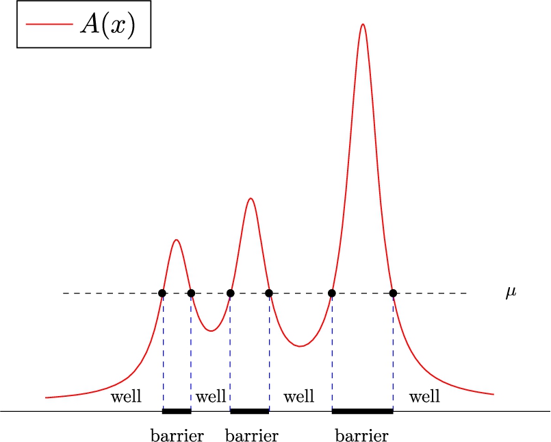
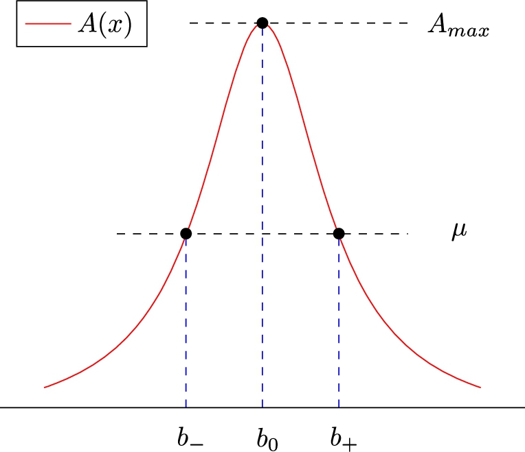
Let us denote by $R_{A} \subset R_{+}$ the range of the potential function $A : R \to R_{+}$ and take an $μ \in R_{A}$ . Assuming that equation $A (x) = μ$ has a finite number of solutions, these divide the domain $R$ of A to a finite number of intervals where $A (x) > μ$ and to (finitely many) intervals where $A (x) < μ$ (see Fig. 1). We call the former “barriers” and the latter“wells”. When an interval giving rise to a barrier (well) is bounded, we say that we have a barrier (well) of finite width or simply a finite barrier (well). Correspondingly, when we have unbounded intervals, we are in the presence of infinite barriers (or wells), i.e. barriers (wells) of infinite width.

Fig. 1.

Barriers and wells for a potential A at a specific energy level μ.

Next, in paragraph §5, we study the semiclassical spectrum of our operator with multiple potential humps. After the introduction of the necessary notation in §4.1, we show in paragraphs §§4.2–4.4 how our problem can be transformed to one where Olver’s theory (as adapted in sections §§2–3) can be applied. The results about the EVs and their corresponding quantization conditions are presented in §5.1. We show that for each EV there exists at least one barrier for which an associated Bohr-Sommerfeld quantization condition can be obtained, essentially in the same way as for the one barrier problem. Also, we establish a one-to-one correspondence between the EVs of the Dirac operator $D_{ℏ}$ lying in $i R$ (i.e. imaginary axis) and their WKB approximations.

The last component of the semiclassical scattering data is the reflection coefficient. This has been already studied in [9]; nothing changes in the multi-humped case. For the sake of completeness we present it briefly in paragraph §6 (the reflection coefficient away from zero is presented in §6.1 while the behavior closer to zero is found in §6.2).

In Section A of the appendix we show that Assumption 4.3 is not necessary when A is smooth. Then, since the motivation of our problem is the application to the semiclassical NLS, we discuss the effect of our direct scattering estimates to the inverse scattering problem in Section B of the appendix. It turns out that the asymptotic analysis of the inverse problem already conducted for the bell-shaped case in [11] and [12] is still relevant. The main change affects the new density of eigenvalues, which fortunately still retains its nice properties that enable the asymptotic analysis of the associated Riemann–Hilbert factorization problem.

For the sake of the reader, as the approximate solutions to our problems involve Airy, Parabolic Cylinder Functions and modified Parabolic Cylinder Functions, we present all the necessary results concerning these in Sections C and D of the appendix. Finally, in Section E we present a theorem concerning integral equations which is the backbone of the theory that we use in order to arrive at our results.

Before we start our main exposition, we specify some notation used throughout our work.

Complex conjugation is denoted with a star superscript, “∗”; i.e. $z^{*}$ is the complex conjugate of z (we emphasize that a bar over a number, does not indicate its complex conjugate).

The letters c, C denote generically positive constants (unless specified otherwise), appearing mainly in estimates.

For the Wronskian of two functions f, g we use the symbol $W [f, g]$ .

The notation $f^{2} (x)$ denotes the square of the value of the function f at x; hence, the symbols $f^{2} (x)$ and $f {(x)}^{2}$ are used interchangeably and are not to be confused with the composition $f \circ f$ .

The transpose of a matrix M is denoted by $M^{T}$ .

For the complement of a set B we write $∁ (B)$ .

For a set $Σ \subseteq R$ , when we write $i Σ$ we mean the set ${i κ ∣ κ \in Σ} \subset C$ . Also, for $z_{1}, z_{2} \in C$ the set $[z_{1}, z_{2}] \subset C$ denotes the closed line segment starting at $z_{1}$ and ending at $z_{2}$ .

For the restriction of a function $f : R \to R$ to the interval $Δ \subseteq R$ we have $f |_{Δ} : Δ \to R$ .

The closure of a set $Σ \subseteq R$ is denoted by $clos (Σ)$ .

Take a set $Σ \subseteq R$ and consider a function $f : Σ \to R$ . The set $R_{f} = {f (x) ∣ x \in Σ} \subseteq R$ represents its range.

Unless otherwise specified, $f^{- 1}$ shall always denote the inverse of an invertible function f.

If T is an operator, then $σ (T)$ , $σ_{ess} (T)$ and $σ_{p} (T)$ denote its spectrum, essential (continuous) spectrum and point spectrum respectively.

2. Passage through a potential barrier

We start the investigation of the behavior of the solutions to the following equation which turns out to be equivalent to our spectral Dirac spectral problem (see $§ 4$ ) $\begin{matrix} (2.1) & \frac{d^{2} y}{d x^{2}} = {ℏ^{- 2} [μ^{2} - A^{2} (x)] + \frac{3}{4} {[\frac{A^{'} (x)}{A (x) + μ}]}^{2} - \frac{1}{2} \frac{A^{″} (x)}{A (x) + μ}} y \end{matrix}$ where $μ > 0$ and the potential function $A : R \to R_{+}$ is characterized by a barrier of finite width (also called finite barrier) in some bounded interval in $R$ . Precisely, we consider one of the following assumptions for A.

For the case where the finite barrier lies between two wells of finite width (called finite wells), we assume the following.

Assumption 2.1 (finite barrier & finite wells).

The function A is positive on some bounded interval $[x_{1}, x_{2}]$ in $R$ and has a unique extremum in $(x_{1}, x_{2})$ ; particularly, a maximum $A_{max} > 0$ at $b_{0} \in (x_{1}, x_{2})$ . Also A is assumed to be $C^{4}$ in $(x_{1}, x_{2})$ and of class $C^{5}$ in a neighborhood of $b_{0}$ . Additionally, $A^{'} (x) > 0$ for $x \in (x_{1}, b_{0})$ and $A^{'} (x) < 0$ for $x \in (b_{0}, x_{2})$ . At $b_{0}$ we have $A^{'} (b_{0}) = 0$ and $A^{″} (b_{0}) < 0$ . Furthermore, if we let $A_{*} = max {A (x_{1}), A (x_{2})}$ and take $μ \in (A_{*}, A_{max}) \subset R_{+}$ , the equation $A (x) = μ$ has two solutions $b_{-} (μ)$ , $b_{+} (μ)$ in $(x_{1}, x_{2})$ . These satisfy $b_{-} < b_{+}$ , $A (x) > μ$ for $x \in (b_{-}, b_{+})$ and $A (x) < μ$ for $x \in (x_{1}, b_{-}) \cup (b_{+}, x_{2})$ (the above imply $\pm A^{'} (b_{\pm}) < 0$ ). Finally, when $μ = A_{max}$ the two points $b_{-}$ , $b_{+}$ coalesce into one double root at $b_{0}$ .

On the other hand, if the finite barrier is surrounded by one or two infinite wells, we have the following variants of Assumption 2.1. In these cases, we need to put some additional decay assumptions on A, $A^{'}$ and $A^{″}$ at the infinite ends. Hence we have one of the following.

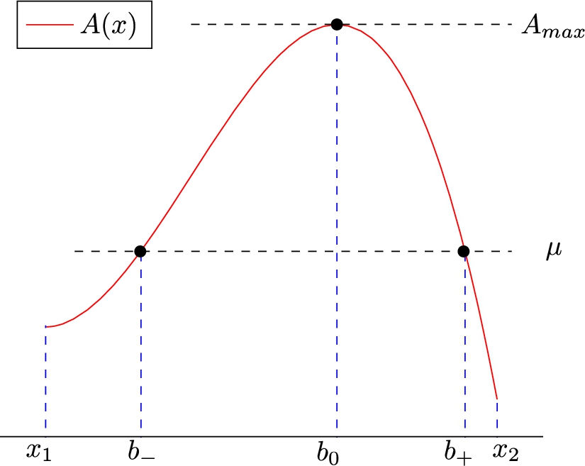
Assumption 2.2 (finite barrier & left infinite well).

The function A is positive on $(- \infty, x_{2}]$ in $R$ and ${lim}_{x ↓ - \infty} A (x) = 0$ . It has a unique extremum in $(- \infty, x_{2})$ ; particularly, a maximum $A_{max} > 0$ at $b_{0} \in (- \infty, x_{2})$ . Also A is assumed to be $C^{4}$ in $(- \infty, x_{2})$ and of class $C^{5}$ in a neighborhood of $b_{0}$ . Additionally, $A^{'} (x) > 0$ for $x \in (- \infty, b_{0})$ and $A^{'} (x) < 0$ for $x \in (b_{0}, x_{2})$ . At $b_{0}$ we have $A^{'} (b_{0}) = 0$ and $A^{″} (b_{0}) < 0$ . Furthermore, if we take $μ \in (A (x_{2}), A_{max}) \subset R_{+}$ , the equation $A (x) = μ$ has two solutions $b_{-} (μ)$ , $b_{+} (μ)$ in $(- \infty, x_{2})$ . These satisfy $b_{-} < b_{+}$ , $A (x) > μ$ for $x \in (b_{-}, b_{+})$ and $A (x) < μ$ for $x \in (- \infty, b_{-}) \cup (b_{+}, x_{2})$ (the above imply $\pm A^{'} (b_{\pm}) < 0$ ). When $μ = A_{max}$ the two points $b_{-}$ , $b_{+}$ coalesce into one double root at $b_{0}$ . 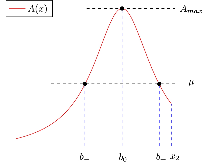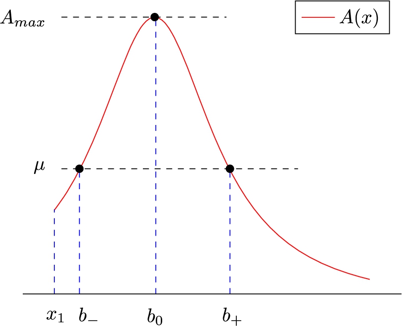Finally, there exists a number $τ > 0$ so that $\begin{array}{c} A (x) = O (\frac{1}{| x |^{1 + τ}}) as x ↓ - \infty \\ A^{'} (x) = O (\frac{1}{| x |^{2 + τ}}) as x ↓ - \infty \\ A^{″} (x) = O (\frac{1}{| x |^{3 + τ}}) as x ↓ - \infty \end{array}$

Assumption 2.3 (finite barrier & right infinite well).

The function A is positive on some interval $[x_{1}, + \infty)$ in $R$ and ${lim}_{x ↑ + \infty} A (x) = 0$ . It has a unique extremum in $(x_{1}, + \infty)$ ; particularly, a maximum $A_{max} > 0$ at $b_{0} \in (x_{1}, + \infty)$ . Also A is assumed to be $C^{4}$ in $(x_{1}, + \infty)$ and of class $C^{5}$ in a neighborhood of $b_{0}$ . Additionally, $A^{'} (x) > 0$ for $x \in (x_{1}, b_{0})$ and $A^{'} (x) < 0$ for $x \in (b_{0}, + \infty)$ . At $b_{0}$ we have $A^{'} (b_{0}) = 0$ and $A^{″} (b_{0}) < 0$ . Furthermore, if we take $μ \in (A (x_{1}), A_{max}) \subset R_{+}$ , the equation $A (x) = μ$ has two solutions $b_{-} (μ)$ , $b_{+} (μ)$ in $(x_{1}, + \infty)$ . These satisfy $b_{-} < b_{+}$ , $A (x) > μ$ for $x \in (b_{-}, b_{+})$ and $A (x) < μ$ for $x \in (x_{1}, b_{-}) \cup (b_{+}, + \infty)$ (the above imply $\pm A^{'} (b_{\pm}) < 0$ ). When $μ = A_{max}$ the two points $b_{-}$ , $b_{+}$ coalesce into one double root at $b_{0}$ . Finally, there exists a number $τ > 0$ so that $\begin{array}{c} A (x) = O (\frac{1}{x^{1 + τ}}) as x ↑ + \infty \\ A^{'} (x) = O (\frac{1}{x^{2 + τ}}) as x ↑ + \infty \\ A^{″} (x) = O (\frac{1}{x^{3 + τ}}) as x ↑ + \infty \end{array}$

Assumption 2.4 (finite barrier & two infinite wells).

The function A is positive on $R$ and ${lim}_{x \to \pm \infty} A (x) = 0$ . It has a unique extremum in $(- \infty, + \infty)$ ; particularly, a maximum $A_{max} > 0$ at $b_{0} \in (- \infty, + \infty)$ . Also A is assumed to be $C^{4}$ in $(- \infty, + \infty)$ and of class $C^{5}$ in a neighborhood of $b_{0}$ . Additionally, $A^{'} (x) > 0$ for $x \in (- \infty, b_{0})$ and $A^{'} (x) < 0$ for $x \in (b_{0}, + \infty)$ . At $b_{0}$ we have $A^{'} (b_{0}) = 0$ and $A^{″} (b_{0}) < 0$ . Furthermore, if we take $μ \in (0, A_{max}) \subset R_{+}$ , the equation $A (x) = μ$ has two solutions $b_{-} (μ)$ , $b_{+} (μ)$ in $(- \infty, + \infty)$ . These satisfy $b_{-} < b_{+}$ , $A (x) > μ$ for $x \in (b_{-}, b_{+})$ and $A (x) < μ$ for $x \in (- \infty, b_{-}) \cup (b_{+}, + \infty)$ (the above imply $\pm A^{'} (b_{\pm}) < 0$ ). When $μ = A_{max}$ the two points $b_{-}$ , $b_{+}$ coalesce into one double root at $b_{0}$ . Finally, there exists a number $τ > 0$ so that $\begin{array}{c} A (x) = O (\frac{1}{| x |^{1 + τ}}) as x \to \pm \infty \\ A^{'} (x) = O (\frac{1}{| x |^{2 + τ}}) as x \to \pm \infty \\ A^{″} (x) = O (\frac{1}{| x |^{3 + τ}}) as x \to \pm \infty \end{array}$

Remark 2.5.
The case where A is an even function, satisfying Assumption 2.4 is treated in complete detail in [9].

2.1. The Liouville transform for a barrier

Fig. 2.

An example of a finite potential barrier surrounded by two finite wells.

Fig. 3.

An example of a finite potential barrier accompanied by an infinite well on the left and a finite well on the right.

Fig. 4.

An example of a finite potential barrier accompanied by an infinite well on the right and a finite well on the left.

Fig. 5.

An example of a finite potential barrier accompanied by two infinite wells.

We begin with the first one of the above assumptions. All the assumptions can be treated similarly. Assume 2.1 (see Fig. 2),2

For Assumtion 2.2, see Figure 3. Similarly, Figure 4 and Figure 5 correspond to Assumption 2.3 and Assumption 2.4 accordingly.

with

μ = A (b_{-}) = A (b_{+})

. We temporarily drop the subscript and set

\begin{array}{c} b_{+} \equiv b \\ I^{-} = (x_{1}, b_{0}), I^{+} = (b_{0}, x_{2}) \end{array}

and define

\begin{matrix} (2.2) & G^{\pm} = {(A |_{clos (I^{\pm})})}^{- 1} . \end{matrix}

Take an arbitrary

μ_{1} \in (A_{*}, A_{max})

and consider the

b_{1} \in (b_{0}, G^{+} (A_{*}))

so that

A (b_{1}) = μ_{1}

(cf. Assumption 2.1 and (2.2)); then

μ \in [μ_{1}, A_{max}]

implies

b \in [b_{0}, b_{1}]

. For every

ℏ > 0

, equation (2.1) reads

\begin{matrix} (2.3) & \frac{d^{2} y}{d x^{2}} = [ℏ^{- 2} f (x, b) + g (x, b)] y, (x, b) \in (x_{1}, x_{2}) \times [b_{0}, b_{1}] \end{matrix}

in which the functions f and g satisfy

\begin{matrix} (2.4) & f (x, b) = A^{2} (b) - A^{2} (x) \end{matrix}

and

\begin{matrix} (2.5) & g (x, b) = \frac{3}{4} {[\frac{A^{'} (x)}{A (x) + A (b)}]}^{2} - \frac{1}{2} \frac{A^{″} (x)}{A (x) + A (b)} . \end{matrix}

We see that our equation (2.3) has two turning points (cf. Definition 1.1) at

x = b_{\pm}

when

b \in (b_{0}, b_{1}]

coalescing into one double at

x = b_{0}

; then b becomes

b_{0}

Next, we introduce new variables X and ζ according to the Liouville transform $\begin{matrix} X = {\dot{x}}^{- \frac{1}{2}} y \end{matrix}$ where the dot signifies differentiation with respect to ζ. Equation (2.3) becomes $\begin{matrix} (2.6) & \frac{d^{2} X}{d ζ^{2}} = [ℏ^{- 2} {\dot{x}}^{2} f (x, b) + {\dot{x}}^{2} g (x, b) + {\dot{x}}^{\frac{1}{2}} \frac{d^{2}}{d ζ^{2}} ({\dot{x}}^{- \frac{1}{2}})] X . \end{matrix}$ Let us treat the noncritical case $μ \in [μ_{1}, A_{max})$ first; two turning points $b_{\pm}$ being present. In this case $f (\cdot, b)$ is negative in $(b_{-}, b_{+})$ and positive in $(x_{1}, b_{-}) \cup (b_{+}, x_{2})$ . Hence we prescribe $\begin{matrix} (2.7) & {\dot{x}}^{2} f (x, b) = ζ^{2} - α^{2} \end{matrix}$ where $α > 0$ is chosen in such a way that $x = b_{-}$ corresponds to $ζ = - α$ and $x = b_{+}$ to $ζ = α$ accordingly.

After integration, (2.7) yields $\begin{matrix} (2.8) & \int_{b_{-}}^{x} {[- f (t, b)]}^{\frac{1}{2}} d t = \int_{- α}^{ζ} {(α^{2} - τ^{2})}^{\frac{1}{2}} d τ \end{matrix}$ provided that $b_{-} ⩽ x ⩽ b_{+}$ (notice that by taking these integration limits, $b_{-}$ corresponds to $- α$ ). For the remaining correspondence we require $\begin{matrix} \int_{b_{-}}^{b_{+}} {[- f (t, b)]}^{\frac{1}{2}} d t = \int_{- α}^{α} {(α^{2} - τ^{2})}^{\frac{1}{2}} d τ \end{matrix}$ and hence $\begin{matrix} (2.9) & α^{2} (μ) = \frac{2}{π} \int_{b_{-} (μ)}^{b_{+} (μ)} \sqrt{A^{2} (t) - μ^{2}} d t . \end{matrix}$ For every fixed value of ℏ, relation (2.9) defines α as a continuous and decreasing function of μ which vanishes as $μ ↑ A_{max}$ . Set $\begin{matrix} (2.10) & α_{1} = α (μ_{1}) > 0 . \end{matrix}$ Then $μ \in [μ_{1}, A_{max})$ implies $α \in (0, α_{1}]$ .

Next, from (2.8) we find $\begin{matrix} (2.11) & \int_{b_{-}}^{x} {[- f (t, b)]}^{\frac{1}{2}} d t = \frac{1}{2} α^{2} arccos (- \frac{ζ}{α}) + \frac{1}{2} ζ {(α^{2} - ζ^{2})}^{\frac{1}{2}} for b_{-} ⩽ x ⩽ b_{+} \end{matrix}$ with the principal value choice for the inverse cosine taking values in $[0, π]$ . For the remaining x-intervals, we integrate (2.7) to obtain $\begin{matrix} (2.12) & \int_{x}^{b_{-}} f {(t, b)}^{\frac{1}{2}} d t = - \frac{1}{2} α^{2} arcosh (- \frac{ζ}{α}) - \frac{1}{2} ζ {(ζ^{2} - α^{2})}^{\frac{1}{2}} for x_{1} < x ⩽ b_{-} \end{matrix}$ and $\begin{matrix} (2.13) & \int_{b_{+}}^{x} f {(t, b)}^{\frac{1}{2}} d t = - \frac{1}{2} α^{2} arcosh (\frac{ζ}{α}) + \frac{1}{2} ζ {(ζ^{2} - α^{2})}^{\frac{1}{2}} for b_{+} ⩽ x < x_{2} \end{matrix}$ with $arcosh (x) = ln (x + \sqrt{x^{2} - 1})$ for $x ⩾ 1$ .

Equations (2.11), (2.12) and (2.13) show that ζ is a continuous and increasing function of x which shows that there is a one-to-one correspondence between these two variables. Thus, if we set $\begin{matrix} (2.14) & ζ_{j} = lim_{x \to x_{j}} ζ (x) for j = 1, 2 \end{matrix}$ then $(x_{1}, x_{2})$ is mapped by ζ to $(ζ_{1}, ζ_{2})$ . Notice that $- \infty < ζ_{1} < 0 < ζ_{2} < + \infty$ since both $x_{1}$ , $x_{2}$ are finite by Assumption 2.1 (if $x_{1} = - \infty$ then $ζ_{1} = - \infty$ and if $x_{2} = + \infty$ then $ζ_{2} = + \infty$ ).

Remark 2.6.

In the critical case in which the two (simple) turning points coalesce into one (double) point, we get a limit of the above transformation with $b = b_{0}$ . In this case, the analogous relations to (2.11), (2.12), (2.13) are $\begin{array}{c} (2.15) & \int_{x}^{b_{0}} f {(t, b_{0})}^{\frac{1}{2}} d t = \frac{1}{2} ζ^{2} for x_{1} < x ⩽ b_{0} \\ (2.16) & \int_{b_{0}}^{x} f {(t, b_{0})}^{\frac{1}{2}} d t = \frac{1}{2} ζ^{2} for b_{0} ⩽ x < x_{2} \end{array}$ and $α = 0$ .

Finally, having in mind Remark 2.6, we substitute (2.7) in (2.6) and obtain the following proposition.

Proposition 2.7.

For every $ℏ > 0$ equation $\begin{matrix} \frac{d^{2} y}{d x^{2}} = [ℏ^{- 2} f (x, b) + g (x, b)] y, (x, b) \in (x_{1}, x_{2}) \times [b_{0}, b_{1}] \end{matrix}$ where f, g as in ( 2.4 ), ( 2.5 ) respectively, is transformed to the equation $\begin{matrix} (2.17) & \frac{d^{2} X}{d ζ^{2}} = [ℏ^{- 2} (ζ^{2} - α^{2}) + ψ (ζ, α)] X, (ζ, α) \in (ζ_{1}, ζ_{2}) \times [0, α_{1}] \end{matrix}$ in which ζ is given by the Liouville transform ( 2.7 ), α is given by ( 2.9 ), $ζ_{j}$ , $j = 1, 2$ are given by ( 2.14 ), $α_{1}$ as in ( 2.10 ) and the function $ψ (ζ, α)$ is given by the formula $\begin{matrix} (2.18) & ψ (ζ, α) = {\dot{x}}^{2} g (x, b) + {\dot{x}}^{\frac{1}{2}} \frac{d^{2}}{d ζ^{2}} ({\dot{x}}^{- \frac{1}{2}}) . \end{matrix}$

Since in the following paragraphs we shall be interested in approximate solutions of equation (2.17), we have the following.

Definition 2.8.

The function ψ found in the differential equation (2.17) shall be called the error term of this equation.

For the error term we have the following proposition.

Proposition 2.9.

The error term ψ can be written equivalently as $\begin{array}{rcl} ψ (ζ, α) & = & \frac{1}{4} \frac{3 ζ^{2} + 2 α^{2}}{{(ζ^{2} - α^{2})}^{2}} + \frac{1}{16} \frac{ζ^{2} - α^{2}}{f^{3} (x, b)} {4 f (x, b) f^{″} (x, b) - 5 {[f^{'} (x, b)]}^{2}} \\ (2.19) & + (ζ^{2} - α^{2}) \frac{g (x, b)}{f (x, b)} \end{array}$ where prime denotes differentiation with respect to x. The same formula can be used in the critical case of one double turning point simply by setting $b = b_{0}$ and $α = 0$ .

Proof.

Using (2.18), (2.5) and (2.7), simple algebraic manipulations shown that ψ takes the desired form. □

2.2. Continuity of the error term

In this subsection we prove a lemma concerning the continuity of the function $ψ (ζ, α)$ defined in (2.18) or (2.19). This fact will be used subsequently in §2.3 to prove the existence of approximate solutions of equation (2.17). We state it explicitly.

Lemma 2.10.
The function $ψ (ζ, α)$ defined in ( 2.18 ), is continuous in ζ and α in the region $(ζ_{1}, ζ_{2}) \times [0, α_{1}]$ of the $(ζ, α)$ -plane.
Proof.
For $x \in (x_{1}, x_{2})$ , $μ \in [μ_{1}, A_{max}]$ and $b \in [b_{0}, b_{1}]$ we introduce an auxiliary function p by setting $\begin{matrix} (2.20) & f (x, b) = (x - b_{-}) (x - b) p (x, b) . \end{matrix}$ Having in mind that $A (b_{-}) = A (b) = μ$ , we see that for $μ \in [μ_{1}, A_{max})$ $\begin{matrix} p (b_{\pm}, b) = \mp \frac{2 μ}{b - b_{-}} A^{'} (b_{\pm}) > 0 \end{matrix}$ while for $μ = A_{max}$ $\begin{matrix} p (b_{0}, b_{0}) = - A_{max} A^{″} (b_{0}) > 0 . \end{matrix}$

Our functions f, g and p defined by (2.4), (2.5) and (2.20) respectively satisfy the following properties
p, $\frac{\partial p}{\partial x}$ , $\frac{\partial^{2} p}{\partial x^{2}}$ and g are continuous functions of x and b (this means in x and b simultaneously and not separately) in the region $(x_{1}, x_{2}) \times [b_{0}, b_{1}]$

p is positive throughout the same region

$| \frac{\partial^{3} p}{\partial x^{3}} |$ is bounded in a neighborhood of the point $(x, b) = (b_{0}, b_{0})$ in the same region and

f is a non-increasing function of $b \in [b_{0}, b_{1}]$ when $x \in [b_{-}, b]$ .
Indeed, (i) and (iii) follow from (2.4), (2.5), (2.20) and the fact that A is in $C^{4}$ and of class $C^{5}$ in some neighborhood of $b_{0}$ (see Assumption 2.1). For (ii), use the definition (2.20) of p and recall the sign of f using (2.4). Finally (iv) is a consequence of (2.4) and the monotonicity of A in $[b_{0}, x_{2})$ (again cf. Assumption 2.1). By Lemma I in Olver’s paper [16], the function ψ defined by (2.18) is continuous in the corresponding region of the $(ζ, α)$ -plane. □

2.3. Approximate solutions in the barrier case

We return to equation (2.17) and state an existence theorem concerning its approximate solutions. To this goal, we need to assess the error. We do this by introducing an error-control function H along with a balancing function Ω.

Definition 2.11.
Define the balancing function Ω by $\begin{matrix} (2.21) & Ω (x) = 1 + | x |^{\frac{1}{3}} . \end{matrix}$ As an error-control function $H (ζ, α, ℏ)$ of equation (2.17) we consider any primitive of the function $\begin{matrix} \frac{ψ (ζ, α)}{Ω (ζ \sqrt{2 ℏ^{- 1}})} . \end{matrix}$

Furthermore, we need the notion of the variation of the error-control function H in a given interval. We have the following.
Definition 2.12.
Take $(γ, δ) \subseteq (ζ_{1}, ζ_{2}) \subseteq R$ (cf. (2.14)). The variation $V_{γ, δ} [H]$ in the interval $(γ, δ)$ of the error-control function H of equation (2.17) is defined by $\begin{matrix} V_{γ, δ} [H] (α, ℏ) = \int_{γ}^{δ} \frac{| ψ (t, α) |}{Ω (t \sqrt{2 ℏ^{- 1}})} d t . \end{matrix}$

Finally, for any $c ⩽ 0$ set $\begin{matrix} (2.22) & l_{1} (c) = sup_{x \in (0, + \infty)} {Ω (x) \frac{M {(x, c)}^{2}}{Γ (\frac{1}{2} - c)}} \end{matrix}$ where $M$ is a function defined in terms of Parabolic Cylinder Functions in section (D.1) of the appendix and Γ denotes the Gamma function. We note that the above supremum is finite for each value of c. This fact is a consequence of (2.21) and the first relation in (D.9). Furthermore, because the relations (D.9) hold uniformly in compact intervals of $(- \infty, 0]$ , the function $l_{1}$ is continuous.

We are now ready for the main theorem of this paragraph. Theorem 2.13.
For each value of $ℏ > 0$ the equation $\begin{matrix} \frac{d^{2} X}{d ζ^{2}} = [ℏ^{- 2} (ζ^{2} - α^{2}) + ψ (ζ, α)] X \end{matrix}$ has in the region $[0, ζ_{2}) \times [0, α_{1}]$ of the $(ζ, α)$ -plane, two solutions $Y_{+}$ and $Z_{+}$ satisfying $\begin{array}{c} (2.23) & Y_{+} (ζ, α, ℏ) = U (ζ \sqrt{2 ℏ^{- 1}}, - \frac{1}{2} ℏ^{- 1} α^{2}) + ε_{1} (ζ, α, ℏ) \\ (2.24) & Z_{+} (ζ, α, ℏ) = \overline{U} (ζ \sqrt{2 ℏ^{- 1}}, - \frac{1}{2} ℏ^{- 1} α^{2}) + ε_{2} (ζ, α, ℏ) \end{array}$ where U, $\overline{U}$ are the PCFs defined in appendix ( D.1 ). These two solutions $Y_{+}$ , $Z_{+}$ are continuous and have continuous first and second partial ζ-derivatives. The errors $ε_{1}$ , $ε_{2}$ in the relations above satisfy the estimates 3
³
The functions $E$ , $M$ and $N$ are related with the PCF theory found in appendix (D.1).

$\begin{array}{c} \frac{| ε_{1} (ζ, α, ℏ) |}{M (ζ \sqrt{2 ℏ^{- 1}}, - \frac{1}{2} ℏ^{- 1} α^{2})}, \frac{| \frac{\partial ε_{1}}{\partial ζ} (ζ, α, ℏ) |}{\sqrt{2 ℏ^{- 1}} N (ζ \sqrt{2 ℏ^{- 1}}, - \frac{1}{2} ℏ^{- 1} α^{2})} \\ (2.25) & ⩽ \frac{1}{E (ζ \sqrt{2 ℏ^{- 1}}, - \frac{1}{2} ℏ^{- 1} α^{2})} (exp {\frac{1}{2} {(π ℏ)}^{\frac{1}{2}} l_{1} (- \frac{1}{2} ℏ^{- 1} α^{2}) V_{ζ, ζ_{2}} [H] (α, ℏ)} - 1) \end{array}$ and $\begin{array}{c} \frac{| ε_{2} (ζ, α, ℏ) |}{M (ζ \sqrt{2 ℏ^{- 1}}, - \frac{1}{2} ℏ^{- 1} α^{2})}, \frac{| \frac{\partial ε_{2}}{\partial ζ} (ζ, α, ℏ) |}{\sqrt{2 ℏ^{- 1}} N (ζ \sqrt{2 ℏ^{- 1}}, - \frac{1}{2} ℏ^{- 1} α^{2})} \\ (2.26) & ⩽ E (ζ \sqrt{2 ℏ^{- 1}}, - \frac{1}{2} ℏ^{- 1} α^{2}) (exp {\frac{1}{2} {(π ℏ)}^{\frac{1}{2}} l_{1} (- \frac{1}{2} ℏ^{- 1} α^{2}) V_{0, ζ} [H] (α, ℏ)} - 1) . \end{array}$
Proof.
In order to prove this theorem, we rely on Theorem I in [16]. There, it is stated that it suffices to prove two things. First that the function ψ is continuous in the region $[0, ζ_{2}) \times [0, α_{1}]$ , a fact that has already been proven in §2.2 and second that the integral $\begin{matrix} (2.27) & V_{0, ζ_{2}} [H] (α, ℏ) = \int_{0}^{ζ_{2}} \frac{| ψ (t, α) |}{Ω (t \sqrt{2 ℏ^{- 1}})} d t \end{matrix}$ converges uniformly in α. But this is obvious since $ζ_{2} < + \infty$ . □
Remark 2.14.
If we were assuming either Assumption 2.3 or Assumption 2.4 we would have $ζ_{2} = + \infty$ . In such a case, Theorem 2.13 would still be true. To obtain it, we have to argue as in the proof of Theorem 6.1 in [9].

2.4. Asymptotics of the approximate solutions for the barrier

In order to extract the asymptotic behavior of the solutions $Y_{+} (ζ, α, ℏ)$ , $Z_{+} (ζ, α, ℏ)$ when $ℏ ↓ 0$ , we need to determine the asymptotic form of the error bounds (2.25), (2.26) examining closely $l_{1} (- \frac{1}{2} ℏ^{- 1} α^{2})$ and $V_{0, ζ_{2}} [H] (α, ℏ)$ as $ℏ ↓ 0$ .

Let us deal with the noncritical case $α \in (0, α_{1}]$ first. By applying the same analysis found in §8 of [9] we obtain $\begin{matrix} (2.28) & l_{1} (- \frac{1}{2} ℏ^{- 1} α^{2}) = O (1) as ℏ ↓ 0 . \end{matrix}$ Next, we examine $V_{0, ζ_{2}} [H] (α, ℏ)$ . Again in §8 of [9] it is shown that $\begin{aligned} (2.29) & V_{0, ζ_{2}} [H] (α, ℏ) = \int_{0}^{ζ_{2}} \frac{| ψ (t, α) |}{1 + {(t \sqrt{2 ℏ^{- 1}})}^{\frac{1}{3}}} d t = O (ℏ^{1 / 6}) as ℏ ↓ 0 \end{aligned}$ when $ζ_{2} = + \infty$ . Clearly the same asymptotics hold in the case when $ζ_{2} < + \infty$ too.

The last two relations applied to (2.25) and (2.26) supply us with the desired results as $ℏ ↓ 0$ $\begin{array}{c} (2.30) & ε_{1} (ζ, α, ℏ) = \frac{M (ζ \sqrt{2 ℏ^{- 1}}, - \frac{1}{2} ℏ^{- 1} α^{2})}{E (ζ \sqrt{2 ℏ^{- 1}}, - \frac{1}{2} ℏ^{- 1} α^{2})} O (ℏ^{\frac{2}{3}}) \\ ε_{2} (ζ, α, ℏ) = E (ζ \sqrt{2 ℏ^{- 1}}, - \frac{1}{2} ℏ^{- 1} α^{2}) M (ζ \sqrt{2 ℏ^{- 1}}, - \frac{1}{2} ℏ^{- 1} α^{2}) O (ℏ^{\frac{2}{3}}) \\ \frac{\partial ε_{1}}{\partial ζ} (ζ, α, ℏ) = \frac{N (ζ \sqrt{2 ℏ^{- 1}}, - \frac{1}{2} ℏ^{- 1} α^{2})}{E (ζ \sqrt{2 ℏ^{- 1}}, - \frac{1}{2} ℏ^{- 1} α^{2})} O (ℏ^{\frac{1}{6}}) \\ \frac{\partial ε_{2}}{\partial ζ} (ζ, α, ℏ) = E (ζ \sqrt{2 ℏ^{- 1}}, - \frac{1}{2} ℏ^{- 1} α^{2}) N (ζ \sqrt{2 ℏ^{- 1}}, - \frac{1}{2} ℏ^{- 1} α^{2}) O (ℏ^{\frac{1}{6}}) \end{array}$ uniformly for $ζ \in [0, ζ_{2})$ and $α \in (0, α_{1}]$ .

Remark 2.15.
In the special case $α = 0$ (i.e. when equation (2.17) has a double turning point at $ζ = 0$ ), $l_{1} (0)$ is independent of ℏ. Using the definition (2.21) of Ω, we see that we have a similar estimate to (2.29); namely $V_{0, ζ_{2}} [H] (0, ℏ) = O (ℏ^{\frac{1}{6}})$ as $ℏ ↓ 0$ . Hence the error estimates above still hold for the case $α = 0$ .

2.5. Connection formulae for a barrier

We can determine the asymptotic behavior of $Y_{+}$ , $Z_{+}$ for small $ℏ > 0$ and $ζ < 0$ by establishing appropriate connection formulae. We can replace ζ by $- ζ$ in Theorem 2.13 to ensure two more solutions $Y_{-}$ , $Z_{-}$ of equation (2.17) satisfying as $ℏ ↓ 0$ $\begin{array}{c} (2.31) & \begin{array}{c} Y_{-} (ζ, α, ℏ) = U (- ζ \sqrt{2 ℏ^{- 1}}, - \frac{1}{2} ℏ^{- 1} α^{2}) + \frac{M (- ζ \sqrt{2 ℏ^{- 1}}, - \frac{1}{2} ℏ^{- 1} α^{2})}{E (- ζ \sqrt{2 ℏ^{- 1}}, - \frac{1}{2} ℏ^{- 1} α^{2})} O (ℏ^{\frac{2}{3}}) \\ \begin{aligned} Z_{-} (ζ, α, ℏ) & = \overline{U} (- ζ \sqrt{2 ℏ^{- 1}}, - \frac{1}{2} ℏ^{- 1} α^{2}) \\ + E (- ζ \sqrt{2 ℏ^{- 1}}, - \frac{1}{2} ℏ^{- 1} α^{2}) M (- ζ \sqrt{2 ℏ^{- 1}}, - \frac{1}{2} ℏ^{- 1} α^{2}) O (ℏ^{\frac{2}{3}}) \end{aligned} \end{array} \end{array}$ uniformly for $ζ \in (ζ_{1}, 0]$ and $α \in [0, α_{1}]$ .

Remark 2.16.
The two sets ${Y_{+}, Z_{+}}$ and ${Y_{-}, Z_{-}}$ consist of two linearly independent functions. This can be seen by their Wronskians. For example, using (D.3) we have $\begin{matrix} W [U (\cdot, - \frac{1}{2} ℏ^{- 1} α^{2}), \overline{U} (\cdot, - \frac{1}{2} ℏ^{- 1} α^{2})] = \sqrt{\frac{2}{π}} Γ (\frac{1}{2} + \frac{1}{2} ℏ^{- 1} α^{2}) \end{matrix}$ Using this and (2.23), (2.24) we see that $W [Y_{+}, Z_{+}] \neq 0$ . Similarly, we have $W [Y_{-}, Z_{-}] \neq 0$ as well.

We express $Y_{+}$ , $Z_{+}$ in terms of $Y_{-}$ , $Z_{-}$ . So for $(ζ, α) \in (ζ_{1}, 0] \times [0, α_{1}]$ we may write $\begin{array}{c} (2.32) & Y_{+} (ζ, α, ℏ) = σ_{11} (α, ℏ) Y_{-} (ζ, α, ℏ) + σ_{12} (α, ℏ) Z_{-} (ζ, α, ℏ) \\ (2.33) & Z_{+} (ζ, α, ℏ) = σ_{21} (α, ℏ) Y_{-} (ζ, α, ℏ) + σ_{22} (α, ℏ) Z_{-} (ζ, α, ℏ) . \end{array}$ The connection will become clear once we find approximations for the coefficients $σ_{i j}$ , $i, j = 1, 2$ in the linear relations (2.32) and (2.33). We evaluate at $ζ = 0$ equations (2.32), (2.33) and their derivatives. After algebraic manipulations we obtain $\begin{array}{c} σ_{11} (α, ℏ) = \frac{W [Y_{+} (\cdot, α, ℏ), Z_{-} (\cdot, α, ℏ)] (0)}{W [Y_{-} (\cdot, α, ℏ), Z_{-} (\cdot, α, ℏ)] (0)} \\ σ_{12} (α, ℏ) = - \frac{W [Y_{+} (\cdot, α, ℏ), Y_{-} (\cdot, α, ℏ)] (0)}{W [Y_{-} (\cdot, α, ℏ), Z_{-} (\cdot, α, ℏ)] (0)} \\ σ_{21} (α, ℏ) = \frac{W [Z_{+} (\cdot, α, ℏ), Z_{-} (\cdot, α, ℏ)] (0)}{W [Y_{-} (\cdot, α, ℏ), Z_{-} (\cdot, α, ℏ)] (0)} \\ σ_{22} (α, ℏ) = - \frac{W [Z_{+} (\cdot, α, ℏ), Y_{-} (\cdot, α, ℏ)] (0)}{W [Y_{-} (\cdot, α, ℏ), Z_{-} (\cdot, α, ℏ)] (0)} . \end{array}$

Now set $\begin{matrix} φ (α, ℏ) = (1 + ℏ^{- 1} α^{2}) \frac{π}{4} . \end{matrix}$ By using the results and properties of Parabolic Cylinder Functions and their auxiliary functions from Section D.1 in the appendix, we find that as $ℏ ↓ 0$ $\begin{array}{c} Y_{1} (0, α, ℏ) = M (0) [sin φ (α, ℏ) + O (ℏ^{\frac{2}{3}})] \\ Y_{2} (0, α, ℏ) = M (0) [cos φ (α, ℏ) + O (ℏ^{\frac{2}{3}})] \\ Y_{3} (0, α, ℏ) = M (0) [sin φ (α, ℏ) + O (ℏ^{\frac{2}{3}})] \\ Y_{4} (0, α, ℏ) = M (0) [cos φ (α, ℏ) + O (ℏ^{\frac{2}{3}})] \\ {\dot{Y}}_{1} (0, α, ℏ) = - \sqrt{2 ℏ^{- 1}} N (0) [cos φ (α, ℏ) + O (ℏ^{\frac{2}{3}})] \\ {\dot{Y}}_{2} (0, α, ℏ) = \sqrt{2 ℏ^{- 1}} N (0) [sin φ (α, ℏ) + O (ℏ^{\frac{2}{3}})] \\ {\dot{Y}}_{3} (0, α, ℏ) = \sqrt{2 ℏ^{- 1}} N (0) [cos φ (α, ℏ) + O (ℏ^{\frac{2}{3}})] \\ {\dot{Y}}_{4} (0, α, ℏ) = - \sqrt{2 ℏ^{- 1}} N (0) [sin φ (α, ℏ) + O (ℏ^{\frac{2}{3}})] . \end{array}$ Recall that the dot denotes differentiation with respect to ζ. Finally, using these estimates we obtain as $ℏ ↓ 0$ $\begin{matrix} (2.34) & \begin{aligned} σ_{11} (α, ℏ) & = sin (\frac{1}{2} π ℏ^{- 1} α^{2}) + O (ℏ^{\frac{2}{3}}) \\ σ_{12} (α, ℏ) & = cos (\frac{1}{2} π ℏ^{- 1} α^{2}) + O (ℏ^{\frac{2}{3}}) \\ σ_{21} (α, ℏ) & = cos (\frac{1}{2} π ℏ^{- 1} α^{2}) + O (ℏ^{\frac{2}{3}}) \\ σ_{22} (α, ℏ) & = - sin (\frac{1}{2} π ℏ^{- 1} α^{2}) + O (ℏ^{\frac{2}{3}}) \end{aligned} \end{matrix}$ uniformly for $α \in [0, α_{1}]$ .
2.6. Applications in the barrier case

We assume 2.1 (similar arguments hold for the other cases as well). Recalling (2.9), we define the following integral.

Definition 2.17.
The function $\begin{matrix} (2.35) & Φ (μ) = \frac{π}{2} α^{2} (μ) = \int_{b_{-} (μ)}^{b_{+} (μ)} \sqrt{A {(x)}^{2} - μ^{2}} d x \end{matrix}$ is called the abbreviated action integral.

It is easily checked that Φ is of class $C^{1}$ . Differentiating relation (2.35) while using $A (b_{\pm}) = μ$ , we obtain $\begin{matrix} (2.36) & \frac{d Φ (μ)}{d μ} = - 2 μ \int_{b_{-} (μ)}^{b_{+} (μ)} {[A {(x)}^{2} - μ^{2}]}^{- \frac{1}{2}} d x < 0 . \end{matrix}$

The asymptotic behavior as $ℏ ↓ 0$ of an arbitrary non-trivial real solution X of equation (2.17) on the ζ-interval corresponding to the finite x-barrier $(b_{-}, b_{+})$ of A, can be examined through the functions $Y_{+}$ , $Z_{+}$ and $Y_{-}$ , $Z_{-}$ . Since ${Y_{+}, Z_{+}}$ and ${Y_{-}, Z_{-}}$ are two sets of linearly independent functions (cf. Remark 2.16), for X we can write $\begin{aligned} X (ζ, α, ℏ) & = γ_{+} (α, ℏ) Y_{+} (ζ, α, ℏ) + δ_{+} (α, ℏ) Z_{+} (ζ, α, ℏ) \\ (2.37) & = γ_{-} (α, ℏ) Y_{-} (ζ, α, ℏ) + δ_{-} (α, ℏ) Z_{-} (ζ, α, ℏ) \end{aligned}$ for some $γ_{\pm} (α, ℏ), δ_{\pm} (α, ℏ) \in R$ . We put $\begin{array}{c} (2.38) & \begin{array}{c} v_{\pm} (α, ℏ) = \sqrt{γ_{\pm} {(α, ℏ)}^{2} + δ_{\pm} {(α, ℏ)}^{2}} \\ γ_{\pm} (α, ℏ) = v_{\pm} (α, ℏ) cos ξ_{\pm} (α, ℏ) \\ \begin{aligned} δ_{\pm} (α, ℏ) & = v_{\pm} (α, ℏ) sin ξ_{\pm} (α, ℏ) \\ ξ_{\pm} (α, ℏ) \in R / (2 π Z) \end{aligned} \end{array} \end{array}$ and define $\begin{matrix} (2.39) & ξ (μ, ℏ) = ξ_{+} (α (μ), ℏ) + ξ_{-} (α (μ), ℏ) . \end{matrix}$ Recall that α is function of μ. Whence we can see that $ξ_{\pm}$ , ξ depend on μ. Sometimes we shall simply write $ξ_{\pm} (μ, ℏ)$ meaning $ξ_{\pm} (α (μ), ℏ)$ .

The ideas that follow are essentially the same as those used in the derivation of the Bohr-Sommerfeld quantization condition found in §10 of [9]. We start with a theorem.
Theorem 2.18.
Under Assumption 2.1 , there is a non-negative integer $n = n (μ, ℏ)$ such that the functions Φ and ξ in ( 2.35 ) and ( 2.39 ) respectively satisfy the formula $\begin{matrix} (2.40) & Φ (μ) = [(2 n + 1) \frac{π}{2} - ξ (μ, ℏ)] ℏ + O (ℏ^{\frac{5}{3}}) as ℏ ↓ 0 . \end{matrix}$
Proof.
Using (2.37) and (2.38) we have $\begin{aligned} 0 & = W [X, X] = W [γ_{+} Z_{+} + δ_{+} Y_{+}, γ_{-} Z_{-} + δ_{-} Y_{-}] \\ = v_{+} v_{-} W [Y_{-}, Z_{-}] (- σ_{12} cos ξ_{+} cos ξ_{-} + σ_{11} cos ξ_{+} sin ξ_{-} \\ - σ_{22} sin ξ_{+} cos ξ_{-} + σ_{21} sin ξ_{+} sin ξ_{-}) \end{aligned}$ (we have suppressed the dependence on α and ℏ for notational simplicity). From (2.38), (2.34) and (2.39) $\begin{matrix} cos [ℏ^{- 1} Φ (μ) + ξ (μ, ℏ)] = O (ℏ^{\frac{2}{3}}) as ℏ ↓ 0 \end{matrix}$ from which the result follows. □

If $ξ (μ, ℏ) = 0 (mod π)$ , then relation (2.40) reduces to the Bohr-Sommerfeld quantization condition. In particular, this is true if $ξ_{\pm} (μ, ℏ) = 0 (mod π)$ at both turning points $b_{\pm} (μ)$ . We state this explicitly.
Theorem 2.19.
Under Assumption 2.1 , suppose that a non-trivial real solution of ( 2.17 ) satisfies ( 2.37 ) and ( 2.38 ) with $ξ_{\pm} (μ, ℏ) = 0 (mod π)$ . Then function Φ in ( 2.35 ) satisfies the condition $\begin{matrix} (2.41) & cos [ℏ^{- 1} Φ (μ)] = O (ℏ^{\frac{2}{3}}) as ℏ ↓ 0 \end{matrix}$ whence $\begin{matrix} (2.42) & Φ (μ) = π (n + \frac{1}{2}) ℏ + O (ℏ^{\frac{5}{3}}) as ℏ ↓ 0 \end{matrix}$ for some non-negative integer $n = n (μ, ℏ)$ .
Remark 2.20.
It is possible that $ξ_{\pm} (μ, ℏ) = 0 (mod π)$ only for ℏ in some set $Σ \subset R_{+}$ such that $0 \in clos (Σ)$ . Then conditions (2.41), (2.42) are also satisfied for $ℏ \in Σ$ .

What follows is a result converse to Theorem 2.19. Theorem 2.21.
Under Assumption 2.1 , suppose that for some non-negative integer n, the point $π (n + \frac{1}{2}) ℏ$ lies in $(0, \frac{π}{2} α_{1}^{2})$ . Then there exists a value $\tilde{μ} = \tilde{μ} (n, ℏ)$ such that $\begin{matrix} Φ (\tilde{μ}) = π (n + \frac{1}{2}) ℏ + O (ℏ^{\frac{5}{3}}) as ℏ ↓ 0 \end{matrix}$ and $\begin{matrix} Y_{+} (ζ, α (\tilde{μ}), ℏ) = σ_{11} (α (\tilde{μ}), ℏ) Y_{-} (ζ, α (\tilde{μ}), ℏ) \end{matrix}$ where $\begin{matrix} σ_{11} (α (\tilde{μ}), ℏ) = {(- 1)}^{n} + O (ℏ^{\frac{2}{3}}) as ℏ ↓ 0 . \end{matrix}$
Proof.
Recall the connection coefficients $σ_{i j}$ , $i, j = 1, 2$ from §2.5 and define the function $\begin{matrix} (2.43) & σ (μ, ℏ) = σ_{12} (α (μ), ℏ) . \end{matrix}$ From (2.32), it is enough to show that σ vanishes for some $\tilde{μ} = \tilde{μ} (n, ℏ)$ satisfying $\begin{matrix} | Φ (\tilde{μ}) - π (n + \frac{1}{2}) ℏ | ⩽ C ℏ^{\frac{5}{3}} \end{matrix}$ where C does not depend neither on n nor on ℏ. Then, the rest follow from the first asymptotic relation in (2.34).

From (2.36) we know that Φ maps a neighborhood of $\tilde{μ}$ in a one-to-one way onto a neighborhood of $Φ (\tilde{μ})$ . Let $X = Φ (μ)$ and set $\begin{matrix} χ (X, ℏ) = σ (Φ^{- 1} (X), ℏ) - cos (ℏ^{- 1} X) . \end{matrix}$ By definition (2.43) of σ and the second relation in (2.34) we have $\begin{matrix} | χ (X, ℏ) | ⩽ C ℏ^{\frac{2}{3}} \end{matrix}$ for a constant C independent of ℏ and $X$ . With the above definitions, our equation now reads $\begin{aligned} 0 & = σ (μ, ℏ) \\ = χ (X, ℏ) + cos (ℏ^{- 1} X) . \end{aligned}$ So this equation has to have a solution $\tilde{X} = \tilde{X} (n, ℏ) = Φ (\tilde{μ} (n, ℏ))$ satisfying the estimate $\begin{matrix} | \tilde{X} - π (n + \frac{1}{2}) ℏ | ⩽ C ℏ^{\frac{5}{3}} . \end{matrix}$

A change of variables $s = ℏ^{- 1} X$ transforms our problem to the equivalent assertion that equation $\begin{matrix} (2.44) & χ (ℏ s, ℏ) + cos s = 0 \end{matrix}$ has to have a solution with respect to s, namely $\tilde{s} = \tilde{s} (n, ℏ) = ℏ^{- 1} \tilde{X}$ , such that $\begin{matrix} (2.45) & | \tilde{s} - π (n + \frac{1}{2}) | ⩽ C ℏ^{\frac{2}{3}} . \end{matrix}$ But this is true because $\begin{matrix} χ (ℏ s, ℏ) = O (ℏ^{\frac{2}{3}}) as ℏ ↓ 0 . \end{matrix}$ □

3. The case of one potential well

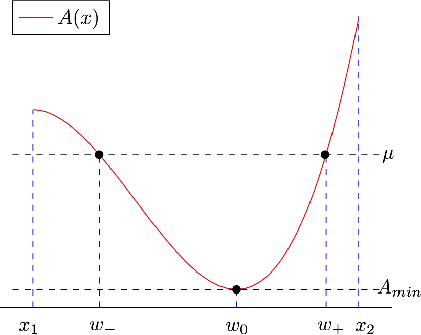
In this section we are interested in the solutions of equation $\begin{matrix} (3.1) & \frac{d^{2} y}{d x^{2}} = {ℏ^{- 2} [μ^{2} - A^{2} (x)] + \frac{3}{4} {[\frac{A^{'} (x)}{A (x) + μ}]}^{2} - \frac{1}{2} \frac{A^{″} (x)}{A (x) + μ}} y \end{matrix}$ where $μ > 0$ and the potential function $A : R \to R_{+}$ behaves as a finite well (a well of finite width) in some bounded interval in $R$ . We assume the following (see Fig. 6).

Assumption 3.1.
The function A is positive on some bounded interval $[x_{1}, x_{2}]$ in $R$ and has a unique extremum in $(x_{1}, x_{2})$ ; particularly, a minimum $A_{min} > 0$ at $w_{0} \in (x_{1}, x_{2})$ . Also A is assumed to be $C^{4}$ in $(x_{1}, x_{2})$ and of class $C^{5}$ in a neighborhood of $w_{0}$ . Additionally, $A^{'} (x) < 0$ for $x \in (x_{1}, w_{0})$ and $A^{'} (x) > 0$ for $x \in (w_{0}, x_{2})$ . At $w_{0}$ , we have $A^{'} (w_{0}) = 0$ and $A^{″} (w_{0}) > 0$ . Furthermore, if we let $A_{* } = min {A (x_{1}), A (x_{2})}$ and take $μ \in (A_{min}, A_{ *}) \subset R_{+}$ , the equation $A (x) = μ$ has two solutions $w_{-} (μ)$ , $w_{+} (μ)$ in $(x_{1}, x_{2})$ . These satisfy $w_{-} < w_{+}$ , $A (x) < μ$ for $x \in (w_{-}, w_{+})$ and $A (x) > μ$ for $x \in (x_{1}, w_{-}) \cup (w_{+}, x_{2})$ (the above imply $\pm A^{'} (w_{\pm}) > 0$ ). Finally, when $μ = A_{min}$ the two points $w_{-}$ , $w_{+}$ coalesce into one double root at $w_{0}$ .

3.1. The Liouville transform for the case of a well

Fig. 6.

An example of a potential well between $w_{-}$ and $w_{+}$ .

Let us first fix some notation. We set $\begin{array}{c} w_{-} \equiv w \\ J^{-} = (x_{1}, w_{0}), J^{+} = (w_{0}, x_{2}) \end{array}$ and define $\begin{matrix} (3.2) & G^{\pm} = {(A |_{clos (J^{\pm})})}^{- 1} . \end{matrix}$ We take an arbitrary $μ_{1} \in (A_{min}, A_{* *})$ and consider the $w_{- 1} \in (G^{-} (A_{* *}), w_{0})$ such that $A (w_{- 1}) = μ_{1}$ ; then $μ \in [A_{min}, μ_{1}]$ implies $w \in [w_{- 1}, w_{0}]$ . For every $ℏ > 0$ our equation (3.1) reads $\begin{matrix} (3.3) & \frac{d^{2} y}{d x^{2}} = [ℏ^{- 2} f (x, w) + g (x, w)] y, (x, w) \in (x_{1}, x_{2}) \times [w_{- 1}, w_{0}] \end{matrix}$ in which the functions f and g satisfy $\begin{matrix} (3.4) & f (x, w) = A^{2} (w) - A^{2} (x) \end{matrix}$ and $\begin{matrix} (3.5) & g (x, w) = \frac{3}{4} {[\frac{A^{'} (x)}{A (x) + A (w)}]}^{2} - \frac{1}{2} \frac{A^{″} (x)}{A (x) + A (w)} . \end{matrix}$ Observe that our equation possesses two simple turning points at $x = w_{\pm}$ when $w \in [w_{- 1}, w_{0})$ which combine into one double at $x = w_{0}$ when w equals $w_{0}$ .

We introduce new variables X and ζ according to the Liouville transform $\begin{matrix} X = {\dot{x}}^{- \frac{1}{2}} y \end{matrix}$ where the dot denotes differentiation with respect to ζ. Equation (3.3) becomes $\begin{matrix} (3.6) & \frac{d^{2} X}{d ζ^{2}} = [ℏ^{- 2} {\dot{x}}^{2} f (x, w) + {\dot{x}}^{2} g (x, w) + {\dot{x}}^{\frac{1}{2}} \frac{d^{2}}{d ζ^{2}} ({\dot{x}}^{- \frac{1}{2}})] X . \end{matrix}$ We begin with the noncritical case $μ \in (A_{min}, μ_{1}]$ with two turning points $w_{\pm}$ . In this case $f (\cdot, w)$ is positive in $(w_{-}, w_{+})$ and negative in $(x_{1}, w_{-}) \cup (w_{+}, x_{2})$ . Hence we prescribe $\begin{matrix} (3.7) & {\dot{x}}^{2} f (x, w) = β^{2} - ζ^{2} \end{matrix}$ where $β > 0$ is chosen in such a way that $x = w_{-}$ corresponds to $ζ = - β$ and $x = w_{+}$ to $ζ = β$ accordingly.

The integration of (3.7) yields $\begin{matrix} (3.8) & \int_{w}^{x} f {(t, w)}^{\frac{1}{2}} d t = \int_{- β}^{ζ} {(β^{2} - τ^{2})}^{\frac{1}{2}} d τ \end{matrix}$ provided that $w_{-} ⩽ x ⩽ w_{+}$ (notice that by taking these integration limits, $w_{-}$ corresponds to $- β$ ). For the remaining correspondence we require $\begin{matrix} \int_{w_{-}}^{w_{+}} f {(t, w)}^{\frac{1}{2}} d t = \int_{- β}^{β} {(β^{2} - τ^{2})}^{\frac{1}{2}} d τ \end{matrix}$ yielding $\begin{matrix} (3.9) & β^{2} (μ) = \frac{2}{π} \int_{w_{-} (μ)}^{w_{+} (μ)} \sqrt{μ^{2} - A^{2} (t)} d t . \end{matrix}$

For every fixed value of ℏ, relation (3.9) defines β as a continuous and increasing function of μ which vanishes as $w ↓ A_{min}$ . Set $\begin{matrix} (3.10) & β_{1} = β (w_{- 1}) > 0 . \end{matrix}$ Then $μ \in (A_{min}, μ_{1}]$ implies $β \in (0, β_{1}]$ .

Next, from (3.8) we find $\begin{matrix} (3.11) & \int_{w_{-}}^{x} f {(t, w)}^{\frac{1}{2}} d t = \frac{1}{2} α^{2} arccos (- \frac{ζ}{α}) + \frac{1}{2} ζ {(α^{2} - ζ^{2})}^{\frac{1}{2}} for w_{-} ⩽ x ⩽ w_{+} \end{matrix}$ with the principal value choice for the inverse cosine taking values in $[0, π]$ . For the remaining x-intervals, we integrate (3.7) to obtain $\begin{matrix} (3.12) & \int_{x}^{w_{-}} {[- f (t, w)]}^{\frac{1}{2}} d t = - \frac{1}{2} α^{2} arcosh (- \frac{ζ}{α}) - \frac{1}{2} ζ {(ζ^{2} - α^{2})}^{\frac{1}{2}} for x_{1} < x ⩽ w_{-} \end{matrix}$ and $\begin{matrix} (3.13) & \int_{w_{+}}^{x} {[- f (t, w)]}^{\frac{1}{2}} d t = - \frac{1}{2} α^{2} arcosh (\frac{ζ}{α}) + \frac{1}{2} ζ {(ζ^{2} - α^{2})}^{\frac{1}{2}} for w_{+} ⩽ x < x_{2} \end{matrix}$ with $arcosh (x) = ln (x + \sqrt{x^{2} - 1})$ for $x ⩾ 1$ .

Equations (3.11), (3.12) and (3.13) show that ζ is a continuous and increasing function of x which shows that there is a one-to-one correspondence between these two variables. Thus, if we set $\begin{matrix} (3.14) & ζ_{j} = lim_{x \to x_{j}} ζ (x) for j = 1, 2 \end{matrix}$ then $(x_{1}, x_{2})$ is mapped by ζ to $(ζ_{1}, ζ_{2})$ . Notice that $- \infty < ζ_{1} < 0 < ζ_{2} < + \infty$ .

Remark 3.2.

In the critical case in which the two (simple) turning points coalesce into one (double) point, we get a limit of the above transformation with $w = w_{0}$ . In this case, the relevant relations to (3.11), (3.12), (3.13) are $\begin{array}{c} (3.15) & \int_{x}^{w_{0}} {[- f (t, w_{0})]}^{\frac{1}{2}} d t = \frac{1}{2} ζ^{2} for x_{1} < x ⩽ w_{0} \\ (3.16) & \int_{w_{0}}^{x} {[- f (t, w_{0})]}^{\frac{1}{2}} d t = \frac{1}{2} ζ^{2} for w_{0} ⩽ x < x_{2} \end{array}$ and $β = 0$ .

Consequently, noticing Remark 2.6, we substitute (3.7) in (3.6) and obtain the following proposition.

Proposition 3.3.

For every $ℏ > 0$ equation $\begin{matrix} \frac{d^{2} y}{d x^{2}} = [ℏ^{- 2} f (x, w) + g (x, w)] y, (x, w) \in (x_{1}, x_{2}) \times [w_{- 1}, w_{0}] \end{matrix}$ where f, g as in ( 3.4 ), ( 3.5 ) respectively, is transformed to the equation $\begin{matrix} (3.17) & \frac{d^{2} X}{d ζ^{2}} = [ℏ^{- 2} (β^{2} - ζ^{2}) + \overline{ψ} (ζ, β)] X, (ζ, β) \in (ζ_{1}, ζ_{2}) \times [0, β_{1}] \end{matrix}$ in which ζ is given by the Liouville transform ( 3.7 ), β is given by ( 3.9 ), $ζ_{j}$ , $j = 1, 2$ are given by ( 3.14 ), $β_{1}$ as in ( 3.10 ) and the function $\overline{ψ} (ζ, β)$ is given by the formula $\begin{matrix} (3.18) & \overline{ψ} (ζ, β) = {\dot{x}}^{2} g (x, w) + {\dot{x}}^{\frac{1}{2}} \frac{d^{2}}{d ζ^{2}} ({\dot{x}}^{- \frac{1}{2}}) . \end{matrix}$

In the following paragraphs we shall be interested in approximate solutions of equation (3.17), so we introduce the following terminology.

Definition 3.4.

The function $\overline{ψ}$ found in the differential equation (3.17) shall be called the error term of this equation.

For the error term we have the following proposition.

Proposition 3.5.

The error term $\overline{ψ}$ can be written equivalently as $\begin{array}{rcl} \overline{ψ} (ζ, β) & = & \frac{1}{4} \frac{3 ζ^{2} + 2 β^{2}}{{(β^{2} - ζ^{2})}^{2}} + \frac{1}{16} \frac{β^{2} - ζ^{2}}{f^{3} (x, w)} {4 f (x, w) f^{″} (x, w) - 5 {[f^{'} (x, w)]}^{2}} \\ (3.19) & + (β^{2} - ζ^{2}) \frac{g (x, w)}{f (x, w)} \end{array}$ where prime denotes differentiation with respect to x. The same formula can be used in the critical case of one double turning point simply by setting $w = w_{0}$ and $β = 0$ .

Proof.

Using (3.18), (3.5) and (3.7), simple algebraic manipulations shown that $\overline{ψ}$ takes the desired form. □

3.2. Continuity of the error term in the case of a well

In this subsection we prove that the function $\overline{ψ} (ζ, β)$ resulting from the Liouville transformation defined above, is continuous in ζ and β. This will be used subsequently to prove the existence of approximate solutions of equation (3.17). We have the following.

Lemma 3.6.
The function $\overline{ψ} (ζ, β)$ defined in ( 3.18 ), is continuous in ζ and β in the region $(ζ_{1}, ζ_{2}) \times [0, β_{1}]$ of the $(ζ, β)$ -plane.
Proof.
For $x \in (x_{1}, x_{2})$ , $μ \in [A_{min}, μ_{1}]$ and $w \in [w_{- 1}, w_{0}]$ we introduce an auxiliary function q by setting $\begin{matrix} (3.20) & f (x, w) = (w - x) (w_{+} - x) q (x, w) . \end{matrix}$ Having in mind that $A (w) = A (w_{+}) = μ$ , we see that for $μ \in (A_{min}, μ_{1}]$ $\begin{matrix} q (w_{\pm}, w) = \pm \frac{2 μ}{w - w_{+}} A^{'} (w_{\pm}) < 0 \end{matrix}$ while for $μ = A_{min}$ $\begin{matrix} q (w_{0}, w_{0}) = - A_{min} A^{″} (w_{0}) < 0 . \end{matrix}$

Our functions f, g and q defined by (3.4), (3.5) and (3.20) respectively satisfy the following properties
q, $\frac{\partial q}{\partial x}$ , $\frac{\partial^{2} q}{\partial x^{2}}$ and g are continuous functions of x and w in the region $(x_{1}, x_{2}) \times [w_{- 1}, w_{0}]$

q is negative throughout the same region

$| \frac{\partial^{3} q}{\partial x^{3}} |$ is bounded in a neighborhood of the point $(x, w) = (w_{0}, w_{0})$ in the same region and

f is a non-increasing function of $w \in [w_{- 1}, w_{0}]$ when $x \in [w, w_{+}]$ .
As in §2.2 these relations follow directly from (3.4), (3.5), (3.20) and Assumption 3.1. By referring again to Lemma I in [16] (actually a slight variant of it properly defined for case III treated in Olver’s [16]), the function $\overline{ψ}$ defined by (3.18) (or (3.19)) is continuous in the corresponding region of the $(ζ, β)$ -plane. □

3.3. Approximate solutions in the case of a well

Here we state a theorem concerning approximate solutions of equation (3.17). First we define a balancing function Ω as in the barrier case using (2.21). Now we define an error-control function which will provide us with a way to assess the error.

Definition 3.7.
As an error-control function $\overline{H} (ζ, β, ℏ)$ of equation (3.17) we consider any primitive of the function $\begin{matrix} \frac{\overline{ψ} (ζ, β)}{Ω (ζ \sqrt{2 ℏ^{- 1}})} . \end{matrix}$

As in §2.3, we define the variation of $\overline{H}$ in an interval $(γ, δ) \subseteq (ζ_{1}, ζ_{2}) \subset R$ (cf. (3.14)).
Definition 3.8.
The variation $V_{γ, δ} [\overline{H}]$ in the interval $(γ, δ)$ of the error-control function $\overline{H}$ of equation (3.17) is defined by $\begin{matrix} V_{γ, δ} [\overline{H}] (β, ℏ) = \int_{γ}^{δ} \frac{| \overline{ψ} (t, β) |}{Ω (t \sqrt{2 ℏ^{- 1}})} d t . \end{matrix}$

Finally, for any $c ⩾ 0$ set $\begin{matrix} (3.21) & l_{2} (c) = sup_{x \in (0, + \infty)} {Ω (x) \overline{M} {(x, c)}^{2}} \end{matrix}$ where $\overline{M}$ is a function defined in terms of modified Parabolic Cylinder Functions in Section D.2 of the appendix. We note that the above supremum is finite for each value of c. This fact is a consequence of (2.21) and the first relation in (D.21). Furthermore, because the relations (D.21) hold uniformly in compact intervals of the parameter c, the function $l_{2}$ is continuous.

Now the existence of approximate solutions is guaranted by the following. Theorem 3.9.
For each value of $ℏ > 0$ , equation $\begin{matrix} \frac{d^{2} X}{d ζ^{2}} = [ℏ^{- 2} (β^{2} - ζ^{2}) + \overline{ψ} (ζ, β)] X \end{matrix}$ has in the region $[0, ζ_{2}) \times [0, β_{1}]$ of the $(ζ, β)$ -plane, two solutions $Y_{+}$ and $Z_{+}$ . They satisfy $\begin{array}{c} (3.22) & Y_{+} (ζ, β, ℏ) = k {(\frac{1}{2} ℏ^{- 1} β^{2})}^{\frac{1}{2}} W (- ζ \sqrt{2 ℏ^{- 1}}, \frac{1}{2} ℏ^{- 1} β^{2}) + {\overline{ε}}_{1} (ζ, β, ℏ) \\ (3.23) & Z_{+} (ζ, β, ℏ) = k {(\frac{1}{2} ℏ^{- 1} β^{2})}^{- \frac{1}{2}} W (ζ \sqrt{2 ℏ^{- 1}}, \frac{1}{2} ℏ^{- 1} β^{2}) + {\overline{ε}}_{2} (ζ, β, ℏ) \end{array}$ where k, W are functions found in appendix D.2 about modified PCFs. These $Y_{+}$ , $Z_{+}$ are continuous and have continuous first and second partial ζ-derivatives. The errors ${\overline{ε}}_{1}$ , ${\overline{ε}}_{2}$ satisfy $\begin{array}{c} \frac{| {\overline{ε}}_{1} (ζ, β, ℏ) |}{\overline{M} (ζ \sqrt{2 ℏ^{- 1}}, \frac{1}{2} ℏ^{- 1} β^{2})}, \frac{| \frac{\partial {\overline{ε}}_{1}}{\partial ζ} (ζ, β, ℏ) |}{\sqrt{2 ℏ^{- 1}} \overline{N} (ζ \sqrt{2 ℏ^{- 1}}, \frac{1}{2} ℏ^{- 1} β^{2})} \\ (3.24) & ⩽ \overline{E} (ζ \sqrt{2 ℏ^{- 1}}, \frac{1}{2} ℏ^{- 1} β^{2}) (exp {\frac{l_{2} (\frac{1}{2} ℏ^{- 1} β^{2})}{\sqrt{2 ℏ^{- 1}}} V_{0, ζ} [\overline{H}] (β, ℏ)} - 1) \end{array}$ and $\begin{array}{c} \frac{| {\overline{ε}}_{2} (ζ, β, ℏ) |}{\overline{M} (ζ \sqrt{2 ℏ^{- 1}}, \frac{1}{2} ℏ^{- 1} β^{2})}, \frac{| \frac{\partial {\overline{ε}}_{2}}{\partial ζ} (ζ, β, ℏ) |}{\sqrt{2 ℏ^{- 1}} \overline{N} (ζ \sqrt{2 ℏ^{- 1}}, \frac{1}{2} ℏ^{- 1} β^{2})} \\ (3.25) & ⩽ \frac{1}{\overline{E} (ζ \sqrt{2 ℏ^{- 1}}, \frac{1}{2} ℏ^{- 1} β^{2})} (exp {\frac{l_{2} (\frac{1}{2} ℏ^{- 1} β^{2})}{\sqrt{2 ℏ^{- 1}}} V_{ζ, ζ_{2}} [\overline{H}] (β, ℏ)} - 1) . \end{array}$
Proof.
The proof is similar to that of Theorem 2.13 in §2.3 so details are omitted. □

3.4. Asymptotics of the approximate solutions for the well

As in the case of the function $l_{1}$ in §2.4, we find that $l_{2}$ is continuous in $[0, + \infty)$ . Using (2.21) and an analysis similar to that mentioned in §2.4 we find $\begin{matrix} (3.26) & l_{2} (\frac{1}{2} ℏ^{- 1} β^{2}) = O (1) as ℏ ↓ 0 . \end{matrix}$ Next, $V_{0, ζ_{2}} [\overline{H}] (β, ℏ)$ can be examined as in §8 of [9]. We find that $\begin{aligned} (3.27) & V_{0, ζ_{2}} [\overline{H}] (β, ℏ) = \int_{0}^{ζ_{2}} \frac{| \overline{ψ} (t, β) |}{1 + {(t \sqrt{2 ℏ^{- 1}})}^{\frac{1}{3}}} d t = O (ℏ^{1 / 6}) as ℏ ↓ 0 . \end{aligned}$

The last two relations applied to (3.24) and (3.25) return as $ℏ ↓ 0$ $\begin{array}{c} (3.28) & {\overline{ε}}_{1} (ζ, β, ℏ) = \overline{E} (ζ \sqrt{2 ℏ^{- 1}}, \frac{1}{2} ℏ^{- 1} β^{2}) \overline{M} (ζ \sqrt{2 ℏ^{- 1}}, \frac{1}{2} ℏ^{- 1} β^{2}) O (ℏ^{\frac{2}{3}}) \\ {\overline{ε}}_{2} (ζ, β, ℏ) = \frac{\overline{M} (ζ \sqrt{2 ℏ^{- 1}}, \frac{1}{2} ℏ^{- 1} β^{2})}{\overline{E} (ζ \sqrt{2 ℏ^{- 1}}, \frac{1}{2} ℏ^{- 1} β^{2})} O (ℏ^{\frac{2}{3}}) \\ \frac{\partial {\overline{ε}}_{1}}{\partial ζ} (ζ, β, ℏ) = \overline{E} (ζ \sqrt{2 ℏ^{- 1}}, \frac{1}{2} ℏ^{- 1} β^{2}) \overline{N} (ζ \sqrt{2 ℏ^{- 1}}, \frac{1}{2} ℏ^{- 1} β^{2}) O (ℏ^{\frac{1}{6}}) \\ \frac{\partial {\overline{ε}}_{2}}{\partial ζ} (ζ, β, ℏ) = \frac{\overline{N} (ζ \sqrt{2 ℏ^{- 1}}, \frac{1}{2} ℏ^{- 1} β^{2})}{\overline{E} (ζ \sqrt{2 ℏ^{- 1}}, \frac{1}{2} ℏ^{- 1} β^{2})} O (ℏ^{\frac{1}{6}}) \end{array}$ uniformly for $ζ \in [0, ζ_{2})$ and $β \in (0, β_{1}]$ .

Remark 3.10.
In the special case $β = 0$ (i.e. when equation (3.17) has a double turning point at $ζ = 0$ ), $l_{2} (0)$ is independent of ℏ. Using the definition (2.21) of Ω, we see that we have a similar estimate to (2.29); namely $V_{0, ζ_{2}} [\overline{H}] (0, ℏ) = O (ℏ^{\frac{1}{6}})$ as $ℏ ↓ 0$ . Hence the results about the errors above hold for the case $β = 0$ too.

3.5. Connection formulae for a well

Here, we determine the asymptotic behavior of $Y_{+}$ , $Z_{+}$ for small $ℏ > 0$ and $ζ < 0$ by establishing appropriate connection formulae. We can replace ζ by $- ζ$ in Theorem 3.9 to ensure two more solutions $Y_{-}$ , $Z_{-}$ of equation (3.17) satisfying as $ℏ ↓ 0$ $\begin{array}{c} \begin{aligned} Y_{-} (ζ, α, ℏ) & = k {(\frac{1}{2} ℏ^{- 1} β^{2})}^{\frac{1}{2}} W (ζ \sqrt{2 ℏ^{- 1}}, \frac{1}{2} ℏ^{- 1} β^{2}) \\ + \overline{E} (ζ \sqrt{2 ℏ^{- 1}}, \frac{1}{2} ℏ^{- 1} β^{2}) \overline{M} (ζ \sqrt{2 ℏ^{- 1}}, \frac{1}{2} ℏ^{- 1} β^{2}) O (ℏ^{\frac{2}{3}}) \end{aligned} \\ Z_{-} (ζ, α, ℏ) = k {(\frac{1}{2} ℏ^{- 1} β^{2})}^{- \frac{1}{2}} W (- ζ \sqrt{2 ℏ^{- 1}}, \frac{1}{2} ℏ^{- 1} β^{2}) + \frac{\overline{M} (ζ \sqrt{2 ℏ^{- 1}}, \frac{1}{2} ℏ^{- 1} β^{2})}{\overline{E} (ζ \sqrt{2 ℏ^{- 1}}, \frac{1}{2} ℏ^{- 1} β^{2})} O (ℏ^{\frac{2}{3}}) \end{array}$ uniformly for $ζ \in (ζ_{1}, 0]$ and $β \in [0, β_{1}]$ .

Remark 3.11.
The two sets ${Y_{+}, Z_{+}}$ and ${Y_{-}, Z_{-}}$ consist of two linearly independent functions. This can be seen by their Wronskians. For example, using (D.14) we have $\begin{matrix} W [W (\cdot, \frac{1}{2} ℏ^{- 1} β^{2}), W (- \cdot, \frac{1}{2} ℏ^{- 1} β^{2})] = 1 \end{matrix}$ Using this and (3.22), (3.23) we see that $W [Y_{+}, Z_{+}] \neq 0$ . Similarly, we have $W [Y_{-}, Z_{-}] \neq 0$ as well.

We express $Y_{+}$ , $Z_{+}$ in terms of $Y_{-}$ , $Z_{-}$ . So for $(ζ, β) \in (ζ_{1}, 0] \times [0, β_{1}]$ we write $\begin{array}{c} (3.29) & Y_{+} (ζ, β, ℏ) = τ_{11} (β, ℏ) Y_{-} (ζ, β, ℏ) + τ_{12} (β, ℏ) Z_{-} (ζ, β, ℏ) \\ (3.30) & Z_{+} (ζ, β, ℏ) = τ_{21} (β, ℏ) Y_{-} (ζ, β, ℏ) + τ_{22} (β, ℏ) Z_{-} (ζ, β, ℏ) . \end{array}$ As in §2.5, we find approximations for the coefficients $τ_{i j}$ , $i, j = 1, 2$ in the linear relations (3.29) and (3.30). We take equations (3.29), (3.30) along with their derivatives and evaluate them at $ζ = 0$ . We obtain $\begin{array}{c} (3.31) & \begin{array}{c} τ_{11} (β, ℏ) = \frac{W [Y_{+} (\cdot, β, ℏ), Z_{-} (\cdot, β, ℏ)] (0)}{W [Y_{-} (\cdot, β, ℏ), Z_{-} (\cdot, β, ℏ)] (0)} \\ τ_{12} (β, ℏ) = - \frac{W [Y_{+} (\cdot, β, ℏ), Y_{-} (\cdot, β, ℏ)] (0)}{W [Y_{-} (\cdot, β, ℏ), Z_{-} (\cdot, β, ℏ)] (0)} \\ τ_{21} (β, ℏ) = \frac{W [Z_{+} (\cdot, β, ℏ), Z_{-} (\cdot, β, ℏ)] (0)}{W [Y_{-} (\cdot, β, ℏ), Z_{-} (\cdot, β, ℏ)] (0)} \\ τ_{22} (β, ℏ) = - \frac{W [Z_{+} (\cdot, β, ℏ), Y_{-} (\cdot, β, ℏ)] (0)}{W [Y_{-} (\cdot, β, ℏ), Z_{-} (\cdot, β, ℏ)] (0)} . \end{array} \end{array}$

By using the results and properties of modified Parabolic Cylinder Functions and their auxiliary functions from Section D.2 in the appendix, we find that as $ℏ ↓ 0$ $\begin{matrix} (3.32) & \begin{array}{c} τ_{11} (β, ℏ) = O (ℏ^{\frac{2}{3}}) \\ τ_{12} (β, ℏ) = k (\frac{1}{2} ℏ^{- 1} β^{2}) [1 + O (ℏ^{\frac{2}{3}})] \\ τ_{21} (β, ℏ) = k {(\frac{1}{2} ℏ^{- 1} β^{2})}^{- 1} [1 + O (ℏ^{\frac{2}{3}})] \\ τ_{22} (β, ℏ) = O (ℏ^{\frac{2}{3}}) \end{array} \end{matrix}$ uniformly for $β \in [0, β_{1}]$ .

We close this section with a useful lemma that shall be used in next paragraph’s main theorem. Lemma 3.12.
The matrix τ formed by the connection coefficients in ( 3.29 ), ( 3.30 ) satisfies $\begin{matrix} (3.33) & det τ = det [\begin{array}{cc} τ_{11} & τ_{12} \\ τ_{21} & τ_{22} \end{array}] = - 1 + O (ℏ^{\frac{2}{3}}) as ℏ ↓ 0 . \end{matrix}$
Proof.
Simply use formulae (3.32). □
Remark 3.13.
Using (3.31), a straightforward calculation yields $\begin{matrix} W [Y_{+}, Z_{+}] = W [τ_{11} Y_{-} + τ_{12} Z_{-}, Z_{+}] = (det τ) W [Y_{-}, Z_{-}] \end{matrix}$ whence $\begin{matrix} (3.34) & det τ = \frac{W [Y_{+}, Z_{+}]}{W [Y_{-}, Z_{-}]} . \end{matrix}$

3.6. Applications in the case of a well

The asymptotic behavior as $ℏ ↓ 0$ of an arbitrary non-trivial real solution X of equation (3.17) on the ζ-interval corresponding to the finite x-well $(w_{-}, w_{+})$ of A, can be examined through the functions $Y_{+}$ , $Z_{+}$ and $Y_{-}$ , $Z_{-}$ . Since ${Y_{+}, Z_{+}}$ and ${Y_{-}, Z_{-}}$ are two sets of linearly independent functions (cf. Remark 2.16), for X we can write $\begin{aligned} X (ζ, β, ℏ) & = γ_{1} (β, ℏ) Y_{+} (ζ, β, ℏ) + δ_{1} (β, ℏ) Z_{+} (ζ, β, ℏ) \\ (3.35) & = γ_{2} (β, ℏ) Y_{-} (ζ, β, ℏ) + δ_{2} (β, ℏ) Z_{-} (ζ, β, ℏ) \end{aligned}$ for some $γ_{j} (β, ℏ), δ_{j} (β, ℏ) \in R$ , $j = 1, 2$ . For $j = 1, 2$ we put $\begin{array}{c} (3.36) & \begin{array}{c} v_{j} (β, ℏ) = \sqrt{γ_{j} {(β, ℏ)}^{2} + δ_{j} {(β, ℏ)}^{2}} \\ γ_{j} (β, ℏ) = v_{j} (β, ℏ) cos ξ_{j} (β, ℏ) \\ \begin{aligned} δ_{j} (β, ℏ) & = v_{j} (β, ℏ) sin ξ_{j} (β, ℏ) \\ ξ_{j} (β, ℏ) \in R / (2 π Z) . \end{aligned} \end{array} \end{array}$

We start with a theorem.

Theorem 3.14.
Under Assumption 3.1 , an arbitrary real solution X of equation ( 3.17 ) is given by the formulae ( 3.35 ), where the phases $ξ_{j}$ , $j = 1, 2$ satisfy the estimate $\begin{matrix} (3.37) & sin ξ_{1} (β, ℏ) sin ξ_{2} (β, ℏ) = O (ℏ^{\frac{4}{3}}) as ℏ ↓ 0 . \end{matrix}$
Proof.
We start with (3.35), i.e. $\begin{matrix} γ_{1} Y_{+} + δ_{1} Z_{+} = γ_{2} Y_{-} + δ_{2} Z_{-} \end{matrix}$ where we do not mention the dependence on β, ℏ for simplicity and take the Wronskian of both sides with $Y_{+}$ . Using (3.36), (3.31) and (3.34) we see that $\begin{matrix} det τ \cdot v_{1} \cdot sin ξ_{1} = v_{2} \cdot (τ_{11} sin ξ_{2} - τ_{12} cos ξ_{2}) . \end{matrix}$ Finally, relying on (3.33), (3.32) and (D.15) we obtain $\begin{matrix} v_{1} (β, ℏ) sin ξ_{1} (β, ℏ) = v_{2} (β, ℏ) O (ℏ^{\frac{2}{3}}) as ℏ ↓ 0 . \end{matrix}$ Similarly, one has $\begin{matrix} v_{2} (β, ℏ) sin ξ_{2} (β, ℏ) = v_{1} (β, ℏ) O (ℏ^{\frac{2}{3}}) as ℏ ↓ 0 . \end{matrix}$ Multiplying the last two equations and neglecting the common factor $v_{1} (β, ℏ) v_{2} (β, ℏ)$ we arrive at the desired result. □

The theorem above gives rise to the next corollary, the proof of which is staightforward.
Corollary 3.15.
For every $ℏ > 0$ , at least one of the phases $ξ_{j}$ , $j = 1, 2$ satisfies the condition $\begin{matrix} (3.38) & sin ξ_{j} (β, ℏ) = O (ℏ^{\frac{2}{3}}) as ℏ ↓ 0 . \end{matrix}$

The results above can be reformulated in the following theorem Theorem 3.16.
Under Assumption 3.1 , an arbitrary real solution X of equation ( 3.17 ) admits $\begin{matrix} (3.39) & X (ζ, β, ℏ) = γ_{2} (β, ℏ) Y_{-} (ζ, β, ℏ) + δ_{2} (β, ℏ) Z_{-} (ζ, β, ℏ) for ζ \in (ζ_{1}, ζ (w_{-})) \end{matrix}$ and $\begin{matrix} (3.40) & X (ζ, β, ℏ) = γ_{1} (β, ℏ) Y_{+} (ζ, β, ℏ) + δ_{1} (β, ℏ) Z_{+} (ζ, β, ℏ) for ζ \in (ζ (w_{+}), ζ_{2}) \end{matrix}$ where for the phases in ( 3.36 ) we have $\begin{matrix} (3.41) & sin ξ_{j} (β, ℏ) = O (ℏ^{2 / 3}), as ℏ ↓ 0 \end{matrix}$ at least for one $j = 1, 2$ . We call ( 3.41 ) a fixing condition.

4. Using the Liouville transform for our problem

In this section we show how our initial problem for the Dirac operator can be mapped to an equivalent problem for a Schrödinger operator and then apply the Liouville transform (as in Olver’s theory). After some preparatory notational comments, we state the problem explicitly and transform it to the problem studied in §§2, 3. The main assumption that shall be used for the potential of our Dirac operator is the following.

Assumption 4.1.
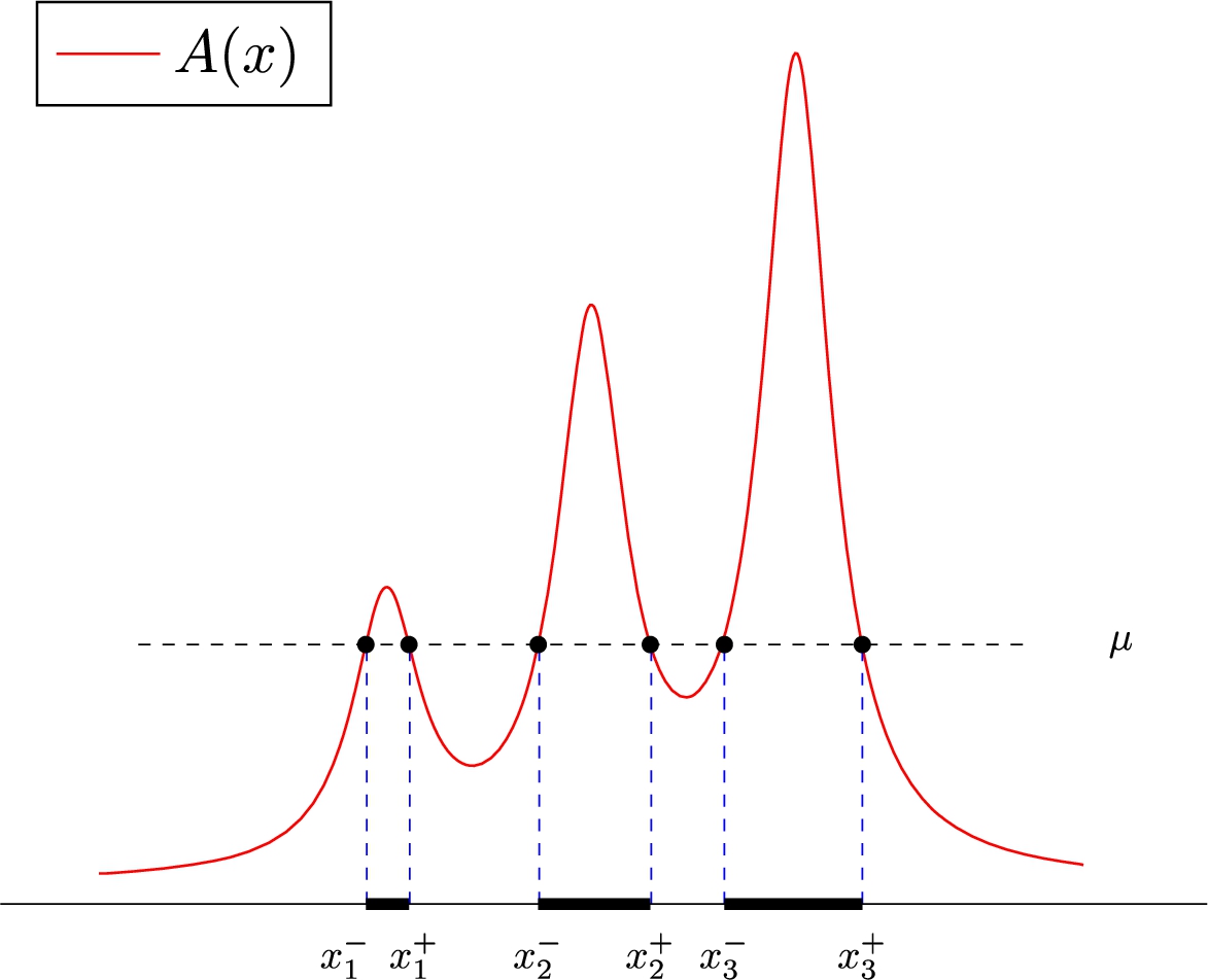
The function $A : R \to R$ is positive, of class $C^{4} (R)$ and such that ${lim}_{x \to \pm \infty} A (x) = 0$ . It has finitely many local extrema and a maximum denoted by $A_{max}$ . Furthermore, in some neighborhoods of these extrema it is of class $C^{5}$ . Additionally, at these extreme points $A^{'}$ vanishes, while $A^{″}$ is either positive (leading to local minima) or negative (for local maxima and maximum). Also, for $μ > 0$ , equation $A (x) = μ$ has only finitely many solutions. Finally, there exists a number $τ > 0$ such that as $| x | \to + \infty$ we have $\begin{array}{c} A (x) = O (\frac{1}{| x |^{1 + τ}}) \\ A^{'} (x) = O (\frac{1}{| x |^{2 + τ}}) \\ A^{″} (x) = O (\frac{1}{| x |^{3 + τ}}) . \end{array}$

4.1. Notation

Fig. 7.

An example of a multi-humped potential.

We begin by fixing some notation. The zeros of equation $A (x) = μ$ for $μ > 0$ can either be simple or double (when they hit an extreme point). Let us first deal with the (non-critical) case where all the zeros of this equation are simple. In such a case, there is a number $L \in N$ so that we can set $x_{ℓ}^{\pm} = x_{ℓ}^{\pm} (μ)$ , $ℓ = 1, \dots, L$ , for these solutions. We enumerate them as follows (see Fig. 7) $\begin{matrix} x_{1}^{-} < x_{1}^{+} < x_{2}^{-} < x_{2}^{+} < \dots < x_{L}^{-} < x_{L}^{+} . \end{matrix}$ Obviously, the number L counts the number of finite barriers that are present. Hence, this yields L barriers $B_{ℓ} (μ) = (x_{ℓ}^{-} (μ), x_{ℓ}^{+} (μ))$ , $ℓ = 1, \dots, L$ of finite width (finite barriers) separated by $L - 1$ wells $W_{ℓ} (μ) = (x_{ℓ}^{+} (μ), x_{ℓ + 1}^{-} (μ))$ , $ℓ = 1, \dots, L - 1$ of finite width (finite wells). We also have two infinite wells (i.e. wells of infinite width) $W_{0} (μ) = (- \infty, x_{1}^{-} (μ))$ and $W_{L} (μ) = (x_{L}^{+} (μ), + \infty)$ . Observe that $\pm A^{'} (x_{ℓ}^{\pm} (μ)) < 0$ for all $ℓ = 1, \dots, L$ . Also, let $b_{ℓ}^{0} (μ) \in B_{ℓ} (μ)$ , $ℓ = 1, \dots, L$ and $w_{ℓ}^{0} (μ) \in W_{ℓ} (μ)$ , $ℓ = 1, \dots, L - 1$ denote the points where A has its extremes.

Using this notation, we define for $ℓ = 1, \dots, L$ the intervals $\begin{matrix} I_{ℓ}^{-} = (x_{ℓ}^{-} (μ), b_{ℓ}^{0} (μ)) and I_{ℓ}^{+} = (b_{ℓ}^{0} (μ), x_{ℓ}^{+} (μ)) \end{matrix}$ and for $ℓ = 1, \dots, L - 1$ the intervals $\begin{matrix} J_{ℓ}^{-} = (x_{ℓ}^{+} (μ), w_{ℓ}^{0} (μ)) and J_{ℓ}^{+} = (w_{ℓ}^{0} (μ), x_{ℓ + 1}^{-} (μ)) \end{matrix}$ Having done this, we define for $ℓ = 1, \dots, L$ the functions $\begin{matrix} F_{ℓ}^{\pm} = {(A |_{clos (I_{ℓ}^{\pm})})}^{- 1} \end{matrix}$ and for $ℓ = 1, \dots, L - 1$ the functions $\begin{matrix} G_{ℓ}^{\pm} = {(A |_{clos (J_{ℓ}^{\pm})})}^{- 1} . \end{matrix}$

Lastly, for each such barrier, we introduce the function $\begin{matrix} (4.1) & Φ_{ℓ} (μ) = \int_{x_{ℓ}^{-} (μ)}^{x_{ℓ}^{+} (μ)} \sqrt{A {(t)}^{2} - μ^{2}} d t . \end{matrix}$ It is easy to check that $Φ_{ℓ}$ is $C^{1}$ . Moreover, differentiating (4.1) and using the relations $A (x_{ℓ}^{\pm}) = μ$ , we obtain $\begin{matrix} (4.2) & \frac{d Φ_{ℓ}}{d μ} (μ) = - 2 μ \int_{x_{ℓ}^{-} (μ)}^{x_{ℓ}^{+} (μ)} {[A {(t)}^{2} - μ^{2}]}^{- 1 / 2} d t < 0 . \end{matrix}$ Thus, $Φ_{ℓ}$ is a one-to-one mapping.

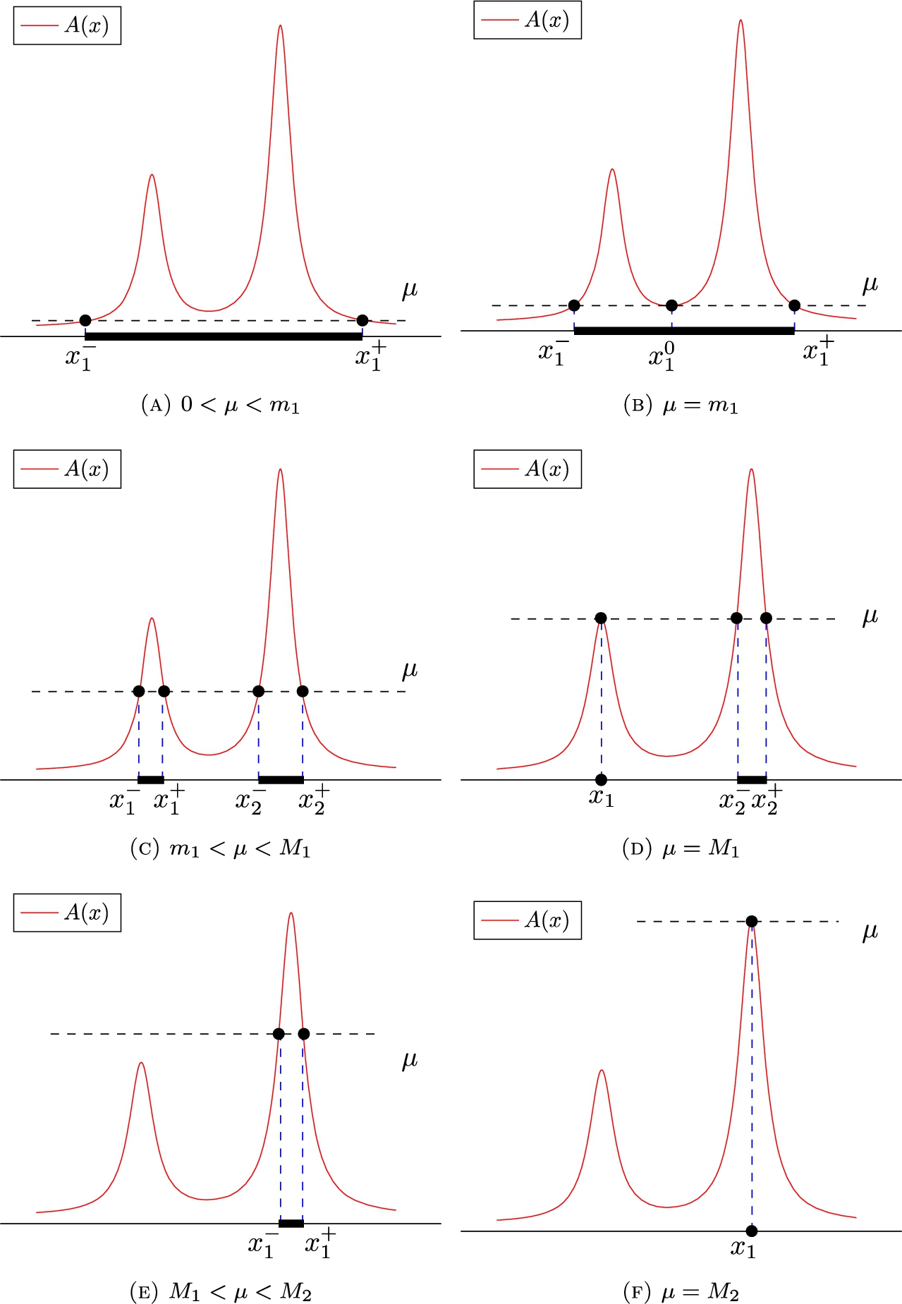
Let us now pass to the case of double zeros. In such a case, we hit local minima and/or local maxima. Without any loss of generality and for clarity and simplicity of notation, we shall deal with the case of a potential function with two humps presented in Fig. 8. In this situation we have a potential A that attains a single local minimum $m_{1}$ and two local maxima $M_{1} < M_{2}$ , the largest of which is the total maximum. Let us examine in detail the two (critical) situations of hitting either a local minimum or a local maximum.

Hitting a local minimum

When $0 < μ < m_{1}$ (cf. Fig. 8a) we have only one finite barrier $(x_{1}^{-} (μ), x_{1}^{+} (μ))$ . When μ grows to reach $m_{1}$ , equation $A (x) = m_{1}$ has now three zeros; two simple at $x_{1}^{\pm} (m_{1})$ and one double at $x_{1}^{0} (m_{1})$ (see Fig. 8b). Observe that in such a case, there emerges a new point $x_{1}^{0}$ between $x_{1}^{-} < x_{1}^{+}$ that previously (i.e. when $μ < m_{1}$ ) defined the barrier. This new point will give rise to a new well and the barrier will split into two barriers.

Hitting a local maximum

When $M_{1} < μ < M_{2}$ (cf. Fig. 8e) we see that we again have only one finite barrier $(x_{1}^{-} (μ), x_{1}^{+} (μ))$ . When μ grows to reach $M_{2}$ , equation $A (x) = M_{2}$ has now only one zero; a double one at $x_{1}$ . (see Fig. 8f). Observe that in such a case, the two points that previously (i.e. when $M_{1} < μ < M_{2}$ ) defined a barrier coalesce to a single point $x_{1}$ . The same behavior is observed in Figs 8c and 8d when $μ = M_{1}$ . In this latter case we are left with a double zero $x_{1} (M_{1})$ and a finite barrier having as endpoints the simple zeros $x_{2}^{-} (M_{1})$ and $x_{2}^{+} (M_{1})$ .

The general case follows exactly by arguing along the same lines of the observations just made. In short, when we hit a local minimum, a new well is being created inside a barrier, while when we hit a local maximum, a barrier is reduced to a point.

Fig. 8.

The case of a potential function A with two humps. In each subfigure, the “energy” (spectral parameter) μ takes on different values in $R_{A}$ .

4.2. Statement of the problem

We study the problem $\begin{matrix} (4.3) & D_{ℏ} [u] = λ u \end{matrix}$ where $D_{ℏ}$ is the following Dirac (or Zakharov–Shabat) operator $\begin{matrix} (4.4) & D_{ℏ} = [\begin{array}{cc} i ℏ \partial_{x} & - i A \\ - i A & - i ℏ \partial_{x} \end{array}] \end{matrix}$ with ℏ a positive parameter, A a function satisfying Assumption 4.1 and $u = {[u_{1} u_{2}]}^{T}$ a function from $R$ to $C^{2}$ . As usual, $λ \in C$ plays the role of the spectral parameter.

Definition 4.2.
For a fixed $ℏ > 0$ , we say that $λ \in C$ is an eigenvalue (EV) of the densely defind operator $D_{ℏ}$ (4.4) on $L^{2} (R; C^{2})$ , if equation (4.3) -with this value of λ- has a non-trivial solution $u = {[u_{1} u_{2}]}^{T} \in L^{2} (R; C^{2})$ ; that is $\begin{matrix} 0 < \int_{- \infty}^{+ \infty} [{| u_{1} (x) |}^{2} + {| u_{2} (x) |}^{2}] d x < + \infty . \end{matrix}$

In general, a non-self-adjoint operator like $D_{ℏ}$ has complex EVs. For such an operator (with a potential A satisfying Assumption 4.1), we know the following about its spectrum (see article [13] by Klaus and Shaw and [10] by Hirota and Wittsten).
If $D_{ℏ}$ has EVs, then there is a purely imaginary EV whose imaginary part is strictly larger than the imaginary part of any other EV.

The EV formation threshold is $\begin{matrix} ℏ^{- 1} ‖ A ‖_{L^{1} (R)} > \frac{π}{2} \end{matrix}$ and is hence always achieved for sufficiently small ℏ.

Let N be the largest nonnegative integer such that $\begin{matrix} ℏ^{- 1} ‖ A ‖_{L^{1} (R)} > (2 N - 1) \frac{π}{2} . \end{matrix}$ Then there are at least N purely imaginary EVs.

The spectrum of $D_{ℏ}$ is symmetric with respect to reflection in $R$ .

The continuous (essential) spectrum consists of the entire real line $R$ , i.e. $\begin{matrix} σ_{ess} (D_{ℏ}) = R . \end{matrix}$
The following assumption will make our analysis easier. We assume that for sufficiently small $ℏ > 0$ , $D_{ℏ}$ has only purely imaginary EVs.
Assumption 4.3.
For the point spectrum of $D_{ℏ}$ we suppose that $\begin{matrix} \exists ℏ_{0} > 0 such that \forall ℏ \in (0, ℏ_{0}) we have σ_{p} (D_{ℏ}) \subset i [- A_{max}, A_{max}] . \end{matrix}$

We will show later that this assumption is not strictly necessary (and in fact it is shown a posteriori to be true for all smooth potentials A satisfying Assumption 4.1; see appendix A). But for the moment we simply take it for granted since it makes the straightforward application of Olver’s theory possible. Hence, from now on we always assume that $0 < ℏ < ℏ_{0}$ .
4.3. Trasforming spectral parameter & changing variables

From now on we assume that the Assumption 4.3 is satisfied. Recall also that the spectrum of $D_{ℏ}$ is symmetric with respect to reflection in $R$ . Hence, we consider the spectral parameter $λ \in i (0, A_{max}]$ and change it to a real $μ \in R_{+}$ by setting $\begin{matrix} (4.5) & λ = i μ . \end{matrix}$ Hence, (4.3) is written as $\begin{matrix} (4.6) & ℏ [\begin{array}{c} u_{1}^{'} (x, μ, ℏ) \\ u_{2}^{'} (x, μ, ℏ) \end{array}] = [\begin{array}{cc} μ & A (x) \\ - A (x) & - μ \end{array}] [\begin{array}{c} u_{1} (x, μ, ℏ) \\ u_{2} (x, μ, ℏ) \end{array}], x \in R . \end{matrix}$

Under the change of variables (cf. equation (4) in [14]) $\begin{matrix} (4.7) & y_{\pm} = \frac{u_{2} \pm u_{1}}{\sqrt{A \mp μ}} \end{matrix}$ system (4.6) is equivalent to the following two independent eigenvalue equations $\begin{matrix} (4.8) & y_{\pm}^{″} (x, μ, ℏ) = {ℏ^{- 2} [μ^{2} - A^{2} (x)] + \frac{3}{4} {[\frac{A^{'} (x)}{A (x) \mp μ}]}^{2} - \frac{1}{2} \frac{A^{″} (x)}{A (x) \mp μ}} y_{\pm} (x, μ, ℏ), x \in R . \end{matrix}$

Since $A (x) \in R_{+}$ , $x \in R$ , we will only consider the “minus” case for the lower index in (4.8) and thus work with the equation $\begin{matrix} (4.9) & \frac{d^{2} y}{d x^{2}} = {ℏ^{- 2} [μ^{2} - A^{2} (x)] + \frac{3}{4} {[\frac{A^{'} (x)}{A (x) + μ}]}^{2} - \frac{1}{2} \frac{A^{″} (x)}{A (x) + μ}} y, x \in R . \end{matrix}$

Observe that the change of variables (4.7) does not alter the discrete spectrum. So we have arrived at the following proposition.

Proposition 4.4.
Under Assumptions 4.1 and 4.3 , finding the discrete spectrum of $D_{ℏ}$ in ( 4.4 ), is equivalent to finding the values $μ \in (0, A_{max}]$ for which ( 4.9 ) has an $L^{2} (R; C)$ solution.

4.4. Reformulating the equation

In a neighborhood of a finite (noncritical) barrier $B_{ℓ} = (x_{ℓ}^{-}, x_{ℓ}^{+})$ , $ℓ = 1, \dots, L$ , equation (4.9) can be written as $\begin{matrix} \frac{d^{2} y}{d x^{2}} = [ℏ^{- 2} f (x, x_{ℓ}^{+}) + g (x, x_{ℓ}^{+})] y \end{matrix}$ where f and g satisfy $\begin{matrix} f (x, x_{ℓ}^{+}) = A^{2} (x_{ℓ}^{+}) - A^{2} (x) \end{matrix}$ and $\begin{matrix} g (x, x_{ℓ}^{+}) = \frac{3}{4} {[\frac{A^{'} (x)}{A (x) + A (x_{ℓ}^{+})}]}^{2} - \frac{1}{2} \frac{A^{″} (x)}{A (x) + A (x_{ℓ}^{+})} . \end{matrix}$ This means that in a neighborhood of a barrier we can use the results obtained in §2.

Similarly, in a neighborhood of a finite (noncritical) well $W_{ℓ} = (x_{ℓ}^{+}, x_{ℓ + 1}^{-})$ , $ℓ = 1, \dots, L - 1$ , equation (4.9) can be put in the form $\begin{matrix} \frac{d^{2} y}{d x^{2}} = [ℏ^{- 2} f (x, x_{ℓ}^{+}) + g (x, x_{ℓ}^{+})] y \end{matrix}$ where f and g satisfy $\begin{matrix} f (x, x_{ℓ}^{+}) = A^{2} (x_{ℓ}^{+}) - A^{2} (x) \end{matrix}$ and $\begin{matrix} g (x, x_{ℓ}^{+}) = \frac{3}{4} {[\frac{A^{'} (x)}{A (x) + A (x_{ℓ}^{+})}]}^{2} - \frac{1}{2} \frac{A^{″} (x)}{A (x) + A (x_{ℓ}^{+})} . \end{matrix}$ This guarantees that in a neighborhood of a well we can use the results of §3.

From paragraphs §2 and §3 we know that after applying the Liouville transform, the above differential equations are transformed correspondingly to the form $\begin{matrix} (4.10) & \frac{d^{2} X}{d ζ^{2}} = [\pm ℏ^{- 2} (ζ^{2} - γ^{2}) + φ (ζ, γ)] X \end{matrix}$ where for the “+” sign, $γ = α$ and $φ = ψ$ (cf. §2.1) while for the “−” case, $γ = β$ and $φ = \overline{ψ}$ (see §3.1). Keeping in mind Proposition 4.4 we are led to the following.

Proposition 4.5.
Under Assumptions 4.1 and 4.3 , finding the discrete spectrum of $D_{ℏ}$ in ( 4.4 ) is equivalent to finding the values $α ⩾ 0$ for which equation ( 4.10 ), for the “+” sign with $γ = α$ , $φ = ψ$ , has an $L^{2} (R; C)$ solution.

5. Semiclassical spectral results for multiple barriers

In this section, we use the results from paragraphs §2 and §3 to study the EVs and their corresponding norming constants of a Dirac operator with potential A. Here, we let this potential have multiple humps (see Fig. 7). To be precise, we assume the following.

5.1. Quantization conditions for the EVs

In this subsection, using Assumptions 4.1, 4.3 and what we have gathered so far, we present the results for the EVs of the Dirac operator $D_{ℏ}$ .

Theorem 5.1.
Consider a potential A of the Dirac operator $D_{ℏ}$ in ( 4.4 ) that satisfies Assumption 4.1 . Also assume Assumption 4.3 and take $0 < μ_{1} < μ_{2} ⩽ A_{max}$ . Suppose that $λ = i μ \in i [μ_{1}, μ_{2}]$ (where $λ = λ (ℏ)$ and $μ = μ (ℏ)$ ) is an EV of $D_{ℏ}$ . Then using the notation from § 4.1 , at least for one $ℓ = ℓ (ℏ) \in {1, 2, \dots, L}$ , there is a non-negative integer $n = n (μ, ℓ, ℏ)$ such that $\begin{matrix} (5.1) & Φ_{ℓ} (μ) = π (n + \frac{1}{2}) ℏ + O (ℏ^{\frac{5}{3}}) as ℏ ↓ 0 . \end{matrix}$
Proof.
From Theorem 3.16 we see that each well $W_{ℓ} (μ)$ , $ℓ = 1, \dots, L - 1$ yields at least one fixing condition (cf. (3.41)). Moreover, the asymptotic form of $Y_{+} (ζ, α (μ), ℏ)$ as $ζ \to + \infty$ and the asymptotics for $Y_{-} (ζ, α (μ), ℏ)$ and $Z_{-} (ζ, α (μ), ℏ)$ as $ζ \to - \infty$ (see (2.23), (2.30) and (2.31)) show that in the presense of an EV, the coefficient $σ_{12}$ in equation (2.32) has to be zero. But this is translated to the fact that the fixing conditions are fulfilled at the right point $x_{1}^{-} (μ)$ of the well $W_{0} (μ)$ and at the left point $x_{L}^{+} (μ)$ of the well $W_{L} (μ)$ . Thus for every $0 < ℏ < ℏ_{0}$ , we have at least $L + 1$ fixing conditions for L barriers. Hence, there exists a barrier $B_{ℓ} (μ, ℏ)$ (depending on ℏ as well) for which a fixing condition is satisfied on each of its two ends. Finally, we refer to Theorem 2.19 which gives us the desired results. □

Formula (4.2) implies $Φ_{ℓ}$ is a one-to-one mapping, so there exists an inverse $Φ_{ℓ}^{- 1}$ and we can write (5.1) equivalently as $\begin{matrix} (5.2) & μ (ℏ) = Φ_{ℓ}^{- 1} [π (n + \frac{1}{2}) ℏ] + O (ℏ^{\frac{5}{3}}) as ℏ ↓ 0 . \end{matrix}$ This formula (5.2) leads to the following definition of WKB EVs.
Definition 5.2.
We call the numbers $\begin{matrix} (5.3) & λ_{ℓ, n}^{WKB} (ℏ) = i μ_{ℓ, n}^{WKB} (ℏ) = i Φ_{ℓ}^{- 1} [π (n + \frac{1}{2}) ℏ] \end{matrix}$ WKB eigenvalues.

If $λ (ℏ) = i μ (ℏ)$ is an EV of $D_{ℏ}$ , then from Theorem 5.1 there exists at least one $ℓ \in {1, 2, \dots, L}$ so that $λ_{ℓ, n}^{WKB} (ℏ)$ is close to $λ (ℏ)$ for some $n \in N$ .

Consider now the intervals $\begin{matrix} (5.4) & Δ_{ℓ, n} (ℏ) = (μ_{ℓ, n}^{WKB} (ℏ) - c ℏ^{\frac{5}{3}}, μ_{ℓ, n}^{WKB} (ℏ) + C ℏ^{\frac{5}{3}}) \end{matrix}$ for some arbitrary ℏ-independent constants $c, C > 0$ . The lengths of these intervals are of order $O (ℏ^{\frac{5}{3}})$ while for different $m, n \in N$ the distances between the points $μ_{ℓ, m}^{WKB} (ℏ)$ and $μ_{ℓ, n}^{WKB} (ℏ)$ are of order $O (ℏ)$ . This says that for sufficiently small ℏ $\begin{matrix} Δ_{ℓ, m} (ℏ) \cap Δ_{ℓ, n} (ℏ) = \emptyset for m \neq n . \end{matrix}$ However if we consider different $k, ℓ \in {1, 2, \dots, L}$ , it may occur that $\begin{matrix} Δ_{k, n} (ℏ) \cap Δ_{ℓ, n} (ℏ) \neq \emptyset for k \neq ℓ . \end{matrix}$

Theorem (5.1) says that each EV of $D_{ℏ}$ belongs to one of the intervals $i Δ_{ℓ, n} (ℏ)$ . Hence for sufficiently small ℏ, equivalently stated this can be written as $\begin{matrix} σ_{p} (D_{ℏ}) \cap i (μ_{1}, μ_{2}) \subset ⋃_{ℓ = 1}^{L} ⋃_{n} i Δ_{ℓ, n} (ℏ) \end{matrix}$ or $\begin{matrix} dist {σ_{p} (D_{ℏ}) \cap i (μ_{1}, μ_{2}), ⋃_{ℓ = 1}^{L} ⋃_{n \in N} {λ_{ℓ, n}^{WKB} (ℏ) | n \in N}} = O (ℏ^{\frac{5}{3}}) as ℏ ↓ 0 . \end{matrix}$

Conversely for the existence of an actual EV for our operator in (4.4), we have the following theorem.
Theorem 5.3.
Let Assumption 4.1 be satisfied by A and assume Assumption 4.3 for $D_{ℏ}$ . Then for every $ℓ \in {1, 2, \dots, L}$ and every non-negative integer n such that $\begin{matrix} (5.5) & Φ_{ℓ}^{- 1} [π (n + \frac{1}{2}) ℏ] \in (μ_{1}, A_{max}) \end{matrix}$ there exists an EV of $D_{ℏ}$ , namely $λ = i μ$ (where $λ = λ (ℓ, n, ℏ)$ and $μ = μ (ℓ, n, ℏ)$ ), that satisfies $\begin{matrix} λ = λ_{ℓ, n}^{WKB} (ℏ) + O (ℏ^{\frac{5}{3}}) as ℏ ↓ 0 . \end{matrix}$ Furthermore the associated norming constants have asymptotics ${(- 1)}^{n} + O (ℏ^{\frac{2}{3}})$ .
Proof.
Fix some $ℓ \in {1, 2, \dots, L}$ and some non-negative integer n so that (5.5) is true. By Theorem 2.21, there exists $μ = μ (ℓ, n, ℏ)$ such that $\begin{matrix} (5.6) & μ = Φ_{ℓ}^{- 1} [π (n + \frac{1}{2}) ℏ] + O (ℏ^{\frac{5}{3}}) as ℏ ↓ 0 \end{matrix}$ and such that $\begin{matrix} Y_{-} (ζ, α_{ℓ} (μ), ℏ) = σ (α_{ℓ} (μ), ℏ) Y_{+} (ζ, α_{ℓ} (μ), ℏ) \end{matrix}$ where $\begin{matrix} (5.7) & α_{ℓ} (μ) = \sqrt{\frac{2}{π} Φ_{ℓ} (μ)} and σ (α_{ℓ} (μ), ℏ) = {(- 1)}^{n} + O (ℏ^{\frac{2}{3}}) as ℏ ↓ 0 . 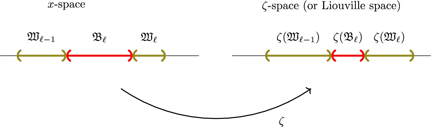\end{matrix}$ Fixing this value of μ, let a cut-off function $χ_{ℓ} \in C_{0}^{\infty} (R)$ be such that $χ_{ℓ} (ζ) = 1$ in some neighborhood of the interval $ζ (B_{ℓ} (μ))$ (recall that ζ is a continuous and increasing function of x) and $χ_{ℓ} (ζ) = 0$ outside of some larger neighborhood of that interval. In particularly, we have $χ_{ℓ} (ζ) = 0$ on all other intervals $ζ (B_{k} (μ))$ with $k \neq ℓ$ . We set $\begin{matrix} f_{ℓ, n} (ζ, ℏ) = Y_{-} (ζ, α_{ℓ} (μ), ℏ) χ_{ℓ} (ζ) . \end{matrix}$ Observe that $f_{ℓ, n} (\cdot, ℏ) \in C_{0}^{2} (R)$ . Since the function $Y_{-} (ζ, α_{ℓ} (μ), ℏ)$ satisfies $\begin{matrix} \frac{d^{2} Y_{-}}{d ζ^{2}} = [ℏ^{- 2} (ζ^{2} - α_{ℓ}^{2} (μ)) + ψ (ζ, α_{ℓ} (μ))] Y_{-} \end{matrix}$ for $f_{ℓ, n}$ we have $\begin{array}{c} \frac{d^{2} f_{ℓ, n}}{d ζ^{2}} - [ℏ^{- 2} (ζ^{2} - α_{ℓ}^{2} (\tilde{μ})) + ψ (ζ, α_{ℓ} (μ))] f_{ℓ, n} \\ = 2 \frac{d Y_{-}}{d ζ} \frac{d χ_{ℓ}}{d ζ} + Y_{-} \frac{d^{2} χ_{ℓ}}{d ζ^{2}} \\ = σ (α_{ℓ} (μ), ℏ) (2 \frac{d Y_{+}}{d ζ} \frac{d χ_{ℓ}}{d ζ} + Y_{+} \frac{d^{2} χ_{ℓ}}{d ζ^{2}}) . \end{array}$

Fig. 9.
Barriers and wells in x-space and Liouville space.

Due to the derivatives of $χ_{ℓ}$ , the expression above differs from zero only on compact subsets of the intervals $ζ (W_{ℓ - 1} (μ))$ and $ζ (W_{ℓ} (μ))$ (see Fig. 9). But the definitions of $Y_{\pm}$ and σ along with (D.2) show that this expression tends to zero as $ℏ ↓ 0$ on both $ζ (W_{ℓ - 1} (μ))$ and $ζ (W_{ℓ} (μ))$ . This shows (cf. Proposition 4.5) that $λ = i μ$ is the desired EV. Finally, using the definition (5.3) and (5.6) we find that λ satisfies the specified asymptotics as $ℏ ↓ 0$ . The asymptotics for the norming constants follow from (5.7). □
Remark 5.4.
We cannot exclude the possibility that EVs coming from different barriers (i.e. different values of ℓ) get too close (at a distance of order $o (ℏ^{5 / 3})$ ) or even coincide. So we could even have double EVs. But this does not affect the applications to NLS. For the semiclassical analysis of the inverse scattering, the important fact is that we have different sets of EVs from different barriers, each set with a different density (see Appendix B below).
5.2. Eigenvalues near zero and their corresponding norming constants

For the applications to the semiclassical theory of the focusing NLS equation, it is important to understand the behavior of the EVs near 0. The problem is essentially the same as the one we considered in [9]. We can actually improve our result somewhat and we present the details here.

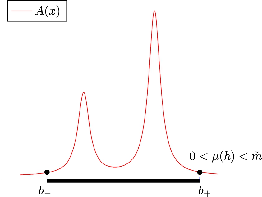
We begin with a potential function A that satisfies Assumption 4.1. Such a function has finitely many local minima, say $N \in N_{0}$ , accounting for the case of a function having none ( $N = 0$ ); if there are $N \in N$ local minima, we denote them by $m_{j}$ , $j = 1, \dots, N$ . We set $\tilde{m}$ to be $\begin{matrix} (5.8) & \tilde{m} = \{\begin{array}{ll} A_{max}, & if N = 0 \\ {min}_{j \in {1, \dots, N}} m_{j}, & if N \in N . \end{array} \end{matrix}$ In this section we investigate the (semiclassical) behavior of EVs of $D_{ℏ}$ (with potential A) that lie in $i (0, \tilde{m})$ , so that $μ (ℏ) \in (0, \tilde{m})$ and also $μ (ℏ) ↓ 0$ as $ℏ ↓ 0$ . We emphasize that we are in the presence of only one (finite) barrier (see Fig. 10). So $l = 1$ . In this setting, using (2.4), (2.5), (2.20) and having in mind that $A (b_{\pm}) = μ$ (for the notation, consult §2.1), we define $\begin{array}{c} (5.9) & \bar{f} (x, ℏ) = f (x, b_{+} (μ (ℏ))) = μ {(ℏ)}^{2} - A^{2} (x) \\ (5.10) & \bar{g} (x, ℏ) = g (x, b_{+} (μ (ℏ))) = \frac{3}{4} {[\frac{A^{'} (x)}{A (x) + μ (ℏ)}]}^{2} - \frac{1}{2} \frac{A^{″} (x)}{A (x) + μ (ℏ)} \end{array}$ and $\begin{matrix} \bar{f} (x, ℏ) = (x - b_{-} (μ (ℏ))) (x - b_{+} (μ (ℏ))) \bar{p} (x, ℏ) . \end{matrix}$ where $\begin{matrix} \bar{p} (x, ℏ) = p (x, b_{+} (μ (ℏ))) . \end{matrix}$

Fig. 10.

The potential barrier in a case of near zero EVs.

We apply the Liouville transform once again (as in §2.1), and arrive at the following proposition (cf. Proposition 2.7).

Proposition 5.5.

For every $ℏ > 0$ , equation $\begin{matrix} \frac{d^{2} y}{d x^{2}} = [ℏ^{- 2} \bar{f} (x, ℏ) + \bar{g} (x, ℏ)] y, x \in R \end{matrix}$ is transformed to equation $\begin{matrix} \frac{d^{2} X}{d ζ^{2}} = [ℏ^{- 2} (ζ^{2} - α {(μ (ℏ))}^{2}) + ψ (ζ, α (μ (ℏ)))] X, ζ \in R \end{matrix}$ in which ζ is given by the Liouville transform ( 2.7 ), α is given by ( 2.9 ) and the function $ψ (ζ, α (μ (ℏ)))$ is given by the formula $\begin{array}{rcl} ψ (ζ, α (μ (ℏ))) & = & \frac{1}{4} \frac{3 ζ^{2} + 2 α {(μ (ℏ))}^{2}}{{[ζ^{2} - α {(μ (ℏ))}^{2}]}^{2}} + \frac{1}{16} \frac{ζ^{2} - α {(μ (ℏ))}^{2}}{\bar{f} {(x, ℏ)}^{3}} \\ \cdot [4 \bar{f} (x, ℏ) {\bar{f}}^{″} (x, ℏ) - 5 {\bar{f}}^{'} {(x, ℏ)}^{2}] + [ζ^{2} - α {(μ (ℏ))}^{2}] \frac{\bar{g} (x, ℏ)}{\bar{f} (x, ℏ)} \end{array}$ where prime denotes differentiation with respect to x.

Remark 5.6.

By recalling the definition of α in (2.9), and the fact that $b_{\pm} (μ (ℏ)) \to \pm \infty$ , as $ℏ ↓ 0$ , we obtain $\begin{matrix} (5.11) & α (μ (ℏ)) ↑ \sqrt{\frac{2}{π} ‖ A ‖_{L^{1} (R)}} as ℏ ↓ 0 . \end{matrix}$

It is easy to see that for each value of ℏ, the functions $\bar{f}$ , $\bar{g}$ and $\bar{p}$ satisfy properties (i) through (iv) in the proof of Lemma 2.10 in §2.2. This in turn implies -again with the help of Lemma I in [16]- that for each ℏ the function $\begin{array}{rcl} ψ (ζ, α (μ (ℏ))) & = & \frac{1}{4} \frac{3 ζ^{2} + 2 α {(μ (ℏ))}^{2}}{{[ζ^{2} - α {(μ (ℏ))}^{2}]}^{2}} + \frac{1}{16} \frac{ζ^{2} - α {(μ (ℏ))}^{2}}{\bar{f} {(x, ℏ)}^{3}} \\ (5.12) & \cdot [4 \bar{f} (x, ℏ) {\bar{f}}^{″} (x, ℏ) - 5 {\bar{f}}^{'} {(x, ℏ)}^{2}] + [ζ^{2} - α {(μ (ℏ))}^{2}] \frac{\bar{g} (x, ℏ)}{\bar{f} (x, ℏ)} \end{array}$ is continuous in the corresponding region of the $(ζ, α)$ -plane.

So in order to have a conclusion such as Theorem 2.13 and eventually results like Theorem 2.19 and Theorem 2.21, we need to investigate the convergence of the integral in (2.27) (cf. proof of Theorem 2.13 or proof of Theorem 6.3 in §6 of [9]), i.e. $\begin{matrix} (5.13) & \int_{0}^{+ \infty} \frac{| ψ (t, α (μ (ℏ))) |}{Ω (t \sqrt{2 ℏ^{- 1}})} d t . \end{matrix}$

Here we need to place an additional assumption on the behavior of the potential A at $\pm \infty$ .

Assumption 5.7.

Suppose there are real positive numbers $1 < r_{+} ⩽ s_{+}$ , so that $\begin{matrix} \frac{C_{1}^{+} (x)}{| x |^{s_{+}}} ⩽ A (x) ⩽ \frac{C_{2}^{+} (x)}{| x |^{r_{+}}} for x > 0 \end{matrix}$ where $C_{1}^{+}$ , $C_{2}^{+}$ are bounded functions and $2 r_{+} - s_{+} > \frac{1}{3}$ ; and there are real positive numbers $1 < r_{-} ⩽ s_{-}$ , so that $\begin{matrix} \frac{C_{1}^{-} (x)}{| x |^{s_{-}}} ⩽ A (x) ⩽ \frac{C_{2}^{-} (x)}{| x |^{r_{-}}} for x < 0 \end{matrix}$ where $C_{1}^{-}$ , $C_{2}^{-}$ are bounded functions and $2 r_{-} - s_{-} > \frac{1}{3}$ . Alternatively, suppose there are real positive numbers $0 < r ⩽ s$ so that $\begin{matrix} C_{1} (x) e^{- | x |^{s}} ⩽ A (x) ⩽ C_{2} (x) e^{- | x |^{r}}, x \in R \end{matrix}$ where $C_{1}$ , $C_{2}$ are bounded functions.

Finally, recall (2.13) where now $x_{2} = + \infty$ . It shows that $x ↑ + \infty$ as $ζ ↑ + \infty$ . The lemma below deals with the asymptotic behavior of x as $ζ ↑ + \infty$ . It shall be used to allow us understand the nature of ψ for large ζ.

Lemma 5.8.

Considering x as a function of ζ we see that $\begin{matrix} (5.14) & x = \frac{ζ^{2}}{2 μ} [1 + O (\frac{log ζ}{ζ^{2}})] as ζ ↑ + \infty \end{matrix}$ uniformly with respect to $μ = A (b_{\pm}) \in (0, \tilde{m})$ .

Proof.

See Lemma 5.2 in §5 of [9]. □

It is now straightforward to check that Olver’s theory is uniformly applicable all the way to $μ = 0$ . For example, consider first the case where A is rational: $\begin{matrix} (5.15) & A (x) = \frac{1}{| x |^{r}} for | x | ⩾ 1 \end{matrix}$ where $r > 1$ (clearly satisfying Assumption 2.4 and Assumption 5.7). In this case, using (5.14) we get $\begin{matrix} (5.16) & x = \frac{ζ^{2}}{2 μ (ℏ)} [1 + O (\frac{log ζ}{ζ^{2}})] as ζ ↑ + \infty \end{matrix}$ while using (5.9), (5.10), (5.12), (5.15) and (5.16) we arrive at $\begin{matrix} (5.17) & ψ (ζ, α (μ (ℏ))) = ψ_{1} (ζ, α (μ (ℏ))) [1 + O (\frac{log ζ}{ζ^{2}})] as ζ ↑ + \infty \end{matrix}$ uniformly in α and consequently in ℏ, where $\begin{aligned} ψ_{1} (ζ, α (μ (ℏ))) & = \frac{1}{4} \frac{3 ζ^{2} + 2 α {(μ (ℏ))}^{2}}{{[ζ^{2} - α {(μ (ℏ))}^{2}]}^{2}} \\ - r (2 r + 1) 2^{2 r + 1} μ {(ℏ)}^{2 r - 2} ζ^{4 r - 4} [ζ^{2} - α {(μ (ℏ))}^{2}] \\ \cdot \frac{ζ^{4 r} + \frac{r - 2}{2 r + 1} 2^{2 r - 1} μ {(ℏ)}^{2 r - 2}}{{[ζ^{4 r} - 2^{2 r} μ {(ℏ)}^{2 r - 2}]}^{3}} \\ - r (r + 1) 2^{r + 1} μ {(ℏ)}^{r - 1} ζ^{4 r - 4} [ζ^{2} - α {(μ (ℏ))}^{2}] \\ \cdot \frac{ζ^{2 r} - \frac{r - 2}{r + 1} 2^{r - 1} μ {(ℏ)}^{r - 1}}{[ζ^{2 r} - 2^{r} μ {(ℏ)}^{r - 1}] {[ζ^{2 r} + 2^{r} μ {(ℏ)}^{r - 1}]}^{3}} . \end{aligned}$

Consider now the case where A is exponentially decreasing: $\begin{matrix} (5.18) & A (x) = e^{- | x |^{r}} for | x | ⩾ 1 \end{matrix}$ where $r > 0$ ; it clearly satisfies Assumption 2.4 and Assumption 5.7). Using (5.9), (5.10), (5.12), (5.14), (5.15) and (5.16) we arrive at $\begin{matrix} (5.19) & ψ (ζ, α (μ (ℏ))) = ψ_{2} (ζ, α (μ (ℏ))) [1 + O (\frac{log ζ}{ζ^{2}})] as ζ ↑ + \infty \end{matrix}$ uniformly in α and consequently in ℏ, where $\begin{aligned} ψ_{2} (ζ, α (μ (ℏ))) & = \frac{1}{4} \frac{3 ζ^{2} + 2 α {(μ (ℏ))}^{2}}{{[ζ^{2} - α {(μ (ℏ))}^{2}]}^{2}} \\ + \frac{r}{2^{r}} \frac{ζ^{2} - α {(μ (ℏ))}^{2}}{μ {(ℏ)}^{r - 2}} \frac{ζ^{2 r - 4} exp {- \frac{ζ^{2 r}}{2^{r - 1} μ {(ℏ)}^{r}}}}{{[exp {- \frac{ζ^{2 r}}{2^{r - 1} μ {(ℏ)}^{r}}} - μ {(ℏ)}^{2}]}^{3}} \\ \cdot [\frac{r}{2^{r}} \frac{ζ^{2 r}}{μ {(ℏ)}^{r}} exp {- \frac{ζ^{2 r}}{2^{r - 1} μ {(ℏ)}^{r}}} + 2 (r - 1) exp {- \frac{ζ^{2 r}}{2^{r - 1} μ {(ℏ)}^{r}}} \\ + \frac{r}{2^{r - 2}} \frac{ζ^{2 r}}{μ {(ℏ)}^{r - 2}} - 2 (r - 1) μ {(ℏ)}^{2}] \\ - \frac{r}{2^{r - 1}} \frac{ζ^{2} - α {(μ (ℏ))}^{2}}{μ {(ℏ)}^{r - 2}} \frac{ζ^{2 r - 4} exp {- \frac{ζ^{2 r}}{2^{r} μ {(ℏ)}^{r}}}}{[exp {- \frac{ζ^{2 r}}{2^{r} μ {(ℏ)}^{r}}} - μ (ℏ)] {[exp {- \frac{ζ^{2 r}}{2^{r} μ {(ℏ)}^{r}}} + μ (ℏ)]}^{3}} \\ \cdot [\frac{r}{2^{r + 1}} \frac{ζ^{2 r}}{μ {(ℏ)}^{r}} exp {- \frac{ζ^{2 r}}{2^{r} μ {(ℏ)}^{r}}} + (r - 1) exp {- \frac{ζ^{2 r}}{2^{r} μ {(ℏ)}^{r}}} \\ - \frac{r}{2^{r}} \frac{ζ^{2 r}}{μ {(ℏ)}^{r - 1}} + (r - 1) μ (ℏ)] . \end{aligned}$

These asymptotics imply that for each $ℏ > 0$ , the integral in (5.13) converges; furthermore, this convergence is uniform in α. Now similar computations can be easily performed for any A satisfying Assumption 2.4 and Assumption 5.7. One uses the upper bound of Assumption 5.7 for the numerator and the lower bound for the denominator. The result remains the same. The integral in (5.13) converges uniformly in α. A variation of Theorem 2.13 can be applied to guarantee the existence of approximate solutions in these cases too. Hence, we arrive at the following theorem.

Theorem 5.9.

For every $ℏ > 0$ , equation $\begin{matrix} (5.20) & \frac{d^{2} Y}{d ζ^{2}} = [ℏ^{- 2} (ζ^{2} - α {(μ (ℏ))}^{2}) + ψ (ζ, α (μ (ℏ)))] Y \end{matrix}$ has in the region $[0, + \infty) \times [0, α (μ (ℏ))]$ of the $(ζ, α)$ -plane solutions $Y_{+}$ and $Z_{+}$ which are continuous, have continuous first and second partial ζ-derivatives, and are given by $\begin{array}{c} Y_{+} (ζ, α (μ (ℏ)), ℏ) = U (ζ \sqrt{2 ℏ^{- 1}}, - \frac{1}{2} ℏ^{- 1} α {(μ (ℏ))}^{2}) + ε (ζ, α (μ (ℏ)), ℏ) \\ Z_{+} (ζ, α (μ (ℏ)), ℏ) = \overline{U} (ζ \sqrt{2 ℏ^{- 1}}, - \frac{1}{2} ℏ^{- 1} α {(μ (ℏ))}^{2}) + \overline{ε} (ζ, α (μ (ℏ)), ℏ) \end{array}$ (cf. ( 2.23 ), ( 2.24 )) where for the remainders we have the relations $\begin{array}{c} \frac{| ε (ζ, α (μ (ℏ)), ℏ) |}{M (ζ \sqrt{2 ℏ^{- 1}}, - \frac{1}{2} ℏ^{- 1} α {(μ (ℏ))}^{2})}, \frac{| \frac{\partial ε}{\partial ζ} (ζ, α (μ (ℏ)), ℏ) |}{\sqrt{2 ℏ^{- 1}} N (ζ \sqrt{2 ℏ^{- 1}}, - \frac{1}{2} ℏ^{- 1} α {(μ (ℏ))}^{2})} \\ ⩽ \frac{1}{E (ζ \sqrt{2 ℏ^{- 1}}, - \frac{1}{2} ℏ^{- 1} α {(μ (ℏ))}^{2})} \\ \times (exp {\frac{1}{2} {(π ℏ)}^{\frac{1}{2}} l_{1} (- \frac{1}{2} ℏ^{- 1} α {(μ (ℏ))}^{2}) V_{ζ, + \infty} [H] (α (μ (ℏ)), ℏ)} - 1) \end{array}$ and $\begin{array}{c} \frac{| \overline{ε} (ζ, α (μ (ℏ)), ℏ) |}{M (ζ \sqrt{2 ℏ^{- 1}}, - \frac{1}{2} ℏ^{- 1} α {(μ (ℏ))}^{2})}, \frac{| \frac{\partial \overline{ε}}{\partial ζ} (ζ, α (μ (ℏ)), ℏ) |}{\sqrt{2 ℏ^{- 1}} N (ζ \sqrt{2 ℏ^{- 1}}, - \frac{1}{2} ℏ^{- 1} α {(μ (ℏ))}^{2})} \\ ⩽ E (ζ \sqrt{2 ℏ^{- 1}}, - \frac{1}{2} ℏ^{- 1} α {(μ (ℏ))}^{2}) \\ \times (exp {\frac{1}{2} {(π ℏ)}^{\frac{1}{2}} l_{1} (- \frac{1}{2} ℏ^{- 1} α {(μ (ℏ))}^{2}) V_{0, ζ} [H] (α (μ (ℏ)), ℏ)} - 1) \end{array}$ (analogous to ( 2.25 ), ( 2.26 )).

Proof.

The proof follows exactly the lines of that for Theorem 2.13. One has only to observe that Theorem E.2 comes into play and ensures that everything remains unchanged. □

Additionally, $l_{1}$ and $V_{0, + \infty} [H]$ satisfy the same asymptotics as before (cf. (2.28), (2.29)) and consequently one obtains the same asymptotic behavior of solutions as in §2.4; namely $\begin{array}{c} ε (ζ, α (μ (ℏ)), ℏ) = \frac{M (ζ \sqrt{2 ℏ^{- 1}}, - \frac{1}{2} ℏ^{- 1} α {(μ (ℏ))}^{2})}{E (ζ \sqrt{2 ℏ^{- 1}}, - \frac{1}{2} ℏ^{- 1} α {(μ (ℏ))}^{2})} O (ℏ^{\frac{2}{3}}) \\ \overline{ε} (ζ, α (μ (ℏ)), ℏ) = E (ζ \sqrt{2 ℏ^{- 1}}, - \frac{1}{2} ℏ^{- 1} α {(μ (ℏ))}^{2}) M (ζ \sqrt{2 ℏ^{- 1}}, - \frac{1}{2} ℏ^{- 1} α {(μ (ℏ))}^{2}) O (ℏ^{\frac{2}{3}}) \\ \frac{\partial ε}{\partial ζ} (ζ, α (μ (ℏ)), ℏ) = \frac{N (ζ \sqrt{2 ℏ^{- 1}}, - \frac{1}{2} ℏ^{- 1} α {(μ (ℏ))}^{2})}{E (ζ \sqrt{2 ℏ^{- 1}}, - \frac{1}{2} ℏ^{- 1} α {(μ (ℏ))}^{2})} O (ℏ^{\frac{1}{6}}) \\ \frac{\partial \overline{ε}}{\partial ζ} (ζ, α (μ (ℏ)), ℏ) = E (ζ \sqrt{2 ℏ^{- 1}}, - \frac{1}{2} ℏ^{- 1} α {(μ (ℏ))}^{2}) N (ζ \sqrt{2 ℏ^{- 1}}, - \frac{1}{2} ℏ^{- 1} α {(μ (ℏ))}^{2}) O (ℏ^{\frac{1}{6}}) \end{array}$ as $ℏ ↓ 0$ uniformly for $ζ ⩾ 0$ and α.

Arguing as in §2.5, we obtain two more solutions of (5.20), namely $Y_{-}$ and $Z_{-}$ , satisfying $\begin{array}{c} Y_{-} (ζ, α (μ (ℏ)), ℏ) = U (- ζ \sqrt{2 ℏ^{- 1}}, - \frac{1}{2} ℏ^{- 1} α {(μ (ℏ))}^{2}) + \frac{M (- ζ \sqrt{2 ℏ^{- 1}}, - \frac{1}{2} ℏ^{- 1} α {(μ (ℏ))}^{2})}{E (- ζ \sqrt{2 ℏ^{- 1}}, - \frac{1}{2} ℏ^{- 1} α {(μ (ℏ))}^{2})} O (ℏ^{\frac{2}{3}}) \\ \begin{aligned} Z_{-} (ζ, α (μ (ℏ)), ℏ) & = \overline{U} (- ζ \sqrt{2 ℏ^{- 1}}, - \frac{1}{2} ℏ^{- 1} α {(μ (ℏ))}^{2}) \\ + E (- ζ \sqrt{2 ℏ^{- 1}}, - \frac{1}{2} ℏ^{- 1} α {(μ (ℏ))}^{2}) M (- ζ \sqrt{2 ℏ^{- 1}}, - \frac{1}{2} ℏ^{- 1} α {(μ (ℏ))}^{2}) O (ℏ^{\frac{2}{3}}) \end{aligned} \end{array}$ as $ℏ ↓ 0$ uniformly for $ζ ⩽ 0$ and α.

Consequently we have the same connection formulae (all the results of §2.5 are not altered at all). Indeed, expressing $Y_{+}$ , $Z_{+}$ in terms of $Y_{-}$ , $Z_{-}$ and writing $\begin{array}{c} Y_{+} (ζ, α (μ (ℏ)), ℏ) = σ_{11} (α (μ (ℏ)), ℏ) Y_{-} (ζ, α (μ (ℏ)), ℏ) + σ_{12} (α (μ (ℏ)), ℏ) Z_{-} (ζ, α (μ (ℏ)), ℏ) \\ Z_{+} (ζ, α (μ (ℏ)), ℏ) = σ_{21} (α (μ (ℏ)), ℏ) Y_{-} (ζ, α (μ (ℏ)), ℏ) + σ_{22} (α (μ (ℏ)), ℏ) Z_{-} (ζ, α (μ (ℏ)), ℏ) \end{array}$ (confer (2.32), (2.33)) in the same way we find that $\begin{array}{c} σ_{11} (α (μ (ℏ)), ℏ) = sin (\frac{1}{2} π ℏ^{- 1} α {(μ (ℏ))}^{2}) + O (ℏ^{\frac{2}{3}}) \\ σ_{12} (α (μ (ℏ)), ℏ) = cos (\frac{1}{2} π ℏ^{- 1} α {(μ (ℏ))}^{2}) + O (ℏ^{\frac{2}{3}}) \\ σ_{21} (α (μ (ℏ)), ℏ) = cos (\frac{1}{2} π ℏ^{- 1} α {(μ (ℏ))}^{2}) + O (ℏ^{\frac{2}{3}}) \\ σ_{22} (α (μ (ℏ)), ℏ) = - sin (\frac{1}{2} π ℏ^{- 1} α {(μ (ℏ))}^{2}) + O (ℏ^{\frac{2}{3}}) \end{array}$ (like (2.34)) as $ℏ ↓ 0$ uniformly for α.

Eventually, this means that the results of §2.6 for the EVs remain the same. But before we state this result, let us remind the reader of the function Φ in (2.35), namely $\begin{matrix} (5.21) & Φ (μ) = \frac{π}{2} α {(μ)}^{2} = \int_{b_{-} (μ)}^{b_{+} (μ)} \sqrt{A {(x)}^{2} - μ^{2}} d x \end{matrix}$ where $A (b_{\pm}) = μ$ . We have seen that Φ is a $C^{1}$ one-to-one mapping satisfying $\begin{matrix} \frac{d Φ}{d μ} (μ) = - 2 μ \int_{b_{-} (μ)}^{b_{+} (μ)} {[A {(x)}^{2} - μ^{2}]}^{- 1 / 2} d x < 0 . \end{matrix}$

Now we are ready to state the main result of this section. Combining Theorem 2.19 and Theorem 2.21, we arrive at the following.

Theorem 5.10.

Let the potential function A satisfy Assumptions 4.1 , 4.3 and 5.7 and set $\tilde{m}$ as in ( 5.8 ). Suppose that $λ (ℏ) = i μ (ℏ) \in i (0, \tilde{m})$ is an EV of the operator $D_{ℏ}$ (see ( 4.4 )). Then there exists a non-negative integer n for which $\begin{matrix} (5.22) & Φ (μ (ℏ)) = π (n + \frac{1}{2}) ℏ + O (ℏ^{\frac{5}{3}}) as ℏ ↓ 0 . \end{matrix}$ Conversely, for every non-negative integer n such that $π (n + \frac{1}{2}) ℏ \in (Φ (\tilde{m}), ‖ A ‖_{L^{1} (R)})$ (recall ( 5.11 ), ( 5.21 )) there exists a unique EV of $D_{ℏ}$ , namely $λ_{n} (ℏ) = i μ_{n} (ℏ)$ , so that $\begin{matrix} | Φ (μ_{n} (ℏ)) - π (n + \frac{1}{2}) ℏ | ⩽ C ℏ^{\frac{5}{3}} \end{matrix}$ with a constant C depending neither on n nor on ℏ.

Proof.

The proof of this theorem is essentially the same as the proof of Theorem 10.1 in §10 of [9]. □

In view of 5.2, we have the following definition. Note again that near zero $l = 1$ .

Definition 5.11.

We call the number $\begin{matrix} (5.23) & λ_{n}^{WKB} (ℏ) = i μ_{n}^{WKB} (ℏ) = i Φ^{- 1} [π (n + \frac{1}{2}) ℏ] \end{matrix}$ a WKB eigenvalue related to the actual EV $λ (ℏ) = i μ (ℏ)$ .

If $λ (ℏ) = i μ (ℏ)$ is an EV of $D_{ℏ}$ , then from Theorem 5.10 there exists some $n \in N$ so that formula (5.22) is true.

So we arrive at the following corollary which describes the behavior of the EVs of $D_{ℏ}$ that lie near zero. We also note that the estimates for the norming constants still hold near zero.

Corollary 5.12.

Consider a function A satisfying Assumptions 4.1 , 4.3 and 5.7 . Also, set $\tilde{m}$ as in ( 5.8 ). Then for every non-negative integer n such that $π (n + \frac{1}{2}) ℏ \in (0, Φ (\tilde{m}))$ , there exists a unique EV of $D_{ℏ}$ , namely $λ_{n} (ℏ)$ , satisfying $\begin{matrix} | λ_{n} (ℏ) - λ_{n}^{WKB} (ℏ) | = O (ℏ^{\frac{5}{3}}) as ℏ ↓ 0 \end{matrix}$ uniformly. Also the asymptotics for the corresponding norming constants are $\begin{matrix} {(- 1)}^{n} + O (ℏ^{2 / 3}) as ℏ ↓ 0 \end{matrix}$ uniformly.

6. Reflection coefficient

In this paragraph we consider the behavior of the reflection coefficient for our Dirac operator (4.4). This completes the investigation of the set of (semiclassical) scattering data. The results in this section were actually obtained rigorously in [9]. For the sake of completeness we briefly present them here as well, without proof. We remind the reader that the continuous spectrum of such a Dirac operator with a potential A satisfying the asymptotics of Assumption 4.1 at $\pm \infty$ , is the whole real line.

6.1. Reflection away from zero

Let us begin in this subsection by considering a $λ \in R$ that is idependent of ℏ. Under the change of variables $\begin{matrix} y_{\pm} = \frac{u_{2} \pm u_{1}}{\sqrt{A \pm i λ}} \end{matrix}$ equation (4.3) -with the help of (4.4)- is transformed to the following two independent equations $\begin{matrix} y_{\pm}^{″} (x, λ, ℏ) = {ℏ^{- 2} [- A^{2} (x) - λ^{2}] + \frac{3}{4} {[\frac{A^{'} (x)}{A (x) \pm i λ}]}^{2} - \frac{1}{2} \frac{A^{″} (x)}{A (x) \pm i λ}} y_{\pm} (x, λ, ℏ) . \end{matrix}$ Again we only consider the lower index and work with the equation $\begin{matrix} (6.1) & \frac{d^{2} y}{d x^{2}} = [- ℏ^{- 2} \tilde{f} (x, λ) + \tilde{g} (x, λ)] y \end{matrix}$ where $\tilde{f}$ and $\tilde{g}$ satisfy $\begin{matrix} \tilde{f} (x, λ) = A^{2} (x) + λ^{2} \end{matrix}$ and $\begin{matrix} \tilde{g} (x, λ) = \frac{3}{4} {[\frac{A^{'} (x)}{A (x) - i λ}]}^{2} - \frac{1}{2} \frac{A^{″} (x)}{A (x) - i λ} . \end{matrix}$

Next we define the Jost solutions. Equation (6.1) can be put in the form $\begin{matrix} - ℏ^{2} \frac{d^{2} y}{d x^{2}} + [- A^{2} (x) + ℏ^{2} \tilde{g} (x, λ)] y = λ^{2} y . \end{matrix}$ This is the Schrödinger equation with a complex potential. The Jost solutions are defined as the components of the bases ${J_{-}^{l}, J_{+}^{l}}$ and ${J_{-}^{r}, J_{+}^{r}}$ of the two-dimensional linear space of solutions of equation (6.1), which satisfy the asymptotic conditions $\begin{array}{c} J_{\pm}^{l} (x, λ) \sim exp {\pm i \frac{λ}{ℏ} x} as x \to - \infty \\ J_{\pm}^{r} (x, λ) \sim exp {\pm i \frac{λ}{ℏ} x} as x \to + \infty . \end{array}$

From scattering theory, we know that the reflection coefficient $R (λ, ℏ)$ for the waves incident on the potential from the right, can be expressed in terms of Wronskians of the Jost solutions. More presicely, we have $\begin{matrix} (6.2) & R (λ, ℏ) = \frac{W [J_{-}^{l}, J_{-}^{r}]}{W [J_{+}^{r}, J_{-}^{l}]} . \end{matrix}$

The estimation of the asymptotic behavior of $R (λ, ℏ)$ can be achieved using the same method as in §12 of [9]. More precisely, for $λ \in R$ with $| λ | ⩾ δ > 0$ , we have the following theorem.

Theorem 6.1.
Let A satisfy Assumption 4.1 . The reflection coefficient of equation ( 6.1 ) as defined by ( 6.2 ), satisfies $\begin{matrix} R (λ, ℏ) = O (ℏ) as ℏ ↓ 0 \end{matrix}$ uniformly for $| λ | ⩾ δ > 0$ .

6.2. Reflection close to zero

Now we turn to the case where $λ \in R$ depends on ℏ ( $λ = λ (ℏ)$ ) and particularly we let λ approach 0 like $ℏ^{b}$ for an ℏ-independent positive constant b. Arguing along the same lines as before, we arrive at the following theorem (again, for the proof see §12 in [9]). Theorem 6.2.

Let A satisfy Assumption 4.1 . Consider $b, s > 0$ (independent of ℏ). Then the reflection coefficient of equation ( 6.1 ) as defined by ( 6.2 ), satisfies $\begin{matrix} R (λ (ℏ), ℏ) = O (ℏ^{1 - s b}) as ℏ ↓ 0 \end{matrix}$ uniformly for $λ (ℏ)$ in any closed interval of $[ℏ^{b}, + \infty)$ .

Remark 6.3.

We can ensure that b is as large as we want by letting s very small if we are happy with a weak error estimate $O (ℏ^{ϵ})$ for small positive ϵ, as $ℏ ↓ 0$ . We can at best guarantee asymptotics of order $O (ℏ^{1 - ϵ})$ for small positive ϵ, if we are allowed to accept a small b.

Data availability

Data sharing is not applicable to this article as no new data were created or analyzed in this study.

Footnotes

Acknowledgements

The first author acknowledges the support of the Institute of Applied and Computational Mathematics of the Foundation of Research and Technology – Hellas (FORTH), via grant MIS 5002358 and the support of the University of Crete via grant 10753. Also, the first author expresses his sincere gratitude to the Independent Power Transmission Operator (IPTO) for a scholarship through the of the University of Crete.

The assumption that the eigenvalues are imaginary is not a priori necessary

If the initial data function A of the IVP (1.1) is $C^{\infty}$ (and thus the potential of the Dirac operator (1.3) is smooth), the main results of this paper (namely Theorem 5.3, Corollary 5.12 and Theorems 6.1, 6.2) are still true without Assumption 4.3. Indeed, Assumption 4.3 can be shown to be true a posteriori. In this paragraph of the appendix we present a somewhat sketchy argument, but the details can be easily filled by the attentive reader.

By Proposition 2.1 of [8] (which is based on [4]), any eigenvalue of $D_{ℏ}$ has to lie in a ℏ-small neighborhood of the “numerical range” $i [- A_{max}, A_{max}] \cup R$ (the result of [8] is applied to a periodic problem, but the proof is the same for our $L^{2}$ -problem). This is a standard fact for any pseudo-differential operator with a smooth symbol.4

⁴

In fact, as our differential operator is pretty simple the extension of the theory to non-smooth symbols is also possible. The regularity assumptions of Section 2 are certainly sufficient ([5]).

On the other hand, because of the estimate we have for the reflection coefficient in Theorem 6.2, the real line is actually excluded. First, it is a fact that the transmission coefficient T has to be infinite on the eigenvalues. Also, recall that the transmission coefficient is a priori defined on the real line but it can be meromorphically extended to the upper half-plane. In our case, knowing that the reflection coefficient is small (at least away from 0) on the real line and using the well-known formula $| T |^{2} - | R |^{2} = 1$ (which holds on the real line), we get that the transmission coefficient has to be bounded near the real line (uniformly up to infinity), at least away from zero. So, any eigenvalue λ has to lie in a ℏ-small neighborhood of the interval $i [- A_{max}, A_{max}]$ . Writing $λ = i μ$ , we see that $μ \in C$ must have an ℏ-small imaginary part.

Now, a careful examination of the details of our method (see Sections C, D and E of the appendix) will reveal that all the ingredients (Airy functions, PCFs) live in the complex plane rather than just on the real line. There is nothing that forces variable μ, defined in paragraph §4, to be exactly real.

Of course, we do not wander too far from the real line, because some of the asymptotic formulae for the special functions involved in the analysis (Airy, PCFs) can change. But there is absolutely no need for that. As long as μ has a small imaginary part, the analysis goes through.

Some special attention is perhaps required to the definition of the function ρ defined in Appendix D. If b is real (in fact negative), $ρ (b)$ is defined to be the largest real root of the equation $\begin{matrix} U (x, b) = \overline{U} (x, b) . \end{matrix}$ Now, if b has a small imaginary part, $ρ (b)$ can simply be defined to be a root of the same equation which is an analytic continuation of the (simple) real root in the case where b is real and negative.

The functions E, M, N, θ, ω are defined as in Appendix D, where of course x is now complex and $x = ρ (b)$ is an analytic arc rather than just a point. The asymptotic formulae provided in this section for E, M, N are the same. The important bound $l_{1}$ [see (2.22)] is still valid. The situation is similar for the so-called modified PCFs in the second part of Appendix D. The important bound $l_{2}$ [see (3.21)] is also still valid.

Finally, in a similar way, in the discussion of Airy functions in Appendix C, one can allow t to have an ℏ-small imaginary part. We then allow the root $c_{*}$ of $Ai - Bi$ to vary analytically as t wanders off the real line and define E, M, N, θ accordingly.

On the other hand, the discussion of turning points will also be altered. We do not wish to allow for complex turning points. Since the imaginary part of the spectral variable is ℏ-small, we will simply define them as solutions of $A (x) = ℜ μ$ . The discussion of sections §§2–5 is still applicable since the errors incurred do not alter the proofs.

Once we arrive at the Bohr-Sommerfeld conditions, one can see a posteriori that the EVs have to be imaginary. Indeed, because of the symmetries of the NLS equation, the EVs have to come in quadruplets $(λ, λ^{*}, - λ, - λ^{*})$ . So, if one eigenvalue λ is not exactly imaginary, then its WKB-approximant $λ^{WKB}$ must also approximate the different eigenvalue $- λ^{*}$ . But there is a 1-1 relation between EVs and their WKB-approximations; we thus arrive at a contradiction. We conclude that for small enough ℏ, EVs are indeed imaginary.

Inverse scattering and semiclassical NLS

According to the so-called finite gap ansatz (or more properly hypothesis) the solution $ψ (x, t)$ of (1.1) is asymptotically (as $ℏ ↓ 0$ ) described (locally) as a slowly modulated $G + 1$ phase wavetrain. Setting $x = x_{0} + ℏ \hat{x}$ and $t = t_{0} + ℏ \hat{t}$ , so that $x_{0}$ , $t_{0}$ are “slow” variables while $\hat{x}$ , $\hat{t}$ are “fast” variables, there exist parameters

$U = {(U_{0}, U_{1}, \dots, U_{G})}^{T}$

$k = {(k_{0}, k_{1}, \dots, k_{G})}^{T}$

$w = {(w_{0}, w_{1}, \dots, w_{G})}^{T}$

$Y = {(Y_{0}, Y_{1}, \dots, Y_{G})}^{T}$

$Z = {(Z_{0}, Z_{1}, \dots, Z_{G})}^{T}$

depending on the slow variables

x_{0}

and

t_{0}

(but not on

\hat{x}

\hat{t}

) such that generically

ψ (x, t) = ψ (x = x_{0} + ℏ \hat{x}, t = t_{0} + ℏ \hat{t})

has the following leading order asymptotics as

ℏ ↓ 0

\begin{array}{rcl} ψ (x, t) & \sim & a (x_{0}, t_{0}) e^{\frac{i U_{0} (x_{0}, t_{0})}{ℏ}} e^{i (k_{0} (x_{0}, t_{0}) \hat{x} - w_{0} (x_{0}, t_{0}) \hat{t})} \\ (B.1) & \cdot \frac{Θ (Y (x_{0}, t_{0}) + i \frac{U (x_{0}, t_{0})}{ℏ} + i (k (x_{0}, t_{0}) \hat{x} - w (x_{0}, t_{0}) \hat{t}))}{Θ (Z (x_{0}, t_{0}) + i \frac{U (x_{0}, t_{0})}{ℏ} + i (k (x_{0}, t_{0}) \hat{x} - w (x_{0}, t_{0}) \hat{t}))} . \end{array}

All parameters can be defined in terms of an underlying Riemann surface X which depends solely on $x_{0}$ , $t_{0}$ . The moduli of X vary slowly with x, t, i.e. they depend on $x_{0}$ , $t_{0}$ but not on ℏ, $\hat{x}$ , $\hat{t}$ . Θ is the G-dimensional Jacobi theta function associated with X. The genus of X can vary with $x_{0}$ , $t_{0}$ . In fact, the x, t-plane is divided into open regions in each of which G is constant. On the boundaries of such regions (sometimes called “caustics”; they are unions of analytic arcs), some degeneracies appear in the mathematical analysis (we may have “pinching” of the surfaces X for example) and interesting physical phenomena can appear (like the famous Peregrine rogue wave [2]). The above formulae give asymptotics which are uniform in compact $(x, t)$ -sets not containing points on the caustics.

For the exact formulae for the parameters as well as the definition of the theta functions we refer to [11] or [12]. Near the caustics the correct interpretation of (1.4) requires some more work. For an analysis of the somewhat more delicate behaviour (especially for higher order terms in ℏ) near the first caustic see [2].

In [11] we have been able to prove the finite gap hypothesis under some technical assumptions that enabled us to proceed with the semiclassical asymptotic analysis of the inverse scattering transform (more precisely the equivalent Riemann–Hilbert formulation). Such technical assumptions were justified in [12]. In both works we assumed the possibility of an analytic extension of a function ρ a priori defined on an imaginary interval, that gives the density of eigenvalues of the Dirac operator (accumulating on a compact interval on the imaginary axis). Eventually (see [7]) it was realized that the analyticity assumption could be discarded by use of a simple auxiliary scalar Riemann–Hilbert problem.

However, the above proofs have assumed that the reflection coefficient for the related Dirac operator is identically zero and that one can safely replace the actual eigenvalues by their WKB-approximants, what we call the “WKB eigenvalues” in $§ 5$ . Strictly speaking, this assumption is not true. But the results in the previous sections enable us to show that the resulting error is only $o (1)$ -small as $ℏ ↓ 0$ .

In §5 we have established a 1-1 correspondence between WKB eigenvalues (coming from different wells and barriers) and actual eigenvalues. Furthermore the WKB eigenvalues are uniformly $O (ℏ^{5 / 3})$ -close to the actual eigenvalues. This is an analogous result to our “single-lobe” result in [9], although we should underline the fact that while in the single-lobe case it is known that eigenvalues are purely imaginary, here we state this as a hypothesis, at least for small ℏ (see Remark 1.2 and the discussion in paragraph A of the appendix).

The crucial quantities considered in the analysis [11] are the Blaschke products $\begin{matrix} \prod_{n = 0}^{N - 1} \frac{λ - λ_{n}^{*}}{λ - λ_{n}} \end{matrix}$ where $λ_{n}$ runs over either the actual eigenvalues in the upper half-plane, or respectively the WKB eigenvalues $λ_{n}^{WKB}$ . Here λ lies on a union of contours encircling $[- i A_{max}, i A_{max}]$ and only touching it at the point 0, transversally. It follows easily that if $| λ_{n} (ℏ) - λ_{n}^{WKB} (ℏ) | = O (ℏ^{5 / 3})$ then $\begin{matrix} \frac{λ - λ_{n}^{WKB *}}{λ - λ_{n}^{WKB}} = \frac{λ - λ_{n}^{*}}{λ - λ_{n}} (1 + O (\frac{ℏ^{5 / 3}}{| λ |})) \end{matrix}$ and hence the two corresponding Blaschke products are $1 + O (ℏ^{2 / 3} / | λ |)$ -close [since from §5 the total number of EVs N is of order $O (ℏ^{- 1})$ ], which is good enough if λ is not too close to zero. For the somewhat intricate details concerning what happens near zero, we refer to [11].

In section §6, we have also shown that the reflection coefficient can be ignored as long as we are at a distance $ℏ^{b}$ from 0, with any $b > 1$ . On the other hand, it is worth recalling that the Jost functions and hence the reflection coefficient are defined via asymptotics of the form $exp {i (λ x + λ^{2} t) / ℏ}$ as $x \to \pm \infty$ . This shows that the Jost functions are bounded uniformly in ℏ in the region $\frac{λ}{ℏ} < 1$ . Apart from possible poles at 0 (to be discussed later), the same thing holds for the reflection coefficient.

It easily follows from the so-called Schwarz reflection symmetry conditions (Appendix A in [11]) that the relevant “parametrix” Riemann–Hilbert problem coming from the non-triviality of the reflection coefficient is solvable and in fact its solution is $o (1)$ as $ℏ ↓ 0$ .

More precisely, for the existence of the solution of the Riemann–Hilbert factorization problem that involves only the reflection coefficient R near 0 and ignores the eigenvalues we have the following result.

The fact that the contribution from the above Riemann–Hilbert problem (with jump contour $[- ℏ^{b}, ℏ^{b}]$ ) is $o (1)$ as $ℏ ↓ 0$ comes from the uniform boundedness of the resolvent of the related singular integral operator (because of the uniform boundedness of the Jost functions and the reflection coefficient) and the ℏ-small size of the contour. This is standard Riemann–Hilbert asymptotic theory, for example see Theorem 7.103 and Corollary 7.108 in [3]. Similarly, we can now extend our result to the Riemann–Hilbert factorization problem defined on the whole real line and with the same jump as above. The crucial fact is that the jump matrix in $R ∖ [- ℏ^{b}, ℏ^{b}]$ is $o (1)$ -close to the identity in the uniform sense; again see the proof of Corollary 7.108 in [3].

Finally, it is easy to combine the contributions of the above Riemann–Hilbert problem on the whole line and the “pure soliton” Riemann–Hilbert problem (determined by setting $R = 0$ but not disallowing the poles at the eigenvalues) by, say, taking the product of the two separate Riemann–Hilbert problem solutions. The fact that the solution of that with jump on the real line is $o (1)$ -small implies that the solution of the full problem (EVs + real spectrum) is $o (1)$ -close to the “soliton ensembles” Riemann–Hilbert problem.

It $can$ happen (non-generically, for isolated values of ℏ) that the reflection coefficient actually has a pole singularity at 0. In other words there may be a $spectral singularity$ at 0. In such a case one can amend the analysis by considering a small circle around 0 say of radius $O (ℏ)$ and removing the singularity exactly in the same way we have removed the poles due to the eigenvalues in [11]. The reflection coefficient of course is not analytically extensible in general but one can simply extract the singular part of the reflection coefficient which is of course rational. The main result is not affected.

Having estimated the error of the WKB approximation at the level of the scattering data, this error can be built into the Riemann–Hilbert analysis of [11] and [12] as another layer of approximation and it does not affect the final finite-gap asymptotics. The only remaining change in the inverse scattering analysis for a multi-humped potential A is that the density function ρ gets to be somewhat more complicated.

It is thus clear that ρ is a continous function on $[- i A_{max}, i A_{max}]$ (our discussion in [11] shows that it is even piecewise analytic). Analyticity of ρ was crucial in the proofs of [11] and [12]. But as we have shown in [7] continuity will suffice; indeed the proofs of [11] actually become more “natural” by solving an auxiliary scalar Riemann–Hilbert problem with jump across $[- i A_{max}, i A_{max}]$ , so continuity is more than enough.

We can finally conclude that, at least under Assumptions 4.1, 4.3 and 5.7, the finite gap property is generically valid in the sense described above.

Airy functions

In this section, some basic properties of Airy functions are presented. For further reading one may consult [17].

Consider the Airy equation $\begin{matrix} - \frac{d^{2} w}{d t^{2}} + t w = 0, t \in R \end{matrix}$ We denote by Ai and Bi (see Figure 11) its two linearly independent solutions having the asymptotics $\begin{matrix} (C.1) & Ai (t) = \frac{1}{2 \sqrt{π}} t^{- \frac{1}{4}} exp {- \frac{2}{3} t^{\frac{3}{2}}} [1 + O (t^{- \frac{3}{2}})] as t \to + \infty \end{matrix}$ and $\begin{matrix} (C.2) & Bi (t) = - \frac{1}{\sqrt{π}} | t |^{- \frac{1}{4}} sin (\frac{2}{3} | t |^{\frac{3}{2}} - \frac{π}{4}) + O (| t |^{- \frac{7}{4}}) as t \to - \infty \end{matrix}$ Their behavior on the opposite side of the real line is known to be $\begin{matrix} (C.3) & Ai (t) = \frac{1}{\sqrt{π}} | t |^{- \frac{1}{4}} sin (\frac{2}{3} | t |^{\frac{3}{2}} + \frac{π}{4}) + O (| t |^{- \frac{7}{4}}) as t \to - \infty \end{matrix}$ and $\begin{matrix} Bi (t) ⩽ C {(1 + t)}^{- \frac{1}{4}} exp {\frac{2}{3} t^{\frac{3}{2}}}, t ⩾ 0 \end{matrix}$ where C is a positive constant. Observe that as $t \to - \infty$ , Ai and Bi only differ by a phase shift. Also $Ai (t), Bi (t) > 0$ for all $t ⩾ 0$ . Note that all asymptotic relations (C.1), (C.2) and (C.3) can be differentiated in t; for example $\begin{matrix} {Ai}^{'} (t) = - \frac{1}{\sqrt{π}} | t |^{\frac{1}{4}} cos (\frac{2}{3} | t |^{\frac{3}{2}} + \frac{π}{4}) + O (| t |^{- \frac{5}{4}}) as t \to - \infty \end{matrix}$ and $\begin{matrix} {Ai}^{'} (t) = - \frac{1}{2 \sqrt{π}} t^{\frac{1}{4}} exp {- \frac{2}{3} t^{\frac{3}{2}}} [1 + O (t^{- \frac{3}{2}})] as t \to + \infty . \end{matrix}$

Another property says that $\begin{matrix} | Ai (t) | ⩽ C {(1 + | t |)}^{- \frac{1}{4}}, t \in R \end{matrix}$ where C is a positive constant. The wronskian of Ai, Bi satisfies $\begin{matrix} W [Ai, Bi] (t) = Ai (t) {Bi}^{'} (t) - {Ai}^{'} (t) Bi (t) = \frac{1}{π}, t \in R . \end{matrix}$

In order to have a convenient way of assessing the magnitudes of Ai and Bi we introduce a modulus function M, a phase function ϑ and a weight function E related by $\begin{matrix} E (x) Ai (x) = M (x) sin ϑ (x), \frac{1}{E (x)} Bi (x) = M (x) cos ϑ (x), x \in R . \end{matrix}$ Actually, we choose E as follows. Denote by $c_{*}$ the biggest negative root of the equation $Ai (x) = Bi (x)$ (numerical calculations show that $c_{*} = - 0.36605$ correct up to five decimal places); then define $\begin{matrix} E (x) = \{\begin{array}{ll} 1, & x ⩽ c_{*} \\ \sqrt{\frac{Bi (x)}{Ai (x)}}, & x > c_{*} \end{array} \end{matrix}$ With this choice in mind, M, θ become $\begin{matrix} M (x) = \{\begin{array}{ll} \sqrt{{Ai}^{2} (x) + {Bi}^{2} (x)}, & x ⩽ c_{*} \\ \sqrt{2 Ai (x) Bi (x)}, & x > c_{*} \end{array} and ϑ (x) = \{\begin{array}{ll} arctan [\frac{Ai (x)}{Bi (x)}], & x ⩽ c_{*} \\ \frac{π}{4}, & x > c_{*} \end{array} \end{matrix}$ where the branch of the inverse tangent is continuous and equal to $\frac{π}{4}$ at $x = c_{*}$ . For these functions the asymptotics for large $| x |$ read $\begin{array}{c} E (x) \sim \{\begin{array}{ll} 1, & x \to - \infty \\ \sqrt{2} exp {\frac{2}{3} t^{\frac{3}{2}}}, & x \to + \infty \end{array} \\ M (x) \sim \frac{1}{\sqrt{π}} | x |^{- \frac{1}{4}}, | x | \to + \infty \\ ϑ (x) = \{\begin{array}{ll} \frac{2}{3} | x |^{\frac{3}{2}} + \frac{π}{4} + O (\frac{3}{2} | x |^{- \frac{3}{2}}), & x \to - \infty \\ \frac{π}{4}, & x \to + \infty \end{array} \end{array}$

Parabolic cylinder functions & modified parabolic cylinder functions

The results of the main theorems about existence of approximate solutions of the differential equations treated in the main text involve PCFs and modified PCFs (cf. [1]). So in this section we state a few properties which will be in heavy use, especially about their asymptotic character, wronskians and zeros. We prove none of them. For a rigorous exposition on PCFs and mPCFs one may consult §5 of [16] or §12 of [18] and the references therein.

A theorem on integral equations

The proofs of theorems about WKB approximation when there is an absence of turning points (like Theorems 2.1 and 2.2 in chapter 6 of [17]), may be adapted to other types of approximate solutions of linear differential equations where turning points may be present. For second-order equations the basic steps consist of

It would be tedious to carry out all these steps in every case. But we have the following general theorem which automatically provides (ii), (iii) and (iv) in problems relevant to us.

We are going to use this theorem to prove the existence and behavior of approximate solutions of the equation $\begin{matrix} (E.2) & \frac{d^{2} Y}{d ζ^{2}} = [ℏ^{- 2} (ζ^{2} - α^{2}) + ψ (ζ, ℏ, α)] Y . \end{matrix}$ We have the following

References

Abramowitz and

I.A.

Stegun, Handbook of Mathematical Functions with Formulas, Graphs, and Mathematical Tables, Vol. 55, US Government Printing Office, 1948.

Bertola and

Tovbis, Universality for the focusing nonlinear Schrödinger equation at the gradient catastrophe point: Rational breathers and poles of the tritronquée solution to Painlevé I, Communications in Pure and Applied Mathematics 66(5) (2013), 678–752. doi:10.1002/cpa.21445.

Deift, Orthogonal Polynomials and Random Matrices: A Riemann–Hilbert Approach, AMS, 2000.

Dencker, The pseudospectrum of systems of semiclassical operators, Analysis & PDE 1(3) (2008), 323–373. doi:10.2140/apde.2008.1.323.

Dencker, Personal communication.

Fujiié,

Hatzizisis and

Kamvissis, Semiclassical WKB problem for the non-self-adjoint Dirac operator with an analytic rapidly oscillating potential, Journal of Differential Equations 360 (2023), 90–150. doi:10.1016/j.jde.2023.02.019.

Fujiié and

Kamvissis, Semiclassical WKB problem for the non-self-adjoint Dirac operator with analytic potential, Journal of Mathematical Physics 61(1) (2020), 011510. doi:10.1063/1.5099581.

Fujiié and

Wittsten, Quantization conditions of eigenvalues for semiclassical Zakharov–Shabat systems on the circle, AIMS 38(8) (2018), 3851–3873.

Hatzizisis and

Kamvissis, Semiclassical WKB problem for the non-self-adjoint Dirac operator with a decaying potential, Journal of Mathematical Physics 62(3) (2021), 033510. doi:10.1063/5.0014817.

10.

Hirota and

Wittsten, Complex eigenvalue splitting for the Dirac operator, Communications in Mathematical Physics, 383 (2021), 1527–1558. doi:10.1007/s00220-021-04063-5.

11.

Kamvissis,

K.D.T.R.

McLaughlin and

P.D.

Miller, Semiclassical Soliton Ensembles for the Focusing Nonlinear Schrödinger Equation, Annals of Mathematics, Vol. 154, Princeton University Press, Princeton, NJ, 2003.

12.

Kamvissis and

E.A.

Rakhmanov, Existence and regularity for an energy maximization problem in two dimensions, Journal of Mathematical Physics 46(8) (2005), also addendum in Journal of Mathematical Physics, v. 50, n.9, 2009.

13.

Klaus and

J.K.

Shaw, On the eigenvalues of Zakharov–Shabat systems, SIAM Journal on Mathematical Analysis 34(4) (2003), 759–773. doi:10.1137/S0036141002403067.

14.

P.D.

Miller, Some remarks on a WKB method for the non-selfadjoint Zakharov–Shabat eigenvalue problem with analytic potentials and fast phase, Physica D, Nonlinear Phenomena 152 (2001), 145–162. doi:10.1016/S0167-2789(01)00166-X.

15.

Novikov,

S.V.

Manakov,

L.P.

Pitaevskii and

V.E.

Zakharov, Theory of Solitons: The Inverse Scattering Method, Springer Science & Business Media, 1984.

16.

F.W.J.

Olver, Second-order linear differential equations with two turning points, Philosophical Transactions of the Royal Society of London, Series A, Mathematical and Physical Sciences 278(1279) (1975), 137–174.

17.

F.W.J.

Olver, Asymptotics and Special Functions, AK Peters/CRC Press, 1997.

18.

F.W.J.

Olver,

D.W.

Lozier,

R.F.

Boisvert and

C.W.

Clark (eds), NIST Handbook of Mathematical Functions (Hardback and CD-ROM), Cambridge University Press, 2010.

19.

D.R.

Yafaev, Passage through a potential barrier and multiple wells, St. Petersburg Mathematical Journal 29(2) (2018), 399–422. doi:10.1090/spmj/1499.

20.

Zakharov and

Shabat, Exact theory of two-dimensional self-focusing and one-dimensional self-modulation of waves in nonlinear media, Soviet physics JETP 34(1) (1972), 62.

Semiclassical WKB problem for the non-self-adjoint Dirac operator with a multi-humped decaying potential

Abstract

Keywords

1. Introduction

1 as long as λ is not too close to 0; this is enough for our purposes.

Assumption 2.1 (finite barrier & finite wells).

Assumption 2.2 (finite barrier & left infinite well).

Assumption 2.3 (finite barrier & right infinite well).

Assumption 2.4 (finite barrier & two infinite wells).

Remark 2.5. The case where A is an even function, satisfying Assumption 2.4 is treated in complete detail in [9]. 2.1. The Liouville transform for a barrier

Proposition 4.4. Under Assumptions 4.1 and 4.3 , finding the discrete spectrum of D ℏ in ( 4.4 ), is equivalent to finding the values μ ∈ ( 0 , A max ] for which ( 4.9 ) has an L 2 ( R ; C ) solution. 4.4. Reformulating the equation

5.1. Quantization conditions for the EVs

6.1. Reflection away from zero

Theorem 6.1. Let A satisfy Assumption 4.1 . The reflection coefficient of equation ( 6.1 ) as defined by ( 6.2 ), satisfies R ( λ , ℏ ) = O ( ℏ ) as ℏ ↓ 0 uniformly for | λ | ⩾ δ > 0 . 6.2. Reflection close to zero

Data availability

Footnotes

Acknowledgements

The assumption that the eigenvalues are imaginary is not a priori necessary

Inverse scattering and semiclassical NLS

Airy functions

Parabolic cylinder functions & modified parabolic cylinder functions

A theorem on integral equations

References

¹
as long as λ is not too close to 0; this is enough for our purposes.

Remark 2.5.
The case where A is an even function, satisfying Assumption 2.4 is treated in complete detail in [9].

2.1. The Liouville transform for a barrier

Proposition 4.4.
Under Assumptions 4.1 and 4.3 , finding the discrete spectrum of $D_{ℏ}$ in ( 4.4 ), is equivalent to finding the values $μ \in (0, A_{max}]$ for which ( 4.9 ) has an $L^{2} (R; C)$ solution.

4.4. Reformulating the equation

Theorem 6.1.
Let A satisfy Assumption 4.1 . The reflection coefficient of equation ( 6.1 ) as defined by ( 6.2 ), satisfies $\begin{matrix} R (λ, ℏ) = O (ℏ) as ℏ ↓ 0 \end{matrix}$ uniformly for $| λ | ⩾ δ > 0$ .

6.2. Reflection close to zero