We perform the asymptotic analysis of the scalar advection-diffusion equation , , , with respect to the diffusion coefficient ε. We use the matched asymptotic expansion method which allows to describe the boundary layers of the solution. We then use the asymptotics to discuss the controllability property of the solution for .
Let and . This work is concerned with the scalar advection-diffusion equation
where is the diffusion coefficient, is the transport coefficient, is the control function, is the initial data, and is the associated state.
For any and , there exists a unique solution to (1), with the regularity . As , system (1) “degenerates” into a transport equation in the following sense: if in and if the initial data is independent of ε, then the solution of (1) weakly converges in towards y solution of the equation
We refer to [2], Proposition 1.
We are interested in this work with a precise asymptotic description of the solution when ε is small. As a first motivation, we can mention that system (1) can be seen as a simple example of complex models where the diffusion coefficient is very small compared to the others. We have notably in mind the Stokes system where ε stands for the viscosity coefficient. A second motivation comes from the numerical approximation of (1) that may be not straightforward for small values of ε (we refer to [3]). A third motivation comes from the asymptotic controllability property of (1) recently studied in [2,5,12,13] and which exhibits some apparently surprising behaviors. We also mention [6] for the multi-dimensional case. More precisely, for any final time , and , there exist control functions such that the corresponding solution to (1) satisfies in (see [4,9]). This raises the question of the asymptotic behavior as of the cost of control defined by
where denotes the (non-empty) set of null controls
The minimal time for which this cost is uniformly bounded with respect to ε is unknown. It is proved in [2] that for and for . Precisely, if (resp. ) for (resp. ), then the cost blows up exponentially as : such behavior is achieved with the following initial condition
so that . This data get concentrated at (resp. ) for (resp. ). The bounds for have then been improved in [5] and in [13] successively. These bounds for are apparently not expected since, first the cost of control for (2) is zero as soon as and second, because we can check that the -norm of , solution of (1) with satisfies the inequality
for some constant independent of ε (see Proposition 3.1). In other words, the null function is an approximate null control for (1) for as ε goes to zero. Precisely, (5) implies that for any , there exists an , such that for all , for all . One may then conclude that the controllability property for (1) and the limit as do not commute. However, it should be noted that the initial condition (4) does not fall in the framework of the weak convergence result stated above as it depends on ε! Nevertheless, the time and more generally the behavior of the control of minimal -norm (which appears in (3)) remains unclear for ε small: there is a kind of balance between the term which favors the diffusion (and so the null controllability) for ε large and the term which enhances the complete transport of the solution out of the domain for ε small.
One may tackle this problem and the determination of the minimal uniform controllability time by numerical methods: this consists in approximating the cost for various values of ε and , the ratio being fixed. This has been done in [15] for ε in the range and suggests that for , is equal to achieved with initial conditions concentrating at closed to the function for some constant . The case for which the transport term acts “against” the control is more involved, the underlying approximated problem being highly ill-conditioned. Smaller values of ε are difficult to consider numerically: in view of (5), the norm decreases very fast under the zero “numeric”, which is of the order when the double digit precision is used.
An alternative theoretical approach is to analyze, through an asymptotic analysis with respect to the parameter ε, the structure of the (unique) control of minimal -norm, the initial condition being fixed. In this respect, we may use the fact that such control is characterized by the following optimality system
being the adjoint solution. We are then faced to the asymptotic analysis of a partial differential system with respect to a small parameter, in the spirit for instance of the book [10] in the closed context of optimal control theory. In view of (5), such asymptotic analysis should be as precise as possible in order to fill the gap between the approximate null controllability achieved with and the null controllability leading to exponentially large controls. However, in spite of the apparent simplicity of the system (1), such analysis is not straightforward because, as ε goes to zero, the direct and adjoint solutions exhibit boundary layers in the transition parabolic-hyperbolic. For example, for , in agreement with the structure of the weak limit (2), the solution (resp. ) exhibits a first boundary layer of size at (resp. ). Moreover, the solution (resp. ) exhibits a second boundary layer of size along the characteristic (resp. ). A third singular behavior due to the initial condition occurs for in the neighborhood of the points and .
Remark however that the boundary layer for on the characteristic does not occur if and only if the function and the initial condition satisfy some compatibility conditions at the point . Remark also that the optimal control , supported on , lives in the first boundary layer for .
The main purpose of this work, devoted to the case , is to perform an asymptotic analysis of the direct problem (1), assuming fixed and satisfying appropriate compatibility conditions at the initial time with the initial condition as . We therefore focus on the boundary layers appearing at , employing the matched asymptotic expansion method described in the book [18].
This work is organized as follows. In Section 2, for a fixed function , we perform the asymptotic analysis of the direct problem (1). Assuming that the initial condition is independent of ε and that the control function is given in the form , we construct an asymptotic approximation of the solution . The matched asymptotic expansion method is used in Section 2.1 to define an outer solution (out of the boundary layer) and an inner solution. Upon regularity assumptions on the functions , and , plus compatibility conditions between the functions and at , we prove that is a regular and strong convergent approximation of , as . The error estimate involves the initial boundary layer function, exponentially small with respect to ε (see Lemma 2.8). The analysis is done in the case in Section 2.2 (see Theorem 2.1) and in the general case in Section 2.3 leading to the following estimate (see Theorem 2.2):
for some constant independent of ε and . Note also that the asymptotic approximation is very useful, for instance, from a numerical viewpoint: the inner and outer solutions are constructed by using explicit formulae, and is obtained by combining the inner and outer solutions through a process of matching. In Theorem 2.3, we provide sufficient conditions on the control functions and on allowing to pass to the limit, as , with ε small enough but fixed. This leads to the following decomposition
where is an infinite sum of explicit solutions of transport equations, and is the initial layer corrector, defined as the solution of a non-homogeneous advection-diffusion equation (see (76)) and satisfying , for all , for some constant c independent of ε. A similar analysis is conducted for the adjoint solution in Section 2.5. In Section 3, we then use (7) to construct explicitly approximate controls leading to polynomially small (with respect to ε) state at any time . In Section 4, we discuss the case of initial conditions which depend on ε, in particular the one defined by exhibited in [15]. We conclude in the final Section 5 with some remarks on the use of such analysis in order to investigate the coupled system (6).
As far as we know, this type of asymptotic analysis at any order m (including the case ) has not been done in the literature, most of the time, only the first terms () are considered. Note also that there are few works in the literature dealing both with asymptotic analysis and controllability. The chapter 3 of [11] entitled “Exact controllability and singular perturbation” studies the controllability property of the equation as and identifies the limit control problem. We mention the recent work [14] where the controllability of a Burgers equation in small time is discussed, leading after a change of variable to a small parameter in front of the linear second order term. We also mention [16] where a vanishing viscosity method is employed to study the sensitivity of an optimal control problem.
In the sequel, we shall use the following notations:
Matched asymptotic expansions and approximate solutions
In this section we consider the solution of problem (1). We apply the method of matched asymptotic expansions to construct approximate solutions. We refer to [7,17,18] for a general presentation of the method. Then we apply the same procedure to construct asymptotic approximate solutions of the adjoint solution , see problem (6).
Let us consider the problem
where and are given functions. We assume that and is in the form , the functions , being known. We construct an asymptotic approximation of the solution of (8) by using the method of matched asymptotic expansions. We assume here that the initial condition is independent of ε but the procedure is very similar for of the form . The case can be treated similarly.
In the sequel, c, , will stand for generic constants that do not depend on ε. When the constants c, , depend in addition on some other parameter p we will write , ,
Formal asymptotic expansions
Let us consider two formal asymptotic expansions of :
the outer expansion
the inner expansion
We will construct outer and inner expansions which will be valid in the so-called outer and inner regions, respectively. Here the boundary layer (inner region) occurs near , it is of size, and the outer region is the subset of consisting of the points far from the boundary layer, it is of size. There is an intermediate region between them, with size , . To construct an approximate solution we require that inner and outer expansions coincide in the intermediate region, then some conditions must be satisfied in that region by the inner and outer expansions. These conditions are the so-called matching asymptotic conditions.
Putting into equation (8)1, the identification of the powers of ε yields
Taking the initial and boundary conditions into account we define and as functions satisfying the transport equations, respectively,
and
The solution of (9) is given by
Using the method of characteristics we find that, for any ,
We actually verify that we have explicitly
and
Here and in the sequel, denotes the derivative of order i of the real function f.
Now we turn back to the construction of the inner expansion. Putting into equation (8)1, the identification of the powers of ε yields
We impose that for any . To get the asymptotic matching conditions we write that, for any fixed t and large z,
Rewriting the right-hand side of the above equality in terms of z, t and using Taylor expansions we have
Therefore the matching conditions read
We thus define as a solution of
The last condition in (15) is the matching asymptotic condition. The general solution of (15)1, (15)2 is
where is an arbitrary constant. The matching condition allows to find , therefore the solution of (15) is
Next we determine the general solution of
We find
where is an arbitrary constant. We determine by using the matching asymptotic condition
which gives
The function is defined as a solution of
We obtain
For , the function is defined iteratively as the solution of
Second order approximation
Here we take . The outer expansion is , where and are given by (11) and (12), respectively, and the inner expansion is , where and are given by (16), (17) and (18), respectively. We introduce a cut-off function such that
and define, for , the function , plotted on Fig. 1, by
The function .
Then we introduce the function by
defined to be the second order asymptotic approximation of the solution of (8). To justify all the computations we will perform we need some regularity assumptions on the data , , and . We have the following result.
(i) Assume that,and the following-matching conditions are satisfiedThen the functiondefined by (
11
) belongs to.
(ii) Additionally, assume that,and the followingand-matching conditions are satisfied, respectively,Then the functiondefined by (
12
) (with) belongs to, and the functiondefined by (
12
) (with) belongs to.
(i) According to the explicit form (11), it suffices to match the partial derivative of on the characteristic line . Differentiating (11) p times () with respect to x we have
Matching the expressions of upper and under the characteristic line gives (23) and ensures the continuity of in . Differentiating (11) p times with respect to t we have
then we see that the continuity of holds under condition (23). Using equation (9) we easily verify that the mixed partial derivatives, of order , of are continuous under condition (23).
(ii) Arguing as previously, using formula (13) and equation (10) (with ) we find the matching conditions (24). Then, using formula (14) and equation (10) (with ) we find the matching conditions (25). □
We have the following result.
Letbe the function defined by (
22
). Assume that the assumptions of Lemma
2.1
hold true. Then there is a constant c independent of ε such that
A straightforward calculation gives , with
Clearly,
and
Using a change of variable we have
Thanks to the explicit form (18) we have, for small enough,
It results that
Using Taylor expansions, for , we have
Since
with
we have
Using the previous estimate we have
Similarly we have
It results from (29) that
Arguing as for we find that
Collecting estimates (27), (28), (30)–(32) we obtain (26). The proof of the lemma is complete. □
Let us now consider the initial layer corrector defined as the solution of
with
The following lemma gives an exponential decay property of .
Letbe the solution of problem (
33
), (
34
). Assume. Then there exists a constant c independent of ε such that
Let . We define then check that
Consequently, is a solution of
Multiplying the main equation of (36) by and integrating over then leads to
and then to the estimate , equivalently, to
Consequently,
using that (recall that ) and . The value then leads to
Using the condition it results that, for some ,
Let us now give an estimate of . Using (16)–(18) it holds that , with
Using Taylor’s expansion, for , we have
hence . Since
we have . It results that
then estimate (35) results from (37) and (38). □
Let us now establish the following result.
Letbe the solution of problem (
8
), letbe the function defined by (
22
) and letbe the solution of problem (
33
), (
34
). Assume that the assumptions of Lemma
2.1
hold true. Then there exists a constant, independent of ε, such that
Let us consider the function . By construction, it satisfies
leading to the estimate , for all . Lemma 2.2 then implies (39). □
Using Lemmas 2.3 and 2.4 we immediately obtain the following result.
Letbe the solution of problem (
8
) and letbe the function defined by (
22
). Assume that the assumptions of Lemma
2.1
hold true and. Then there exist two positive constants c and, c independent of ε, such that, for any,
High order asymptotic approximation
Here we construct an asymptotic approximation of the solution of (8) at any order m. The outer expansion is , where the functions and () are given by (11) and (12), respectively. The inner expansion is given by , where the function is given by (16), and the function () is a solution of problem (19).
For any, the solution of problem (
19
) readswhere
We argue by induction on k. We have seen that (40) is valid for . Then we assume the validity of the induction hypothesis for the integer k, and consider the function defined as
We have
and
then
One can write in the form
We deduce from equations (9) and (10) that
It results that
Similar calculations allow to prove that
From (41)–(43) we deduce that . We conclude that the function defined by (40) satisfies equation (19)1 for any . Moreover, satisfies the conditions (19)2 and (19)3. That completes the proof of the lemma. □
We then introduce the function
defined to be an asymptotic approximation at order m of the solution of (8). Function is defined on (21). To justify all the computations we will perform we need some regularity assumptions on the data . We have the following result.
(i) Assume that,and the following-matching conditions are satisfiedThen the functiondefined by (
11
) belongs to.
(ii) Additionally, assume that, and the following-matching conditions are satisfied, respectively,Then the functionbelongs to.
(i) For the proof of (45) we refer to that of (23).
(ii) Using a change of variable we rewrite (12) in the form
For notational convenience we omit in the sequel the index k and denote so that (47) reads
Differentiating (48) with respect to x we have
Differentiating once again we have
Successive partial derivatives with respect to x lead to the formulae:
and
These formulae can be easily justified by induction. Then it results from (49) and (50) that is continuous in if
which is equivalent to (46). Similar calculations allow to establish the formulae
and
It results from (51) and (52) that is continuous in if
that is the condition (46). Using equation (10) we easily verify that the mixed partial derivatives, of order , of are continuous under condition (46). □
Let . For the conditions (46) read
while for we have
Thus we retrieve the matching conditions (24) and (25).
Let us now establish the following result.
Letbe the function defined by (
44
). Assume that the assumptions of Lemma
2.6
hold true. Then there is a constantindependent of ε such that
A straightforward calculation gives
with
Clearly,
and
Thanks to the explicit form (40) we have, for small enough,
It results that
Using Taylor expansions, for , we have
According to (40) it results that
Using the previous estimate we have
Similarly we have . It results from (57) that
Arguing as for we deduce that
Collecting estimates (55), (56), (58), (59) we obtain (53). The proof of the lemma is complete. □
We now define the initial layer corrector as the solution of
with
We have the analog of Lemma 2.3.
Letbe the solution of problem (
60
), (
61
). Assume. Then there exists a constant, independent of ε, such that
The proof follows that of Lemma 2.3. We have (see (37))
Let us now give an estimate of . Using Lemma 2.5 it holds that , with
Using Taylor’s expansion, for , we have
hence . We also have . It results that
then estimate (62) results from (63) and (64). □
Arguing as in Section 2.2 one can establish the analog of Lemma 2.4.
Letbe the solution of problem (
8
), letbe the function defined by (
44
) and letbe the solution of problem (
60
), (
61
). Assume that the assumptions of Lemma
2.1
hold true. Then there exists a constant, independent of ε, such that
Using Lemmas 2.8 and 2.9 we readily obtain the following result.
Letbe the solution of problem (
8
) and letbe the function defined by (
44
). Assume that the assumptions of Lemma
2.6
hold true and. Then there exist two positive constantsand,independent of ε, such that, for any,
We have thus constructed a regular and strongly convergent approximation (as ) of , unique solution of (8).
Passing to the limit as . Particular case
Our objective here is to show that, under some conditions on the initial condition and the functions , we can pass to the limit with respect to the parameter m and establish a convergence result of the sequence . We make the following assumptions:
The initial condition belongs to and there is such that
where denotes the integer part.
is a sequence of polynomials of degree , , uniformly bounded in .
For any , for any , the functions and satisfy the matching conditions of Lemma 2.6.
We establish the following result.
Let, for any,denote the solution of problem (
8
), andthe function defined by (
44
). We assume that the assumptions (i)–(iii) hold true and. Then, there existand a functionsatisfying an exponential decay, such that, for any fixed, we haveConsequentlywhereis the solution of problem (
8
) with (
8
)2replaced by. The functionsatisfieswhere c is a constant independent of ε.
Before proving this convergence with respect to the order m, we introduce the following lemma.
For, the functiongiven by (
11
), (
12
) may be written in the formwhere, for any,is a polynomial of degree.
Formula (67) is valid for (see (14)). Assume the validity of the induction hypothesis for the integer m. Differentiating (67) twice with respect to x and using the equality
we get
with
Clearly, is a polynomial of degree , is a polynomial of degree , and is a polynomial of degree . Changing index of summation we can write
Let us set
Then we can write
where . That completes the proof of formula (67) by induction. □
Recall that (see (54)) . We define
with
We also define
Let be the solution of the problem
so that the function satisfies
and then
Let us verify that tends to 0, as . We note that
∙ Estimate of – It is easily seen that
We set and . Using (66) with we have
where we used the inequality . For , it results from (67) that is a polynomial of degree and, for large m (),
Since all the terms in the right-hand side of the previous inequality are uniformly bounded in the space , we deduce that there is a constant independent of m such that
then
It results from (70) and (71) that
∙ Estimate of – We have (see the proof of Lemma 2.7)
Thanks to Lemma 2.5 we have
where
Then
We have
First, we easily verify that there is such that, for , we have
Moreover, for , writing in the form (67), we deduce that there is a constant independent of m such that
On the other hand, for , we have
with if and . Consequently, for all ,
We set and . We have
with and and , . Finally, we write
in view of the binomial formula. Similarly, . It results that
and
which tends to 0, as , if ε is small enough so that . The estimation for is the same. On the other hand, a direct calculation shows that
Consequently,
∙ Estimate of – Using Taylor expansions, for , we have
with
Then we have
We deduce that
We set and . We have, for , ,
Thanks to the continuous Sobolev embedding there is a constant independent of m such that
Using (66) we then have
It results that, for , ,
Therefore, for we have
with
It then follows
We deduce that . We also have, for ,
where is a constant independent of m. Then
where is a constant independent of m. We conclude that
Estimates for and are very similar and are not detailed.
It results from estimates (72), (73) and (75), that we can choose such that, for any fixed , (see 69)) tends to 0, as . Thanks to (69), tends to 0 as well, as .
∙ Estimate and asymptotic for , solution of (68) – We have with
Using Taylor’s expansion, for , we have
hence
Using (74) with , we obtain for all that
We conclude that converges uniformly in to 0. Moreover, the series is uniformly convergent since in
Here we have used again the inequality and (66). Then converges uniformly in to given by
Moreover, satisfies an exponential decay property:
Consider now the function . We have
then, for , and , we have
Using the continuous Sobolev embedding and (66) we obtain again
Then
using that , for all and . Writing that , we finally obtain
assuming ε small enough so that . On the other hand, for and , we write
where is a constant independent of m. Then, for , the series is uniformly convergent in . This implies that converges uniformly in to a function given by
Moreover, has an exponential decay property:
for . Analogously, and converge uniformly in to the functions and , respectively, satisfying a similar property of exponential decay. One can easily also show that
Note also that the functions , and have supports contained in . Thus converges uniformly in to the function , having a support contained in , and satisfying a property of exponential decay.
Let be the solution of the problem
To show the exponential decay of we proceed as in the proof of Lemma 2.3. Let . We define then check that is a solution of
From the exponential decay of , there is a constant such that
For convenience we set . Multiplying the main equation of (77) by , integrating over and using the Young inequality we have
Using the Gronwall inequality we deduce the estimate
which is equivalent to
Consequently,
using that and . The value then leads to
Using the condition it results that
then
using that and, since ,
Finally, from (68) and (76) we deduce that
which implies that converges in to . This completes the proof of the theorem. □
Polynomials satisfy assumption (i) of Theorem 2.3. In fact, the functions satisfying assumption (i) can be identified as the analytic functions of the Gevrey class of order on , denoted (see [8]). Recall that a function is said to belong to if there exist two positive constants a and such
Using the Stirling formula, one can verify that every function satisfies assumption (i). Conversely, using the continuous Sobolev embedding and the Stirling formula, one can verify that every function satisfying assumption (i) belongs to .
Asymptotic approximation of the adjoint solution
Let us consider the adjoint problem
where is a function of the form , the functions , being given. We assume , the case can be treated similarly. We construct an asymptotic approximation of the solution of (78) by using the method of matched asymptotic expansions.
To get the outer expansion of we repeat again the procedure performed for the direct solution . From equation (78) we have
Taking the initial and boundary conditions into account we define and as functions satisfying the transport equations, respectively,
and
The solution of (79) is given by
Using the method of characteristics we find that, for any , the solution of (80) is given by
The inner expansion is given by
with functions and satisfying the equations, respectively,
We define as a solution of
The solution of (82) reads
For , the function is defined iteratively as a solution of
where
Arguing as in Lemma 2.5 one can verify that the solution of problem (84) reads
where
Let denote a cut-off function satisfying (20). We define, for , the function
then introduce the function
defined to be an asymptotic approximation at order m of the solution of (78). To justify all the computations we will perform we need some regularity assumptions on the data and , . We have the following result.
Assume that, for any,, and the following-matching conditions are satisfied, respectively,Then the functionbelongs to.
A straightforward calculation gives , with
We have the analogue of Lemma 2.7.
Assume that the assumptions of Lemma
2.11
hold true. Letbe the function defined by (
85
). Then there is a constantindependent of ε such that
Using Lemma 2.12 we can argue as in the proof of Theorem 2.1 to establish the following result.
Letbe the solution of problem (
78
) and letbe the function defined by (
85
). Assume that the assumptions of Lemma
2.11
hold true and. Then there is a constantindependent of ε such that
Applications to controllability property
We may use the previous asymptotic analysis to state ε-approximate controllability results. Preliminary, let us prove the following decay property of the solution in the uncontrolled case.
Letbe the solution of (
1
) with. Let any. Then, the solutionsatisfies the following estimate
Proceeding as in the proof of Lemma 2.3, we obtain for any ,
using that and . Let now so that and . The result follows. □
Consequently, as soon as the controllability time T is strictly larger than , the -norm of the free solution at time T is exponentially small with respect to ε. This is in agreement with the weak limit given by (2) but shows how the related controllability problem is singular.
Remark that the solution belongs to for all . The solution belongs to if in addition the initial data satisfies regularity and compatibility assumptions (for the heat equation, and at , see Theorem 10.2 in [1]). On the other hand, thanks to the compatibility conditions of Lemma 2.6, the approximation is continuous from .
The asymptotic analysis performed in the previous section leads for to the following approximate controllability result.
Let,and. Assume that the assumptions on the initial conditionand functions,of Lemma
2.6
hold true. Assume moreover thatThen, the solutionof problem (
8
) satisfies the following propertyfor some constantindependent of ε.
In other words, the function defined by is an approximate null control for (1): for any , there exists , such that for any , .
We first check by induction that the function , given by (11) and (12) vanishes at time T. From (11) and the assumption (87), on the set
which contains the set and the set . Assume now that on , for some . (47) implies that, for all
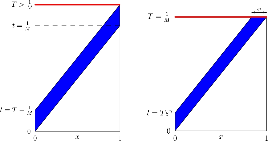
From (87), the first term vanishes because for all . Moreover, for , the segment for belongs to . Consequently, the second term vanishes as well and , for all . In particular , for all . Then, the relation (40) implies that the function satisfies for all , for all . Consequently, the function defined by (44) satisfies on . The result follows from the inequality and Theorem 2.2. Figure 2-left illustrates this result. □
Influence zone of the control (as ) in delimited by the characteristic line for and .
From a controllability viewpoint, the null function is a much better approximate null control than the function we construct in Proposition 3.2. The interest of such proposition (and of the results presented in the previous section) lies on the asymptotic of the solution of a direct problem. Given any function , we may approximate numerically the corresponding solution and get an approximation, says , where h is a discretization parameter. The error will be of the order , for some rate (see [3]). For ε small enough and m large enough, this error will be larger than . We emphasize that the function is easily calculable because explicit for all .
The limit case can be considered as well but requires explicit formula. The function is no longer equal to zero in this case. Let us consider for simplicity the case for which
so that
First, (16) leads to . Therefore,
Writing that and that , we obtain that
Moreover, from (11), we obtain, for all , that
and we may easily define a function such that the norm be equal to zero. Actually, since the function is supported in , it suffices to take a function such that for , i.e. supported in (see Fig. 2-right). Consequently, such control leads to
It remains to evaluate the term , equivalently evaluate the term . In order to satisfy the matching conditions of Lemma 2.1, we define as follows
for any -function such that with . The function (and in particular the derivatives) depends on ε here and so the constant in (53).
Let us evaluate the first term of (see (54)), restricted to , in function of the support of : from , we have
Let us consider the polynomial of order 3 given by so that and for all . Moreover, to simplify even more the computation, let assume that so that the control is simply given by leading to and then (from (89))
We are therefore looking for such that as . We take . This requires and then .
We can proceed in a similar way with the other terms in (54) and determine a rate such that and then . This allows to conclude that there exists a control function such that the solution of (8) with satisfies
with (instead of in Proposition 3.2). This stronger condition shows how the convergence is affected in the limit case . Nevertheless, after tedious computations, we may extend this construction of to any order k and improve the rate in the estimate (90). This may allow to obtain a better estimate that in the uncontrolled case discussed in Proposition 3.1. Remark that in the uncontrolled case, the norm is a priori not exponentially small for .
The case of initial condition dependent on ε
The asymptotic analysis performed in Section 2 requires a priori more care if the initial condition depends on the parameter ε. Due to the compatibility conditions of Lemma 2.6, the control functions may then depend on ε (at least in the neighborhood of ) and so the constant in (65).
In view of the initial condition defined in (4) (highlighted in [2,13]), we have in particular in mind the initial data of the form , with , . Such initial data get concentrated as at the point (resp. ) for (resp. ). Precisely, let us consider the case of the initial data (4):
such that . Taking in Lemma 2.7, the function involves the term where is given by (11). In particular, for points below the characteristic, that is in the set , we obtain ; this leads, after some computations, to (writing that on )
Consequently, cannot be a convergent approximation of , as , and a higher approximation is required! In view of the linearity of (1), we can expect for (assuming that ) an approximation, say , such that and therefore an approximation of such that
Taking large enough, we can therefore determine a convergent approximation of provided compatibility conditions between and the control , . The estimation of may however require tedious computations.
A possible alternative to address initial condition like (91) is to preliminary perform a change of unknown taking into account the exponential function. The one used in the proof of Lemma 2.3 is prohibited as it makes appear a term with coefficient (see 36). Still in view of (91), let us assume that the initial condition is of the form where f is an arbitrary function independent of ε, and . We introduce the following change of unknown
We then check that
with . Consequently, the new unknown solves
The initial data is now independent of ε. On the contrary, the control depends a priori on ε. We have thus reported the problem on the control part (which is relevant from a controllability viewpoint).
The asymptotic analysis for has been done in Section 2: it suffices to replace by . We define the asymptotic approximation of by
where the functions are defined as in Section 2. The corresponding control functions are noted by , . Finally, in view of (93), we define the approximation
so that . We are then looking for an approximation of the form
The main issue is now to find a set for the control functions satisfying the matching conditions of Lemma 2.6 such that goes to zero with ε. Again, the difficulty is that the control function , through the change of variable (93), may depend on ε. Adapting (54), we write that
with
To go on, let us consider again the simplest case for which . From (11),
we get
In view of the identity
and that , the function is negative on the set . We write
and compute that so that
We remark here the benefit of the change of unknown (93): with , the norm above goes to zero with ε (in contrast with (92)). Let now . We write (using (99)) that
The change of variable leads to
leading to for some and finally to
Let us now consider the second term in the expansion (97). Adapting (16), we have . Therefore
We check that for all so that the first term is negligible. For the second term, we make the change of variable ; we then check that
and then write
since for all . Moreover, the bound is strictly negative (for ε small enough), so that this term is once again negligible. With similar arguments, we conclude that the terms , and are exponentially small with respect to ε.
Therefore, we have the following result.
Let,, let,and. Let us consider the problemand assume thatandsatisfy the compatibility conditionsLet thenbe defined as follows:whereis given by (
98
) associated to the initial conditionand controland where.
Thenand there exists two constantsindependent of ε such that
Conditions (102) imply the property and . Therefore, in view of Lemma 2.6 for , and and then belongs to . Moreover, the function satisfies the following boundary value problem:
and therefore . The -norm of is exponentially small, since . Estimate (103) then follows from (100). □
For the initial condition (91) for which , , , (103) writes
where is a -function such that , . It suffices then that goes to zero with ε to ensure the approximation.
Actually, estimate (103) is mainly interesting from a controllability viewpoint as we may choose such that non only but also goes to zero with ε. For instance, if vanishes then and is an approximate control at time T for solution of (101) with initial data . In view of (96), if and only if . The function given by (98) is a solution of a transport equation and vanishes at time T if and only if the support of the control function is in . We do not detail here such construction for .
Conclusion
We have performed an asymptotic analysis of a singular advection-diffusion equation on the interval , with vanishing diffusion coefficient , positive transport coefficient, and Dirichlet control on . We have used the method of matched asymptotic expansions to construct an accurate asymptotic approximation of the solution of the direct problem. The construction is performed at any order m. Assuming that is in the form , the functions and the initial data are smooth and satisfy some compatibility conditions, we have constructed the inner and outer solutions by using explicit formulae. The asymptotic approximation is obtained by combining the inner and outer solutions through a process of matching. Note that the asymptotic approximation is very useful, for instance, from a numerical viewpoint (easily computable because using explicit formulae).
We have proved that is a regular and strong convergent approximation of , as , and established an error estimate (see Theorem 2.2). For the adjoint solution we have performed a similar asymptotic analysis.
We also provided sufficient conditions on the control functions and on allowing to pass to the limit, as , with ε small enough but fixed (see Theorem 2.3).
As a consequence of our asymptotic analysis, we constructed explicitly approximate controls leading to polynomially small (with respect to ε) state at any time .
The knowledge of the minimal uniform controllability time remains unknown for an arbitrary initial condition. One may use our asymptotic analysis in the optimality system (6) which characterizes the unique control of minimal -norm, and the initial condition (assumed independent of ε) being fixed. Let us focus on the optimality equation which links the forward and backward solutions. Using the inner expansion for (see Section 2.5), this equality rewrites as follows
At the zero order, we get therefore the equality leading, using (81) and (83) simultaneously, to
The function defined in is given by (81). It , the last equality contradicts the matching conditions (45), notably , unless ! If , we have , and in particular . But again, this contradicts (86) unless (and so ). In order to avoid this difficulty, we must relax the matching conditions (46) and (86) and therefore take into account the second boundary layer occurring for and on the characteristic lines and , respectively. This will be done in a forthcoming work. The negative case , which is similar, will be addressed as well.
References
1.
H.Brezis, Functional Analysis, Sobolev Spaces and Partial Differential Equations, Universitext, Springer, New York, 2011.
2.
J.-M.Coron and S.Guerrero, Singular optimal control: A linear 1-D parabolic-hyperbolic example, Asymptot. Anal.44 (2005), 237–257.
3.
P.Deuring, R.Eymard and M.Mildner, -stability independent of diffusion for a finite element-finite volume discretization of a linear convection-diffusion equation, SIAM J. Numer. Anal.53 (2015), 508–526. doi:10.1137/140961146.
4.
A.V.Fursikov and O.Y.Imanuvilov, Controllability of Evolution Equations, Lecture Notes Series, Seoul National University Research Institute of Mathematics, Vol. 34, Global Analysis Research Center, Seoul, 1996.
5.
O.Glass, A complex-analytic approach to the problem of uniform controllability of a transport equation in the vanishing viscosity limit, Journal of Functional Analysis258 (2010), 852–868. doi:10.1016/j.jfa.2009.06.035.
6.
S.Guerrero and G.Lebeau, Singular optimal control for a transport-diffusion equation, Comm. Partial Differential Equations32 (2007), 1813–1836. doi:10.1080/03605300701743756.
7.
J.Kevorkian and J.D.Cole, Multiple Scale and Singular Perturbation Methods, Applied Mathematical Sciences, Vol. 114, Springer-Verlag, New York, 1996.
8.
S.G.Krantz and H.R.Parks, A Primer of Real Analytic Functions, 2nd edn, Birkhäuser Advanced Texts: Basler Lehrbücher. [Birkhäuser Advanced Texts: Basel Textbooks], Birkhäuser Boston, Inc., Boston, MA, 2002.
9.
G.Lebeau and L.Robbiano, Contrôle exact de l’équation de la chaleur, Comm. Partial Differential Equations20 (1995), 335–356. doi:10.1080/03605309508821097.
10.
J.-L.Lions, Perturbations Singulières dans les Problèmes aux Limites et en Contrôle Optimal, Lecture Notes in Mathematics, Vol. 323, Springer-Verlag, Berlin-New York, 1973.
11.
J.-L.Lions, Contrôlabilité Exacte, Perturbations et Stabilisation de Systèmes Distribués. Tome 2, Recherches en Mathématiques Appliquées [Research in Applied Mathematics], Vol. 9, Masson, Paris, 1988, Perturbations. [Perturbations].
12.
P.Lissy, A link between the cost of fast controls for the 1-d heat equation and the uniform controllability of a 1-d transport-diffusion equation, Comptes Rendus Mathematique350 (2012), 591–595. doi:10.1016/j.crma.2012.06.004.
13.
P.Lissy, Explicit lower bounds for the cost of fast controls for some 1-D parabolic or dispersive equations, and a new lower bound concerning the uniform controllability of the 1-D transport-diffusion equation, J. Differential Equations259 (2015), 5331–5352. doi:10.1016/j.jde.2015.06.031.
14.
F.Marbach, Small time global null controllability for a viscous Burgers’ equation despite the presence of a boundary layer, J. Math. Pures Appl.9(102) (2014), 364–384. doi:10.1016/j.matpur.2013.11.013.
15.
A.Münch, Numerical estimation of the cost of boundary controls for the equation with respect to ε, SEMA-SIMAI Springer series – Recent Advances in PDEs: Analysis, Numerics and controls, 2018, in honor of Prof. Enrique Fernandez-Cara’s 60 birthday, 17.
16.
Y.Ou and P.Zhu, The vanishing viscosity method for the sensitivity analysis of an optimal control problem of conservation laws in the presence of shocks, Nonlinear Anal. Real World Appl.14 (2013), 1947–1974. doi:10.1016/j.nonrwa.2013.02.001.
17.
J.Sanchez Hubert and E.Sánchez-Palencia, Vibration and Coupling of Continuous Systems, Springer-Verlag, Berlin, 1989, Asymptotic methods.
18.
M.Van Dyke, Perturbation Methods in Fluid Mechanics, annotated edn, The Parabolic Press, Stanford, Calif., 1975.