Asymptotical analysis of a nonlinear Sturm–Liouville problem: Linearisable and non-linearisable solutions

Abstract

The paper focuses on a nonlinear eigenvalue problem of Sturm–Liouville type with real spectral parameter under first type boundary conditions and additional local condition. The nonlinear term is an arbitrary monotonically increasing function. It is shown that for small nonlinearity the negative eigenvalues can be considered as perturbations of solutions to the corresponding linear eigenvalue problem, whereas big positive eigenvalues cannot be considered in this way. Solvability results are found, asymptotics of negative as well as positive eigenvalues are derived, distribution of zeros of the eigenfunctions is presented. As a by-product, a comparison theorem between eigenvalues of two problems with different data is derived. Applications of the found results in electromagnetic theory are given.

Keywords

Nonlinear Sturm–Liouville problem asymptotical analysis distribution of eigenvalues comparison theorem periodicity of eigenfunctions

1. Introduction

By now theory of nonlinear Sturm–Liouville problems is extremely voluminous and, in fact, it is not easy (if at all possible) to give a comprehensive review of this field [5,9,16,17,25,34]. Moreover, the description of the field depends essentially on the researcher’s point of view. Nevertheless, if one is interested in problems having isolated eigenvalues, then the whole theory can be divided into two big areas: (a) Sturm–Liouville problems that depend linearly on the sought-for function and nonlinearly on the spectral parameter; (b) Sturm–Liouville problems that depend nonlinearly on the sought-for function and linearly/nonlinearly on the spectral parameter.

Problems from the former area can be studied with powerful methods such as variational techniques, operator pencil and operator-function approaches [12,15,21].

We, however, pay attention to the latter area, that is, we are interested in problems that are nonlinear in the sought-for function. In this case, we speak about a (nonlinear) Sturm–Liouville problem for a quasilinear autonomous/non-autonomous differential equation of the second order on a finite segment. The main question, obviously, is to prove existence of eigenvalues and determine its properties. As is well-known in order to get isolated eigenvalues, in addition to (two) boundary conditions (of the first, second, or third type, or even more complicated) on both sides of the segment, one has to impose one more condition, see, for example, [14]. There are two opportunities: nonlocal or local condition.

One of the most frequently used nonlocal conditions is a condition of the form $‖ u ‖_{G}^{2} = const$ in an appropriate function space G, where u is a sought-for function and $const$ is given (u, in fact, is an eigenfunction). In this case there are powerful variational techniques to study such problems, see [4,5,16,17,24,25,30,34] and the bibliography therein.

Local additional condition in the simplest case can be written in the form $u |_{x = x_{0}} = const$ (or $u^{'} |_{x = x_{0}} = const$ ), where u is a sought-for (eigen)function, $x_{0}$ is a particular point belonging to the considered finite segment, and $const$ is given [14,16,31,37,39]. Clearly, an additional local condition does not allow using variational approaches.

In spite of the great advance in the nonlinear Sturm–Liouville theory achieved with the aforementioned methods and approaches, in this paper we would like to develop, as far as we know, a novel tool to study a particular class of nonlinear Sturm–Liouville problems with additional local condition. In order to introduce our approach we remind some well known ideas from the classical (linear) Sturm–Liouville theory. One of the good ways to study a linear Sturm–Liouville problem is to consider its characteristic function. Eigenvalues of the Sturm–Liouville problem are roots of the so called characteristic equation (or zeros of the characteristic function) and vice versa [20]. In this research, studying a nonlinear Sturm–Liouville problem, we develop an approach that leads to a transcendental equation with respect to the spectral parameter. Roots of this equation are eigenvalues of the nonlinear problem and vice versa. Thus the below derived equation can be treated as the characteristic equation of the Sturm–Liouville problem; due to its form, which is expressed as an integral relation, it is natural to call it integral characteristic equation (ICE). Using ICE, one can define the integral characteristic function (ICF). Applying asymptotical analysis to the behaviour of ICF, one can derive existence of its zeros and find asymptotics of the zeros. In other words, using an original technique, one can derive results about solvability of the nonlinear problem and properties of its solution. The developed approach does not rely on smallness of any parameters of the problem and allows one to prove existence of eigenvalues without linear counterparts.

At last we also add that a wide class of nonlinear Sturm–Liouville problems can be studied by perturbation methods, where the non-perturbed problems are linear ones, see, for example, [16,28]. A more complicated approach based on perturbation methods relates to the existence of so-called non-perturbative solutions of some nonlinear Sturm–Liouville problems [18,32]. Such an approach, however, is only applicable to multiparameter nonlinear Sturm–Liouville problems. We call a solution to be a non-perturbative (or non-linearisable) one if this solution has no linear counterpart.

Well, the paper is written in accordance with the following outline: statement of the problem is presented in Section 2; ICE is derived in Section 3; solvability of the problem $P$ is studied in Section 4; applications in the nonlinear optics are shown in Section 5; conclusions are given in Section 6; proofs are presented in Section 7 (we decided to detach the proofs from the statements and theorems in order that the readers can quickly penetrate the results without looking aside).

The most important and auxiliary results we formulate as theorems and statements, respectively. We also note that using the term solvability with respect to the problem $P$ we mean results about existence of eigenvalues of this problem; in other cases the meaning of the term solvability is clear.

2. Statement of the problem

Let $I = (0, h)$ , where $h > 0$ is a constant, and $\bar{I} = [0, h]$ ; in addition, constants $a, α, A \in R_{+}$ , where $R_{+} = (0, + \infty)$ , and λ is a real parameter.

The problem $P$ consists in finding real values of the (spectral) parameter λ for which there exist twice differentiable in x solutions $u \equiv u (x; λ)$ to equation $\begin{matrix} (1) & u^{″} = - (a - λ + α f (u^{2})) u, x \in \bar{I} \end{matrix}$ that satisfy boundary and initial data $\begin{matrix} (2) & u (0; λ) = 0, u^{'} (0; λ) = A, u (h; λ) = 0, \end{matrix}$ where $f \in C^{1} [0, + \infty)$ is a monotonically increasing function and $f (0) = 0$ .

Definition 1.
A value $λ = \hat{λ} \in R$ such that for prescribed value $u_{x = 0}^{'} \neq 0$ (without loss of generality $u_{x = 0}^{'} > 0$ ) there exists a twice differentiable function $u \equiv u (x; \hat{λ})$ that satisfies (1)–(2), is called an eigenvalue of the problem $P$ , and the function $u (x; \hat{λ})$ , corresponding to the eigenvalue $\hat{λ}$ , is called an eigenfunction of the problem $P$ .

Negative and positive eigenvalues of the problem $P$ are denoted by ${\hat{λ}}^{-}$ and ${\hat{λ}}^{+}$ , respectively, or by ${\hat{λ}}_{n}^{\pm}$ , where n is a nonnegative integer; in the latter case one supposes that ${\hat{λ}}_{n}^{-}$ and ${\hat{λ}}_{n}^{+}$ are arranged in the descending and ascending orders, respectively.
Remark 1.
Definition 1 is a nonclassical analog of the well-known definition of a characteristic value of a linear operator-function nonlinearly depending on the spectral parameter [12].

We stress that widely known methods of nonlinear analysis like variational methods [4,17,25,34], bifurcation and ramification theories [16,17,34] as well as perturbation methods based on linear problems [15] are not applicable to derive solvability results in the problem $P$ especially for big positive λ.

Let us consider the linear problem (for $α = 0$ ), which is called problem $P_{0}$ . Negative and positive eigenvalues of the problem $P_{0}$ are denoted by ${\tilde{λ}}^{-}$ and ${\tilde{λ}}^{+}$ , respectively, or by ${\tilde{λ}}_{n}^{\pm}$ , where n is a nonnegative integer; in the latter case one supposes that ${\tilde{λ}}_{n}^{-}$ and ${\tilde{λ}}_{n}^{+}$ are arranged in the descending and ascending orders, respectively. If it does not lead to misunderstanding, for the eigenvalues of the problems $P$ and $P_{0}$ we also use the notation $\hat{λ}$ , ${\hat{λ}}_{n}$ and ${\tilde{λ}}_{n}$ , respectively.

It is well-known (and can easily be checked) that the following result is true.
Statement 1.
The problem $P_{0}$ has infinitely many simple negative and a finite number (or does not have at all) of simple positive eigenvalues; the asymptotical behaviour of the negative eigenvalues is characterised by the formula ${\tilde{λ}}_{n - 1} = O (n^{2})$ .

The eigenvalues $λ = {\tilde{λ}}^{\pm}$ of problem $P_{0}$ are (simple) roots of the characteristic equation $\begin{matrix} (3) & sin \sqrt{a - λ} h = 0 . \end{matrix}$ Solving equation (3), one finds exact expression for the eigenvalues of the problem $P_{0}$ . To be more precise, one has $\begin{matrix} (4) & {\tilde{λ}}_{n}^{+} = a - \frac{π^{2} n^{2}}{h^{2}} with 0 < n < n_{0} and {\tilde{λ}}_{n}^{-} = a - \frac{π^{2} n^{2}}{h^{2}} with n ⩾ n_{0}, \end{matrix}$ where $n_{0}$ is a positive integer such that $a h^{2} - π^{2} n_{0}^{2} > 0$ and $a h^{2} - π^{2} {(n_{0} + 1)}^{2} < 0$ .
3. Integral characteristic equation

Let us consider the Cauchy problem for equation (1) with initial data $\begin{matrix} (5) & u (0; λ) = 0, u^{'} (0; λ) = A . \end{matrix}$ We are going to derive the global unique solvability of the Cauchy problem (1), (5), which then be used to study solvability of the problem $P$ .

Multiplying (1) by $u^{'}$ , integrating and using (5), one obtains $\begin{matrix} (6) & u^{' 2} + (a - λ) u^{2} + α F (u^{2}) \equiv A^{2}, \end{matrix}$ where $F (u^{2}) = \int_{0}^{u^{2}} f (t) d t$ .

Substituting $x = h$ into (6), using (2), one finds the equation $B^{2} = A^{2}$ , where $B : = u^{'} (h)$ . This equation has only two real solutions $B = \pm A$ .

Introduce new variables $\begin{matrix} (7) & τ (x) = u^{2} (x), η (x) = \frac{u^{'} (x)}{u (x)} . \end{matrix}$

Using conditions (5), one finds $\begin{matrix} (8) & lim_{x \to + 0} η (x; λ) = + \infty . \end{matrix}$

Using transformation (7) and equation (1), the equation (6) can be rewritten as $\begin{matrix} (9) & \{\begin{matrix} τ^{'} = 2 τ η, \\ η^{'} = - (a - λ + α f (τ) + η^{2}) . \end{matrix} \end{matrix}$ The first integral of system (9) can be found straightforwardly from (9) or by direct substitution of $u^{2}$ and $u^{' 2}$ in (6) with variables (7); it has the form $\begin{matrix} (10) & (η^{2} + a - λ) τ + α F (τ) \equiv A^{2} . \end{matrix}$

Since equation (10) implicitly defines function $τ \equiv τ (η; λ)$ , then the second equation of system (9) can be rewritten as $η^{'} = - w (η; λ)$ , where $\begin{matrix} (11) & w (η; λ) \equiv η^{2} + a - λ + α f (τ (η; λ)) . \end{matrix}$

It is easy to check that $w (η; λ) > 0$ for all λ. Indeed, assuming that w vanishes at some point and equating w to zero, one obtains $η^{2} + a - λ = - α f (τ)$ . Using the found relation together with (10), one gets $A^{2} = α F (τ) - α f (τ) τ = - α \int_{0}^{τ} f^{'} (s) s d s$ . Since f monotonically increases, then $f^{'} > 0$ ; therefore the left- and right-hand sides of expression $A^{2} = - α \int_{0}^{τ} f^{'} (s) s d s$ are of different signs. This contradiction proves that $w (η; λ) > 0$ for all $λ \in R$ .

It follows from the second formula (7) that $η (x; λ)$ is continuous for $x \in I$ if and only if $u (x; λ)$ does not vanish for $x \in I$ . Suppose that u has $n ⩾ 0$ zeros $x_{1}, \dots, x_{n} \in I$ . Then η has n break points $x_{1}, \dots, x_{n}$ . It is clear that if $u ≢ 0$ then $u^{'} (x_{i}) \neq 0$ for all $i = \overline{1, n}$ . Indeed, if a solution u to equation (1) and its derivative $u^{'}$ vanish at the same point, then $u \equiv 0$ due to classical results on the (local) existence and uniqueness of the Cauchy problem [13]. Thus the break points are break points of the second kind.

Taking into account that $η^{'} = - w (η; λ) < 0$ , one comes to the conclusion that $η (x; λ)$ monotonically decreases and, therefore, using (7), one derives that $\begin{matrix} (12) & η (x_{i} - 0) = - \infty, η (x_{i} + 0) = + \infty, where i = \overline{1, n} . \end{matrix}$

Integrating equation $η^{'} = - w (η; λ)$ on every interval $(0, x_{1}), (x_{1}, x_{2}), \dots, (x_{n}, h)$ and using conditions (12), one gets

Statement 2.
The Cauchy problem ( 1 ), ( 5 ) is globally unique solvable and its (classical) solution $u \equiv u (x; λ)$ continuously depends on $(x, λ, α) \in \bar{I} \times R \times R_{+}$ . In addition, formula $\begin{matrix} (13) & n \int_{- \infty}^{+ \infty} \frac{d s}{w (s; λ)} + \int_{η (h; λ)}^{+ \infty} \frac{d s}{w (s; λ)} = h \end{matrix}$ is valid, where $n ⩾ 0$ is the number of zeros of the solution $u \equiv u (x; λ)$ for $x \in I$ and, in general, $η (h; λ)$ is not prescribed.

In connection with Statement 2, see also [31].

Taking into account (2) and using monotonicity of the function $η (x; λ)$ , one gets $\begin{matrix} (14) & η (h; λ) = - \infty . \end{matrix}$

Well, it follows from formulas (8), (12), and (14) that if u is an eigenfunction of the problem $P$ , then the function η takes all real values. It turns out that if $η \in R$ , then in some cases λ cannot take all values from $R$ . It is known from above that if $w (s; λ)$ exists, then it is always positive. However the function $τ \equiv τ (η; λ)$ may not exist for some λ and, therefore, for such λ the function $w (s; λ)$ does not exist as well. The least value λ for which the (positive) function τ does not exist we denote by $λ_{max}$ . It is easily seen from (10) that $λ_{max} > 0$ . If $τ > 0$ exists for any $λ \in R$ , then $λ_{max} = + \infty$ .

The following statement gives exact values for $λ_{max}$ .
Statement 3.
Let the solution $u \equiv u (x; λ)$ to the Cauchy problem ( 1 ), ( 5 ) have at least one zero on $(0, h]$ . If f is an unbounded function, then $λ_{max} = + \infty$ ; if f is a bounded function, then $λ_{max} = a + α f_{max}$ , where $f_{max} = {lim}_{s \to + \infty} f (s)$ .

Below we always assume that $λ \in Λ$ , where $Λ : = (- \infty, λ_{max})$ .

Relation (13) under condition (14) results in ICE of the problem $P$ , that is, one has $\begin{matrix} (15) & Φ (λ; n) \equiv (n + 1) T (λ) = h, \end{matrix}$ where $n = 0, 1, \dots$ , $T (λ) = \int_{- \infty}^{+ \infty} \frac{d s}{w (s; λ)}$ .

ICE (15) is a family (but not a system) of equations for different n. The function $Φ (λ; n) - h$ is called integral characteristic function (ICF).

The equivalence between the problem $P$ and ICE (15) is established in the following theorem.
Theorem 1 (of equivalence).

The value $\hat{λ} \in Λ$ is a solution to the problem $P$ if and only if there exists an integer $\hat{n} ⩾ 0$ such that $λ = \hat{λ}$ satisfies ( 15 ); the corresponding eigenfunction $u \equiv u (x; \hat{λ})$ has $\hat{n}$ (simple) zeros $x_{i} = i T (\hat{λ})$ , where $i = \overline{1, \hat{n}}$ and $x_{i} \in I$ .

We stress that Statement 2 does not contradict Theorem 1. Indeed, the Cauchy problem (1), (5) involves only initial data (5). At the same time, ICE (15) involves conditions at both endpoints (2). In other words, the searched-for solution to the Cauchy problem does not necessarily vanish for $x \in (0, h]$ , whereas any of the eigenfunctions does, see also the last paragraph in the proof of Statement 3.

Remark 2.
It follows from Theorem 1 that if $λ = \hat{λ}$ is a solution to ICE (15), then the eigenfunction $u (x; \hat{λ})$ has $\hat{n}$ zeros. In the problem $P$ there can exist eigenfunctions corresponding to different eigenvalues, but having the same number of zeros. In the problem $P_{0}$ , there exists at most one eigenfunction with a given number of zeros.

Theorem 1 gives a reason for the following definition.
Definition 2.
If $λ = \hat{λ}$ is root of a multiplicity p to ICE (15), then $\hat{λ}$ is an eigenvalue of the problem $P$ of the same multiplicity.

The following result is valid.
Statement 4.
The function $T (λ)$ defined by ( 15 ) is continuous and positive for all $λ \in Λ$ .

Since proving periodicity property and finding exact formula for the period are important questions in the theory of nonlinear (autonomous) equations [6,23,27], then the following result can be of interest. Theorem 2 (of periodicity).

Let $λ = \hat{λ}$ be an eigenvalue of the problem $P$ and $u \equiv u (x; \hat{λ})$ be the corresponding eigenfunction. If u has more than one zero inside I, then u is a periodic function with the period $Θ = 2 T (\hat{λ})$ .

4. Existence of eigenvalues

Let $\begin{matrix} h_{inf}^{(k)} : = inf_{λ \in Λ} Φ (λ; k), h_{sup}^{(k)} : = sup_{λ \in Λ} Φ (λ; k), k = 0, 1, \dots \end{matrix}$

It follows from Statement 4 that $h_{inf}^{(k)}$ always exists and has a (finite) positive value. If there exists $λ \in Λ$ such that $Φ (λ; k)$ tends to infinity, then we set $h_{sup}^{(k)} = + \infty$ . It is clear that $Φ (λ; k)$ can tend to infinity only if $λ \to λ_{max}$ .

Sufficient conditions for existence of at least one eigenvalue is given by the following theorem.

Theorem 3.
Suppose $h_{inf}^{(k)} < h_{sup}^{(k)}$ for some $k = k^{'}$ and h such that $h_{inf}^{(k^{'})} < h < h_{sup}^{(k^{'})}$ ; then the problem $P$ has at least one solution $\hat{λ}$ .

Let $Δ = [0, + \infty) \subset R$ , and $B_{δ} (x)$ be an open ball of radius δ centred at the point x, where $δ > 0$ is a fixed value. Denote by $R_{Δ}^{δ} = ⋃_{x \in Δ} B_{δ} (x)$ an (open) neighbourhood of the set Δ on the complex plane $C$ . Then the following result takes place.
Statement 5.
The function $τ (η; γ)$ , implicitly defined by ( 10 ), exists, is continuous and positive for all $(η, λ) \in R \times Λ$ . In addition, if $f \equiv f (z)$ is an analytic function for $z \in R_{Δ}^{δ} \subset C$ , then the function $τ (η; λ)$ analytically depends on λ for $λ \in Λ$ .

The following fact results from Statement 5.
Theorem 4.
Suppose $h_{inf}^{(k)} < h_{sup}^{(k)}$ for all nonnegative integer k, $f (z)$ is an analytic function for $z \in R_{Δ}^{δ} \subset C$ , and h is such that $h_{inf}^{(k^{'})} < h < h_{sup}^{(k^{'})}$ for some $k = k^{'}$ ; then the set of eigenvalues of the problem $P$ is not empty and is discrete on Λ, that is, each segment $Λ^{'} \subset Λ$ contains no more than a finite number of (isolated) eigenvalues.

Let us suppose that the (linear) problem $P_{0}$ has k eigenvalues ${\tilde{λ}}_{i}$ ; then if the constant $α (> 0)$ is sufficiently small, one can prove existence of eigenvalues of the problem $P$ that are close to solutions ${\tilde{λ}}_{i}$ of the problem $P_{0}$ .

We begin with the following statement.
Statement 6.
If $λ < a$ , then ${lim}_{α \to + 0} Φ (λ; n) = Φ_{0} (λ; n)$ , where $n ⩾ 0$ is an integer, and equation $\begin{matrix} (16) & Φ_{0} (λ; n) \equiv (n + 1) T_{0} (λ) = h, \end{matrix}$ where $T_{0} (λ) = \int_{- \infty}^{+ \infty} \frac{d s}{s^{2} + a - λ}$ , is valid.

Using Statement 6, one obtains the following perturbation theorem.
Theorem 5.
Let ${\tilde{λ}}_{i}$ , where $i = \overline{k_{1}, k_{2}}$ , $| k_{1} - k_{2} | = k$ , and k is finite, be k eigenvalues of the problem $P_{0}$ . There exists a constant $α^{″} > 0$ such that for any positive $α = α^{'} < α^{″}$ there exist at least k eigenvalues ${\hat{λ}}_{i}$ of the problem $P$ , where ${\hat{λ}}_{i} < a$ and ${lim}_{α^{'} \to + 0} {\hat{λ}}_{i} = {\tilde{λ}}_{i}$ .

Below we use the following result.
Statement 7.
The function $T (λ)$ can be written in the form $\begin{matrix} (17) & T (λ) \equiv \int_{0}^{τ_{+}} \frac{d τ}{v (τ; λ)}, \end{matrix}$ where $v (τ; γ) = \sqrt{τ} \sqrt{A^{2} - (a - λ) τ - α F (τ)}$ and $τ = τ_{+}$ is a (unique) positive root to the equation $\begin{matrix} (18) & A^{2} - (a - λ) τ - α F (τ) = 0 . \end{matrix}$

It is not necessary to impose additional conditions on f in order to determine the behaviour of the integrals in (15) for negative λ. Indeed, rewriting (10) in the form $(η^{2} + a - λ) = A^{2} - α F (τ)$ , one can easily see that if $λ ⩽ a$ , then the written relation defines a unique positive function $τ \equiv τ (η; λ)$ that is estimated as $0 < τ < τ_{-} < A^{2} / α$ , where $τ = τ_{-}$ is a unique positive solution to equation $A^{2} - α F (τ) = 0$ . Using these inequalities, one comes to the following estimations.
Statement 8.
If $λ < δ < a$ , where $δ > 0$ is a constant, then the estimations $\begin{matrix} (19) & \frac{π}{\sqrt{a - λ + α f_{-}}} < T (λ) < \frac{π}{\sqrt{a - λ}} \end{matrix}$ are valid, where $f_{-} = f (τ_{-}) < f (A^{2} / α)$ .

Behaviour of $T (λ)$ crucially depends on f only as $λ \to λ_{max}$ . This is the reason why we separately study three different cases: power, logarithmic, and bounded growth of f for big τ.

Using Statement 8, one can easily derive solvability of the problem $P$ for $λ < a - δ$ , where $δ > 0$ is a constant. To be more precise, the following result is valid.
Theorem 6.
The problem $P$ has infinitely many negative eigenvalues ${\hat{λ}}_{n}^{-}$ with the asymptotics $\begin{matrix} (20) & {\hat{λ}}_{n - 1}^{-} = O^{} (n^{2}) . \end{matrix}$ In addition, for all sufficiently big indexes n the following comparison result* $\begin{matrix} (21) & {\tilde{λ}}_{n}^{-} < {\hat{λ}}_{n}^{-} < {\tilde{λ}}_{n + 1}^{-}, \end{matrix}$ where ${\tilde{λ}}_{n}^{-}$ is the nth negative eigenvalue of the problem $P_{0}$ , takes place.

Further results on the eigenvalues of the problem $P$ are obtained with additional conditions on f and without assumption on the smallness of α.
4.1. Power growth of f

Let $f \in C^{1} [0, + \infty)$ be a monotonically increasing function, $f (0) = 0$ , and be characterised by the following behaviour $\begin{matrix} (22) & f (u^{2}) = | u |^{2 q} + f_{1} (u^{2}) as u = \pm \infty, \end{matrix}$ where ${lim}_{u \to \pm \infty} \frac{f_{1} (u^{2})}{| u |^{2 q}} = 0$ and $q > 0$ . Thus $\begin{matrix} (23) & F (τ) = \frac{τ^{q + 1}}{q + 1} + F_{1} (τ) as τ \to + \infty, \end{matrix}$ where $F_{1} (τ) = \int_{0}^{τ} f_{1} (s) d s$ and ${lim}_{τ \to + \infty} \frac{F_{1} (τ)}{τ^{q + 1}} = 0$ .

Under above listed conditions, the behaviour of $T (λ)$ is given by the following statement.

Statement 9.
For sufficiently big positive λ it is true that $\begin{matrix} (24) & T (λ) = (1 + q^{- 1}) λ^{- 1 / 2} ln λ + O (λ^{- 1 / 2}) . \end{matrix}$

The following theorem claims solvability of the problem $P$ for positive λ.
Theorem 7.
The problem $P$ has infinitely many (positive) eigenvalues ${\hat{λ}}_{i}^{+} \in Λ$ with an accumulation point at infinity. Furthermore,
for big $\hat{λ}$ the following asymptotics $\begin{matrix} (25) & {\hat{λ}}_{m - 1}^{+} = O^{} (f_{m}) \end{matrix}$ is valid, where* $f_{m} = g^{- 1} (\frac{h q}{m (q + 1)})$ , $λ = {\hat{λ}}_{m}^{+}$ is a solution to ICE ( 15 ) for $n = m$ , and $g^{- 1}$ is the inversion of $g (t) = t^{- 1 / 2} ln t$ ;

${max}_{x \in [0, h]} | u (x; t) | = O (t^{\frac{1}{2 q}})$ , where $t = {\hat{λ}}_{n}^{+}$ , for all sufficiently big n.

Remark 3.
If i is sufficiently large, then there is no connection between the eigenvalues ${\hat{λ}}_{i}^{+}$ and solutions to the (linear) problem $P_{0}$ as $α \to + 0$ .

Comparison theorems are known to be classical in the (linear) Sturm–Liouville theory [33]. Below we present such a result for the nonlinear case; this result is a by-product theorem obtained using the developed method.

Now we denote $P$ by $P (q)$ , where q characterizes the growth of the function f, and consider two problems $P (q_{1})$ and $P (q_{2})$ . Theorem 7 states that each of these problems has an infinite number of eigenvalues $λ = {\hat{λ}}_{1, i}^{+}$ and $λ = {\hat{λ}}_{2, i}^{+}$ , respectively, where ${lim}_{i \to \infty} {\hat{λ}}_{j, i}^{+} = + \infty$ ( $j = 1, 2$ ). Well, the following result takes place. Theorem 8.
If $q_{1} < q_{2}$ , then the inequality ${\hat{λ}}_{1, i}^{+} > {\hat{λ}}_{2, i}^{+}$ is valid for all sufficiently big indexes i.

4.2. Logarithmic growth of f

Let $f (u^{2}) = ln (1 + u^{2})$ . In this case the behaviour of $T (λ)$ is given by the following statement.

Statement 10.
For sufficiently big positive λ it is true that $\begin{matrix} (26) & T (λ) ⩾ \frac{\sqrt{λ}}{2 α} + \frac{ln λ}{\sqrt{λ}} + O (λ^{- 1 / 2}) . \end{matrix}$

Using Statements 5 and 10, one obtains the following corollary. Corollary 1.
There exists a constant $h_{min} > 0$ such that for any $h > h_{min}$ the problem $P$ has a finite number (and at least one) of (positive) isolated eigenvalues ${\hat{λ}}_{i}^{+}$ . For any ${\hat{λ}}_{i} \in (0, a)$ it is true that ${lim}_{α \to + 0} {\hat{λ}}_{i}^{+} = {\tilde{γ}}_{i}^{+}$ , where ${\tilde{λ}}_{i}^{+}$ is a solution to the problem $P_{0}$ .

4.3. Bounded growth of f

Let function $f (z)$ be analytic with respect to z for $z \in R_{Δ}^{δ}$ , be monotonically increasing and bounded above, and $f (0) = 0$ . In this case the behaviour of $T (λ)$ is given by the following statement.

Statement 11.
For positive λ it is true that $\begin{matrix} \frac{π}{\sqrt{a + α f_{max} - λ}} < T (λ) < \frac{π}{\sqrt{a - λ}} \end{matrix}$ and ${lim}_{λ \to λ_{max}} T (λ) = + \infty$ , where $λ_{max} = a + α f_{max}$ , and $f_{max} = {lim}_{s \to + \infty} f (s)$ .

Using Statements 5 and 11, one obtains the following corollary. Corollary 2.
There exists a constant $h_{min} > 0$ such that for any $h > h_{min}$ the problem $P$ has a finite number (and at least one) of positive isolated eigenvalues ${\hat{λ}}_{i}^{+}$ . For any ${\hat{λ}}_{i} \in (0, a)$ it is true that ${lim}_{α \to + 0} {\hat{λ}}_{i}^{+} = {\tilde{γ}}_{i}^{+}$ , where ${\tilde{λ}}_{i}^{+}$ is a solution to the problem $P_{0}$ .

5. Physical background

For positive values of λ the problem $P$ describes propagation of transverse-electric (TE) guided waves in a plane dielectric waveguide filled with nonlinear medium and having perfectly conducting walls at $x = 0$ and $x = h$ . For a concerned reader, we briefly formulate the physical problem below.

Let $Σ = {(x, y, z) \in R^{3} : 0 ⩽ x ⩽ h, (y, z) \in R^{2}}$ be a layer located in $R^{3}$ ; it has perfectly conducted walls at the boundaries $x = 0$ and $x = h$ . We consider propagation of a monochromatic TE wave $(E, H) e^{- i ω t}$ in the layer Σ, where $\begin{matrix} (27) & E = {(0, e_{y}, 0)}^{⊤} \cdot e^{i γ z}, H = {(h_{x}, 0, h_{z})}^{⊤} \cdot e^{i γ z} \end{matrix}$ with $e_{y} \equiv e_{y} (x; γ)$ , $h_{x} \equiv h_{x} (x; γ)$ , $h_{z} \equiv h_{z} (x; γ)$ , and ω is the circular frequency, γ is an unknown real parameter (propagation constant of a guided wave). Comprehensive description of the linear theory of TE waves guide by a plane layer is presented in [1]; some related to this study results in the nonlinear theory can be found in [36,37], for a wide review, see also [8].

The permittivity in the layer Σ has the form $ϵ = ϵ_{l} + a_{l} f (| E |^{2})$ , where $a_{l} > 0$ is a real parameter, $ϵ_{l} > 0$ is a real constant, $f \in C^{1} [0, + \infty)$ is a monotonically increasing function, and $f (0) = 0$ . In the layer $μ = μ_{0} > 0$ is the permeability of vacuum. The field (27) satisfies Maxwells equations $\begin{matrix} (28) & \{\begin{matrix} rot H = - i ω ϵ E, \\ rot E = i ω μ H; \end{matrix} \end{matrix}$ the tangential component of the electric field vanishes at the perfectly conducted walls; the quantity $e_{y}^{'} |_{x = 0} = A \neq 0$ is supposed to be fixed (without loss of generality $A > 0$ ) [2,8,29,36,37].

It is necessary to find real γ such that there exists nontrivial field (27) satisfying the above given requirements.

Substituting (27) into (28), using the notation $u : = e_{y}$ , $ε : = ω^{2} μ ϵ$ , $α : = ω^{2} μ a_{l}$ , $a : = ω^{2} μ ϵ_{l}$ , and $λ : = γ^{2}$ , one arrives at (1). Physical conditions for the field (27) at the boundaries $x = 0$ and $x = h$ result in conditions (2).

The function f in (1) describes many important nonlinearities, in particular, polynomial and power nonlinearity. The polynomial nonlinearity arises from expanding the polarization vector in powers of the field [2,19,29]. Truncating this expansion to a finite number of terms, one obtains a nonlinearity in the form of a polynomial ( $q = 1, 2, 3$ represent the simplest of possible situations). Of particular significance in physics is the case of $q > 3$ . The power nonlinearity arises in nonlinear optics [2,8,19,29] and Schrödinger equation theory [10].

In the case of bounded growth of f, for example, nonlinearities $f \equiv 1 - e^{- β | E |^{2}}$ , $f \equiv \frac{| E |^{2}}{1 + β | E |^{2}}$ ( $β > 0$ ) satisfy the above required properties. These nonlinearities are used in nonlinear optics of waveguiding structures [2,3,38].

6. Conclusion

Well, the paper is devoted to the study of a nonlinear eigenvalue problem of Sturm–Liouville type, where the main equation depends nonlinearly on the sought-for function. The main two points, which we would like to stress in this section, are the following:

The paper suggests an original approach to study a particular class of (nonlinear) Sturm–Liouville problems for nonlinear autonomous ordinary differential equations of the second order. This approach is based on the use of the so called ICF and ICE related to the studied problem. We failed to find any similar technique in the literature and as we understand it, our approach is a novel and rigorous tool that has nothing in common with well known approaches based on variational methods. Moreover, the approach based on ICE allows one to study nonlinear eigenvalue problems that are out of reach variational techniques as well as bifurcation and ramification theories;

For the nonlinear eigenvalue problems mentioned above, the ICE approach allows one to derive existence of eigenvalues and determine its asymptotical behaviour. In addition, periodicity of the eigenfunctions and distribution of its zeros can also be established. This approach (if applicable) does not depend on the smallness of some parameters that the studied problem involves, that is, it can be used to determine linearisable as well as non-linearisable eigenvalues.

It should be noted that the ICE approach works well even if the studied problem depends nonlinearly on the spectral parameter also, see, for example, [35].

It is also significant that the area of applicability of the suggested approach extends further: some nonlinear multiparameter eigenvalue problems for systems of nonlinear autonomous ordinary differential equations, in particular, having non-linearisable eigenvalues, can partly be studied with the ICE approach [18,32].

However, any approach has its drawbacks. The main disadvantage of the approach based on ICE is that one needs the first integral of the studied equation. Clearly, the first integrals are rarely possible to find (for autonomous equations). In contrast to this, variational and perturbation approaches (if applicable) work well with autonomous as well as non-autonomous equations, see, for example, [11,24].

7. Proofs

Proof of Statement 2.

If the function $f (u^{2})$ is bounded for $u \in R$ , then the Cauchy problem (1), (5) has a unique continuous solution $u \equiv u (x; λ)$ , where $(x, λ) \in \bar{I} \times R$ [7].

If the function f is unbounded, then it follows from (6) that for any fixed value λ the solution u to (1), (5) is bounded. Hence $u^{'}$ is also bounded for fixed λ.

Let us assume that the solution $u \equiv u (x; λ)$ has $n ⩾ 0$ zeros $x_{1}, \dots, x_{n} \in (0, h)$ , then $η (x; λ)$ has n break points $x_{1}, \dots, x_{n}$ .

Integrating equation $η^{'} = - w (η; λ)$ on each of the intervals $(0, x_{1}), (x_{1}, x_{2}), \dots, (x_{n}, h)$ , one gets the following relations $\begin{matrix} (29) & \{\begin{matrix} \int_{η (x; λ)}^{η (x_{1} - 0; λ)} \frac{d s}{w (s; λ)} = x + c_{0}, & 0 < x < x_{1}; \\ - \int_{η (x_{i} + 0; λ)}^{η (x; λ)} \frac{d s}{w (s; λ)} = x + c_{i}, & x_{i} < x < x_{i + 1}, i = \overline{1, n - 1}; \\ - \int_{η (x_{n} + 0; λ)}^{η (x; λ)} \frac{d s}{w (s; λ)} = x + c_{n}, & x_{n} < x < h . \end{matrix} \end{matrix}$

Now substituting $x = 0$ , $x = x_{i + 1} - 0$ , $x = h - 0$ into the first, second, and third lines, respectively, of (29), one calculates $c_{i}$ . Then inserting these $c_{i}$ into (29) and substituting $x = x_{1} - 0$ , $x = x_{i} + 0$ , $x = x_{n} + 0$ into the first, second, and third lines, respectively, of the found formulas and using (8), (12), one gets $\begin{matrix} (30) & \{\begin{matrix} 0 < x_{1} = \int_{- \infty}^{+ \infty} \frac{d s}{w (s; λ)}, \\ 0 < x_{i + 1} - x_{i} = \int_{- \infty}^{+ \infty} \frac{d s}{w (s; λ)}, & i = \overline{1, n - 1}, \\ 0 < h - x_{n} = \int_{η (h; λ)}^{+ \infty} \frac{d s}{w (s; λ)} . \end{matrix} \end{matrix}$ It follows from (30) that all the improper integrals converge.

Summing up all the terms in (30), one finally arrives at $\begin{array}{l} x_{1} + x_{2} - x_{1} + x_{3} - x_{2} + \dots + x_{n - 1} - x_{n - 2} + x_{n} - x_{n - 1} + h - x_{n} \\ = n \int_{- \infty}^{+ \infty} \frac{d s}{w (s; λ)} + \int_{η (h; λ)}^{+ \infty} \frac{d s}{w (s; λ)} . \end{array}$ Formula (13) results from the found relation.

Thus formula (13) shows that solution $u \equiv u (x; λ)$ to the Cauchy problem (1), (5) globally exists for $x \in \bar{I}$ . Uniqueness of this solution and its continuous dependence on $(x, λ, α) \in \bar{I} \times R \times R_{+}$ result from smoothness of the right-hand side of equation (1) with respect to x, u and parameters.

We note that if only conditions (5) are fulfilled, then η does not necessarily change from $- \infty$ to $+ \infty$ . For example, if f is bounded and $λ > λ_{max}$ , then the solution u and its derivative $u^{'}$ do not vanish on $x \in (0, h]$ . Thus η varies from δ to $+ \infty$ , where $δ \equiv δ (λ) > 0$ . □

Proof of Statement 3.

First integral (10) can be rewritten in the form $g_{1} (τ; η, λ) = g_{2} (τ)$ , where $g_{1} (τ; η, λ) : = (η^{2} + a - λ) τ$ , and $g_{2} (τ) : = A^{2} - α F (τ)$ .

The function $g_{1}$ is a line passing through a point $(0, 0)$ with the angular coefficient $η^{2} + a - λ$ . It is clear that $g_{1}$ takes all values from $- \infty$ to $+ \infty$ for $η \in R$ and $λ \in R$ . The function $g_{2}$ monotonically decreases from $A^{2} (> 0)$ to $- \infty$ . Therefore if f is unbounded, then the function $τ \equiv τ (η; λ) > 0$ , implicitly defined by (10), exists for any $(η, λ) \in R \times R$ . Hence $λ_{max} = + \infty$ in this case.

If f is bounded, then the function $g_{2}$ is “almost” linear on τ for sufficiently large τ. It is clear that if $g_{1}$ and $g_{2}$ do not intersect, then the function $τ \equiv τ (η; λ)$ does not exist. Replacing f by $f_{max} = {max}_{τ \to \infty} f (τ)$ and F by $f_{max} τ$ in $g_{1} = g_{2}$ , for big τ one obtains $(η^{2} + a - λ) τ = A^{2} - α f_{max} τ$ . The lines, corresponding to the left- and right-hand sides of the found relation, do not intersect if their angular coefficients are equal. Equating these coefficients, one finds $λ = η^{2} + a + α f_{max}$ . The right-hand side of the last relation achieves its minimal value at $η = 0$ . Hence, $λ_{max} = a + α f_{max}$ in this case. □

Proof of Theorem 1.

It follows from the derivation of ICE (15) that every eigenvalue of the problem $P$ satisfies (15).

Let us prove that every solution to ICE (15) is an eigenvalue of the problem $P$ . Let $λ = \hat{λ}$ be a solution to ICE (15) for $n = \hat{n}$ and conditions (5) be fulfilled for $λ = \hat{λ}$ .

Let us consider the Cauchy problem (1), (5). It follows from Statement 2 that there exists a unique continuous solution $u \equiv u (x; \hat{λ})$ , defined for $(x, λ) \in \bar{I} \times Λ$ .

Using solution u, one can construct functions $τ = u^{2}$ and $η = u^{'} / u$ . Clearly, $τ (0; \hat{λ}) = 0$ and $η (0; \hat{λ}) = + \infty$ . At this step we do not assume that ${lim}_{x \to h - 0} η (x; \hat{λ}) \to - \infty$ . Setting, for certainty, $η (h; \hat{λ}) = c > - \infty$ and using the functions τ and η, one can construct the expression $\begin{matrix} (31) & \int_{c}^{+ \infty} \frac{d s}{w (s; \hat{λ})} + \hat{n} \int_{- \infty}^{+ \infty} \frac{d s}{w (s; \hat{λ})} = h, \end{matrix}$ which is analogous to (15). Since solution to Cauchy problem (1), (5) is unique, then the integrands in (31) coincide with the analogous in (15). At the same time $λ = \hat{λ}$ satisfies (15) with $n = \hat{n}$ . Subtracting (15) from (31), one finds $\begin{matrix} (32) & \int_{c}^{+ \infty} \frac{d s}{w (s; \hat{λ})} - \int_{- \infty}^{+ \infty} \frac{d s}{w (s; \hat{λ})} = 0 . \end{matrix}$ By virtue of evident estimation $\begin{matrix} \int_{- \infty}^{+ \infty} \frac{d s}{w (s; \hat{λ})} > \int_{c}^{+ \infty} \frac{d s}{w (s; \hat{λ})} > 0, \end{matrix}$ one gets that (32) is fulfilled if and only if $c = - \infty$ . This means that $\hat{λ}$ is an eigenvalue of the problem $P$ and u is the corresponding eigenfunction. Thus the (spectral) equivalence between the problem $P$ and ICE (15) is proved.

Formulas (30) express distances between adjacent zeros of u, in particular, these formulas result in an explicit formula for the $i^{th}$ zero. □

Proof of Statement 4.

It follows from the definition of Λ that $τ \equiv τ (η; λ) > 0$ exists for all $(η, λ) \in R \times Λ$ and continuously depends on $(η, λ) \in R \times Λ$ . Taking into account that $w (η; λ) (> 0)$ continuously depends on $(η, λ) \in R \times Λ$ , one comes to the conclusion of Statement 4. □

Proof of Theorem 2.

Let us consider the system $\begin{matrix} (33) & \{\begin{matrix} u^{'} = v, \\ v^{'} = - (a - λ + f (u^{2})) u, \end{matrix} \end{matrix}$ which is equivalent to equation (1). Let pair $(u (x), v (x))$ be a solution to (33), where $u (x)$ satisfies (2) and $u (x)$ has at least two zeros $x_{1}, x_{2} \in (0, h)$ with $x_{1} < x_{2}$ . It follows from (30) that $x_{1} = x_{2} - x_{1} = h - x_{2} = Θ / 2$ .

Since $u (x_{i}) = 0$ , from (6) it follows that $(u (x_{1}), v (x_{1})) = (0, - A)$ . Analysing behaviour of $u (x)$ and $u^{'} (x)$ around the points $x = x_{2}$ and $x = h$ , and using (6), one finds $\begin{matrix} (u (x_{2}), v (x_{2})) = (0, A), (u (h), v (h)) = (0, - A) . \end{matrix}$ This yields that $(u (0), v (0)) = (u (x_{2}), v (x_{2}))$ . Any solution to an autonomous system satisfying this property is periodic with the period Θ [26]. It follows from classical results on the (local) existence and uniqueness of the solution to a Cauchy problem that there are no other solutions [26]. □

Proof of Theorem 3.

It is clear that $h_{inf}^{(p)}$ exist and are (finite and) positive. Then for all $λ ⩽ λ_{max}^{*} < λ_{max}$ , where $λ_{max}^{*} > 0$ is a constant, integrals in equation (15) converge. This implies that $h_{sup}^{(p)}$ exist and are finite and positive for all $λ ⩽ λ_{max}^{*}$ .

It follows from Statement 4 that $Φ (λ; k)$ continuously depends on $λ \in Λ$ . This yields that for any $h_{inf}^{(p)} < h < h_{sup}^{(p)}$ there exists at least one solution to equation (15). From Theorem 1 it follows that this solution is an eigenvalue of the problem $P$ . □

Proof of Statement 5.

It follows from the proof of Statement 4 that there exists a non-negative continuous function $τ \equiv τ (η; λ)$ for $(η, λ) \in R \times Λ$ . Let us proof that this function is analytic with respect to λ for $λ \in Λ$ . It follows from (10) that it is enough to consider the case $η \in Δ$ . Since there exists a function $τ \equiv τ (s^{*}; λ^{*})$ in the neighbourhood of each point $(s^{*}, λ^{*}) \in Δ \times Λ$ and $f (z)$ is analytic with respect to z for $z \in R_{Δ}^{δ}$ , one sees that from implicit function theorem it follows that τ depends analytically on λ for $λ \in Λ$ [22]. □

Proof of Theorem 4.

From Theorem 3 it follows that there exists at least one eigenvalue $\hat{λ}$ for $h_{inf}^{(p^{'})} < h < h_{sup}^{(p^{'})}$ .

Suppose $f (z)$ is an analytic function for $z \in R_{Δ}^{δ}$ , then from Statement 5 it follows that the function $τ \equiv τ (s; λ)$ analytically depends on λ for $λ \in Λ$ . This yields that $Φ (λ, k)$ analytically depends on λ for $λ \in Λ$ . Since inequality $h_{inf}^{p} < h_{sup}^{p}$ takes place for all p and $Φ (λ, k)$ is analytic with respect to λ, then $Φ (λ, k)$ cannot remain constant on any open set $Λ^{″} \subset Λ$ . As is known, on any bounded set an analytic function takes any of its values a finite number of times [22]. Therefore the problem $P$ has no more than a finite number of (isolated) eigenvalues on each segment $Λ^{'} \subset Λ$ . □

Proof of Statement 6.

Let $λ \in [δ, a - δ]$ , where $δ > 0$ is a sufficiently small constant. Introduce the notation $w_{0} : = s^{2} + a - λ$ . In this case, $1 / w$ uniformly tends to $1 / w_{0}$ with respect to λ as $α \to + 0$ . Passing to the limit $α \to + 0$ in ICE (15), one obtains (16), where it is possible to consider $λ \in (0, a)$ . □

Proof of Theorem 5.

Let us consider equation (16). Suppose that (16) has k solutions ${\tilde{λ}}_{i}$ , where $i = \overline{k_{1}, k_{2}}$ and $| k_{1} - k_{2} | = k$ . From Statement 1 it follows that all solutions ${\tilde{λ}}_{i} \in (- \infty, a)$ are simple roots to equation (16).

Subtracting $Φ_{0} (λ; n)$ from both sides of (15), one gets $\begin{matrix} Φ (λ; n) - Φ_{0} (λ; n) = h - Φ_{0} (λ; n) . \end{matrix}$ The found equation results in $\begin{matrix} α (n + 1) \int_{- \infty}^{+ \infty} \frac{f (τ) d s}{(s^{2} + a - λ) w (s; λ)} = Φ_{0} (λ; n) - h . \end{matrix}$ Eigenvalues ${\tilde{λ}}_{i}$ are simple zeros of the right-hand side of the found relation. This yields that for each i there exists a segment $Δ_{i}^{'} = [{\tilde{λ}}_{i} - δ_{i}, {\tilde{λ}}_{i} + δ_{i}]$ , where $δ_{i} > 0$ is a constant, such that the right-hand side takes values of different signs on different endpoints of the segment $Δ_{i}^{'}$ .

Constants $δ_{i}$ are chosen such that $s^{2} + a - λ > 0$ . Thus the improper integral in the left-hand side of the found relation converges. Then for any finite n and sufficiently small α the left-hand side can be made as small as necessary. Taking into account that the right-hand side changes sign passing through ${\tilde{λ}}_{i}$ , one arrives at the conclusion that it is always possible to choose $α (> 0)$ such that near any ${\tilde{λ}}_{i}$ there exists at least one solution ${\hat{λ}}_{i}$ to the found equation (for any finite n). Obviously, ${lim}_{α \to + 0} {\hat{λ}}_{i} = {\tilde{λ}}_{i}$ . □

Proof of Statement 7.

Since τ and w depend on $s^{2}$ , then function $T (λ)$ , defined in (15), can be written as $\begin{matrix} T (λ) = 2 \int_{0}^{+ \infty} \frac{d s}{w (s; λ)} . \end{matrix}$

Further, expressing $η (= s)$ from (10), one can change $d s$ by $d τ$ in (15). Indeed, from (10) for $η = s$ one obtains $2 s τ d s + (s^{2} + a - λ) d τ + α f (τ) d τ = 0$ . Since $s ⩾ 0$ , then $s = + τ^{- 1 / 2} {(A^{2} - (a - λ) τ - α F (τ))}^{1 / 2}$ . This implies that $\begin{matrix} d s = \frac{α F (τ) - α τ f (τ) - A^{2}}{2 τ \sqrt{τ} \sqrt{A^{2} - (a - λ) τ - α F (τ)}} d τ, \end{matrix}$ and then $\begin{matrix} \frac{d s}{w (s; λ)} = - \frac{d τ}{2 \sqrt{τ} \sqrt{A^{2} - (a - λ) τ - α F (τ)}} = - \frac{d τ}{2 v (τ; λ)} . \end{matrix}$

New integration limits are determined from (10) as follows. Let us rewrite (10) for $η = s$ in the form $\begin{matrix} (s^{2} + a - λ) τ = A^{2} - α F (τ) . \end{matrix}$ From the proof of Statement 3 it follows that the right-hand side monotonically decreases. Setting $s = 0$ . one can easily see that the found equation has only one (simple) positive root $τ = τ_{+}$ . Passing to the limit $s \to \infty$ , one obtains that ${lim}_{s \to \infty} τ (s; λ) = 0$ .

Uniting the found results, one arrives at (17). □

Proof of Statement 8.

Estimations (24) results from the inequalities $\begin{matrix} \int_{- \infty}^{+ \infty} \frac{d s}{s^{2} + a - λ + α f_{-}} < T (λ) < \int_{- \infty}^{+ \infty} \frac{d s}{s^{2} + a - λ} . \end{matrix}$ □

Proof of Theorem 6.

Existence of infinitely many eigenvalues ${\hat{λ}}_{n}^{-}$ results from formula ${lim}_{λ \to - \infty} T (λ) = 0$ . Indeed, since ${lim}_{λ \to - \infty} T (λ) = 0$ , then there exists a non-negative integer $n_{0}$ such that ICE (15) has at least one eigenvalue ${\hat{λ}}_{n}^{-}$ for each $n = n_{0}, n_{0} + 1, \dots$ Obviously, ${lim}_{n \to + \infty} {\hat{λ}}_{n}^{-} = - \infty$ . Asymptotical behaviour (20) is derived from formulas (15) and (24). Formula (21) results from direct comparison of eigenvalues ${\tilde{λ}}_{n}^{-}$ and estimations (24). □

Proof of Statement 9.

From Theorem 4 it follows that function $Φ (λ; n)$ is continuous on λ for $λ \in Λ$ , where since Statement 3, one has $λ_{max} = + \infty$ . In other words, the function $T (λ)$ is continuous for all $λ \in Λ$ .

It can easily be shown that function $τ \equiv τ (η; λ)$ , defined by (10), is unbounded for $λ \to + \infty$ . For this reason, equation (10) is inconvenient for further analysis. Let us “normalize” (10) in order to avoid the appearance of large values $τ (η; λ)$ . Using “normalized” variables $τ = λ^{1 / q} \bar{τ}$ and $η = \sqrt{λ} \bar{η}$ , one can rewrites (10) in the form $\begin{matrix} (34) & {\bar{A}}^{2} + (1 - \bar{a} - {\bar{η}}^{2}) \bar{τ} - α λ^{- 1 - 1 / q} F (λ^{1 / q} \bar{τ}) = 0, \end{matrix}$ where $\bar{a} = a λ^{- 1}$ , ${\bar{A}}^{2} = A^{2} λ^{- 1 - 1 / q}$ . The implicit function $\bar{τ} \equiv \bar{τ} (\bar{η}; λ)$ , defined by (34), is positive and bounded for $λ \in Λ$ . Notice that ${lim}_{\bar{η} \to \infty} \bar{τ} (\bar{η}; λ) = 0$ for $λ \in Λ$ .

Using Statement 7, one finds $\begin{matrix} (35) & T (λ) = \frac{1}{\sqrt{λ}} \int_{0}^{{\bar{τ}}_{+}} \frac{d \bar{τ}}{\sqrt{\bar{τ}} \sqrt{{\bar{A}}^{2} + (1 - \bar{a}) \bar{τ} - α λ^{- 1 - 1 / q} F (λ^{1 / q} \bar{τ})}}, \end{matrix}$ where $τ = {\bar{τ}}_{+}$ is a unique positive root of (34) for $\bar{η} = 0$ . We note that ${\bar{τ}}_{+} = λ^{- 1 / q} τ_{+}$ .

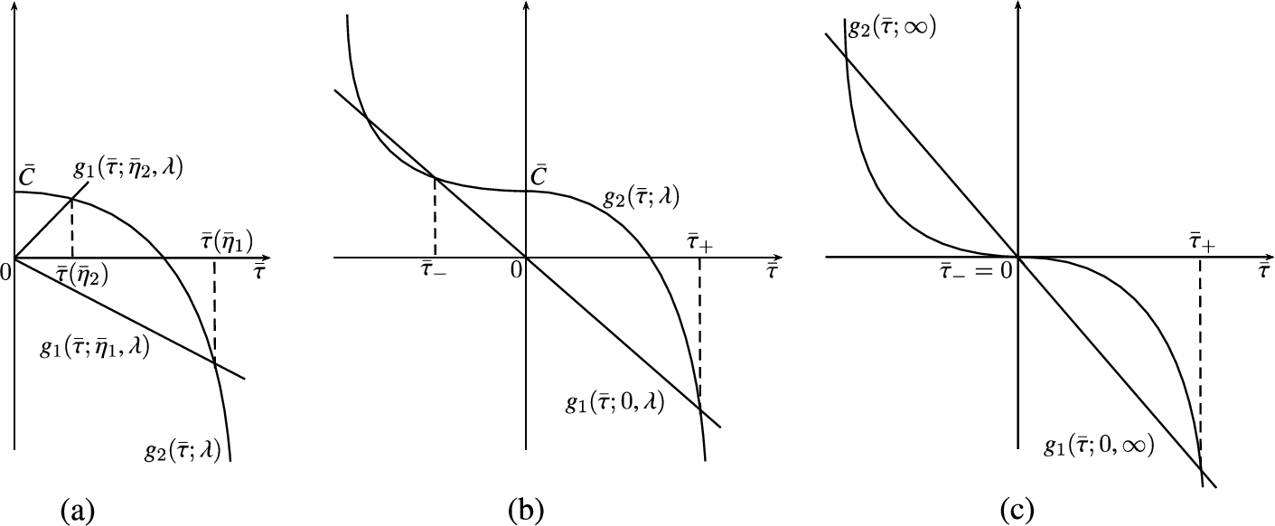
The expression under the “big” radical in (35) is the left-hand side of equation (34) for $\bar{η} = 0$ . Let $\bar{η} = 0$ , then using (23) and passing to the limit $λ \to + \infty$ , from (34) one gets equation $\bar{τ} (1 - \frac{α}{q + 1} {\bar{τ}}^{q}) = 0$ . This equation has at least two real roots: $τ_{-}^{0} = 0$ and $τ_{+}^{0} = {(\frac{q + 1}{α})}^{1 / q}$ . Therefore equation (34) has at least two real roots for $\bar{η} = 0$ and sufficiently large λ. Denote these roots ${\bar{τ}}_{-}$ and ${\bar{τ}}_{+}$ , where ${\bar{τ}}_{+} > 0$ .

It can be proved that ${lim}_{λ \to + \infty} {\bar{τ}}_{-} = τ_{-}^{0}$ and ${lim}_{λ \to \infty} {\bar{τ}}_{+} = τ_{+}^{0}$ . However, the root $τ_{-}$ can be negative, in this case we assume that $τ_{-}$ is the largest of the negative roots. Since $τ = u^{2}$ , the negative values of τ correspond to pure imaginary u. In order to use negative τ, we continue (34) to the domain $\bar{τ} < 0$ .

Below we need asymptotics for ${\bar{τ}}_{-}$ and ${\bar{τ}}_{+}$ for big positive λ. Quantities $τ_{-}^{0}$ and $τ_{+}^{0}$ can be considered as the first approximations to ${\bar{τ}}_{-}$ and ${\bar{τ}}_{+}$ , respectively. Using (23), equality (34) can be rewritten in the form $g_{1} (\bar{τ}; \bar{η}, λ) = g_{2} (\bar{τ}; λ)$ , where $g_{1} (\bar{τ}; \bar{η}, λ) : = ({\bar{η}}^{2} + \bar{a} - 1) \bar{τ}$ , $g_{2} (\bar{τ}; λ) : = {\bar{A}}^{2} - \frac{α}{q + 1} | \bar{τ} |^{q} \bar{τ} - λ^{- 1 - 1 / q} F_{1} (λ^{1 / q} \bar{τ})$ . The module sign is used to continue $g_{2}$ to the domain $\bar{τ} < 0$ . Since in (17) and (35) the integration variable is non-negative, then the modulus sign does not affect calculations for $\bar{τ} ⩾ 0$ . At the same time it allows one to use ${\bar{τ}}_{-}$ . Such a continuation is possible due to dependence of the permittivity ϵ on $| E |^{2}$ , see Section 5.

The function $\bar{τ} (\bar{η}; λ)$ for different $\bar{η}$ is shown in Fig. 1(a); ${\bar{τ}}_{-} \equiv {\bar{τ}}_{-} (λ) < 0$ and ${\bar{τ}}_{+} \equiv {\bar{τ}}_{+} (λ) > 0$ , which are solutions to equation $g_{1} = g_{2}$ for $\bar{η} = 0$ , are shown in Fig. 1(b); case $\bar{η} = 0$ and $λ \to + \infty$ , is demonstrated in Fig. 1(c).

Fig. 1.

Behaviour of $\bar{τ} \equiv \bar{τ} (\bar{η}; λ)$ depending on $\bar{η}$ and λ.

Using (34) for $\bar{η} = 0$ and the approximations found above, one has $\begin{matrix} {\bar{τ}}_{-} = - {\bar{A}}^{2} + O (λ^{- r_{-}}) and {\bar{τ}}_{+} = {(\frac{q + 1}{α})}^{1 / q} + O (λ^{- r_{+}}), \end{matrix}$ where $r_{-} > 1 + 1 / q$ , $r_{+} > 0$ depend on the properties of $F_{1}$ .

Clearly, the “big” radical in (35) vanishes for $\bar{τ} = {\bar{τ}}_{-}$ and $\bar{τ} = {\bar{τ}}_{+}$ ; in addition, ${\bar{τ}}_{-} \to 0$ for $λ \to + \infty$ . Thus there arises a logarithmic singularity at the point $\bar{τ} = 0$ as $λ \to + \infty$ in (35).

The expression under the “big” radical in (35) can be written in the form $\begin{matrix} (36) & {\bar{A}}^{2} + (1 - \bar{a}) \bar{τ} - α λ^{- 1 - 1 / q} F (λ^{1 / q} \bar{τ}) = (\bar{τ} - {\bar{τ}}_{-}) f_{0} (\bar{τ}), \end{matrix}$ where $f_{0} ({\bar{τ}}_{+}) = 0$ and ${lim}_{λ \to + \infty} f_{0} (\bar{τ}) = 1 - \frac{α}{q + 1} | \bar{τ} |^{q}$ . Suppose $g (\bar{τ}) = \frac{1}{\sqrt{f_{0} (\bar{τ})}}$ , then (35) can be rewritten in the form $\begin{matrix} T (λ) = \frac{1}{λ} \int_{0}^{{\bar{τ}}_{+}} \frac{g (\bar{τ}) d \bar{τ}}{\sqrt{\bar{τ} (\bar{τ} - {\bar{τ}}_{-})}} . \end{matrix}$

Let $g_{0} (\bar{τ}) = \frac{1}{\sqrt{{lim}_{λ \to + \infty} f_{0} (\bar{τ})}}$ . Then one has $\begin{matrix} (37) & T = \frac{1}{\sqrt{λ}} \int_{0}^{{\bar{τ}}_{+}} \frac{g (\bar{τ}) d \bar{τ}}{\sqrt{\bar{τ} (\bar{τ} - {\bar{τ}}_{-})}} = \frac{1}{\sqrt{λ}} \int_{0}^{{\bar{τ}}_{+}} \frac{g (\bar{τ}) - g_{0} ({\bar{τ}}_{-})}{\sqrt{\bar{τ} (\bar{τ} - {\bar{τ}}_{-})}} d \bar{τ} + \frac{g_{0} ({\bar{τ}}_{-})}{\sqrt{λ}} \int_{0}^{{\bar{τ}}_{+}} \frac{d \bar{τ}}{\sqrt{\bar{τ} (\bar{τ} - {\bar{τ}}_{-})}} . \end{matrix}$ The first summand in the right-hand side of (37) has the following estimation $\begin{matrix} \int_{0}^{{\bar{τ}}_{+}} \frac{g (\bar{τ}) - g_{0} ({\bar{τ}}_{-})}{\sqrt{\bar{τ} (\bar{τ} - {\bar{τ}}_{-})}} d \bar{τ} = lim_{λ \to + \infty} \int_{0}^{{\bar{τ}}_{+}} \frac{g (\bar{τ}) - g_{0} ({\bar{τ}}_{-})}{\sqrt{\bar{τ} (\bar{τ} - {\bar{τ}}_{-})}} d \bar{τ} + O (λ^{- r_{1}}), \end{matrix}$ where $r_{1} > 0$ . Further, one gets $\begin{array}{rcl} lim_{λ \to + \infty} \int_{0}^{{\bar{τ}}_{+}} \frac{g (\bar{τ}) - g_{0} ({\bar{τ}}_{-})}{\sqrt{\bar{τ} (\bar{τ} - {\bar{τ}}_{-})}} d \bar{τ} & = & \int_{0}^{{(\frac{q + 1}{α})}^{1 / q}} (\frac{1}{\sqrt{1 - \frac{α}{q + 1} {\bar{τ}}^{q}}} - 1) \frac{d \bar{τ}}{\bar{τ}} \\ = & \int_{0}^{{(\frac{q + 1}{α})}^{1 / q}} \frac{\frac{α}{q + 1} {\bar{τ}}^{q - 1}}{\sqrt{1 - \frac{α}{q + 1} {\bar{τ}}^{q}} (1 + \sqrt{1 - \frac{α}{q + 1} {\bar{τ}}^{q}})} d \bar{τ} \\ = & \frac{2}{q} \int_{0}^{1} \frac{d v}{1 + v} = \frac{2 ln 2}{q} . \end{array}$ The second summand in the right-hand side of (37) is calculated exactly and gives $\begin{matrix} \int_{0}^{{\bar{τ}}_{+}} \frac{d \bar{τ}}{\sqrt{\bar{τ} (\bar{τ} - {\bar{τ}}_{-})}} = 2 ln (\sqrt{{\bar{τ}}_{+}} + \sqrt{{\bar{τ}}_{+} - {\bar{τ}}_{-}}) - 2 ln \sqrt{- {\bar{τ}}_{-}} . \end{matrix}$

Now using equations for ${\bar{τ}}_{-}$ and ${\bar{τ}}_{+}$ , one obtains $\begin{array}{l} ln (\sqrt{{\bar{τ}}_{+}} + \sqrt{{\bar{τ}}_{+} - {\bar{τ}}_{-}}) = ln 2 + \frac{1}{2 q} ln \frac{q + 1}{α} + O (λ^{- 1}), \\ ln \sqrt{- {\bar{τ}}_{-}} = - \frac{1}{2} (1 + \frac{1}{q}) ln λ + \frac{1}{2} ln C + O (λ^{- 1}) . \end{array}$ Using (36), one finds $g_{0} ({\bar{τ}}_{-}) = \frac{1}{\sqrt{1 - α | {\bar{τ}}_{-} |^{q}}} = 1 + O (λ^{- 1 - 1 / q})$ .

Finally, uniting the found results, one obtains (24). □

Proof of Theorem 7.

It is clear from (24) that $T (λ) \to 0$ as $λ \to + \infty$ . This yields that there exists an integer $n_{0} ⩾ 0$ such that equation (15) has at least one solution for each $n = n_{0}, n_{0} + 1, \dots$ Thus the problem $P$ has infinitely many positive solutions ${\hat{λ}}_{i}^{+}$ , where ${lim}_{i \to \infty} {\hat{λ}}_{i}^{+} = + \infty$ .

As is seen from (24) the main term of the asymptotic expansion does not depend on α and, therefore, for any $α > 0$ there exists an infinite number of eigenvalues that are not related to any solution of the linear problem.

The asymptotic formula (25) results from (24).

The maximum of $u (x; {\hat{λ}}_{i}^{+})$ can be estimated as follows. Let $u (x; {\hat{λ}}_{i}^{+})$ have at least one zero in the interval $(0, h)$ . There exists a point $x^{*} \in (0, h)$ such that $u^{'} (x^{*}; {\hat{λ}}_{i}^{+}) = 0$ . The required max is equal to $u (x^{*}; {\hat{λ}}_{i}^{+})$ . Well, let $u^{'} = 0$ in (6), one obtains, generally, a transcendental equation. If f satisfies (22), then estimating the maximum root of the found equation, one finds ${max}_{x \in [0, h]} | u (x; \hat{γ}) | = O ({\hat{γ}}^{\frac{1}{2 q}})$ . □

Proof of Theorem 8.

Using equation (24) for the problems $P (q_{1})$ and $P (q_{2})$ , one obtains $T_{j} (λ) = (1 + q_{j}^{- 1}) λ^{- 1 / 2} ln λ + O (λ^{- 1 / 2})$ , where $j = 1, 2$ . This implies that if $q_{1} < q_{2}$ , then $T_{1} > T_{2}$ for a sufficiently big λ and, therefore, ${\hat{λ}}_{1, i} > {\hat{λ}}_{2, i}$ . □

Proof of Statement 10.

It follows from (6), that the first integral of equation (1) can be written in the form $\begin{matrix} (38) & A^{2} - (η^{2} + a - λ) τ + α τ - α (1 + τ) ln (1 + τ) = 0 . \end{matrix}$

From Statement 4 it follows that $Φ (λ; n)$ continuously depends on λ for $λ \in Λ$ . Since $f = ln (1 + u^{2})$ is unbounded, then $λ_{max} = + \infty$ .

Using Statement 7, one has $\begin{matrix} T = \int_{0}^{τ_{+}} \frac{d τ}{\sqrt{τ} \sqrt{A^{2} - (a - λ) τ + α τ - α (1 + τ) ln (1 + τ)}}, \end{matrix}$ where $τ_{+}$ is the positive root of equation (38) for $η = 0$ .

Let us estimate $τ_{+}$ . For this purpose we consider equations $\begin{array}{l} (39) & α (1 + τ) ln (1 + τ) = A^{2} + (λ - a + α) τ, \\ (40) & 2 α τ ln (1 + τ) = (λ - a + α) τ . \end{array}$ Equation (40) has a unique positive root $τ = τ_{min}$ . It is easy to see that $τ_{min} < τ_{+}$ for big τ and λ. From equation (40), one obtains $τ_{min} = exp (\frac{λ - a + α}{2 α}) - 1$ .

Now one can estimate $T (λ)$ . For sufficiently bid λ, one finds $\begin{array}{rcl} T & = & \int_{0}^{τ_{+}} \frac{d τ}{\sqrt{τ} \sqrt{A^{2} - (a - λ) τ + α τ - α (1 + τ) ln (1 + τ)}} \\ ⩾ & \int_{0}^{τ_{+}} \frac{d τ}{\sqrt{τ} \sqrt{A^{2} + (α - a + λ) τ}} ⩾ \int_{0}^{τ_{min}} \frac{d τ}{\sqrt{τ} \sqrt{A^{2} + (α - a + λ) τ}} = T_{min} . \end{array}$ Calculating the integral $T_{min}$ for sufficiently bid values λ, one obtains the estimate $T_{min} = \frac{1}{2 α} λ^{1 / 2} + λ^{- 1 / 2} ln λ + O (λ^{- 1 / 2})$ . From this estimate and the inequality $T ⩾ T_{min}$ , one gets (26). □

Proof of Statement 11.

Estimating function $1 / w (s; λ)$ , one obtains $\begin{matrix} (41) & \frac{π}{\sqrt{a + α f_{max} - λ}} < T (λ) < \frac{π}{\sqrt{a - λ}} . \end{matrix}$ The found estimates result in the estimates given in the statement.

Now let us prove that $Φ (λ; n)$ is not bounded for $λ \to λ_{max}$ . Let $δ^{'} > 0$ be a fixed sufficiently small number. Equation (15) always contains the term $\begin{matrix} \int_{0}^{δ^{'}} \frac{d s}{w (s; λ)} . \end{matrix}$

Let $U_{λ_{max}}$ be a sufficiently small half-neighbourhood (on the real axis $R$ ) of the point $λ_{max}$ . Let us consider equation (10) for $s \in [0, δ]$ and $λ \in U_{λ_{max}}$ . Clearly, solution $τ \equiv τ (s; λ)$ to equation (10) exists for $λ \in U_{λ_{max}}$ . From the proof of Statement 3 it follows that for sufficiently small $δ^{'}$ the solution $τ (s; λ)$ satisfies the inequality $τ (s; λ) ⩽ τ_{+}$ , where $τ_{+}$ is a sufficiently big constant. Well, $f (s) ⩽ f (τ_{+})$ , where the smaller $δ^{'}$ and $U_{λ_{max}}$ are, the smaller $| f (τ_{+}) - f_{max} |$ is.

Clearly, the following estimates $\begin{matrix} \int_{0}^{δ^{'}} \frac{d s}{s^{2} + a - λ + α f (τ_{+})} ⩽ \int_{0}^{δ^{'}} \frac{d s}{w (s; λ)} \end{matrix}$ take place. Let $r (s) : = \sqrt{a - λ + α f (s)}$ . Calculating the integral on the left-hand side, one gets $\begin{matrix} \frac{1}{r (τ_{+})} arctan \frac{δ^{'}}{r (τ_{+})} ⩽ \int_{0}^{δ^{'}} \frac{d s}{w (s; λ)} . \end{matrix}$

If $λ \to - δ^{'} + a + α f (τ_{+})$ , then $\frac{δ^{'}}{r (τ_{+})} \to 1$ . This result does not depend on $δ^{'}$ . However, if $δ^{'} \to 0$ , then $f (τ_{+}) \to f_{max}$ and, therefore, $r (τ_{+}) \to 0$ . This implies that the left-hand side of the inequality obtained above tends to infinity as $λ \to a + α f_{max}$ . Thus ${lim}_{λ \to λ_{max}} Φ (λ; n) = + \infty$ . □

Footnotes

Acknowledgements

The authors thank the reviewers for their careful reading of the manuscript and the valuable comments and remarks which improved the final version of the original manuscript. This research was supported by the Russian Science Foundation, under the grant 18-71-10015.

References

M.J.

Adams, An Introduction to Optical Waveguides, John Wiley & Sons, Chichester, New York–Brisbane–Toronto, 1981.

N.N.

Akhmediev and

Ankevich, Solitons, Nonlinear Pulses and Beams, Chapman and Hall, London, 1997.

S.J.

Al-Bader and

H.A.

Jamid, Nonlinear waves in saturable self-focusing thin films bounded by linear media, IEEE Journal of Quantum Electronics 24(10) (1988), 2052–2058. doi:10.1109/3.8541.

Ambrosetti and

P.H.

Rabinowitz, Dual variational methods in critical point theory and applications, Journal of Functional Analysis 14(4) (1973), 349–381. doi:10.1016/0022-1236(73)90051-7.

W.O.

Amrein,

A.M.

Hinz and

D.B.

Pearson, Sturm–Liouville Theory: Past and Present, Birkhäuser Verlag, Basel/Switzerland, 2005.

R.D.

Benguria,

M.C.

Depassier and

Loss, Monotonicity of the period of a non linear oscillator, Nonlinear Analysis 140 (2016), 61–68. doi:10.1016/j.na.2016.03.004.

Yu.N.

Bibikov, Course of Ordinary Differential Equations, “Vysshaya Shkola”, Moscow, 1991 (in Russian).

A.D.

Boardman,

Egan,

Lederer,

Langbein and

Mihalache, Third-Order Nonlinear Electromagnetic TE and TM Guided Waves, Elsevier Sci. Publ., North-Holland, Amsterdam London, New York, Tokyo, 1991 (Reprinted from Nonlinear Surface Electromagnetic Phenomena, H.-E. Ponath and G.I. Stegeman, Eds.).

R.F.

Brown, A Topological Introduction to Nonlinear Analysis, 2nd edn, Springer, 2004.

10.

Cazenave, Semilinear Schrödinger Equations, Courant Lecture Notes in Mathematics, Vol. 10, American Mathematical Society, 2003.

11.

Feltrina and

Zanolin, Multiple positive solutions for a superlinear problem: A topological approach, Journal of Differential Equations 259(3) (2015), 925–963. doi:10.1016/j.jde.2015.02.032.

12.

I.Tz.

Gokhberg and

M.G.

Krein, Introduction in the Theory of Linear Nonselfadjoint Operators in Hilbert Space, Amer. Math. Soc., 1969.

13.

Hartman, Ordinary Differential Equations, John Wiley & Sons, 1964.

14.

Kamke, Differentialgleichungen. Lösungmethoden und Lösungen. Gewönliche Differentialgleichungen, Akademische Verlagsgesellschaft Geest & Portig K.-G., Leipzig, 1959.

15.

Kato, Perturbation Theory for Linear Operators, Springer, Heidelberg, 1966.

16.

J.B.

Keller and

Antman (eds), Bifurcation Theory and Nonlinear Eigenvalue Problems, W. A. Benjamin, Inc., 1969.

17.

M.A.

Krasnosel’skii, Topological Methods in the Theory of Nonlinear Integral Equations, Pergamon Press, Oxford–London, New York–Paris, 1964.

18.

V.Yu.

Kurseeva,

S.V.

Tikhov and

D.V.

Valovik, Nonlinear multiparameter eigenvalue problems: Linearised and nonlinearised solutions, Journal of Differential Equations 267(4) (2019), 2357–2384. doi:10.1016/j.jde.2019.03.014.

19.

L.D.

Landau,

E.M.

Lifshitz and

L.P.

Pitaevskii, Course of Theoretical Physics (Vol. 8). Electrodynamics of Continuous Media, Butterworth-Heinemann, Oxford, 1993.

20.

V.A.

Marchenko, Sturm–Liouville Operators and Applications. Operator Theory: Advances and Applications, Springer, Basel AG, 1986.

21.

A.S.

Markus, Introduction to the Spectral Theory of Polynomial Operator Pencils, AMS, Providence, Rhode Island, 1988.

22.

A.I.

Markushevich, Theory of Functions of a Complex Variable, AMS, Providence, Rhode Island, 2011.

23.

J.L.

Massera, The existence of periodic solutions of systems of differential equations, Duke Mathematical Journal 17(4) (1950), 457–475. doi:10.1215/S0012-7094-50-01741-8.

24.

Nehari, Characteristic values associated with a class of nonlinear second-order differential equations, Acta Mathematica 105(3–4) (1961), 141–175. doi:10.1007/BF02559588.

25.

V.G.

Osmolovskii, Nonlinear Sturm–Liouville Problem, Saint Petersburg University Press, Saint Petersburg, Russia, 2003.

26.

I.G.

Petrovsky, Lectures on the Theory of Ordinary Differential Equations, Moscow State University, Moscow, 1984 (in Russian).

27.

Reissig,

Sansone and

Conti, Qualitative Theorie Nichtlinearer Differentialgleichungen, Edizioni Cremonese, Roma, 1963.

28.

H.W.

Schürmann,

Yu.G.

Smirnov and

Yu.V.

Shestopalov, Propagation of te-waves in cylindrical nonlinear dielectric waveguides, Phys. Rev. E 71(1) (2005), 016614(10).

29.

Y.R.

Shen, The Principles of Nonlinear Optics, John Wiley and Sons, New York–Chicester–Brisbane–Toronto–Singapore, 1984.

30.

Shibata, New asymptotic formula for eigenvalues of nonlinear Sturm–Liouville problems, Journal d’Analyse Mathématique 102(1) (2007), 347–358. doi:10.1007/s11854-007-0024-y.

31.

Struwe, Multiple solutions of anticoercive boundary value problems for a class of ordinary differential equations of second order, Journal of Differential Equations 37(2) (1980), 285–295. doi:10.1016/0022-0396(80)90099-6.

32.

S.V.

Tikhov and

D.V.

Valovik, Perturbation of nonlinear operators in the theory of nonlinear multifrequency electromagnetic wave propagation, Communications in Nonlinear Science and Numerical Simulation 75 (2019), 76–93. doi:10.1016/j.cnsns.2019.03.020.

33.

F.G.

Tricomi, Differential Equations, Blackie & Son Limited, New York, 1961.

34.

M.M.

Vainberg, Variational Methods for the Study of Nonlinear Operators, 1st edn, Holden-Day Series in Mathematical Physics. Holden-Day, 1964.

35.

D.V.

Valovik, Novel propagation regimes for te waves guided by a waveguide filled with Kerr medium, Journal of Nonlinear Optical Physics & Materials 25(4) (2016), 1650051 (17).

36.

D.V.

Valovik, On a nonlinear eigenvalue problem related to the theory of propagation of electromagnetic waves, Differential Equations 54(2) (2018), 168–179. doi:10.1134/S0012266118020039.

37.

D.V.

Valovik, On spectral properties of the Sturm–Liouville operator with power nonlinearity, Monatshefte für Mathematik 188(2) (2019), 369–385. doi:10.1007/s00605-017-1124-0.

38.

D.V.

Valovik and

V.Yu.

Kurseeva, On the eigenvalues of a nonlinear spectral problem, Differential Equations 52(2) (2016), 149–156. doi:10.1134/S0012266116020026.

39.

P.E.

Zhidkov, Riesz basis property of the system of eigenfunctions for a non-linear problem of Sturm–Liouville type, Sbornik: Mathematics 191(3) (2000), 359–368. doi:10.1070/SM2000v191n03ABEH000461.