Weakly nonlinear surface waves in magnetohydrodynamics. I

Abstract

This work is devoted to the construction of weakly nonlinear, highly oscillating, current vortex sheet solutions to the system of ideal incompressible magnetohydrodynamics. Current vortex sheets are piecewise smooth solutions that satisfy suitable jump conditions on the (free) discontinuity surface. In this article, we complete an earlier work by Alì and Hunter (Quart. Appl. Math. 61(3) (2003) 451–474) and construct approximate solutions at any arbitrarily large order of accuracy to the three-dimensional free boundary problem when the initial discontinuity displays high frequency oscillations. As evidenced in earlier works, high frequency oscillations of the current vortex sheet give rise to ‘surface waves’ on either side of the sheet. Such waves decay exponentially in the normal direction to the current vortex sheet and, in the weakly nonlinear regime which we consider here, their leading amplitude is governed by a nonlocal Hamilton–Jacobi type equation known as the ‘HIZ equation’ (standing for Hamilton–Il’insky–Zabolotskaya (J. Acoust. Soc. Amer. 97(2) (1995) 891–897)) in the context of Rayleigh waves in elastodynamics.

The main achievement of our work is to develop a systematic approach for constructing arbitrarily many correctors to the leading amplitude. We exhibit necessary and sufficient solvability conditions for the corrector equations that need to be solved iteratively. The verification of these solvability conditions is based on mere algebra and arguments of combinatorial analysis, namely a Leibniz type formula which we have not been able to find in the literature. The construction of arbitrarily many correctors enables us to produce infinitely accurate approximate solutions to the current vortex sheet equations. Eventually, we show that the rectification phenomenon exhibited by Marcou in the context of Rayleigh waves (C. R. Math. Acad. Sci. Paris 349(23–24) (2011) 1239–1244) does not arise in the same way for the current vortex sheet problem.

Keywords

Magnetohydrodynamics current-vortex sheet weakly nonlinear analysis surface waves WKB expansion stability

1. Introduction and main result

1.1. Motivation

This work is devoted to the asymptotic analysis of a free boundary problem arising in magnetohydrodynamics (MHD), namely the current vortex sheet problem. We consider a homogeneous, perfectly conducting, inviscid and incompressible plasma. The model consists of the so-called ideal incompressible MHD system, which reads in dimensionless form: $\begin{matrix} (1) & \{\begin{matrix} \partial_{t} u + \nabla \cdot (u \otimes u - H \otimes H) + \nabla q = 0, \\ \partial_{t} H - \nabla \times (u \times H) = 0, \\ \nabla \cdot u = \nabla \cdot H = 0 . \end{matrix} \end{matrix}$ In (1), $u \in R^{3}$ and $H \in R^{3}$ respectively stand for the velocity and the magnetic field of the plasma, × denotes the cross product in $R^{3}$ and $\nabla \cdot$ , resp. ∇, denotes the divergence, resp. gradient, operator with respect to the three-dimensional space variable $x = (x_{1}, x_{2}, x_{3})$ . The scalar unknown $q : = p + | H |^{2} / 2$ is the ‘total’ pressure, p being the ‘physical’ pressure.

We are interested here in a special class of weak solutions to (1): we want $(u, H, q)$ to be smooth, for each time t, on either side of a hypersurface $Γ (t) \subset R^{3}$ , and to give rise to a tangential discontinuity across $Γ (t)$ . The appropriate jump conditions (2) on $Γ (t)$ are described below. For simplicity, we shall assume that the hypersurface $Γ (t)$ is a graph that can be parametrized by $Γ (t) = {x \in R^{3} / x_{3} = ψ (t, x^{'})}$ for some smooth function ψ of $(t, x^{'})$ to be determined, with $x^{'} : = (x_{1}, x_{2})$ the tangential space variable which we shall consider to be lying in the two-dimensional torus $T^{2} : = R^{2} / (2 π Z^{2})$ . The unknown ψ that parametrizes Γ will be called the ‘front’ of the discontinuity later on. We shall thus consider the incompressible MHD system (1) in the time-dependent domain: $\begin{matrix} Ω (t) : = Ω^{+} (t) ⊔ Ω^{-} (t), where Ω^{\pm} (t) : = {x_{3} ≷ ψ (t, x^{'})}, \end{matrix}$ with the following jump conditions on $Γ (t)$ (the superscripts ± denote the trace on $Γ (t)$ from each subdomain $Ω^{\pm} (t)$ ): $\begin{matrix} (2) & \partial_{t} ψ = u^{+} \cdot N = u^{-} \cdot N, H^{+} \cdot N = H^{-} \cdot N = 0, [q] = 0 . 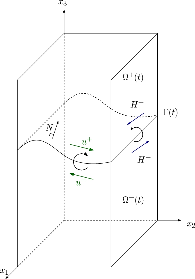\end{matrix}$ The notation $[q]$ in (2) stands for the jump of the total pressure q across $Γ (t)$ : $\begin{matrix} [q] : = q^{+} |_{Γ (t)} - q^{-} |_{Γ (t)}, \end{matrix}$ and the notation N in (2) stands for the normal vector to $Γ (t)$ chosen as follows (the superscript T stands for transposition): $\begin{array}{l} N : = {(- \partial_{x_{1}} ψ, - \partial_{x_{2}} ψ, 1)}^{T} . \end{array}$

The boundary conditions (2) correspond to a tangential discontinuity. The velocity $\partial_{t} ψ$ of the front is given by the normal component of the fluid velocity on either side of the free discontinuity, meaning that the fluid does not flow through the interface $Γ (t)$ . The normal magnetic field $H^{\pm} \cdot N$ is zero (hence continuous) on either side of the discontinuity, and the total pressure $q^{\pm}$ should also be continuous across $Γ (t)$ . Such boundary conditions account for the evolution of a plasma which gives rise to a current vortex sheet (see, e.g., Fig. 1 below). Both $\nabla \times u$ and $\nabla \times H$ have a singular component on $Γ (t)$ . We refer to [12,14] for other types of discontinuities in compressible or incompressible MHD.

Fig. 1.

Schematic picture of a current vortex sheet.

To be consistent with several earlier works on current vortex sheets [15,33,39], we shall assume that the plasma is confined in the strip $x_{3} \in (- 1, 1)$ . In particular, the front ψ should satisfy $- 1 < ψ (t, x^{'}) < 1$ for all $(t, x^{'})$ so that the current vortex sheet itself is located within the strip. We then impose the standard boundary conditions on the fixed ‘top’ and ‘bottom’ boundaries $Γ^{\pm} : = {(x^{'}, \pm 1), x^{'} \in T^{2}}$ . On $Γ^{\pm}$ , the plasma should have zero normal velocity and zero normal magnetic field. In its quasilinear form, the system of current vortex sheets eventually reads as follows: $\begin{matrix} (3) & \{\begin{matrix} \partial_{t} u^{\pm} + (u^{\pm} \cdot \nabla) u^{\pm} - (H^{\pm} \cdot \nabla) H^{\pm} + \nabla q^{\pm} = 0, & in Ω^{\pm} (t), t \in [0, T], \\ \partial_{t} H^{\pm} + (u^{\pm} \cdot \nabla) H^{\pm} - (H^{\pm} \cdot \nabla) u^{\pm} = 0, & in Ω^{\pm} (t), t \in [0, T], \\ \nabla \cdot u^{\pm} (t) = \nabla \cdot H^{\pm} (t) = 0, & in Ω^{\pm} (t), t \in [0, T], \\ \partial_{t} ψ = u^{\pm} \cdot N, H^{\pm} \cdot N = 0, [q] = 0, & on Γ (t), t \in [0, T], \\ u_{3}^{\pm} = H_{3}^{\pm} = 0, & on [0, T] \times Γ^{\pm} . \end{matrix} \end{matrix}$ The superscripts ± in (3) refer to the restriction of the unknowns u, H and q to the subdomains $Ω^{\pm} (t)$ . Of course, (3) should be supplemented with initial conditions for $ψ, u^{\pm}, H^{\pm}$ that satisfy suitable compatibility requirements (e.g., the divergence free constraints in (3) and the boundary conditions on $Γ^{\pm}$ ).

The local in time solvability of (3) in Sobolev spaces has been recently proved by Sun, Wang and Zhang [39] by a clever reduction to the free boundary in the spirit of water wave theory. This reduction yields a second order scalar hyperbolic equation for the front ψ, a linearized version of which will play a crucial role in our analysis. The well-posedness result of [39] relies on a stability condition that dates back, at least, to [5,40] and that also plays a crucial role in the present analysis. An alternative approach to [39], which does not rely on any stability condition but that is restricted to analytic data, has been recently proposed by the first author [33] with the aim of extending it to in the compressible case. Within this article, we are interested in the qualitative behavior of exact solutions to (3) for highly oscillating initial data. This problem has been addressed by Alì and Hunter [1] who have considered the two-dimensional problem and who have shown that for some specific oscillation phase, and in the weakly nonlinear regime, the leading amplitude of the solution on either side of the current vortex sheet displays a surface wave structure: it oscillates with the same phase as the front and is exponentially localized near the free surface. Such a phenomenon is entirely analogous to the description of weakly nonlinear Rayleigh waves in elastodynamics, see, e.g., [18,24,25,31,32] and further references therein.

That surface waves occur in the current vortex sheet problem can be explained by performing a so-called normal mode analysis. Given a reference piecewise constant solution to the current vortex sheet system (3), we seek for plane waves of the form $exp (i (τ t + ξ_{1} x_{1} + ξ_{2} x_{2} + ξ_{3} x_{3}))$ , with $τ \in C$ , $(ξ_{1}, ξ_{2}) \in R^{2}$ and $ξ_{3} \in C$ , which can be solutions to the linearization of (3) at the given piecewise constant solution. Here, the normal coordinate to the (flat) sheet is $x_{3}$ . Due to the divergence-free constraints on the velocity and the magnetic field, the resulting system is not a ‘standard’ hyperbolic system. However, the method we use is analogous to the case of free boundary hyperbolic problems [11]: the goal is to verify whether the weak and/or the uniform Kreiss–Lopatinskii condition [23] (ULC for short hereafter) is satisfied in order to obtain a linear stability criterion for planar current vortex sheets. The analysis of the linearized problem performed in [5,14,40], and more recently in [30], leads to a necessary stability criterion by eliminating the case $Im τ < 0$ for which the normal modes blow up (the problem would then typically be strongly ill-posed unless the data are analytic). The limit ‘neutral’ case we are interested in corresponds to $Im τ = 0$ ; we shall say that the problem is weakly well-posed. Weak well-posedness is associated with real frequencies $(τ, ξ_{1}, ξ_{2}) \in R^{3}$ for which the so-called Lopatinskii determinant vanishes. For the current vortex sheet problem (3), only the weak Lopatinskii condition is fulfilled at best, meaning that there does not exist any planar current vortex sheet for which the ULC is satisfied. We refer for instance to [30] for more details. The main, striking, result of [39] shows that the linear stability criterion that precludes violent instabilities is actually a sufficient condition for nonlinear stability in the Sobolev regularity scale.

In our problem, the roots $(τ, ξ_{1}, ξ_{2}) \in R^{3}$ of the Lopatinskii determinant can be parametrized by $(ξ_{1}, ξ_{2})$ . Namely, under the linear stability condition which we shall recall below, for any fixed tangential frequency $(ξ_{1}, ξ_{2}) \in R^{2} ∖ {0}$ , there exist two simple roots $τ_{\pm} (ξ_{1}, ξ_{2})$ of the Lopatinskii determinant, and these roots belong to the set of so-called elliptic frequencies because the corresponding normal frequency $ξ_{3}$ is not real (it is even a purely imaginary number). Those frequencies are responsible for the creation of surface waves, which corresponds to the case $Im ξ_{3} ≷ 0$ (depending on the sign of $x_{3}$ ). Surface waves decay exponentially with respect to $x_{3}$ . In other problems related to hydrodynamics, such as detonation waves or compressible vortex sheets [3,27], the normal frequency $ξ_{3}$ associated with the roots of the Lopatinskii determinant is real, which gives rise to bulk waves that radiate into the whole domain, see [10] for a general description of this class of problems. The latter case does not arise when studying current vortex sheets in incompressible MHD. At the opposite, the MHD problem we consider here is closer to the one studied by Sablé–Tougeron [36] whose prototype example is the system of elastodynamics with zero normal stress on the boundary (which gives rise to the so-called Rayleigh waves). Another occurrence of surface waves in MHD is the so-called plasma-vacuum interface problem [37,38].

The main question we address here follows a long line of research, whose rigorous mathematical formulation dates back to Hunter [19], see also [2,4,9,16,28,43], and is concerned with the evolution of weakly nonlinear surface waves. Up to a time rescaling, we shall be concerned with the slow modulation of high frequency, small amplitude surface wave solutions to (3). We follow the seminal work of Alì and Hunter [1] with two main extensions; not only do we consider the three dimensional case to the price of some more algebra (the analysis in [1] is performed in two space dimensions), but what is more significant is that we give a complete construction of infinitely accurate solutions to (3) in the high frequency limit (the analysis in [1] is more or less restricted to the construction of the leading order amplitude). This is done by enlightening several algebraic properties in the analysis of the WKB cascade, some of which might be useful in other contexts. The construction of arbitrarily many correctors is not a mere technical issue. It is a crucial step towards the rigorous justification that exact solutions to (3) with highly oscillating data are actually close to the WKB expansion we shall construct here, see, e.g., [17,21,28,35,43]. However, we do not address this stability problem because of intricate nonlocality issues [39], and rather focus on the construction of a solution to the WKB cascade.

In the following paragraphs of this introduction, we present our main result by first stating the assumptions on the reference planar current vortex sheet and on the frequencies we shall work with. We then introduce the functional framework in which we shall solve the WKB cascade that will be made explicit in Section 2. Eventually we state our main result and give the plan for its proof. Due to editorial constraints, we only give in this article a detailed plan of the proof of our main result, which is Theorem 1.2 below. All complementary details of the proof are given in the companion article [34] that is available at: https://dx-doi-org.web.bisu.edu.cn/10.3233/ASY-201638.

1.2. Choice of parameters and initial data for the front

Our goal is to construct highly oscillating solutions to (3) that are small perturbations of a reference piecewise constant solution to (3). The starting point is to fix the reference current vortex sheet. By imposing a suitable stability condition, inequality (H1) below, this will enable us to fix the planar phase of the oscillations for the front. The goal will then be to describe the behavior of the solution to (3) on either side of the oscillating front by choosing (and hopefully one day justifying) a suitable WKB ansatz. As a long term goal, this will justify the asymptotic behavior of the exact solution to (3) when we impose highly oscillating initial data. In particular, part of our work aims at justifying that for suitably chosen oscillating initial data, the exact solution to (3) exists on a time interval that is independent of the small wavelength of the initial oscillations.

1.2.1. The reference current vortex sheet

To be consistent with the notation below for the WKB ansatz, we consider a (steady) piecewise constant solution to (3) of the form $\begin{matrix} (4) & U^{\pm} (t, x) = \{\begin{matrix} U^{0, +}, & if x_{3} \in (0, 1), \\ U^{0, -}, & if x_{3} \in (- 1, 0), \end{matrix} \end{matrix}$ where the two constant states $U^{0, \pm}$ , and the corresponding fixed reference front1

¹
We use two functions $ψ^{0}$ and $ψ^{1}$ since the leading front should be rather thought of as $ψ^{0} + ε ψ^{1}$ . One possible extension of our work would be to study high frequency oscillations on a curved current vortex sheet. In that case, both $ψ^{0}$ and $ψ^{1}$ would be nontrivial.

ψ^{0}, ψ^{1}

, are given by:

\begin{matrix} (5) & U^{0, \pm} : = {(u_{1}^{0, \pm}, u_{2}^{0, \pm}, 0, H_{1}^{0, \pm}, H_{2}^{0, \pm}, 0, 0)}^{T}, ψ^{0}, ψ^{1} : = 0 . \end{matrix}

Here and from now on, the notation U stands for a column vector in

R^{7}

whose coordinates are labeled

u_{1}, u_{2}, u_{3}, H_{1}, H_{2}, H_{3}, q

. The normalization of the total pressure

q^{0, \pm} = 0

in (5) is consistent with the choice that is made below for the solution to (3), namely:2

Recall the jump condition $[q] = 0$ in (3) across the interface $Γ (t)$ , so the total pressure in $Ω^{+} (t) \cup Ω^{-} (t)$ is defined up to a single function of time only.

\begin{matrix} \int_{Ω^{+} (t)} q^{+} (t, x) d x + \int_{Ω^{-} (t)} q^{-} (t, x) d x = 0 . \end{matrix}

For later use, we assume that the reference current vortex sheet (5) fulfills the following stability criterion:

\begin{matrix} (H1) & {| H^{0, +} \times [u^{0}] |}^{2} + {| H^{0, -} \times [u^{0}] |}^{2} < 2 {| H^{0, +} \times H^{0, -} |}^{2}, \end{matrix}

where

[u^{0}] : = u^{0, +} - u^{0, -}

stands for the jump of the velocity

u^{0}

across the flat sheet

{x_{3} = 0}

. The stability condition (H1) has been highlighted in [5,14,40] and more recently in [30,39]. A restricted version of (H1) is used in [15,41].

1.2.2. The frequencies

Let us begin with a few notations. The $2 π$ -periodic torus $R / (2 π Z)$ is denoted by $T$ and the tangential spatial variable is $x^{'} = (x_{1}, x_{2}) \in T^{2}$ . We consider a given tangential frequency vector $ξ^{'} = (ξ_{1}, ξ_{2}) \in R^{2}$ which we normalize by assuming $| ξ^{'} | : = \sqrt{ξ_{1}^{2} + ξ_{2}^{2}} = 1$ . We also choose a real time frequency τ which will be assumed to meet several requirements below, but let us right away define the planar phase $τ t + ξ^{'} \cdot x^{'}$ , the notation · referring to the inner product of $R^{2}$ . With the reference planar current vortex sheet defined by (5), we define the following parameters: $\begin{matrix} (6) & a^{\pm} : = ξ_{1} u_{1}^{0, \pm} + ξ_{2} u_{2}^{0, \pm}, b^{\pm} : = ξ_{1} H_{1}^{0, \pm} + ξ_{2} H_{2}^{0, \pm}, c^{\pm} : = τ + a^{\pm} . \end{matrix}$

Given a $2 π$ -periodic function $v = v (x^{'}, θ)$ with respect to each of its arguments $(x^{'}, θ) \in T^{3}$ , we shall require below that the function: $\begin{matrix} v_{ε} (x^{'}) : = v (x^{'}, \frac{ξ^{'} \cdot x^{'}}{ε}), \end{matrix}$ be $2 π$ -periodic with respect to $x^{'}$ . To do so, we need to impose some additional conditions on the frequency vector $ξ^{'}$ . We choose the frequency $ξ^{'}$ of the form: $\begin{matrix} (H2) & ξ^{'} = \frac{1}{\sqrt{p^{2} + q^{2}}} {(p, q)}^{T} with {(p, q)}^{T} \in Z^{2} ∖ {0} . \end{matrix}$ Then, considering the sequence ${(ε_{ℓ})}_{ℓ ⩾ 1}$ defined by: $\begin{matrix} (7) & ε_{ℓ} : = \frac{1}{ℓ \sqrt{p^{2} + q^{2}}}, ℓ ⩾ 1, \end{matrix}$ which tends to 0 as ℓ goes to $+ \infty$ , we will indeed have $ξ^{'} / ε_{ℓ} \in Z^{2}$ and therefore the above function $v_{ε_{ℓ}}$ will be $2 π$ -periodic with respect to $x^{'}$ for any integer $ℓ ⩾ 1$ . In the following, the frequency vector $ξ^{'}$ is chosen of the form (H2) and the small parameter ε stands for one element of the sequence ${(ε_{ℓ})}_{ℓ ⩾ 1}$ in (7). When we write $ε \to 0$ , we mean that we consider $ε_{ℓ}$ with $ℓ \to + \infty$ .

We add another assumption on the frequency $ξ^{'}$ in order to fulfill the technical condition ${(c^{\pm})}^{2} \neq {(b^{\pm})}^{2}$ used in the proof of our main result, see the companion article [34] for more details: $\begin{matrix} (H3) & \{\begin{matrix} | a^{+} - a^{-} | \neq | b^{+} - b^{-} |, \\ | a^{+} - a^{-} | \neq | b^{+} + b^{-} | . \end{matrix} \end{matrix}$ In other words, if we define the following three vectors in $R^{2}$ : $\begin{matrix} u : = (u_{1}^{0, +} - u_{1}^{0, -}, u_{2}^{0, +} - u_{2}^{0, -}), h_{\pm} : = (H_{1}^{0, +} \pm H_{1}^{0, -}, H_{2}^{0, +} \pm H_{2}^{0, -}), \end{matrix}$ then we ask the frequency $ξ^{'}$ not to be orthogonal to the four vectors $u - h_{+}$ , $u - h_{-}$ , $u + h_{+}$ , $u + h_{-}$ . None of these four vectors is zero because of Assumption (H1). Indeed, if we have for instance $u = h_{-}$ , then it would lead to the identity $[u^{0}] = [H^{0}]$ , and plugging this equality into (H1), we would obtain: $\begin{matrix} 2 {| H^{0, +} \times H^{0, -} |}^{2} < 2 {| H^{0, +} \times H^{0, -} |}^{2}, \end{matrix}$ which is a contradiction. The same argument applies for the three remaining cases. Choosing $ξ^{'}$ of the form (H2) and satisfying (H3) is possible because satisfying (H3) amounts to excluding at most four directions on the unit circle $S^{1}$ and unit vectors of the form (H2) are dense in $S^{1}$ .

Given $ξ^{'} \in R^{2}$ satisfying (H2) and (H3), it remains to make the restrictions on the time frequency τ explicit. In all what follows, we choose the time frequency $τ \in R$ as one (among the two) root(s) of the so-called Lopatinskii determinant. Referring to [30] for the computation of the latter quantity, see also [34], we choose τ as a root to the following polynomial equation of degree 2 (recall the definition (6)): $\begin{matrix} (H4) & {(c^{+})}^{2} + {(c^{-})}^{2} = {(b^{+})}^{2} + {(b^{-})}^{2} . \end{matrix}$ That Assumption (H1) on the reference planar current vortex sheet implies that (H4) has two real simple roots follows from elementary algebraic considerations, see [15,30,34].

The last requirement on the time frequency is the assumption $τ \neq 0$ . The relevance of this last assumption is justified in the companion article [34] where we use it to parametrize some eigenspaces. Let us just observe that the condition $τ \neq 0$ automatically follows from (H4) if $u_{0}^{+} + u_{0}^{-} = 0$ (in that case $a^{+} = - a^{-}$ ), which can always be achieved by using the Galilean invariance of system (3). Assumptions (H2), (H3), (H4) and the condition $τ \neq 0$ allow to ensure ${(c^{\pm})}^{2} \neq {(b^{\pm})}^{2}$ , see [34], which will turn out to be crucial in the analysis of the WKB cascade.

From now on, the reference planar current vortex sheet (4) and the frequencies $(τ, ξ_{1}, ξ_{2}) \in R^{3}$ satisfying Assumptions (H1), (H2), (H3), (H4), together with $τ \neq 0$ , are fixed. We now describe the oscillating data that we consider for the system (3).

1.2.3. Initial data for the front and WKB ansatz

We consider small, highly oscillating perturbations of the reference constant state $(U^{0, \pm}, ψ^{0} + ε ψ^{1})$ . To be specific, we shall consider initial data for the front of the form: $\begin{matrix} (8) & ψ_{ε} (t = 0, x^{'}) : = ε^{2} ψ_{0}^{2} (x^{'}, \frac{ξ^{'} \cdot x^{'}}{ε}), \end{matrix}$ where the initial profile $ψ_{0}^{2} \in C^{\infty} (T^{3})$ is assumed to have zero mean with respect to its last argument $θ \in T$ . Let us recall that the small parameter $ε \in (0, 1]$ actually stands for any $ε_{ℓ}$ defined by (7) so that $ψ_{ε}$ in (8) is indeed $2 π$ -periodic with respect to $x^{'}$ . We could consider a sequence of profiles $ψ_{0}^{2}, ψ_{0}^{3}, \dots$ and the corresponding initial condition: $\begin{matrix} ψ_{ε} (t = 0, x^{'}) = ε^{2} ψ_{0}^{2} (x^{'}, \frac{ξ^{'} \cdot x^{'}}{ε}) + ε^{3} ψ_{0}^{3} (x^{'}, \frac{ξ^{'} \cdot x^{'}}{ε}) + \dots, \end{matrix}$ the series in ε being either convergent or understood as an asymptotic expansion, but this would not add any new phenomenon nor any analytical difficulty; we therefore restrict to the initial datum (8) for notational convenience. Choosing the initial profile $ψ_{0}^{2}$ to have zero mean with respect to θ is also done for the sake of convenience. In any case, the mean of $ψ_{0}^{2}$ with respect to θ will not affect the leading amplitude of the solution on either side of the current vortex sheet.

The initial front $ψ_{ε} |_{t = 0}$ will take its values in the strip $(- 1, 1)$ up to restricting ε if necessary. Since ε is meant to be small, we shall not go back to this issue any longer.

Continuing the analysis of [1], we seek an asymptotic expansion of the exact solution $(U_{ε}^{\pm}, ψ_{ε})$ to (3) as a small, highly oscillating perturbation of the reference planar current vortex sheet (5). Some attention needs to be paid when formulating the WKB ansatz for $(U_{ε}^{\pm}, ψ_{ε})$ . The front $ψ_{ε}$ is meant to oscillate with the planar phase $τ t + ξ^{'} \cdot x^{'}$ with a slow modulation in the tangential variables $(t, x^{'})$ . The interior solution $U_{ε}^{\pm}$ will display oscillations with the same planar phase $τ t + ξ^{'} \cdot x^{'}$ , and exponential decay with respect to the fast normal variable $(x_{3} - ψ_{ε} (t, x^{'})) / ε$ . However, describing the modulation of $U_{ε}^{\pm}$ also requires taking into account the slow normal variable $x_{3} - ψ_{ε} (t, x^{'})$ and the fixed top and bottom boundaries $Γ^{\pm}$ too. We thus introduce once and for all a fixed cut-off function $χ \in C^{\infty} (R)$ such that $χ \equiv 1$ on $[- 1 / 3, 1 / 3]$ and χ vanishes outside of $[- 2 / 3, 2 / 3]$ . We aim at constructing an asymptotic expansion for $(U_{ε}^{\pm}, ψ_{ε})$ of the following form: $\begin{array}{l} (9a) & U_{ε}^{\pm} (t, x) \sim U^{0, \pm} + \sum_{m ⩾ 1} ε^{m} U^{m, \pm} (t, x^{'}, x_{3} - χ (x_{3}) ψ_{ε} (t, x^{'}), \frac{x_{3} - ψ_{ε} (t, x^{'})}{ε}, \frac{τ t + ξ^{'} \cdot x^{'}}{ε}), \\ (9b) & ψ_{ε} (t, x^{'}) \sim ψ^{0} + ε ψ^{1} + \sum_{m ⩾ 2} ε^{m} ψ^{m} (t, x^{'}, \frac{τ t + ξ^{'} \cdot x^{'}}{ε}) . \end{array}$ Of course, the two first terms $ψ^{0}, ψ^{1}$ on the right hand side of (9b) vanish and are therefore harmless but we write them here to highlight the consistency of our notation. By ∼, we mean in (9a)–(9b) that the series should be understood in the sense of asymptotic expansions in ε, see, e.g., [35]. We require the front $ψ_{ε}$ to match with the function (8) at $t = 0$ : $\begin{matrix} (10) & \forall (x^{'}, θ) \in T^{3}, ψ^{2} (0, x^{'}, θ) = ψ_{0}^{2} (x^{'}, θ), and \forall m ⩾ 3, ψ^{m} (0, x^{'}, θ) = 0 . \end{matrix}$

In (9a), the profiles $U^{m, \pm}$ are functions of 6 variables which we denote $(t, y^{'}, y_{3}, Y_{3}, θ)$ from now on ( $y^{'}$ is two-dimensional). The slow variables are $(t, y^{'}, y_{3})$ ; $t \in [0, T]$ is the time variable, $y^{'} = x^{'} \in T^{2}$ is the tangential spatial variable, and $y_{3} = x_{3} - χ (x_{3}) ψ_{ε} (t, x^{'}) \in (- 1, 1)$ is the normal variable which allows both to lift the free surface in (3) and to match with the top and bottom boundaries. The oscillating current vortex sheet $Γ_{ε} (t) : = {x_{3} = ψ_{ε} (t, x^{'})}$ in the original space variables corresponds to the fixed interface ${y_{3} = 0}$ in the straightened variables, while the top and bottom boundaries $Γ^{\pm}$ correspond to ${y_{3} = \pm 1}$ . The fast variables are $(Y_{3}, θ)$ : $Y_{3} = (x_{3} - ψ_{ε} (t, x^{'})) / ε \in R^{\pm}$ is the fast normal variable which will describe the exponential decay of the surface wave, and $θ = (τ t + ξ^{'} \cdot x^{'}) / ε \in T$ is the fast tangential variable which will describe the oscillations. We do not incorporate the cut-off function χ in the fast normal variable $Y_{3}$ since exponential decay will yield $O (ε^{\infty})$ -hence negligible- terms outside of ${| x_{3} | ⩽ δ}$ for any fixed constant $δ > 0$ .

The main issue will be to construct the profiles ${(U^{m, \pm}, ψ^{m + 1})}_{m ⩾ 1}$ in the WKB expansions (9a), (9b). To do so, we shall need both the divergence-free constraints on the velocity $u_{ε}^{\pm}$ and the magnetic field $H_{ε}^{\pm}$ . Although the condition $\nabla \cdot H_{ε}^{\pm} = 0$ is known to be propagated by the exact solutions to (3), see, e.g., [39,41,42], it is not clear that the associated constraints on the profiles ${(H^{m, \pm})}_{m ⩾ 1}$ are propagated in time one by one as well. This is one major algebraic obstacle that we have to tackle here, and it explains why we choose to keep the divergence-free constraint on $H_{ε}^{\pm}$ separate from the other equations in system (12) below.

It is important to notice that the initial datum associated with $U_{ε}^{\pm}$ is not free, as is well known in one phase geometric optics because of polarization conditions, see [35]. Actually, it turns out that part of the profiles $U^{m, \pm}$ will be determined for any time $t \in [0, T]$ by solving algebraic equations. In particular, part of the initial data for $U_{ε}^{\pm}$ will be computed alongside the whole approximate solution. This restricts the choice of initial data for $U_{ε}^{\pm}$ ; nevertheless the choice of the initial profile $ψ_{0}^{2}$ for the front is free. There are even more degrees of freedom for the initial data, which we shall clarify later on. However, for simplicity, we mainly focus here on the choice of the initial condition $ψ_{ε} |_{t = 0}$ .

The scaling (9a), (9b) we choose here is analogous to the scaling of weakly nonlinear geometric optics that can be found in [17,21,22] for the Cauchy problem, in [19,28] for surface waves in a fixed half-space or in [26]. Discarding the two first zero terms $ψ^{0}, ψ^{1}$ , the expansion (9b) of $ψ_{ε}$ starts with an $O (ε^{2})$ amplitude, since the gradient of $ψ_{ε}$ in (3) has the same regularity as the trace of $U_{ε}^{\pm}$ on $Γ (t)$ , see [15,39]. We can also notice the similarity with the shock wave problem studied by Williams [44], where the profile $ψ^{1}$ (which is zero in our case) does not depend on the fast variables. Because of the difference of one power of ε in (9b) with respect to (9a), the functions $U_{ε}^{\pm} - U^{0, \pm}$ and $\nabla_{t, x^{'}} ψ_{ε}$ have amplitude ε in $L^{\infty}$ and oscillate with frequency $\sim ε^{- 1}$ . In what follows, we usually study the profiles $U^{m, \pm}$ jointly with $ψ^{m + 1}$ . In particular, we shall refer to $(U^{1, \pm}, ψ^{2})$ as the leading amplitude in the WKB expansion (9a)–(9b).

1.3. The functional framework

The functional framework we are going to define is inspired from Marcou [28] and Lescarret [26] but we incorporate some new ingredients. The final time $T > 0$ below will be fixed once and for all by Theorem 2.2 hereafter and it will only depend on a fixed Sobolev norm of the initial profile $ψ_{0}^{2}$ in (8) (the $H^{4}$ norm does the job). The spaces of profiles for the WKB ansatz (9a) are defined as follows.

Definition 1.1 (Spaces of profiles).

The space ${\underline{S}}^{\pm}$ denotes $H^{\infty} ([0, T] \times T^{2} \times I^{\pm} \times T)$ , where $I^{+}$ (resp. $I^{-}$ ) stands for the interval $(0, 1)$ (resp. $(- 1, 0)$ ). Functions in ${\underline{S}}^{\pm}$ depend on the slow variables $(t, y)$ and on the fast tangential variable θ.

The space $S_{⋆}^{\pm}$ denotes the set of functions in $H^{\infty} ([0, T] \times T^{2} \times I^{\pm} \times R^{\pm} \times T)$ that decay exponentially as $Y_{3} \to \pm \infty$ as well as all their derivatives uniformly with respect to all other arguments: $\begin{matrix} \exists δ > 0, \forall α \in N^{6}, \exists C_{α} > 0, \forall Y_{3} ≷ 0, {‖ \partial^{α} u_{⋆}^{\pm} (\cdot, \cdot, Y_{3}, \cdot) ‖}_{L_{t, y, θ}^{\infty}} ⩽ C_{α} e^{\mp δ Y_{3}} . \end{matrix}$ Functions in $S_{⋆}^{\pm}$ depend on both the slow variables $(t, y)$ and the fast variables $(Y_{3}, θ)$ .

The space of profiles is $S^{\pm} : = {\underline{S}}^{\pm} \oplus S_{⋆}^{\pm}$ . Both ${\underline{S}}^{\pm}$ and $S^{\pm}$ are algebras and are stable under differentiation with respect to any of the arguments.

The profiles $U^{m, \pm}$ , for $m ⩾ 1$ , will be sought in the functional space $S^{\pm}$ . The profiles $ψ^{m}$ , $m ⩾ 2$ , in (9b) will be sought in the functional space $H^{\infty} ([0, T] \times T^{3})$ . The component on ${\underline{S}}^{\pm}$ of some $U^{\pm} \in S^{\pm}$ is called the residual component while the component on $S_{⋆}^{\pm}$ is called the surface wave component. Though we are mainly interested in the component on $S_{⋆}^{\pm}$ of the leading amplitude in (9a), determining the residual components of the correctors is one major obstacle in the analysis below. It seems likely that the WKB cascade below can not be solved with profiles $U^{m, \pm} \in S_{⋆}^{\pm}$ for all $m ⩾ 1$ . Namely, though the leading profile $U^{1, \pm}$ will belong to $S_{⋆}^{\pm}$ , it is likely that one corrector $U^{m, \pm}$ will have a nontrivial residual component, which corresponds to a rectification phenomenon. Such a phenomenon has been rigorously justified by Marcou [29] for a two-dimensional model of elasticity. In [29], it is shown that the first corrector has a nontrivial residual component. This will not be the case here because the leading profile exhibits interesting orthogonality properties which will imply that the first corrector $U^{2, \pm}$ will also belong to $S_{⋆}^{\pm}$ . We have not been able to push further the calculations, but it is likely though that the second corrector $U^{3, \pm}$ has a nontrivial residual component, as explained in the companion article [34].

Let us observe that in [28], functions in ${\underline{S}}^{\pm}$ are chosen not to depend on the fast tangential variable θ (the same in [43]). It does not seem possible to use this framework here due to the form of the source terms in the WKB cascade below. Our source terms differ from those in [28,43] because we deal here with a free boundary problem and we consider additional fixed top and bottom boundaries. We expect that our extension of the functional framework might be useful in other problems that give rise to surface waves on free discontinuities.

Notation for profiles. We shall expand profiles $U^{\pm} \in S^{\pm}$ into Fourier series in the fast tangential variable θ. Given $k \in Z$ , the k-th Fourier coefficient with respect to θ is denoted ${\hat{U}}^{\pm} (k)$ , that is we use the decomposition: $\begin{matrix} U^{\pm} (t, y, Y_{3}, θ) = \sum_{k \in Z} {\hat{U}}^{\pm} (t, y, Y_{3}, k) e^{i k θ} . \end{matrix}$ Taking the definition of $S^{\pm}$ into account, we can also split $U^{\pm}$ as follows: $\begin{matrix} (11) & U^{\pm} (t, y, Y_{3}, θ) = \underset{\in {\underline{S}}^{\pm}}{\underset{︸}{{\underline{U}}^{\pm} (t, y, θ)}} + \underset{\in S_{⋆}^{\pm}}{\underset{︸}{U_{⋆}^{\pm} (t, y, Y_{3}, θ)}} . \end{matrix}$ The zero Fourier mode plays a special role in the analysis of the WKB cascade, as opposed to the nonzero Fourier modes. Consistently with (11), we split: $\begin{matrix} {\hat{U}}^{\pm} (0) = {\hat{\underline{U}}}^{\pm} (0) + {\hat{U}}_{⋆}^{\pm} (0), \end{matrix}$ the first term ${\hat{\underline{U}}}^{\pm} (0)$ being referred to as the slow mean, and the second term ${\hat{U}}_{⋆}^{\pm} (0)$ being referred to as the fast mean. Later on, we shall need to further split the fast mean ${\hat{U}}_{⋆}^{\pm} (0)$ as follows: $\begin{matrix} {\hat{U}}_{⋆}^{\pm} (0) = Π {\hat{U}}_{⋆}^{\pm} (0) + (I - Π) {\hat{U}}_{⋆}^{\pm} (0), \end{matrix}$ where $Π : = diag (1, 1, 0, 1, 1, 0, 0) \in M_{7} (R)$ is a projector onto the kernel of the Jacobian matrix $A_{3}^{\pm}$ defined in (15) below. The projector does not depend on the state ± so we omit the superscript here. In other words, for $U^{\pm} = {(u^{\pm}, H^{\pm}, q^{\pm})}^{T}$ , the vector: $\begin{matrix} Π U^{\pm} = {(u_{1}^{\pm}, u_{2}^{\pm}, 0, H_{1}^{\pm}, H_{2}^{\pm}, 0, 0)}^{T}, \end{matrix}$ consists in the tangential components associated with the velocity $u^{\pm}$ and the magnetic field $H^{\pm}$ . The vector $(I - Π) U^{\pm}$ gathers the noncharacteristic components of $U^{\pm}$ , which are the normal velocity, the normal magnetic field and the total pressure.

We shall see during the proof of Theorem 1.2 below that we have several degrees of freedom for the initial data of the mean of the profiles $U^{m, \pm}$ . For the sake of simplicity, we choose to impose zero initial conditions for the fast means $Π {\hat{U}}_{⋆}^{m, \pm} (0)$ . We shall also impose zero initial conditions for the slow mean of the leading amplitude. This choice will allow us to simplify part of the construction of the profiles ${(U^{m, \pm}, ψ^{m + 1})}_{m ⩾ 1}$ and to focus on the surface wave component of the leading amplitude, i.e. the component $U_{⋆}^{1, \pm} \in S_{⋆}^{\pm}$ .

1.4. The main result

The aim of this work is to show the existence of a sequence of profiles ${(U^{m, \pm}, ψ^{m + 1})}_{m ⩾ 1}$ such that in the sense of formal series, (9a) and (9b) satisfy (3). A precise statement is the following Theorem.

Theorem 1.2.
Let the reference current vortex sheet defined by ( 4 ), ( 5 ) satisfy Assumption ( H1 ) and let the frequencies $τ, ξ^{'}$ satisfy Assumptions ( H2 ), ( H3 ), ( H4 ) together with $τ \neq 0$ . Let also $ψ_{0}^{2} \in C^{\infty} (T^{2} \times T)$ have zero mean with respect to its last argument θ. Then there exists a time $T > 0$ , that only depends on the norm $‖ ψ_{0}^{2} ‖_{H^{4} (T^{2} \times T)}$ , such that with the spaces $S^{\pm} = {\underline{S}}^{\pm} \oplus S_{⋆}^{\pm}$ of Definition 1.1 associated with this given time T, there exists a sequence of profiles ${(U^{m, \pm}, ψ^{m + 1})}_{m ⩾ 1}$ in $S^{\pm} \times H^{\infty} ([0, T] \times T^{2} \times T)$ verifying the following properties:
for any $m ⩾ 2$ , $ψ^{m} |_{t = 0} = δ_{m 2} ψ_{0}^{2}$ (with δ the Kronecker symbol) and $\partial_{t} {\hat{ψ}}^{m} (0) |_{t = 0} = 0$ ,

for any $m ⩾ 1$ , $Π {\hat{U}}_{⋆}^{m, \pm} (0) |_{t = 0} = 0$ ,

${\underline{U}}^{1, \pm} = 0$ , ${\hat{U}}_{⋆}^{1, \pm} (0) = 0$ , ${\underline{U}}^{2, \pm} = 0$ ,

for any integer $M ⩾ 1$ , the functions: $\begin{array}{l} ψ_{ε}^{app, M} (t, x^{'}) : = \sum_{m = 2}^{M + 1} ε^{m} ψ^{m} (t, x^{'}, \frac{τ t + ξ^{'} \cdot x^{'}}{ε}), \\ U_{ε}^{app, M, \pm} (t, x) : = U^{0, \pm} + \sum_{m = 1}^{M} ε^{m} U^{m, \pm} (t, x^{'}, x_{3} - χ (x_{3}) ψ_{ε}^{app, M}, \frac{x_{3} - ψ_{ε}^{app, M}}{ε}, \frac{τ t + ξ^{'} \cdot x^{'}}{ε}), \end{array}$ satisfy (with $N_{ε}^{app, M} : = {(- \partial_{x_{1}} ψ_{ε}^{app, M}, - \partial_{x_{2}} ψ_{ε}^{app, M}, 1)}^{T}$ ): $\begin{array}{l} \partial_{t} u_{ε}^{app, M, \pm} + (u_{ε}^{app, M, \pm} \cdot \nabla) u_{ε}^{app, M, \pm} - (H_{ε}^{app, M, \pm} \cdot \nabla) H_{ε}^{app, M, \pm} + \nabla q_{ε}^{app, M, \pm} = R_{ε}^{1, \pm}, \\ \partial_{t} H_{ε}^{app, M, \pm} + (u_{ε}^{app, M, \pm} \cdot \nabla) H_{ε}^{app, M, \pm} - (H_{ε}^{app, M, \pm} \cdot \nabla) u_{ε}^{app, M, \pm} = R_{ε}^{2, \pm}, \\ \nabla \cdot u_{ε}^{app, M, \pm} = R_{ε}^{3, \pm}, \nabla \cdot H_{ε}^{app, M, \pm} = R_{ε}^{4, \pm}, \\ \partial_{t} ψ_{ε}^{app, M} - u_{ε}^{app, M, \pm} |_{Γ_{ε}^{app, M} (t)} \cdot N_{ε}^{app, M} = R_{b, ε}^{1, \pm}, \\ H_{ε}^{app, M, \pm} |_{Γ_{ε}^{app, M} (t)} \cdot N_{ε}^{app, M} = R_{b, ε}^{2, \pm}, [q_{ε}^{app, M}] = 0, \\ u_{ε, 3}^{app, M, \pm} |_{Γ^{\pm}} = R_{b, ε}^{3, \pm}, H_{ε, 3}^{app, M, \pm} |_{Γ^{\pm}} = R_{b, ε}^{4, \pm}, \end{array}$ where the error terms satisfy the following bounds: $\begin{array}{l} sup_{t \in [0, T], x \in Ω_{ε}^{app, M, \pm} (t)} | R_{ε}^{1, \pm} (t, x) | + \dots + | R_{ε}^{4, \pm} (t, x) | = O (ε^{M}), \\ sup_{t \in [0, T], x \in Γ_{ε}^{app, M} (t)} | R_{b, ε}^{1, \pm} (t, x) | + | R_{b, ε}^{2, \pm} (t, x) | = O (ε^{M + 1}), \\ sup_{t \in [0, T], x \in Γ^{\pm}} | R_{b, ε}^{3, \pm} (t, x) | + | R_{b, ε}^{4, \pm} (t, x) | = O (ε^{\infty}), \end{array}$ where we have used the notation $Ω_{ε}^{app, M, \pm} (t) : = {x \in T^{2} \times (- 1, 1) / \pm (x_{3} - ψ_{ε}^{app, M} (t, x^{'})) > 0}$ , and $Γ_{ε}^{app, M} (t) : = {x / x_{3} = ψ_{ε}^{app, M} (t, x^{'})}$ .

In other words, we can produce approximate solutions to the original free boundary value problem (3) at any desired order of accuracy. By using a Borel summation procedure, we could also achieve infinitely accurate approximate solutions (meaning with all error terms being $O (ε^{\infty})$ ).

It is likely that the methods we develop here may prove useful in other related problems of magnetohydrodynamics or other (free) boundary value problems for systems of partial differential equations that exhibit surface waves at the linearized level. One such example is the plasma vacuum interface problem studied in [37] that presents many similarities with the current vortex sheet problem we study here. In particular the evolution equation that governs the leading amplitude evolution has been proved in [37] to be the same as the one exhibited in [1] for current vortex sheets.

In what remains of this article, we give a plan for the proof of Theorem 1.2. Since the proof is long, many detailed verifications are included in the companion article [34]. The proof of Theorem 1.2 is organized as follows. We first exhibit the so-called WKB cascade that must be satisfied by the profiles ${(U^{m, \pm}, ψ^{m + 1})}_{m ⩾ 1}$ in (9a)–(9b) in order to get high order approximate solutions to the original equations (3). One main problem in the iterative construction of the profiles ${(U^{m, \pm}, ψ^{m + 1})}_{m ⩾ 1}$ is the resolution of the so-called fast problem, which is system (34) below. We thus explain the solvability conditions for (34) and make specifically clear the parametrization of its kernel. We then deal with the construction of the leading profile $(U^{1, \pm}, ψ^{2})$ . In the weakly nonlinear regime that we consider here, only the leading amplitude will satisfy nonlinear evolution equations, hence a separate treatment. The correctors ${(U^{m, \pm}, ψ^{m + 1})}_{m ⩾ 2}$ will satisfy linearized versions of the nonlinear equations satisfied by the leading amplitude, but with nonzero forcing terms. This is a standard feature of weakly nonlinear geometric expansions [35]. The construction of the correctors is mostly based on the solvability conditions for the fast problem (34). In particular, we need to make sure at each step of this inductive construction that the source terms in the WKB cascade satisfy several solvability conditions. Though some of them will be enforced in the construction of the previous corrector (as in [35]), the novelty here is that some solvability conditions must come for free in order for us to propagate the divergence constraints on the magnetic field. This is where combinatorial analysis comes into play. For instance, the proof of Theorem 1.2 requires at some point using the following formula, which is valid for any $C^{\infty}$ function f of one real variable: $\begin{matrix} \forall n \in N, (n + 1) {(f^{″} f^{n + 1})}^{(n)} = \sum_{k = 0}^{n} (\binom{n + 1}{k}) {(f^{″} f^{k})}^{(k)} {(f^{n + 1 - k})}^{(n - k)} . \end{matrix}$ We have found no trace of the latter (Leibniz type) formula and thus provide a complete proof for it.3
³
In a private communication, the authors were informed by Rafik Imekraz that this formula can also be proved by using Hurwitz multinomial identity.

Once we have performed the construction of the whole sequence of correctors, the proof of Theorem 1.2 follows rather easily. At the very end, we just need to clarify the so-called rectification phenomenon and explain why, opposite to the case of elastodynamics, the first corrector $U^{2, \pm}$ has no residual component. As explained in the companion article [34], it seems likely that the second corrector $U^{3, \pm}$ should generically have a nontrivial residual component, though a complete verification of this fact has been left aside because the algebra was slightly too heavy.
2. The main steps of the proof

2.1. The WKB cascade

Starting from here, we use the notation $α \in {1, 2, 3}$ to refer to a spatial coordinate and we use the notation $j \in {1, 2}$ to refer to a tangential spatial coordinate $y_{j}$ . When several tangential coordinates are involved, we use both j and $j^{'}$ . We also use Einstein summation convention on repeated indices. We rewrite both evolution equations of (3) for the velocity and magnetic field together with the divergence-free constraint on the velocity into the following conservative form: $\begin{matrix} (12) & A_{0} \partial_{t} U^{\pm} + \partial_{x_{α}} f_{α} (U^{\pm}) = 0, x \in Ω^{\pm} (t), t \in [0, T], \end{matrix}$ where we recall that U stands for the vector ${(u_{1}, u_{2}, u_{3}, H_{1}, H_{2}, H_{3}, q)}^{T} \in R^{7}$ , and the matrix $A_{0}$ is defined by: $\begin{matrix} (13) & A_{0} : = [\begin{matrix} I_{6} & 0 \\ 0 & 0 \end{matrix}] \in M_{7} (R) . \end{matrix}$ Let us observe that $A_{0}$ is not invertible, the last equation in (12) corresponding to the divergence-free constraint on the velocity, which does not include any time derivative. The fluxes ${(f_{α})}_{α = 1, 2, 3}$ in (12) are explicit polynomial expressions of degree at most 2: $\begin{matrix} (14) & f_{1} (U) : = [\begin{matrix} u_{1}^{2} - H_{1}^{2} + q \\ u_{1} u_{2} - H_{1} H_{2} \\ u_{1} u_{3} - H_{1} H_{3} \\ 0 \\ u_{1} H_{2} - H_{1} u_{2} \\ u_{1} H_{3} - H_{1} u_{3} \\ u_{1} \end{matrix}], f_{2} (U) : = [\begin{matrix} u_{2} u_{1} - H_{2} H_{1} \\ u_{2}^{2} - H_{2}^{2} + q \\ u_{2} u_{3} - H_{2} H_{3} \\ u_{2} H_{1} - H_{2} u_{1} \\ 0 \\ u_{2} H_{3} - H_{2} u_{3} \\ u_{2} \end{matrix}], f_{3} (U) : = [\begin{matrix} u_{3} u_{1} - H_{3} H_{1} \\ u_{3} u_{2} - H_{3} H_{2} \\ u_{3}^{2} - H_{3}^{2} + q \\ u_{3} H_{1} - H_{3} u_{1} \\ u_{3} H_{2} - H_{3} u_{2} \\ 0 \\ u_{3} \end{matrix}] . \end{matrix}$ For later use, we introduce the Jacobian matrices: $\begin{matrix} (15) & \forall α = 1, 2, 3, A_{α}^{\pm} : = d f_{α} (U^{0, \pm}), A^{\pm} : = τ A_{0} + ξ_{1} A_{1}^{\pm} + ξ_{2} A_{2}^{\pm}, \end{matrix}$ and the symmetric bilinear mappings $\begin{matrix} (16) & \forall α = 1, 2, 3, A_{α} (\cdot, \cdot) : = d^{2} f_{α} (U^{0, \pm}) (\cdot, \cdot) . \end{matrix}$ Observe that since $f_{α}$ is polynomial of degree at most 2, $A_{α}$ does not depend on the state $U^{0, \pm}$ which is the reason why we have omitted the ± superscript. The Jacobian and Hessian matrices in (15) and (16) are given explicitly in the companion article [34].

We have decided not to include in (12) the divergence-free constraint on the magnetic field, and rather keep it separate from the remaining partial differential equations: $\begin{matrix} (17) & \nabla \cdot H^{\pm} (t, x) = 0, x \in Ω^{\pm} (t), t \in [0, T] . \end{matrix}$ For exact solutions to (3) (supplemented with suitable initial data), it is known that the divergence-free constraint (17) is only a restriction on the initial data, see [39,41], so it could be ‘omitted’ from system (3). Since we shall not prescribe arbitrary initial data for $(u^{\pm}, H^{\pm}, q^{\pm})$ , we shall need to keep track of (17) in the analysis in order to make sure that it is satisfied asymptotically in ε. We now derive the profile equations that are sufficient for the formal series (9a), (9b) to define an approximate solution to (3).

The evolution equations and divergence constraints. We plug the asymptotic expansions (9a), (9b) in (3) and order all terms in increasing powers of ε under the form $\begin{matrix} \sum_{m ⩾ 0} ε^{m} F^{m, \pm} (t, y, Y_{3}, θ) |_{y^{'} = x^{'}, y_{3} = x_{3} - χ (x_{3}) ψ_{ε} (t, x^{'}), Y_{3} = (x_{3} - ψ_{ε} (t, x^{'})) / ε, θ = (τ t + ξ^{'} \cdot x^{'}) / ε} . \end{matrix}$ The only real new difficulty compared with the previous works [1,16,28,43] is that when we differentiate $U_{ε}^{\pm}$ with respect to the tangential variables $t, x_{1}, x_{2}$ and expand in ε, there are terms of the form: $\begin{matrix} \partial_{y_{3}} U^{m_{1}, \pm} (t, y, Y_{3}, θ) χ (x_{3}) \partial ψ^{m_{2}} (t, y^{'}, θ), \partial \in {\partial_{t}, \partial_{y_{1}}, \partial_{y_{2}}, \partial_{θ}}, \end{matrix}$ and when we differentiate $U_{ε}^{\pm}$ with respect to $x_{3}$ , there are terms of the form: $\begin{matrix} \partial_{y_{3}} U^{m_{1}, \pm} (t, y, Y_{3}, θ) χ^{'} (x_{3}) ψ^{m_{2}} (t, y^{'}, θ) . \end{matrix}$ In either situation, $χ (x_{3})$ or $χ^{'} (x_{3})$ does not directly read as a function of $(t, y, Y_{3}, θ)$ since we easily have $y_{3}$ in terms of $x_{3}$ but not the other way round. We thus invert the relation $y_{3} = x_{3} - χ (x_{3}) ψ_{ε} (t, x^{'})$ in order first to determine the asymptotic expansion of $x_{3}$ in ε, and then compose with either χ or $χ^{'}$ in order to get the asymptotic expansions of $χ (x_{3})$ and $χ^{'} (x_{3})$ . For instance, the first terms in the expansion of $x_{3}$ read: $\begin{array}{l} x_{3} = & y_{3} + ε^{2} χ (y_{3}) ψ^{2} (t, y^{'}, θ) + ε^{3} χ (y_{3}) ψ^{3} (t, y^{'}, θ) \\ + ε^{4} (χ (y_{3}) ψ^{4} (t, y^{'}, θ) + χ (y_{3}) χ^{'} (y_{3}) {(ψ^{2} (t, y^{'}, θ))}^{2}) + \dots . \end{array}$ Writing the asymptotic expansions of $χ (x_{3})$ and $χ^{'} (x_{3})$ under the abstract form: $\begin{matrix} (18) & χ (x_{3}) \sim \sum_{m ⩾ 0} ε^{m} χ^{[m]} (t, y, θ), χ^{'} (x_{3}) \sim \sum_{m ⩾ 0} ε^{m} {\dot{χ}}^{[m]} (t, y, θ), \end{matrix}$ it is a (long but) mere calculus exercise to write down the asymptotic expansion of the quantity: $\begin{matrix} A_{0} \partial_{t} U_{ε}^{\pm} + \partial_{x_{α}} f_{α} (U_{ε}^{\pm}), \end{matrix}$ in terms of ε, with $U_{ε}^{\pm}, ψ_{ε}$ as in (9a)–(9b). We eventually get: $\begin{array}{l} A_{0} \partial_{t} U_{ε}^{\pm} + \partial_{x_{α}} f_{α} (U_{ε}^{\pm}) \\ (19) & \sim \sum_{m ⩾ 0} ε^{m} (L_{f}^{\pm} (\partial) U^{m + 1, \pm} - F^{m, \pm}) |_{y^{'} = x^{'}, y_{3} = x_{3} - χ (x_{3}) ψ_{ε} (t, x^{'}), Y_{3} = (x_{3} - ψ_{ε} (t, x^{'})) / ε, θ = (τ t + ξ^{'} \cdot x^{'}) / ε}, \end{array}$ where the fast operators $L_{f}^{\pm} (\partial)$ in (19) are defined by: $\begin{matrix} (20) & L_{f}^{\pm} (\partial) : = A_{3}^{\pm} \partial_{Y_{3}} + A^{\pm} \partial_{θ}, \end{matrix}$ and the explicit expression of the source term $F^{m, \pm}$ in (19) is given in [34]. As is customary in weakly nonlinear geometric optics [35], the forcing term $F^{m, \pm}$ in (19) is entirely defined by the profiles $U^{1, \pm}, \dots, U^{m, \pm}$ , $ψ^{2}, \dots, ψ^{m + 1}$ . Its precise -though lengthy- expression will be crucial in the iterative construction of the profiles ${(U^{m, \pm}, ψ^{m + 1})}_{m ⩾ 1}$ . For later use, let us just make precise the expression of the first two source terms (here we use the symmetry of the $A_{α}$ ’s): $\begin{array}{l} (21a) & F^{0, \pm} = 0, \\ (21b) & F^{1, \pm} = - L_{s}^{\pm} (\partial) U^{1, \pm} + \partial_{θ} ψ^{2} A^{\pm} \partial_{Y_{3}} U^{1, \pm} - \frac{1}{2} (ξ_{j} \partial_{θ} A_{j} (U^{1, \pm}, U^{1, \pm}) + \partial_{Y_{3}} A_{3} (U^{1, \pm}, U^{1, \pm})), \end{array}$ where the slow operators $L_{s}^{\pm} (\partial)$ in (21b) are defined by: $\begin{matrix} (22) & L_{s}^{\pm} (\partial) : = A_{0} \partial_{t} + A_{α}^{\pm} \partial_{y_{α}} . \end{matrix}$

Since we wish to solve (12) asymptotically at any order in ε, a sufficient condition for doing so is to require that each term in the asymptotic expansion (19) vanishes. This is the so-called WKB cascade for the profiles ${(U^{m, \pm}, ψ^{m + 1})}_{m ⩾ 1}$ : $\begin{matrix} (23) & \forall m ⩾ 0, L_{f}^{\pm} (\partial) U^{m + 1, \pm} = F^{m, \pm}, (t, y^{'}, y_{3}, Y_{3}, θ) \in [0, T] \times T^{2} \times I^{\pm} \times R^{\pm} \times T . \end{matrix}$ The slow variables $(t, y)$ are parameters in (23) since the operators $L_{f}^{\pm} (\partial)$ only act on the fast variables $(Y_{3}, θ)$ . The seventh line in (23) corresponds to the divergence-free constraint on the velocity field and reads: $\begin{matrix} \partial_{Y_{3}} u_{3}^{m + 1, \pm} + ξ_{j} \partial_{θ} u_{j}^{m + 1, \pm} = F_{7}^{m, \pm}, \end{matrix}$ with an explicit expression for the source term $F_{7}^{m, \pm}$ (see [34]). We can similarly plug the WKB ansatz for the magnetic field in the constraint (17), and find that the profiles ${(H^{m, \pm})}_{m ⩾ 1}$ must satisfy the constraints: $\begin{matrix} (24) & \partial_{Y_{3}} H_{3}^{m + 1, \pm} + ξ_{j} \partial_{θ} H_{j}^{m + 1, \pm} = F_{8}^{m, \pm}, \end{matrix}$ where the source term $F_{8}^{m, \pm}$ is explicitly given in [34]. We now derive the jump and boundary conditions that must be satisfied by the profiles.

The jump conditions. The jump conditions for the WKB cascade are obtained by plugging the expressions (9a), (9b) in the jump conditions (2) which appear in the current vortex sheet system (3), and by setting each term of the asymptotic expansion in ε to zero. On the free surface ${x_{3} = ψ_{ε} (t, x^{'})}$ , there holds4

⁴
Recall $χ \equiv 1$ near 0 so $χ (ψ_{ε}) \sim 1$ at any order in ε.

y_{3} = Y_{3} = 0

, which is the reason why a double trace appears in the jump conditions (27) below. It is convenient to write these jump conditions in a compact form and we therefore introduce the matrices:

\begin{matrix} (25) & B^{+} : = [\begin{matrix} 0 & 0 & 1 & 0 & 0 & 0 & 0 \\ 0 & 0 & 0 & 0 & 0 & 1 & 0 \\ 0 & 0 & 0 & 0 & 0 & 0 & 0 \\ 0 & 0 & 0 & 0 & 0 & 0 & 0 \\ 0 & 0 & 0 & 0 & 0 & 0 & 1 \end{matrix}], B^{-} : = [\begin{matrix} 0 & 0 & 0 & 0 & 0 & 0 & 0 \\ 0 & 0 & 0 & 0 & 0 & 0 & 0 \\ 0 & 0 & 1 & 0 & 0 & 0 & 0 \\ 0 & 0 & 0 & 0 & 0 & 1 & 0 \\ 0 & 0 & 0 & 0 & 0 & 0 & - 1 \end{matrix}], \end{matrix}

as well as the vector:

\begin{matrix} (26) & \underline{b} : = - {(c^{+}, b^{+}, c^{-}, b^{-}, 0)}^{T} \in R^{5} . \end{matrix}

We can then rewrite the jump conditions for the WKB cascade as:

\begin{matrix} (27) & \forall m ⩾ 0, B^{+} U^{m + 1, +} |_{y_{3} = Y_{3} = 0} + B^{-} U^{m + 1, -} |_{y_{3} = Y_{3} = 0} + \partial_{θ} ψ^{m + 2} \underline{b} = G^{m}, \end{matrix}

where the source term

G^{m}

has the form:

\begin{matrix} (28) & G^{m} : = {(G_{1}^{m, +}, G_{2}^{m, +}, G_{1}^{m, -}, G_{2}^{m, -}, 0)}^{T}, \end{matrix}

and the precise definition of

G_{1}^{m, \pm}, G_{2}^{m, \pm}

is given in [34]. As usual, it only depends on the previous profiles

U^{1, \pm}, \dots, U^{m, \pm}

ψ^{2}, \dots, ψ^{m + 1}

. As for the interior equations (23), we just make the two first cases in (27) explicit. For

m = 0

, we get the homogeneous system:

\begin{matrix} (29a) & \{\begin{matrix} u_{3}^{1, \pm} |_{y_{3} = Y_{3} = 0} - c^{\pm} \partial_{θ} ψ^{2} = 0, \\ H_{3}^{1, \pm} |_{y_{3} = Y_{3} = 0} - b^{\pm} \partial_{θ} ψ^{2} = 0, \\ q^{1, +} |_{y_{3} = Y_{3} = 0} - q^{1, -} |_{y_{3} = Y_{3} = 0} = 0, \end{matrix} \end{matrix}

while for

m = 1

, we get the inhomogeneous system:

\begin{matrix} (29b) & \{\begin{matrix} u_{3}^{2, \pm} |_{y_{3} = Y_{3} = 0} - c^{\pm} \partial_{θ} ψ^{3} = \partial_{t} ψ^{2} + u_{j}^{0, \pm} \partial_{y_{j}} ψ^{2} + \partial_{θ} ψ^{2} ξ_{j} u_{j}^{1, \pm} |_{y_{3} = Y_{3} = 0}, \\ H_{3}^{2, \pm} |_{y_{3} = Y_{3} = 0} - b^{\pm} \partial_{θ} ψ^{3} = H_{j}^{0, \pm} \partial_{y_{j}} ψ^{2} + \partial_{θ} ψ^{2} ξ_{j} H_{j}^{1, \pm} |_{y_{3} = Y_{3} = 0}, \\ q^{2, +} |_{y_{3} = Y_{3} = 0} - q^{2, -} |_{y_{3} = Y_{3} = 0} = 0 . \end{matrix} \end{matrix}

The fixed boundaries. We now focus on the top and bottom boundaries $Γ^{\pm}$ , and recall that profiles in the space $S^{\pm}$ can be decomposed as in (11). For $x_{3} = \pm 1$ , there holds $| x_{3} - ψ_{ε} (t, x^{'}) | / ε ⩾ 1 / (2 ε)$ for any sufficiently small ε, so the surface wave component of the profile is $O (ε^{\infty})$ when evaluated on $Γ^{\pm}$ . The top and bottom boundary conditions in (3) will therefore be satisfied asymptotically in ε if there holds: $\begin{matrix} (30) & \forall m ⩾ 0, {\underline{u}}_{3}^{m + 1, \pm} |_{y_{3} = \pm 1} = {\underline{H}}_{3}^{m + 1, \pm} |_{y_{3} = \pm 1} = 0 . \end{matrix}$ In (30), the trace of ${\underline{u}}_{3}^{m + 1, \pm}$ at $y_{3} = \pm 1$ is a function of $(t, y^{'}, θ)$ so (30) is a condition for all Fourier modes with respect to θ.

Normalizing the total pressure. It is convenient, as in [15,39], to fix the total pressure $(q^{+}, q^{-})$ in the system (3) by imposing the zero mean condition: $\begin{matrix} \forall t \in [0, T], \int_{Ω^{+} (t)} q^{+} (t, x) d x + \int_{Ω^{-} (t)} q^{-} (t, x) d x = 0 . \end{matrix}$ For the oscillatory problem, the total pressure and the subdomains both depend on the wavelength ε. We can nevertheless plug the ansatz (9a)–(9b) and perform an asymptotic expansion of the latter integrals with respect to ε. The details are made explicit in the companion article [34]. Defining the fixed domains $Ω_{0}^{\pm} : = T^{2} \times I^{\pm}$ , we eventually get: $\begin{matrix} (31) & \begin{array}{l} \int_{Ω_{ε}^{+} (t)} q_{ε}^{+} (t, x) d x + \int_{Ω_{ε}^{-} (t)} q_{ε}^{-} (t, x) d x \\ \sim \sum_{m ⩾ 1} ε^{m} (\int_{Ω_{0}^{+}} {\hat{\underline{q}}}^{m, +} (t, y, 0) d y + \int_{Ω_{0}^{-}} {\hat{\underline{q}}}^{m, -} (t, y, 0) d y - I^{m - 1} (t)), \end{array} \end{matrix}$ where $I^{m - 1} (t)$ can be completely determined from the ‘previous’ profiles $q^{1, \pm}, \dots, q^{m - 1, \pm}$ , $ψ^{2}, \dots, ψ^{m}$ (see [34] for a detailed expression). We shall therefore determine inductively the slow means ${({\hat{\underline{q}}}^{m, \pm} (0))}_{m ⩾ 1}$ for the total pressure by imposing: $\begin{matrix} (32) & \forall m ⩾ 1, \int_{Ω_{0}^{+}} {\hat{\underline{q}}}^{m, +} (t, y, 0) d y + \int_{Ω_{0}^{-}} {\hat{\underline{q}}}^{m, -} (t, y, 0) d y = I^{m - 1} (t) . \end{matrix}$ In particular, there holds $I^{0} (t) \equiv 0$ .

Summary. Let us summarize the equations to be solved. We wish to determine a sequence of profiles ${(U^{m, \pm}, ψ^{m + 1})}_{m ⩾ 1}$ that satisfies:

the fast systems (23) together with the fast divergence constraints (24) for the magnetic field (the source terms $F^{m, \pm}$ in (23) and $F_{8}^{m, \pm}$ in (24) have explicit expressions given in [34]),

the jump conditions (27) for the double traces on ${y_{3} = Y_{3} = 0}$ ,

the top and bottom boundary conditions (30) for all Fourier modes of the residual components of the normal velocity and normal magnetic field,

the normalization convention (32) for the slow mean of the total pressure.

All these equations are supplemented with initial conditions in agreement with (8). The initial data for the front profiles are given in (10), and the initial data for the fast mean of the tangential components of each

U^{m, \pm}

will be zero:

\begin{matrix} (33) & \forall m ⩾ 1, Π {\hat{U}}_{⋆}^{m, \pm} (0, y, Y_{3}, 0) = 0 . \end{matrix}

Initial data for the slow mean of the profiles

U^{m, \pm}

have to be compatible with some divergence constraints. There is some flexibility there too, but special attention has to be paid to the very existence of such initial data. This point is dealt with in the proof of Theorem 1.2.

The cornerstone of the whole program consists in solving the so-called fast problem (34) below in which we focus on the fast equations (23), (24) and the jump conditions (27). Depending on whether $m = 0$ or $m ⩾ 1$ , the fast problem has to be solved in either the homogeneous or inhomogeneous case.

2.2. Analysis of the fast problem

Constructing a solution to the WKB cascade (23), (24), (27), (30), (32) is done inductively. At each step of the induction process, one major point in the analysis is to solve a system of equations of the form: $\begin{matrix} (34) & \{\begin{matrix} L_{f}^{\pm} (\partial) U^{\pm} = F^{\pm}, & y_{3} \in I^{\pm}, \pm Y_{3} > 0, \\ \partial_{Y_{3}} H_{3}^{\pm} + ξ_{j} \partial_{θ} H_{j}^{\pm} = F_{8}^{\pm}, & y_{3} \in I^{\pm}, \pm Y_{3} > 0, \\ B^{+} U^{+} |_{y_{3} = Y_{3} = 0} + B^{-} U^{-} |_{y_{3} = Y_{3} = 0} + \partial_{θ} ψ \underline{b} = G, \end{matrix} \end{matrix}$ where the fast operators $L_{f}^{\pm} (\partial)$ have been defined in (20), the matrices $B^{\pm}$ have been defined in (25) and the vector $\underline{b}$ is given by (26). Both the source terms and the solution in (34) are real valued. The slow variables $(t, y^{'})$ enter as parameters in (34). The slow normal variable $y_{3}$ also enters as a parameter in the first two equations of (34), but the boundary conditions on $Γ_{0}$ only bear on the trace on ${y_{3} = 0}$ . For later use, it is useful to consider interior source terms $F^{\pm}, F_{8}^{\pm}$ that also depend on $(t, y)$ and a boundary source term G that depends on $(t, y^{'})$ , the main purpose being to clarify the functional framework in which (34) can be solved. Since the unknown front profile ψ in (34) only appears through its θ-derivative, it will of course be defined only up to its mean with respect to θ (this mean being a function of $(t, y^{'})$ ).

We fix for now a time $T > 0$ . The functional spaces ${\underline{S}}^{\pm}$ , $S_{⋆}^{\pm}$ , $S^{\pm}$ are defined accordingly, see Definition 1.1. Our first main result is the following.

Theorem 2.1.
Let Assumptions ( H1 ), ( H2 ), ( H3 ), ( H4 ) be satisfied together with $τ \neq 0$ . Let $F^{\pm}, F_{8}^{\pm} \in S^{\pm}$ and let $G \in H^{\infty} ([0, T] \times T^{2} \times T)$ . Then the fast problem ( 34 ) has a solution $(U^{\pm}, ψ) \in S^{\pm} \times H^{\infty} ([0, T] \times T^{2} \times T)$ if and only if the following conditions are satisfied: $\begin{array}{l} (35a) & \{\begin{matrix} F_{6}^{+} |_{y_{3} = Y_{3} = 0} = - b^{+} \partial_{θ} G_{1} + c^{+} \partial_{θ} G_{2}, \\ F_{6}^{-} |_{y_{3} = Y_{3} = 0} = - b^{-} \partial_{θ} G_{3} + c^{-} \partial_{θ} G_{4}, \end{matrix} (compatibility at the boundary) \\ (35b) & {\hat{\underline{F}}}^{\pm} (t, y, 0) = 0, {\hat{\underline{F}}}_{8}^{\pm} (t, y, 0) = 0, (compatibility for the slow means) \\ (35c) & \{\begin{matrix} u_{1}^{0, \pm} {\hat{F}}_{7, ⋆}^{\pm} (0) - H_{1}^{0, \pm} {\hat{F}}_{8, ⋆}^{\pm} (0) = {\hat{F}}_{1, ⋆}^{\pm} (0), \\ u_{2}^{0, \pm} {\hat{F}}_{7, ⋆}^{\pm} (0) - H_{2}^{0, \pm} {\hat{F}}_{8, ⋆}^{\pm} (0) = {\hat{F}}_{2, ⋆}^{\pm} (0), \\ H_{1}^{0, \pm} {\hat{F}}_{7, ⋆}^{\pm} (0) - u_{1}^{0, \pm} {\hat{F}}_{8, ⋆}^{\pm} (0) = {\hat{F}}_{4, ⋆}^{\pm} (0), \\ H_{2}^{0, \pm} {\hat{F}}_{7, ⋆}^{\pm} (0) - u_{2}^{0, \pm} {\hat{F}}_{8, ⋆}^{\pm} (0) = {\hat{F}}_{5, ⋆}^{\pm} (0), \end{matrix} (compatibility for the fast means) \\ (35d) & \partial_{Y_{3}} F_{6}^{\pm} + ξ_{j} \partial_{θ} F_{3 + j}^{\pm} - τ \partial_{θ} F_{8}^{\pm} = 0, (compatibility for the divergence of the magnetic field) \\ \forall k \neq 0, \int_{R^{+}} e^{- | k | Y_{3}} L^{+} (k) \cdot {\hat{F}}^{+} (t, y^{'}, 0, Y_{3}, k) d Y_{3} - \int_{R^{-}} e^{| k | Y_{3}} L^{-} (k) \cdot {\hat{F}}^{-} (t, y^{'}, 0, Y_{3}, k) d Y_{3} \\ + ℓ_{1}^{+} {\hat{G}}_{1} (t, y^{'}, k) + ℓ_{2}^{+} {\hat{G}}_{2} (t, y^{'}, k) + ℓ_{1}^{-} {\hat{G}}_{3} (t, y^{'}, k) + ℓ_{2}^{-} {\hat{G}}_{4} (t, y^{'}, k) \\ (35e) & - i τ sgn (k) {\hat{G}}_{5} (t, y^{'}, k) = 0, \end{array}$ where in ( 35e ), the notation ‘ $\cdot$ ’ stands for the Hermitian product between two vectors of $C^{7}$ , while the quantities $ℓ_{1, 2}^{\pm}$ and vectors $L^{\pm} (k) \in C^{7}$ are explicitly defined in [ 34 ]. The last solvability condition ( 35e ) will be referred to as an orthogonality condition (for the nonzero Fourier modes).

If the solvability conditions ( 35a )–( 35e ) are satisfied by the source terms of ( 34 ), then ( 34 ) has a solution of the form $(U^{\pm}, 0)$ , where $U^{\pm} \in S^{\pm}$ can be chosen such that: $\begin{matrix} Π {\hat{U}}^{\pm} (0) = 0 and {\hat{\underline{U}}}^{\pm} (0) |_{y_{3} = \pm 1} = 0 . \end{matrix}$ Furthermore, any solution to ( 34 ) then reads:5
⁵
The subscript h here stands for ‘homogeneous’.

$\begin{array}{l} U^{\pm} (t, y, Y_{3}, θ) = & U^{\pm} (t, y, Y_{3}, θ) + {\underline{U}}_{h}^{\pm} (t, y) + {(u_{1, ⋆}^{\pm}, u_{2, ⋆}^{\pm}, 0, H_{1, ⋆}^{\pm}, H_{2, ⋆}^{\pm}, 0, 0)}^{T} (t, y, Y_{3}) \\ + \sum_{k \in Z ∖ {0}} γ^{\pm} (t, y, k) e^{\mp | k | Y_{3} + i k θ} R^{\pm} (k), \end{array}$ where ${\underline{U}}_{h}^{\pm} \in {\underline{S}}^{\pm}$ , and $u_{1, ⋆}^{\pm}, u_{2, ⋆}^{\pm}, H_{1, ⋆}^{\pm}, H_{2, ⋆}^{\pm} \in S_{⋆}^{\pm}$ are independent of θ, the vectors $R^{\pm} (k)$ are explicitly given in [ 34 ], the scalar functions $γ^{\pm}$ satisfy $γ^{\pm} (t, y^{'}, 0, k) = \pm | k | \hat{ψ} (t, y^{'}, k)$ for all $(t, y^{'}, k) \in [0, T] \times T^{2} \times Z^{}$ with the* reality condition: $\begin{matrix} \forall k \in Z^{}, γ^{\pm} (t, y, - k) = \overline{γ^{\pm} (t, y, k)}, \end{matrix}$ and, eventually, the slow mean* ${\underline{U}}_{h}^{\pm} = {({\underline{u}}_{h, 1}^{\pm}, {\underline{u}}_{h, 2}^{\pm}, {\underline{u}}_{h, 3}^{\pm}, {\underline{H}}_{h, 1}^{\pm}, {\underline{H}}_{h, 2}^{\pm}, {\underline{H}}_{h, 3}^{\pm}, {\underline{q}}_{h}^{\pm})}^{T}$ satisfies the boundary conditions on $Γ_{0}$ : $\begin{matrix} {\underline{u}}_{h, 3}^{\pm} |_{y_{3} = 0} = {\underline{H}}_{h, 3}^{\pm} |_{y_{3} = 0} = 0, {\underline{q}}_{h}^{+} |_{y_{3} = 0} = {\underline{q}}_{h}^{-} |_{y_{3} = 0} . \end{matrix}$

Theorem 2.1 is the generalization of part of [1]. In particular, we make the functional framework for the solvability of (34) clear (in three space dimensions). Most of the proof of Theorem 2.1 relies on a detailed analysis of the Fourier transform of (34) with respect to the fast variable θ. The last solvability condition (35e) follows from a suitable duality formula, as in the proof of [8, Proposition 5]. We refer to the companion article [34] for the details.

Let us observe that the solvability conditions (35a)–(35e) do not involve the mean $\hat{G} (0)$ of the boundary source term. Looking for instance at the expression of the source term in (29b), it is not clear at this stage how we shall determine the mean ${\hat{ψ}}^{2} (0)$ . In the inductive construction of the profiles, the means ${\hat{ψ}}^{m} (0)$ , $m ⩾ 2$ , will be determined by enforcing a solvability condition for a Laplace problem that governs the slow mean of the total pressure. This solvability condition will be examined separately since it does not enter the analysis of the fast problem (34). The Laplace problem for the slow mean of the total pressure is reminiscent of [39] and leads to a second order wave equation for ${\hat{ψ}}^{m} (0)$ , $m ⩾ 2$ .
2.3. Solving the WKB cascade I: The leading amplitude

We are now going to construct the leading amplitude $(U^{1, \pm}, ψ^{2})$ in the WKB ansatz (9a), (9b) by first identifying the degrees of freedom that we have, and then by determining all functions at our disposal by imposing (some of) the necessary solvability conditions (35a)–(35e) for the fast problem that must be satisfied by the first corrector $(U^{2, \pm}, ψ^{3})$ . This is the standard procedure in linear or weakly nonlinear geometric optics [35]. Let us therefore begin with solving the WKB cascade. We focus on:

the interior equations (23) for $m = 0$ and $m = 1$ , where the source terms $F^{0, \pm}$ , $F^{1, \pm}$ are explicitly given by (21a)–(21b),

the fast divergence constraint (24) on the magnetic field for $m = 0$ and $m = 1$ , where the source terms $F_{8}^{0, \pm}$ , $F_{8}^{1, \pm}$ are given by:6

⁶
See the general expression for $F_{8}^{m, \pm}$ in [34] for more details.

\begin{array}{l} (36a) & F_{8}^{0, \pm} = 0, \\ (36b) & F_{8}^{1, \pm} = - \nabla \cdot H^{1, \pm} + ξ_{j} \partial_{θ} ψ^{2} \partial_{Y_{3}} H_{j}^{1, \pm}, \end{array}

the boundary conditions (27) for $m = 0$ and $m = 1$ , which read explicitly (29a), (29b),

the top and bottom boundary conditions (30) for $m = 0$ ,

the normalization condition (32), with $m = 1$ , for the slow mean ${\hat{\underline{q}}}^{1, \pm} (0)$ of the total pressure.

Collecting (23), (24) for $m = 0$ , and (29a), we first observe that the leading amplitude $(U^{1, \pm}, ψ^{2})$ must satisfy the homogeneous fast problem: $\begin{matrix} (37) & \{\begin{matrix} L_{f}^{\pm} (\partial) U^{1, \pm} = 0, & y_{3} \in I^{\pm}, \pm Y_{3} > 0, \\ \partial_{Y_{3}} H_{3}^{1, \pm} + ξ_{j} \partial_{θ} H_{j}^{1, \pm} = 0, & y_{3} \in I^{\pm}, \pm Y_{3} > 0, \\ B^{+} U^{1, +} |_{y_{3} = Y_{3} = 0} + B^{-} U^{1, -} |_{y_{3} = Y_{3} = 0} + \partial_{θ} ψ^{2} \underline{b} = 0 . \end{matrix} \end{matrix}$ We apply Theorem 2.1 and deduce that the leading profile can be decomposed as: $\begin{array}{l} U^{1, \pm} (t, y, Y_{3}, θ) = & {\underline{U}}^{1, \pm} (t, y) + {(u_{1, ⋆}^{1, \pm}, u_{2, ⋆}^{1, \pm}, 0, H_{1, ⋆}^{1, \pm}, H_{2, ⋆}^{1, \pm}, 0, 0)}^{T} (t, y, Y_{3}) \\ (38) & + \sum_{k \in Z ∖ {0}} γ^{1, \pm} (t, y, k) e^{\mp | k | Y_{3} + i k θ} R^{\pm} (k), \end{array}$ where ${\underline{U}}^{1, \pm} \in {\underline{S}}^{\pm}$ , and $u_{1, ⋆}^{1, \pm}, u_{2, ⋆}^{1, \pm}, H_{1, ⋆}^{1, \pm}, H_{2, ⋆}^{1, \pm} \in S_{⋆}^{\pm}$ are independent of θ, the vectors $R^{\pm} (k)$ are given in [34], the functions $γ^{1, \pm}$ satisfy $γ^{1, \pm} (t, y^{'}, 0, k) = \pm | k | {\hat{ψ}}^{2} (t, y^{'}, k)$ for all $(t, y^{'}, k) \in [0, T] \times T^{2} \times Z^{*}$ , and $\begin{matrix} γ^{1, \pm} (t, y, - k) = \overline{γ^{1, \pm} (t, y, k)}, \end{matrix}$ which ensures that the leading profile $U^{1, \pm}$ is real-valued. The slow mean ${\underline{U}}^{1, \pm}$ should also satisfy the boundary conditions on $Γ_{0}$ : $\begin{matrix} (39) & {\underline{u}}_{3}^{1, \pm} |_{y_{3} = 0} = {\underline{H}}_{3}^{1, \pm} |_{y_{3} = 0} = 0, {\underline{q}}^{1, +} |_{y_{3} = 0} = {\underline{q}}^{1, -} |_{y_{3} = 0} . \end{matrix}$ The time $T > 0$ will be fixed once and for all below when we prove the solvability of the leading amplitude equation (48). We split the identification of the various functions in the decomposition (38) in several paragraphs. This splitting, in the exact same order, will be used when constructing the correctors in the WKB ansatz (9a), (9b). An important point to keep in mind is that the mean of the leading front ${\hat{ψ}}^{2} (0)$ does not appear in (37), nor will it appear in the leading amplitude equation (48) below. It will appear later on as an extra degree of freedom that we shall use to determine the slow mean of the first corrector ${\hat{\underline{U}}}^{2, \pm} (0)$ .

The slow mean of the leading profile. We deduce from the decomposition (38) that the residual component of the leading amplitude does not depend on the fast variable θ, that is ${\underline{U}}^{1, \pm} = {\underline{U}}^{1, \pm} (t, y)$ . Hence the top and bottom boundary conditions (30) for $m = 0$ are already satisfied for all nonzero Fourier modes in θ. The evolution equations that determine the slow mean of the leading profile are obtained by imposing the solvability condition (35b) on the fast problem that must be satisfied by the first corrector. Let us note indeed that, among several equations, the first corrector $(U^{2, \pm}, ψ^{3})$ must satisfy: $\begin{matrix} (40) & \{\begin{matrix} L_{f}^{\pm} (\partial) U^{2, \pm} = F^{1, \pm}, & y \in Ω_{0}^{\pm}, \pm Y_{3} > 0, \\ \partial_{Y_{3}} H_{3}^{2, \pm} + ξ_{j} \partial_{θ} H_{j}^{2, \pm} = F_{8}^{1, \pm}, & y \in Ω_{0}^{\pm}, \pm Y_{3} > 0, \\ B^{+} U^{2, +} |_{y_{3} = Y_{3} = 0} + B^{-} U^{2, -} |_{y_{3} = Y_{3} = 0} + \partial_{θ} ψ^{3} \underline{b} = G^{1}, \end{matrix} \end{matrix}$ where $F^{1, \pm}$ is given by (21b), $F_{8}^{1, \pm}$ is given by (36b), and $G^{1}$ can be computed from (29b). In order to solve (40), by Theorem 2.1, we must necessarily have: $\begin{matrix} {\hat{\underline{F}}}^{1, \pm} (0) \equiv 0, {\hat{\underline{F}}}_{8}^{1, \pm} (0) \equiv 0 . \end{matrix}$ Using (21b), (36b), of which we first compute the limit as $Y_{3}$ tends to infinity and then take the mean with respect to θ on $T$ , we find that the slow mean ${\underline{U}}^{1, \pm}$ should satisfy the linearized current vortex sheet problem: $\begin{matrix} (41) & \{\begin{matrix} \partial_{t} {\underline{u}}^{1, \pm} + u_{j}^{0, \pm} \partial_{y_{j}} {\underline{u}}^{1, \pm} - H_{j}^{0, \pm} \partial_{y_{j}} {\underline{H}}^{1, \pm} + \nabla {\underline{q}}^{1, \pm} = 0, \\ \partial_{t} {\underline{H}}^{1, \pm} + u_{j}^{0, \pm} \partial_{y_{j}} {\underline{H}}^{1, \pm} - H_{j}^{0, \pm} \partial_{y_{j}} {\underline{u}}^{1, \pm} = 0, & (t, y) \in [0, T] \times Ω_{0}^{\pm}, \\ \nabla \cdot {\underline{u}}^{1, \pm} = \nabla \cdot {\underline{H}}^{1, \pm} = 0, \\ {\underline{u}}_{3}^{1, \pm} = {\underline{H}}_{3}^{1, \pm} = [{\underline{q}}^{1}] = 0, & y_{3} = 0, \\ {\underline{u}}_{3}^{1, \pm} = {\underline{H}}_{3}^{1, \pm} = 0, & y_{3} = \pm 1 . \end{matrix} \end{matrix}$ We choose for simplicity to prescribe zero initial data: $\begin{matrix} ({\underline{u}}^{1, \pm}, {\underline{H}}^{1, \pm}) |_{t = 0} \equiv 0 . \end{matrix}$ Using the well-posedness result for (41) by Catania [13], we conclude that ${\underline{u}}^{1, \pm}, {\underline{H}}^{1, \pm}, {\underline{q}}^{1, \pm}$ vanish. We refer to [34] for the complete arguments, and rather emphasize here that prescribing zero initial conditions for the slow mean of the leading profile is only done for the sake of simplicity, in order to focus on the surface wave component $U_{⋆}^{1, \pm}$ .

The fast mean of the leading profile. Another necessary condition for solving the inhomogeneous fast problem (40) is (35c). Using the expression (21b) and ${\underline{U}}^{1, \pm} = 0$ , we have: $\begin{matrix} (42) & {\hat{F}}_{⋆}^{1, \pm} (0) = - L_{s}^{\pm} (\partial) {\hat{U}}_{⋆}^{1, \pm} (0) + \hat{(\partial_{θ} ψ^{2} A^{\pm} \partial_{Y_{3}} (U_{⋆}^{1, \pm} - {\hat{U}}_{⋆}^{1, \pm} (0)))} (0) - \frac{1}{2} \partial_{Y_{3}} \hat{(A_{3} (U_{⋆}^{1, \pm}, U_{⋆}^{1, \pm}))} (0) . \end{matrix}$ In a similar way, starting from (36b), we compute: $\begin{matrix} (43) & {\hat{F}}_{8, ⋆}^{1, \pm} (0) = - \nabla \cdot {\hat{H}}_{⋆}^{1, \pm} (0) + \hat{(ξ_{j} \partial_{θ} ψ^{2} \partial_{Y_{3}} (H_{j, ⋆}^{1, \pm} - {\hat{H}}_{j, ⋆}^{1, \pm} (0)))} (0) . \end{matrix}$ The solvability condition (35c) for the inhomogeneous problem (40) reads: $\begin{matrix} \{\begin{matrix} u_{1}^{0, \pm} {\hat{F}}_{7, ⋆}^{1, \pm} (0) - H_{1}^{0, \pm} {\hat{F}}_{8, ⋆}^{1, \pm} (0) = {\hat{F}}_{1, ⋆}^{1, \pm} (0), \\ u_{2}^{0, \pm} {\hat{F}}_{7, ⋆}^{1, \pm} (0) - H_{2}^{0, \pm} {\hat{F}}_{8, ⋆}^{1, \pm} (0) = {\hat{F}}_{2, ⋆}^{1, \pm} (0), \\ H_{1}^{0, \pm} {\hat{F}}_{7, ⋆}^{1, \pm} (0) - u_{1}^{0, \pm} {\hat{F}}_{8, ⋆}^{1, \pm} (0) = {\hat{F}}_{4, ⋆}^{1, \pm} (0), \\ H_{2}^{0, \pm} {\hat{F}}_{7, ⋆}^{1, \pm} (0) - u_{2}^{0, \pm} {\hat{F}}_{8, ⋆}^{1, \pm} (0) = {\hat{F}}_{5, ⋆}^{1, \pm} (0), \end{matrix} \end{matrix}$ and we now use the expressions (42), (43) to reduce (after some computations based on the decomposition (38), see again [34]) the latter four equations to the symmetric hyperbolic system: $\begin{matrix} (44) & \partial_{t} [\begin{matrix} u_{1, ⋆}^{1, \pm} \\ u_{2, ⋆}^{1, \pm} \\ H_{1, ⋆}^{1, \pm} \\ H_{2, ⋆}^{1, \pm} \end{matrix}] + [\begin{matrix} u_{j}^{0, \pm} & 0 & - H_{j}^{0, \pm} & 0 \\ 0 & u_{j}^{0, \pm} & 0 & - H_{j}^{0, \pm} \\ - H_{j}^{0, \pm} & 0 & u_{j}^{0, \pm} & 0 \\ 0 & - H_{j}^{0, \pm} & 0 & u_{j}^{0, \pm} \end{matrix}] \partial_{y_{j}} [\begin{matrix} u_{1, ⋆}^{1, \pm} \\ u_{2, ⋆}^{1, \pm} \\ H_{1, ⋆}^{1, \pm} \\ H_{2, ⋆}^{1, \pm} \end{matrix}] = 0 . \end{matrix}$ Let us observe in particular that (44) is independent of the choice we can ultimately make for the leading front $ψ^{2}$ and the coefficients $γ^{1, \pm}$ in (38). Let us also observe that in (44), the slow and fast normal variables $y_{3} \in I^{\pm}$ , $Y_{3} \in R^{\pm}$ enter as parameters since only tangential differentiation in $t, y_{1}, y_{2}$ occurs. Recalling now that we prescribe zero initial data for the fast mean of the tangential components of the velocity and magnetic field, see (33), the system (44) is assigned with zero initial data and we therefore have $u_{1, ⋆}^{1, \pm}, u_{2, ⋆}^{1, \pm}, H_{1, ⋆}^{1, \pm}, H_{2, ⋆}^{1, \pm} \equiv 0$ by applying the energy method on (44), see [11].

At this stage, we have already shown that prescribing zero initial data for the slow mean and for the fast mean of the tangential components of the velocity and magnetic field simplifies the decomposition (38) into: $\begin{matrix} (45) & U^{1, \pm} (t, y, Y_{3}, θ) = \sum_{k \in Z ∖ {0}} γ^{1, \pm} (t, y, k) e^{\mp | k | Y_{3} + i k θ} R^{\pm} (k), \end{matrix}$ with the boundary condition $γ^{1, \pm} (t, y^{'}, 0, k) = \pm | k | {\hat{ψ}}^{2} (t, y^{'}, k)$ on $Γ_{0}$ .

The nonlocal Hamilton–Jacobi equation for the leading front. Let us focus again on the inhomogeneous fast problem (40) that must be satisfied by the first corrector $(U^{2, \pm}, ψ^{3})$ . Applying Theorem 2.1, we know that a necessary condition for (40) to have a solution in $S^{\pm} \times H^{\infty}$ is the orthogonality condition (35e) for all nonzero Fourier modes. Recalling the general form (28) of the boundary source term in the WKB cascade, a necessary condition for the validity of the asymptotic expansion (9a)–(9b) is therefore: $\begin{array}{l} \forall k \neq 0, \int_{R^{+}} e^{- | k | Y_{3}} L^{+} (k) \cdot {\hat{F}}^{1, +} (k) |_{y_{3} = 0} d Y_{3} - \int_{R^{-}} e^{| k | Y_{3}} L^{-} (k) \cdot {\hat{F}}^{1, -} (k) |_{y_{3} = 0} d Y_{3} \\ (46) & + ℓ_{1}^{+} {\hat{G}}_{1}^{1, +} (k) + ℓ_{2}^{+} {\hat{G}}_{2}^{1, +} (k) + ℓ_{1}^{-} {\hat{G}}_{1}^{1, -} (k) + ℓ_{2}^{-} {\hat{G}}_{2}^{1, -} (k) = 0 . \end{array}$ The interior source term $F^{1, \pm}$ is given in (21b). An important point here, which was absent from [1] but already occurred in the related work [16], is the following. From the expression (45), we can compute the trace of the leading profile $U^{1, \pm}$ on $Γ_{0}$ in terms of the leading front $ψ^{2}$ : $\begin{matrix} (47) & U^{1, \pm} (t, y^{'}, 0, Y_{3}, θ) = \pm \sum_{k \in Z ∖ {0}} | k | {\hat{ψ}}^{2} (t, y^{'}, k) e^{\mp | k | Y_{3} + i k θ} R^{\pm} (k) . \end{matrix}$ This allows us to write the source terms $G_{1}^{1, \pm}, G_{2}^{1, \pm}$ in (46) in terms of the leading front $ψ^{2}$ . From the expression (21b), we also see that the trace $F^{1, \pm} |_{y_{3} = 0}$ can be expressed in terms of $U^{1, \pm} |_{y_{3} = 0}$ , and consequently in terms of $ψ^{2}$ , for almost all terms on the right hand side of (21b) but one (!). Indeed, the trace on $Γ_{0}$ of the expression in (21b) involves the normal derivative $\partial_{y_{3}} U^{1, \pm} |_{y_{3} = 0}$ and there is no reason why this term can be expressed in terms of $ψ^{2}$ (unless we make a specific choice for lifting $ψ^{2}$ on $Γ_{0}$ to $γ^{1, \pm}$ in $Ω_{0}^{\pm}$ ). However, as this was also the case in [16] in the context of elastodynamics, the contribution of these normal derivatives in (46) turns out to be zero. Hence (46) is a closed equation for the leading front $ψ^{2}$ . We refer to [34] for the details. Once this has been clarified, the computation of the various terms in (46) is quite similar to the computations performed in [1] for the two-dimensional problem. We skip the details here and refer once again to [34]. At the end of the day, we find that the orthogonality condition (46) reads: $\begin{array}{l} \forall k \neq 0, (c^{+} + c^{-}) \partial_{t} {\hat{ψ}}^{2} (k) + (c^{+} u_{j}^{0, +} + c^{-} u_{j}^{0, -} - b^{+} H_{j}^{0, +} - b^{-} H_{j}^{0, -}) \partial_{y_{j}} {\hat{ψ}}^{2} (k) \\ + i ({(c^{+})}^{2} - {(c^{-})}^{2} - {(b^{+})}^{2} + {(b^{-})}^{2}) \\ (48) & \times sgn (k) \sum_{k_{1} + k_{2} = k} \frac{| k_{1} | | k_{2} | | k_{1} + k_{2} |}{| k_{1} | + | k_{2} | + | k_{1} + k_{2} |} {\hat{ψ}}^{2} (k_{1}) {\hat{ψ}}^{2} (k_{2}) = 0, \end{array}$ where $sgn (k)$ denotes the sign of a nonzero integer k.

The main novelty here with respect to [1] is the slow modulation with respect to the spatial tangential variables $y_{1}, y_{2}$ . It is evidenced by the transport term in the first line of (48). Let us observe right away that the coefficients in front of $\partial_{t} {\hat{ψ}}^{2} (k)$ and $\partial_{y_{j}} {\hat{ψ}}^{2} (k)$ are real, which means that provided that $c^{+} + c^{-} \neq 0$ , we shall have a constant coefficient transport operator with respect to $y_{1}, y_{2}$ . Let us also observe that the ‘kernel’: $\begin{matrix} (49) & (k_{1}, k_{2}) ⟼ \frac{| k_{1} | | k_{2} | | k_{1} + k_{2} |}{| k_{1} | + | k_{2} | + | k_{1} + k_{2} |}, \end{matrix}$ is well-defined for all relevant values of $(k_{1}, k_{2})$ , that is for $k_{1} + k_{2} \neq 0$ . In particular, the kernel vanishes on all couples of the form $(0, k_{2})$ and $(k_{1}, 0)$ , which means that the equation (48) is an evolution equation for the nonzero Fourier modes of $ψ^{2}$ only. The kernel (49) is the same as the one arising in a simplified model for weakly nonlinear Rayleigh wave modulation in elastodynamics, see [18], and in a related problem of magnetohydrodynamics, namely the plasma-vacuum interface problem [37]. Further consideration on amplitude equations for weakly nonlinear surface waves may be found in [2,4]. The kernel in (49) coincides of course with the one derived in [1] in the two-dimensional case. This is not surprising due to the isotropy of the MHD equations.

Solvability of the leading amplitude equation. In order to prove a (local) well-posedness result for (48), we first perform some reductions. Let us first show that the coefficient $c^{+} + c^{-}$ in front of $\partial_{t} {\hat{ψ}}^{2} (k)$ is nonzero, which means that the equation (48) is of evolutionary type. Indeed, we recall that the Lopatinskii determinant for the current vortex sheet problem is defined by (see [15,30,34]): $\begin{matrix} Δ (τ, ξ_{1}, ξ_{2}) : = {(c^{+})}^{2} + {(c^{-})}^{2} - {(b^{+})}^{2} - {(b^{-})}^{2} . \end{matrix}$ Under Assumption (H1), Δ has two real simple roots for any $ξ^{'} \in R^{2} ∖ {0}$ , and since we know by Assumption (H4) that τ is one of these two roots, there holds $\partial_{τ} Δ (τ, ξ_{1}, ξ_{2}) = 2 (c^{+} + c^{-}) \neq 0$ . We also compute $\begin{matrix} \partial_{ξ_{j}} Δ (τ, ξ_{1}, ξ_{2}) = 2 (c^{+} u_{j}^{0, +} + c^{-} u_{j}^{0, -} - b^{+} H_{j}^{0, +} - b^{-} H_{j}^{0, -}), \end{matrix}$ which means that (48) can be rewritten as: $\begin{array}{l} \partial_{t} {\hat{ψ}}^{2} (k) + \frac{\partial_{ξ_{j}} Δ (τ, ξ_{1}, ξ_{2})}{\partial_{τ} Δ (τ, ξ_{1}, ξ_{2})} \partial_{y_{j}} {\hat{ψ}}^{2} (k) \\ (50) & + i \frac{{(c^{+})}^{2} - {(c^{-})}^{2} - {(b^{+})}^{2} + {(b^{-})}^{2}}{c^{+} + c^{-}} sgn (k) \sum_{k_{1} + k_{2} = k} \frac{| k_{1} | | k_{2} | | k_{1} + k_{2} |}{| k_{1} | + | k_{2} | + | k_{1} + k_{2} |} {\hat{ψ}}^{2} (k_{1}) {\hat{ψ}}^{2} (k_{2}) = 0 . \end{array}$ The transport operator in (50) is governed by the group velocity associated with the manifold along which the Lopatinskii determinant vanishes. This observation is a general fact that we can directly check for our particular problem, see [16,28,43]. We prove in [34] that the coefficient in front of the bilinear nonlocal operator in (50) is nonzero. Hence (50) is a nonlinear nonlocal equation of Hamilton–Jacobi type (since the kernel in the bilinear operator is homogeneous degree 2). The well-posedness of scalar nonlocal equations as (50) has been systematically studied in [7,16,20,28,43] in either the pulse or wavetrain framework ( $k \in R$ or $k \in Z$ ). The most convenient references for our purpose here are [20,43] where the following result is proved. For notational convenience, we introduce $H_{♯}^{s}$ , $s ⩾ 0$ , as the Sobolev space of functions $g \in H^{s} (T_{y^{'}}^{2} \times T_{θ})$ with zero mean with respect to θ, and $H_{♯}^{\infty} : = ⋂_{s} H_{♯}^{s}$ . The space $H_{♯}^{s}$ is equipped with the obvious norm defined with the help of Fourier coefficients in $(y^{'}, θ)$ , see, e.g., [6].

Theorem 2.2 ([20]).

Let $s > 7 / 2$ and let $g \in H_{♯}^{s}$ . Then there exist a time $T > 0$ and a unique solution $φ \in C ([0, T]; H_{♯}^{s})$ to the Cauchy problem: $\begin{array}{l} \forall k \neq 0, \partial_{t} \hat{φ} (k) + \frac{\partial_{ξ_{j}} Δ (τ, ξ_{1}, ξ_{2})}{\partial_{τ} Δ (τ, ξ_{1}, ξ_{2})} \partial_{y_{j}} \hat{φ} (k) \\ + i \frac{{(c^{+})}^{2} - {(c^{-})}^{2} - {(b^{+})}^{2} + {(b^{-})}^{2}}{c^{+} + c^{-}} \\ (51) & \times sgn (k) \sum_{k_{1} + k_{2} = k} \frac{| k_{1} | | k_{2} | | k_{1} + k_{2} |}{| k_{1} | + | k_{2} | + | k_{1} + k_{2} |} \hat{φ} (k_{1}) \hat{φ} (k_{2}) = 0, \end{array}$ with $φ |_{t = 0} = g$ . Moreover, if $g \in H_{♯}^{\infty} (T^{3})$ , then the unique zero mean solution φ to ( 51 ) belongs to $C^{\infty} ([0, T]; H_{♯}^{\infty})$ , where $T > 0$ is given by the previous result with, for instance, $s = 4$ .

The fact that the time $T > 0$ can be chosen to be independent of the Sobolev index s follows from a tame estimate for the solutions to (51). Such a tame estimate is somehow hidden in [20] but a detailed proof is given in [43] with even the incorporation of spatial tangential variables. The problem of global existence of solutions to (51), either in a weak or strong sense, is still open (see [20]); numerical simulations in [1] seem to reveal that some smooth solutions to (51) develop singularities in finite time.

Construction of the leading profile. At this stage, Theorem 2.2 is sufficient to fully determine the oscillating modes of the leading profile $ψ^{2}$ . For future use, let us indeed introduce the decomposition: $\begin{matrix} ψ^{2} (t, y^{'}, θ) = {\hat{ψ}}^{2} (t, y^{'}, 0) + ψ_{♯}^{2} (t, y^{'}, θ), \end{matrix}$ where $ψ_{♯}^{2}$ has zero mean with respect to the fast variable θ for all $(t, y^{'})$ . The leading amplitude equation (50) only involves $ψ_{♯}^{2}$ . Furthermore, in order to fulfill the initial condition (8), we impose: $\begin{matrix} ψ_{♯}^{2} |_{t = 0} = ψ_{0}^{2}, {\hat{ψ}}^{2} (0) |_{t = 0} = 0 . \end{matrix}$ Consequently, the oscillating part $ψ_{♯}^{2}$ of the leading profile $ψ^{2}$ for the front is given by Theorem 2.2 as the only solution, with zero mean with respect to θ, to (51) with initial condition $ψ_{0}^{2}$ . This fixes the time $T > 0$ , this final time depending only on a fixed Sobolev norm of the initial condition $ψ_{0}^{2}$ . Once we have determined $ψ_{♯}^{2}$ , we get thanks to (47) the expression of the leading profile $U^{1, \pm}$ at $y_{3} = 0$ , that is on the boundary $Γ_{0}$ . It then remains to lift $U^{1, \pm}$ to any value of $y_{3} \in I^{\pm}$ , with the only constraint that $U^{1, \pm}$ should be of the general form (38), meaning that we have only some scalar components $γ^{1, \pm} (k)$ , $k \neq 0$ , at our disposal to lift $\pm | k | {\hat{ψ}}^{2} (k)$ . For simplicity, we lift the trace of $γ^{1, \pm}$ in the most simple way, that is, we set: $\begin{matrix} (52) & U^{1, \pm} (t, y, Y_{3}, θ) : = \pm \sum_{k \neq 0} | k | {\hat{ψ}}^{2} (t, y^{'}, k) χ (y_{3}) e^{\mp | k | Y_{3} + i k θ} R^{\pm} (k), \end{matrix}$ where the vectors $R^{\pm} (k)$ are defined in [34], and we recall that χ is a fixed cut-off function that equals 1 on $[- 1 / 3, 1 / 3]$ and that vanishes outside of $[- 2 / 3, 2 / 3]$ . In particular, the form (52) is compatible with (38), and there holds $U^{1, \pm} = U_{⋆}^{1, \pm} \in S_{⋆}^{\pm}$ . The lifting procedure (52) is the same as in [28].

Let us now summarize how we have constructed the leading profile $(U^{1, \pm}, ψ^{2})$ and which properties it satisfies:

Since the leading profile $(U^{1, \pm}, ψ^{2})$ must satisfy the homogeneous fast problem (37), we have obtained its general decomposition (38).

By imposing the necessary solvability conditions (35b), (35c) on the inhomogeneous fast problem (40) satisfied by the first corrector $(U^{2, \pm}, ψ^{3})$ , we have shown that the slow and fast means in (38) vanish. This property is linked to our choice (33) of initial data for the fast mean and to the easiest possible choice of initial data for the slow mean.

By imposing the necessary solvability condition (35e) on the inhomogeneous fast problem (40) satisfied by the first corrector $(U^{2, \pm}, ψ^{3})$ , we have determined the evolution of the nonzero Fourier modes of the leading front $ψ^{2}$ .

The expression of the leading profile $(U^{1, \pm}, ψ^{2})$ for any value of the slow normal variable $y_{3}$ is defined by the simple lifting procedure (52).

We have thus so far solved the homogeneous fast problem (37), and enforced the solvability conditions (35b), (35c), (35e) on the fast problem (40). We have also satisfied the top and bottom boundary conditions (30) for $m = 0$ , and the normalization condition (32) (with $m = 1$ ) for the slow mean of the total pressure. The expression (52), as well as the fulfillment of (35b), (35c), (35e) on the system (40), are independent of the slow mean ${\hat{ψ}}^{2} (0)$ of the leading front, which has not been determined yet. The latter function will be fixed later on when constructing the slow mean of the corrector $U^{2, \pm}$ .

As a concluding remark, let us observe that the solvability conditions (35a), (35d) are not yet satisfied at this stage for the inhomogeneous fast problem (40). Namely, we still have to check the relations: $\begin{array}{l} F_{6}^{1, \pm} |_{y_{3} = Y_{3} = 0} = - b^{\pm} \partial_{θ} G_{1}^{1, \pm} + c^{\pm} \partial_{θ} G_{2}^{1, \pm}, \\ \partial_{Y_{3}} F_{6}^{1, \pm} + ξ_{j} \partial_{θ} F_{3 + j}^{1, \pm} - τ \partial_{θ} F_{8}^{1, \pm} = 0, \end{array}$ and we now only have the mean ${\hat{ψ}}^{2} (0)$ of the leading front which has not been fixed yet. This function does not enter the quantities involved in the previous two relations, so the solvability conditions (35a), (35d) will need to come ‘for free’ for the first corrector fast problem (40).

2.4. Solving the WKB cascade II: The correctors

The induction assumption. In order to complete the construction of a solution to the WKB cascade, we are now going to construct the corrector $(U^{m + 1, \pm}, ψ^{m + 2})$ , being given the collection of profiles $(U^{1, \pm}, ψ^{2})$ , $\dots$ , $(U^{m, \pm}, ψ^{m + 1})$ . This construction is based on an induction assumption, stated as $H (m)$ below, that includes several items which we list as ( H ( m ) − 1 ), …, (2.4). The verification of the initial step $H (1)$ has been performed in the previous paragraph, and we just need to check that $H (m)$ implies $H (m + 1)$ for any integer $m ⩾ 1$ . Our induction assumption $H (m)$ is as follows: there exists a time $T > 0$ and a collection of profiles $(U^{1, \pm}, ψ^{2})$ , $\dots$ , $(U^{m - 1, \pm}, ψ^{m})$ , $(U^{m, \pm}, ψ_{♯}^{m + 1})$ that satisfy the following seven properties: $\begin{matrix} (H (m) - 1) & (U^{1, \pm}, ψ^{2}), \dots, (U^{m - 1, \pm}, ψ^{m}), (U^{m, \pm}, ψ_{♯}^{m + 1}) \in S^{\pm} \times H^{\infty} ([0, T] \times T^{2} \times T), \end{matrix}$ where the functional space $S^{\pm}$ in ( H ( m ) − 1 ) is given by Definition 1.1, $\begin{matrix} (H (m) - 2) & \begin{array}{l} \forall μ = 1, \dots, m, \\ \{\begin{matrix} L_{f}^{\pm} (\partial) U^{μ, \pm} = F^{μ - 1, \pm}, & y \in Ω_{0}^{\pm}, \pm Y_{3} > 0, \\ \partial_{Y_{3}} H_{3}^{μ, \pm} + ξ_{j} \partial_{θ} H_{j}^{μ, \pm} = F_{8}^{μ - 1, \pm}, & y \in Ω_{0}^{\pm}, \pm Y_{3} > 0, \\ B^{+} U^{μ, +} |_{y_{3} = Y_{3} = 0} + B^{-} U^{μ, -} |_{y_{3} = Y_{3} = 0} + \partial_{θ} ψ^{μ + 1} \underline{b} = G^{μ - 1}, \end{matrix} \end{array} \end{matrix}$ where the source term $F^{μ - 1, \pm}$ , resp. $F_{8}^{μ - 1, \pm}$ , is as in (23), resp. as in (24), and the boundary source term $G^{μ - 1}$ is as in (27) (explicit expressions are given in the companion article [34]), $\begin{array}{l} (H (m) - 3) & \forall μ = 1, \dots, m, {\underline{u}}_{3}^{μ, \pm} |_{y_{3} = \pm 1} = {\underline{H}}_{3}^{μ, \pm} |_{y_{3} = \pm 1} = 0 . \\ \begin{array}{l} \forall μ = 1, \dots, m, \forall t \in [0, T], \\ \int_{Ω_{0}^{+}} {\hat{\underline{q}}}^{μ, +} (t, y, 0) d y + \int_{Ω_{0}^{-}} {\hat{\underline{q}}}^{μ, -} (t, y, 0) d y = I^{μ - 1} (t), \end{array} \end{array}$ with $I^{μ - 1} (t)$ as in (31) (again, an explicit expression is given in [34]), $\begin{array}{l} (H (m) - 5) & {\hat{\underline{F}}}^{m, \pm} (t, y, 0) = 0, {\hat{\underline{F}}}_{8}^{m, \pm} (t, y, 0) = 0, \\ (H (m) - 6) & \{\begin{matrix} u_{j}^{0, \pm} {\hat{F}}_{7, ⋆}^{m, \pm} (0) - H_{j}^{0, \pm} {\hat{F}}_{8, ⋆}^{m, \pm} (0) = {\hat{F}}_{j, ⋆}^{m, \pm} (0), & j = 1, 2, \\ H_{j}^{0, \pm} {\hat{F}}_{7, ⋆}^{m, \pm} (0) - u_{j}^{0, \pm} {\hat{F}}_{8, ⋆}^{m, \pm} (0) = {\hat{F}}_{3 + j, ⋆}^{m, \pm} (0), & j = 1, 2, \end{matrix} \\ \begin{array}{l} \forall k \neq 0, \int_{R^{+}} e^{- | k | Y_{3}} L^{+} (k) \cdot {\hat{F}}^{m, +} (t, y^{'}, 0, Y_{3}, k) d Y_{3} - \int_{R^{-}} e^{| k | Y_{3}} L^{-} (k) \cdot {\hat{F}}^{m, -} (t, y^{'}, 0, Y_{3}, k) d Y_{3} \\ + ℓ_{1}^{+} {\hat{G}}_{1}^{m, +} (t, y^{'}, k) + ℓ_{2}^{+} {\hat{G}}_{2}^{m, +} (t, y^{'}, k) + ℓ_{1}^{-} {\hat{G}}_{1}^{m, -} (t, y^{'}, k) + ℓ_{2}^{-} {\hat{G}}_{2}^{m, -} (t, y^{'}, k) = 0 . \end{array} \end{array}$

The time T in the induction assumption $H (m)$ should not depend on m. In the analysis below, we prove that if $H (m)$ holds for some time $T > 0$ , then $H (m + 1)$ holds for the same time $T > 0$ . Another important point to notice is that, in the induction assumption $H (m)$ , the front profiles $ψ^{2}$ , …, $ψ^{m}$ are completely given, but the very last profile $ψ^{m + 1}$ is given only through its oscillating modes. The mean of $ψ^{m + 1}$ with respect to θ does not enter the definition of the source terms $F^{m, \pm}$ , $F_{8}^{m, \pm}$ , $G_{♯}^{m}$ in ( H ( m ) − 5 ), ( H ( m ) − 6 ), (2.4). The determination of the mean of $ψ^{m + 1}$ with respect to θ is one of the main points in the analysis below.

Solving the fast problem I. The nonzero Fourier modes. From now on, we assume that $H (m)$ is satisfied for some time $T > 0$ and some integer $m ⩾ 1$ . We are going to show that $H (m + 1)$ is satisfied for the same time T. Thanks to ( H ( m ) − 2 ), the fast problems: $\begin{matrix} \{\begin{matrix} L_{f}^{\pm} (\partial) U^{μ, \pm} = F^{μ - 1, \pm}, & y \in Ω_{0}^{\pm}, \pm Y_{3} > 0, \\ \partial_{Y_{3}} H_{3}^{μ, \pm} + ξ_{j} \partial_{θ} H_{j}^{μ, \pm} = F_{8}^{μ - 1, \pm}, & y \in Ω_{0}^{\pm}, \pm Y_{3} > 0, \\ B^{+} U^{μ, +} |_{y_{3} = Y_{3} = 0} + B^{-} U^{μ, -} |_{y_{3} = Y_{3} = 0} + \partial_{θ} ψ^{μ + 1} \underline{b} = G^{μ - 1}, \end{matrix} μ = 1, \dots, m, \end{matrix}$ have a solution in $S^{\pm} \times H^{\infty} ([0, T] \times T^{2} \times T)$ . Using Theorem 2.1, this means that the source terms $(F^{0, \pm}, G^{0})$ , …, $(F^{m - 1, \pm}, G^{m - 1})$ satisfy the solvability conditions (35a)–(35e). At this point, the source terms $(F^{m, \pm}, G^{m})$ do not satisfy all solvability conditions (35a)–(35e). They only satisfy (35b) (because of ( H ( m ) − 5 )), (35c) (because of ( H ( m ) − 6 )) and (35e) (because of (2.4)). Nevertheless, we need to solve the fast problem: $\begin{matrix} (53) & \{\begin{matrix} L_{f}^{\pm} (\partial) U^{m + 1, \pm} = F^{m, \pm}, & y \in Ω_{0}^{\pm}, \pm Y_{3} > 0, \\ \partial_{Y_{3}} H_{3}^{m + 1, \pm} + ξ_{j} \partial_{θ} H_{j}^{m + 1, \pm} = F_{8}^{m, \pm}, & y \in Ω_{0}^{\pm}, \pm Y_{3} > 0, \\ B^{+} U^{m + 1, +} |_{y_{3} = Y_{3} = 0} + B^{-} U^{m + 1, -} |_{y_{3} = Y_{3} = 0} + \partial_{θ} ψ^{m + 2} \underline{b} = G^{m} . \end{matrix} \end{matrix}$ Using Theorem 2.1 as well as the above remark, being able to solve (53) reduces to verifying that the source terms $(F^{m, \pm}, F_{8}^{m, \pm}, G^{m})$ satisfy the solvability conditions (35a) (compatibility at the boundary) and (35d) (compatibility for the fast divergence of the magnetic field). We emphasize that verifying those solvability conditions is independent of the choice we can make for the mean ${\hat{ψ}}^{m + 1} (0)$ . Our result, proved in [34], is the following.

Lemma 2.3 (Compatibility of the source terms).

Under the induction assumption $H (m)$ , there holds: $\begin{array}{l} (54) & F_{6}^{m, \pm} |_{y_{3} = Y_{3} = 0} = - b^{\pm} \partial_{θ} G_{1}^{m, \pm} + c^{\pm} \partial_{θ} G_{2}^{m, \pm}, \\ (55) & \partial_{Y_{3}} F_{6}^{m, \pm} + ξ_{j} \partial_{θ} F_{3 + j}^{m, \pm} - τ \partial_{θ} F_{8}^{m, \pm} = 0 . \end{array}$

In the relation (54), all functions are evaluated on $Γ_{0}$ , so the cut-off function χ in the slow normal variable is not involved. Hence verifying (54) is a matter of mere (lengthy) algebra, using the compatibility at the boundary for the source terms in the previous fast problems (we use (35a) for all fast problems in ( H ( m ) − 2 )). The verification of (55) is much harder since the cut-off function χ now appears through its asymptotic expansions (18). In particular, proving (55) amounts, at the very end, to proving the validity of the following ‘symmetry’ formulas:

Lemma 2.4 (The first symmetry formula).

The functions $χ^{[ℓ]}$ and $ψ^{ι}$ satisfy the relations: $\begin{matrix} \forall ℓ ⩾ 0, \sum_{ℓ_{1} + ℓ_{2} = ℓ} \partial_{θ} χ^{[ℓ_{1}]} \partial_{t} ψ^{ℓ_{2}} = \sum_{ℓ_{1} + ℓ_{2} = ℓ} \partial_{t} χ^{[ℓ_{1}]} \partial_{θ} ψ^{ℓ_{2}}, \end{matrix}$ and similar relations with any couple of tangential partial derivatives chosen among ${\partial_{t}, \partial_{y_{1}}, \partial_{y_{2}}, \partial_{θ}}$ .

Lemma 2.5 (The second symmetry formula).

The functions $χ^{[ℓ]}$ and $ψ^{ι}$ satisfy the relations: $\begin{matrix} \forall ℓ ⩾ 0, \sum_{ℓ_{1} + ℓ_{2} = ℓ} \partial_{y_{3}} χ^{[ℓ_{1}]} \partial_{θ} ψ^{ℓ_{2}} - \partial_{θ} ({\dot{χ}}^{[ℓ_{1}]} ψ^{ℓ_{2}}) = \sum_{ℓ_{1} + \dots + ℓ_{4} = ℓ} ({\dot{χ}}^{[ℓ_{1}]} \partial_{y_{3}} χ^{[ℓ_{2}]} - χ^{[ℓ_{1}]} \partial_{y_{3}} {\dot{χ}}^{[ℓ_{2}]}) ψ^{ℓ_{3}} \partial_{θ} ψ^{ℓ_{4}}, \end{matrix}$ and similar relations when $\partial_{θ}$ is replaced by another tangential derivative chosen among ${\partial_{t}, \partial_{y_{1}}, \partial_{y_{2}}}$ .

The proof of Lemmas 2.4 and 2.5 is given in [34]. We actually prove a more accurate result than Lemma 2.5 but the latter result is sufficient for obtaining Lemma 2.3 above. After several reductions and the use of the so-called Lagrange inversion formula, the proof of Lemma 2.5 boils down to proving the following two Leibniz type formulas, which are valid for any function $f \in C^{\infty} (R)$ : $\begin{array}{l} \forall n \in N, & (n + 1) {(f^{″} f^{n + 1})}^{(n)} = \sum_{k = 0}^{n} (\binom{n + 1}{k}) {(f^{″} f^{k})}^{(k)} {(f^{n + 1 - k})}^{(n - k)}, \\ {(f^{'} f^{n})}^{(n)} - f^{'} {(f^{n})}^{(n)} = \sum_{k = 0}^{n - 1} (\binom{n}{k}) {(f^{k})}^{(k)} {(f^{″} f^{n - k})}^{(n - 1 - k)} . \end{array}$ These formulas are justified in [34]. We have not found them in the literature.

We now know that the source terms $(F^{m, \pm}, F_{8}^{m, \pm}, G^{m})$ in (53) satisfy all five solvability conditions (35a)–(35e) of Theorem 2.1. Since these solvability conditions do not involve the mean of the boundary source term ${\hat{G}}^{m} (0)$ , the existence of a solution to (53) does not depend on the choice of ${\hat{ψ}}^{m + 1} (0)$ . However, the solution itself will depend on the choice we make for ${\hat{ψ}}^{m + 1} (0)$ , which is the reason why below we deal separately with the zero Fourier mode of $U^{m + 1, \pm}$ .

Rather than solving the fast problem (53) for all Fourier modes in θ, it is convenient to first solve it for all nonzero Fourier modes in θ. Namely, we set: $\begin{matrix} F_{♯}^{m, \pm} : = \sum_{k \neq 0} {\hat{F}}^{m, \pm} (k) e^{i k θ}, F_{8, ♯}^{m, \pm} : = \sum_{k \neq 0} {\hat{F}}_{8}^{m, \pm} (k) e^{i k θ}, G_{♯}^{m} : = \sum_{k \neq 0} {\hat{G}}^{m} (k) e^{i k θ} . \end{matrix}$ Observe in particular that $G_{♯}^{m}$ is fully determined at this stage since it is independent of ${\hat{ψ}}^{m + 1} (0)$ , which is still unknown. Using the induction assumption $H (m)$ and Lemma 2.3, we can verify that the source terms $F_{♯}^{m, \pm}$ , $F_{8, ♯}^{m, \pm}$ , $G_{♯}^{m}$ satisfy the solvability conditions (35a)–(35e). We can therefore construct a solution $U^{m + 1, \pm} \in S^{\pm}$ to the following fast problem (observe the slight differences with (53)): $\begin{matrix} (56) & \{\begin{matrix} L_{f}^{\pm} (\partial) U^{m + 1, \pm} = F_{♯}^{m, \pm}, & y \in Ω_{0}^{\pm}, \pm Y_{3} > 0, \\ \partial_{Y_{3}} H_{3}^{m + 1, \pm} + ξ_{j} \partial_{θ} H_{j}^{m + 1, \pm} = F_{8, ♯}^{m, \pm}, & y \in Ω_{0}^{\pm}, \pm Y_{3} > 0, \\ B^{+} U^{m + 1, +} |_{y_{3} = Y_{3} = 0} + B^{-} U^{m + 1, -} |_{y_{3} = Y_{3} = 0} = G_{♯}^{m}, \end{matrix} \end{matrix}$ and this solution $U^{m + 1, \pm}$ is purely oscillating in θ. The next corrector $(U^{m + 1, \pm}, ψ^{m + 2})$ in the induction process will be constructed in the following way: $\begin{matrix} (57) & U^{m + 1, \pm} : = U^{m + 1, \pm} + {\hat{U}}^{m + 1, \pm} (0) \pm \sum_{k \neq 0} | k | {\hat{ψ}}^{m + 2} (t, y^{'}, k) χ (y_{3}) e^{\mp | k | Y_{3} + i k θ} R^{\pm} (k), \end{matrix}$ where the vectors $R^{\pm} (k)$ are defined in [34], and we still need to explain how we construct ${\hat{ψ}}^{m + 1} (0) \in H^{\infty}$ , ${\hat{U}}^{m + 1, \pm} (0) \in S^{\pm}$ and $ψ_{♯}^{m + 2} \in H_{♯}^{\infty}$ .

We prove in [34] that the solution to (56) automatically satisfies the top and bottom boundary conditions $(H (m + 1) - 3)$ for the nonzero Fourier modes in θ. In view of the decomposition (57), we still need to satisfy $(H (m + 1) - 3)$ for the zero Fourier mode in θ.

Solving the fast problem II. The noncharacteristic components of the fast mean. To make sure that (53) is satisfied, we need ${\hat{ψ}}^{m + 1} (0)$ and ${\hat{U}}^{m + 1, \pm} (0)$ to satisfy: $\begin{matrix} (58) & \{\begin{matrix} A_{3}^{\pm} \partial_{Y_{3}} {\hat{U}}^{m + 1, \pm} (0) = {\hat{F}}^{m, \pm} (0), & y \in Ω_{0}^{\pm}, \pm Y_{3} > 0, \\ \partial_{Y_{3}} {\hat{H}}_{3}^{m + 1, \pm} (0) = {\hat{F}}_{8}^{m, \pm} (0), & y \in Ω_{0}^{\pm}, \pm Y_{3} > 0, \\ B^{+} {\hat{U}}^{m + 1, +} (0) |_{y_{3} = Y_{3} = 0} + B^{-} {\hat{U}}^{m + 1, -} (0) |_{y_{3} = Y_{3} = 0} = {\hat{G}}^{m} (0) . \end{matrix} \end{matrix}$ Because of the compatibility conditions ( H ( m ) − 5 ), ( H ( m ) − 6 ), solving the fast differential equations in (58) amounts to solving: $\begin{matrix} (59) & \partial_{Y_{3}} {\hat{q}}^{m + 1, \pm} (0) = {\hat{F}}_{3}^{m, \pm} (0), \partial_{Y_{3}} {\hat{u}}_{3}^{m + 1, \pm} (0) = {\hat{F}}_{7}^{m, \pm} (0), \partial_{Y_{3}} {\hat{H}}_{3}^{m + 1, \pm} (0) = {\hat{F}}_{8}^{m, \pm} (0), \end{matrix}$ which is possible because we know from ( H ( m ) − 5 ) that ${\hat{F}}_{3}^{m, \pm} (0)$ , ${\hat{F}}_{7}^{m, \pm} (0)$ and ${\hat{F}}_{8}^{m, \pm} (0)$ actually belong to $S_{⋆}^{\pm}$ . We thus define the functions ${\hat{q}}_{⋆}^{m + 1, \pm} (0)$ , ${\hat{u}}_{3, ⋆}^{m + 1, \pm} (0)$ , ${\hat{H}}_{3, ⋆}^{m + 1, \pm} (0)$ as the unique solutions in $S_{⋆}^{\pm}$ to the ordinary differential equations (59). Whatever choice we make for the remaining functions ${\hat{u}}_{j, ⋆}^{m + 1, \pm} (0)$ and ${\hat{H}}_{j, ⋆}^{m + 1, \pm} (0)$ ( $j = 1, 2$ ), and for the slow mean ${\hat{\underline{U}}}^{m + 1, \pm} (0)$ , we shall satisfy the fast differential equations in (58). Observe that ${\hat{q}}_{⋆}^{m + 1, \pm} (0)$ , ${\hat{u}}_{3, ⋆}^{m + 1, \pm} (0)$ , ${\hat{H}}_{3, ⋆}^{m + 1, \pm} (0)$ enter the boundary conditions on $Γ_{0}$ of (58) but since they have already been determined, we shall now treat them as forcing terms.

Solving the fast problem III. The slow mean. We now explain how to construct the slow mean ${\hat{\underline{U}}}^{m + 1, \pm} (0)$ together with the mean of the front profile ${\hat{ψ}}^{m + 1} (0)$ . The remaining fast means, namely ${\hat{u}}_{j, ⋆}^{m + 1, \pm} (0)$ and ${\hat{H}}_{j, ⋆}^{m + 1, \pm} (0)$ ( $j = 1, 2$ ), will be dealt with afterwards. The boundary conditions on $Γ_{0}$ for the slow mean are deduced from (58): $\begin{matrix} (60) & \{\begin{matrix} {\hat{\underline{u}}}_{3}^{m + 1, \pm} (0) |_{y_{3} = 0} = {\hat{G}}_{1}^{m, \pm} (0) - {\hat{u}}_{3, ⋆}^{m + 1, \pm} (0) |_{y_{3} = Y_{3} = 0}, \\ {\hat{\underline{H}}}_{3}^{m + 1, \pm} (0) |_{y_{3} = 0} = {\hat{G}}_{2}^{m, \pm} (0) - {\hat{H}}_{3, ⋆}^{m + 1, \pm} (0) |_{y_{3} = Y_{3} = 0}, \\ {\hat{\underline{q}}}^{m + 1, +} (0) |_{y_{3} = 0} - {\hat{\underline{q}}}^{m + 1, -} (0) |_{y_{3} = 0} = - {\hat{q}}_{⋆}^{m + 1, +} (0) |_{y_{3} = Y_{3} = 0} + {\hat{q}}_{⋆}^{m + 1, -} (0) |_{y_{3} = Y_{3} = 0}, \end{matrix} \end{matrix}$ keeping in mind that ${\hat{G}}_{1, 2}^{m, \pm} (0)$ depend on ${\hat{ψ}}^{m + 1} (0)$ , see [34]. The top and bottom boundary conditions correspond to enforcing the condition ( H ( m ) − 3 ) with $μ = m + 1$ for the zero Fourier mode, that is: $\begin{matrix} (61) & {\hat{\underline{u}}}_{3}^{m + 1, \pm} (0) |_{Γ^{\pm}} = {\hat{\underline{H}}}_{3}^{m + 1, \pm} (0) |_{Γ^{\pm}} = 0 . \end{matrix}$ At last, the evolution equations inside the domains $Ω_{0}^{\pm}$ correspond to enforcing $(H (m + 1) - 5)$ . We prove in [34] that the fulfillment of $(H (m + 1) - 5)$ is equivalent to ${\hat{\underline{U}}}^{m + 1, \pm} (0)$ satisfying the linearized inhomogeneous MHD equations: $\begin{matrix} (62) & \{\begin{matrix} L_{s}^{\pm} (\partial) {\hat{\underline{U}}}^{m + 1, \pm} (0) = F^{m, \pm}, & y \in Ω_{0}^{\pm}, \\ \nabla \cdot {\hat{\underline{H}}}^{m + 1, \pm} (0) = F_{8}^{m, \pm}, & y \in Ω_{0}^{\pm}, \end{matrix} \end{matrix}$ with some appropriate definition of the forcing terms $F^{m, \pm}, F_{8}^{m, \pm}$ (which are given in terms of known functions). The slow operators $L_{s}^{\pm} (\partial)$ are defined in (22). The evolution equations (62) and boundary conditions (60), (61) should be supplemented with initial data for the velocity and magnetic field.

As fully explained in [34], the solvability of (62), (60), (61) comes with several compatibility conditions which are in the same spirit as (35a)–(35e). Some come “for free” by using Lemmas 2.4 and 2.5, but some others play a crucial role in the corrector construction. In particular, the slow mean of the total pressure should satisfy a coupled Laplace problem that is over-determined. Namely, on each domain $Ω_{0}^{\pm}$ , we impose Neumann boundary conditions for ${\hat{\underline{q}}}^{m + 1, \pm} (0)$ but we also impose a jump condition across $Γ_{0}$ . As in [39], this jump condition governs the evolution of the slow mean of the front profile ${\hat{ψ}}^{m + 1} (0)$ . Namely, after several reductions, the oscillating modes in $y^{'}$ of ${\hat{ψ}}^{m + 1} (0)$ should satisfy a wave equation of the form: $\begin{array}{l} (63) & \begin{array}{l} (\partial_{t} + u_{j}^{0, +} \partial_{y_{j}}) (\partial_{t} + u_{j^{'}}^{0, +} \partial_{y_{j^{'}}}) Ψ^{m + 1} + (\partial_{t} + u_{j}^{0, -} \partial_{y_{j}}) (\partial_{t} + u_{j^{'}}^{0, -} \partial_{y_{j^{'}}}) Ψ^{m + 1} \\ - H_{j}^{0, +} H_{j^{'}}^{0, +} \partial_{y_{j}} \partial_{y_{j^{'}}} Ψ^{m + 1} - H_{j}^{0, -} H_{j^{'}}^{0, -} \partial_{y_{j}} \partial_{y_{j^{'}}} Ψ^{m + 1} = G^{m}, \end{array} \end{array}$ where $Ψ^{m + 1}$ denotes the mean free part (in $y^{'}$ ) of the slow mean (in θ) ${\hat{ψ}}^{m + 1} (0)$ , that is, with self-explanatory notation for the Fourier coefficients: $\begin{matrix} Ψ^{m + 1} (t, y^{'}) : = \sum_{j^{'} \in Z^{2} ∖ {0}} c_{j^{'}} ({\hat{ψ}}^{m + 1} (0)) e^{i j^{'} \cdot y^{'}}, \end{matrix}$ and the source term $G^{m}$ on the right hand side of (63) is computed in terms of known functions. The only important property to keep in mind is that $G^{m}$ belongs to $H^{\infty} ([0, T] \times T^{2})$ and has zero mean with respect to $y^{'}$ . As noted in [39], the hyperbolicity of the wave operator (63) follows from (H1).

Solving the mean (in $y^{'}$ ) of ${\hat{ψ}}^{m + 1} (0)$ is simpler since, after enlightening some compatibility conditions for the forcing terms in the coupled Laplace problem satisfied by ${\hat{\underline{q}}}^{m + 1, \pm} (0)$ , we show in [34] that ${\hat{ψ}}^{m + 1} (0)$ must satisfy: $\begin{matrix} \frac{d^{2}}{d t^{2}} \int_{Γ_{0} \times T} ψ^{m + 1} (t, y^{'}, θ) d y^{'} d θ = 0 . \end{matrix}$ It thus remains to understand what choice we have at the initial time $t = 0$ . We already impose the initial conditions (10). Moreover, we show in [34] that the possibility of constructing an initial condition for the velocity field that is compatible with the divergence constraint in (62) and the boundary conditions in (60), (61) amounts to imposing: $\begin{matrix} \frac{d}{d t} \int_{Γ_{0} \times T} ψ^{m + 1} (t, y^{'}, θ) d y^{'} d θ |_{t = 0} = 0 . \end{matrix}$ An analogous constraint for the front arises in [39]. Since we are free to choose the initial condition we want for the oscillating modes (in $y^{'}$ ) of $\partial_{t} {\hat{ψ}}^{m + 1} (0)$ , we end up with ${\hat{ψ}}^{m + 1} (0) = Ψ^{m + 1}$ where the function $Ψ^{m + 1}$ solves (63) with $Ψ^{m + 1} |_{t = 0} = 0$ and $\partial_{t} Ψ^{m + 1} |_{t = 0} = 0$ . With this choice for ${\hat{ψ}}^{m + 1} (0)$ , we can solve the over-determined coupled Laplace problem for the slow mean of the total pressure ${\hat{\underline{q}}}^{m + 1, \pm} (0)$ . Enforcing the normalization condition $(H (m + 1) - 4)$ is always possible, up to adding a function of time that is given in terms of known functions.

Once the slow mean of the total pressure has been determined, the remaining components of the slow mean ${\hat{\underline{U}}}^{m + 1, \pm} (0)$ are obtained by solving symmetric hyperbolic problems after all compatibility conditions have been shown to be satisfied, see [34] for the details.

Summary. Let us now summarize what we have done so far and which relations of $H (m + 1)$ we have already satisfied. We have first solved the oscillating modes in θ of the fast problem (53), which has given rise to the functions $U^{m + 1, \pm}$ that are part of the decomposition (57) of the corrector $U^{m + 1, \pm}$ . This first step automatically gave the boundary conditions $(H (m + 1) - 3)$ on $Γ^{\pm}$ for the nonzero Fourier modes in θ. We have then defined the fast means of the normal velocity, normal magnetic field and total pressure so that the differential equations in (58) are satisfied. From there on, no matter what we do for the remaining degrees of freedom in (57), the corrector $U^{m + 1, \pm}$ will satisfy the fast differential equations in (53).

We have then studied the problem that should be satisfied by the slow mean of $U^{m + 1, \pm}$ which led us to determine the mean ${\hat{ψ}}^{m + 1} (0)$ in order to be able to solve an over-determined coupled Laplace problem for the slow mean of the total pressure ${\hat{\underline{q}}}^{m + 1, \pm} (0)$ . When determining the slow mean of $U^{m + 1, \pm}$ , we have enforced the zero Fourier mode of the jump conditions in (53), the top and bottom boundary conditions $(H (m + 1) - 3)$ for the zero Fourier mode in θ, the normalization condition $(H (m + 1) - 4)$ and the slow mean conditions $(H (m + 1) - 5)$ .

Independently of what remains to be fixed in the decomposition (57), we have thus already obtained $(H (m + 1) - 2)$ (including the boundary conditions on $Γ_{0}$ ), $(H (m + 1) - 3)$ , $(H (m + 1) - 4)$ and $(H (m + 1) - 5)$ . Moreover, the remaining degrees of freedom in (57) are the fast means of the tangential components of the velocity and magnetic field, as well as the oscillating modes of the front profile $ψ^{m + 2}$ .

Conclusion. The tangential components of the fast mean ${\hat{u}}_{j, ⋆}^{m + 1, \pm} (0)$ , ${\hat{H}}_{j, ⋆}^{m + 1, \pm} (0)$ are determined by imposing the condition $(H (m + 1) - 6)$ together with the initial conditions (33). Following what we have already done in the case of the leading amplitude, we show in [34] that enforcing $(H (m + 1) - 6)$ amounts to solving a linear inhomogeneous system of the form: $\begin{matrix} (64) & \partial_{t} [\begin{matrix} {\hat{u}}_{1, ⋆}^{m + 1, \pm} (0) \\ {\hat{u}}_{2, ⋆}^{m + 1, \pm} (0) \\ {\hat{H}}_{1, ⋆}^{m + 1, \pm} (0) \\ {\hat{H}}_{2, ⋆}^{m + 1, \pm} (0) \end{matrix}] + [\begin{matrix} u_{j}^{0, \pm} & 0 & - H_{j}^{0, \pm} & 0 \\ 0 & u_{j}^{0, \pm} & 0 & - H_{j}^{0, \pm} \\ - H_{j}^{0, \pm} & 0 & u_{j}^{0, \pm} & 0 \\ 0 & - H_{j}^{0, \pm} & 0 & u_{j}^{0, \pm} \end{matrix}] \partial_{y_{j}} [\begin{matrix} {\hat{u}}_{1, ⋆}^{m + 1, \pm} (0) \\ {\hat{u}}_{2, ⋆}^{m + 1, \pm} (0) \\ {\hat{H}}_{1, ⋆}^{m + 1, \pm} (0) \\ {\hat{H}}_{2, ⋆}^{m + 1, \pm} (0) \end{matrix}] = [\begin{matrix} F_{1, ⋆}^{m, \pm} \\ F_{2, ⋆}^{m, \pm} \\ F_{4, ⋆}^{m, \pm} \\ F_{5, ⋆}^{m, \pm} \end{matrix}], \end{matrix}$ for appropriately computed forcing terms $F_{j, ⋆}^{m, \pm}$ , $F_{3 + j, ⋆}^{m, \pm}$ that only depend on known functions. The symmetric hyperbolic system (64) is solved with the initial conditions: $\begin{matrix} Π {\hat{U}}_{⋆}^{m + 1, \pm} (0) |_{t = 0} = 0, \end{matrix}$ in order to be consistent with (33). Since $y_{3} \in I^{\pm}$ and $Y_{3} \in R^{\pm}$ are parameters in (64), there is no real difficulty to show that the solution $Π {\hat{U}}_{⋆}^{m + 1, \pm} (0)$ to (64) belongs to $S_{⋆}^{\pm}$ . We have thus constructed $Π {\hat{U}}_{⋆}^{m + 1, \pm} (0) \in S_{⋆}^{\pm}$ and satisfied $(H (m + 1) - 6)$ .

Eventually, the oscillating modes in θ of the front profile $ψ^{m + 2}$ are fixed by imposing the orthogonality condition $(H (m + 1) - 7)$ . Following what we have already done in the case of the leading amplitude, we show in [34] that enforcing $(H (m + 1) - 7)$ amounts to solving a linearized version of the nonlinear equation (50), that is: $\begin{array}{l} (65) & \begin{array}{l} \partial_{t} {\hat{ψ}}^{m + 2} (k) + \frac{\partial_{ξ_{j}} Δ (τ, ξ_{1}, ξ_{2})}{\partial_{τ} Δ (τ, ξ_{1}, ξ_{2})} \partial_{y_{j}} {\hat{ψ}}^{m + 2} (k) \\ + 2 i \frac{{(c^{+})}^{2} - {(c^{-})}^{2} - {(b^{+})}^{2} + {(b^{-})}^{2}}{c^{+} + c^{-}} \\ \times sgn (k) \sum_{k_{1} + k_{2} = k} \frac{| k_{1} | | k_{2} | | k_{1} + k_{2} |}{| k_{1} | + | k_{2} | + | k_{1} + k_{2} |} {\hat{ψ}}^{2} (k_{1}) {\hat{ψ}}^{m + 2} (k_{2}) = {\hat{g}}^{m + 1} (k), \end{array} \end{array}$ where $g^{m + 1}$ gathers all the (known) forcing terms in the orthogonality condition. The solvability of (65) in the space $C^{\infty} ([0, T]; H_{♯}^{\infty})$ follows from the linear analogue of Theorem 2.2. We can thus construct a solution $ψ_{♯}^{m + 2}$ to (65) in such a way that the profile $U^{m + 1, \pm} \in S^{\pm}$ in (57) now satisfies $(H (m + 1) - 7)$ . This completes our induction argument, meaning that with the positive time T being fixed by Theorem 2.2, the above induction assumption $H (m)$ holds for all $m ⩾ 1$ .

As far as the error estimates for the approximate solutions are concerned, the end of the proof of Theorem 1.2 is a mere application of the above WKB analysis; that is, we just use the fast problems and boundary conditions satisfied by the profiles to simplify, and eventually estimate the consistency errors in the original equations (3). The only point left is the absence of rectification, namely the property ${\underline{U}}^{2, \pm} = 0$ , which follows from a close inspection of the equations satisfied by the slow mean of the first corrector. Once again, we refer to [34] for the details.

Footnotes

Acknowledgement

Research of J.-F.C. was supported by ANR project BoND, ANR-13-BS01-0009, and ANR project Nabuco, ANR-17-CE40-0025.

References

Alì and

J.K.

Hunter, Nonlinear surface waves on a tangential discontinuity in magnetohydrodynamics, Quart. Appl. Math. 61(3) (2003), 451–474. doi:10.1090/qam/1999831.

Alì,

J.K.

Hunter and

D.F.

Parker, Hamiltonian equations for scale-invariant waves, Stud. Appl. Math. 108(3) (2002), 305–321. doi:10.1111/1467-9590.01416.

Artola and

Majda, Nonlinear development of instabilities in supersonic vortex sheets. I. The basic kink modes, Phys. D 28(3) (1987), 253–281. doi:10.1016/0167-2789(87)90019-4.

Austria and

J.K.

Hunter, Nonlinear variational surface waves, Commun. Inf. Syst. 13(1) (2013), 3–43.

W.I.

Axford, Note on a problem of magnetohydrodynamic stability, Canad. J. Phys. 40 (1962), 654–655. doi:10.1139/p62-064.

Bahouri,

J.-Y.

Chemin and

Danchin, Fourier Analysis and Nonlinear Partial Differential Equations, Grundlehren der Mathematischen Wissenschaften, Vol. 343, Springer, 2011. doi:10.1007/978-3-642-16830-7.

Benzoni-Gavage, Local well-posedness of nonlocal Burgers equations, Differential and Integral Equations 22(3–4) (2009), 303–320.

Benzoni-Gavage and

J.-F.

Coulombel, On the amplitude equations for weakly nonlinear surface waves, Arch. Ration. Mech. Anal. 205(3) (2012), 871–925. doi:10.1007/s00205-012-0522-7.

Benzoni-Gavage and

M.D.

Rosini, Weakly nonlinear surface waves and subsonic phase boundaries, Comput. Math. Appl. 57(9) (2009), 1463–1484. doi:10.1016/j.camwa.2008.12.001.

10.

Benzoni-Gavage,

Rousset,

Serre and

Zumbrun, Generic types and transitions in hyperbolic initial-boundary-value problems, Proc. Roy. Soc. Edinburgh Sect. A 132(5) (2002), 1073–1104. doi:10.1017/S030821050000202X.

11.

Benzoni-Gavage and

Serre, Multidimensional Hyperbolic Partial Differential Equations, Oxford University Press, 2007.

12.

Blokhin and

Trakhinin, Stability of strong discontinuities in fluids and MHD, in: Handbook of Mathematical Fluid Dynamics, Vol. I, North-Holland, 2002, pp. 545–652. doi:10.1016/S1874-5792(02)80013-1.

13.

Catania, Existence and stability for the 3D linearized constant-coefficient incompressible current-vortex sheets, Int. J. Differ. Equ. 2013 (2013), Art. ID 595813.

14.

Chandrasekhar, Hydrodynamic and Hydromagnetic Stability, The International Series of Monographs on Physics, Clarendon Press, Oxford, 1961, xix + 654 pp.

15.

J.-F.

Coulombel,

Morando,

Secchi and

Trebeschi, A priori estimates for 3D incompressible current-vortex sheets, Comm. Math. Phys. 311(1) (2012), 247–275. doi:10.1007/s00220-011-1340-8.

16.

J.-F.

Coulombel and

Williams, Geometric optics for surface waves in nonlinear elasticity, Mem. Amer. Math. Soc. 263(1271) (2020).

17.

Guès, Développement asymptotique de solutions exactes de systèmes hyperboliques quasilinéaires, Asymptotic Anal. 6(3) (1993), 241–269. doi:10.3233/ASY-1993-6303.

18.

M.F.

Hamilton,

Yu.A.

Il’insky and

E.A.

Zabolotskaya, Evolution equations for nonlinear Rayleigh waves, J. Acoust. Soc. Amer. 97(2) (1995), 891–897. doi:10.1121/1.412133.

19.

Hunter, Nonlinear surface waves, Contemporary Mathematics 100 (1989), 185–202. doi:10.1090/conm/100/1033516.

20.

J.K.

Hunter, Short-time existence for scale-invariant Hamiltonian waves, J. Hyperbolic Differ. Equ. 3(2) (2006), 247–267. doi:10.1142/S0219891606000781.

21.

J.-L.

Joly,

Métivier and

Rauch, Generic rigorous asymptotic expansions for weakly nonlinear multidimensional oscillatory waves, Duke Math. J. 70(2) (1993), 373–404. doi:10.1215/S0012-7094-93-07007-X.

22.

J.-L.

Joly,

Métivier and

Rauch, Coherent and focusing multidimensional nonlinear geometric optics, Ann. Sci. École Norm. Sup. (4) 28(1) (1995), 51–113. doi:10.24033/asens.1709.

23.

H.O.

Kreiss, Initial boundary value problems for hyperbolic systems, Comm. Pure Appl. Math. 23 (1970), 277–298. doi:10.1002/cpa.3160230304.

24.

R.W.

Lardner, Nonlinear surface waves on an elastic solid, Int. J. Engng Sci. 21(11) (1983), 1331–1342. doi:10.1016/0020-7225(83)90131-3.

25.

R.W.

Lardner, Nonlinear surface acoustic waves on an elastic solid of general anisotropy, J. Elasticity 16(1) (1986), 63–73. doi:10.1007/BF00041066.

26.

Lescarret, Wave transmission in dispersive media, Math. Models Methods Appl. Sci. 17(4) (2007), 485–535. doi:10.1142/S0218202507002005.

27.

Majda and

Rosales, A theory for spontaneous Mach stem formation in reacting shock fronts. I. The basic perturbation analysis, SIAM J. Appl. Math. 43(6) (1983), 1310–1334. doi:10.1137/0143088.

28.

Marcou, Rigorous weakly nonlinear geometric optics for surface waves, Asymptot. Anal. 69(3–4) (2010), 125–174. doi:10.3233/ASY-2010-0996.

29.

Marcou, Internal rectification for elastic surface waves, C. R. Math. Acad. Sci. Paris 349(23–24) (2011), 1239–1244. doi:10.1016/j.crma.2011.07.008.

30.

Morando,

Trakhinin and

Trebeschi, Stability of incompressible current-vortex sheets, J. Math. Anal. Appl. 347(2) (2008), 502–520. doi:10.1016/j.jmaa.2008.06.002.

31.

D.F.

Parker, Waveform evolution for nonlinear surface acoustic waves, Int. J. Engng Sci. 26(1) (1988), 59–75. doi:10.1016/0020-7225(88)90015-8.

32.

D.F.

Parker and

F.M.

Talbot, Analysis and computation for nonlinear elastic surface waves of permanent form, J. Elasticity 15(4) (1985), 389–426. doi:10.1007/BF00042530.

33.

Pierre, Analytic current-vortex sheets in incompressible magnetohydrodynamics, J. Math. Fluid Mech. 20(3) (2018), 1269–1315. doi:10.1007/s00021-018-0366-5.

34.

Pierre and

J.-F.

Coulombel, Weakly nonlinear surface waves in magnetohydrodynamics. II, 2020. Available at: https://dx-doi-org.web.bisu.edu.cn/10.3233/ASY-201638.

35.

Rauch, Hyperbolic Partial Differential Equations and Geometric Optics, Graduate Studies in Mathematics, Vol. 133, American Mathematical Society, 2012. doi:10.1090/gsm/133.

36.

Sablé-Tougeron, Existence pour un probléme d’elastodynamique Neumann non lineaire en dimension 2, Arch. Rational Mech. Anal. 101(3) (1988), 261–292. doi:10.1007/BF00253123.

37.

Secchi, Nonlinear surface waves on the plasma–vacuum interface, Quart. Appl. Math. 73(4) (2015), 711–737. doi:10.1090/qam/1405.

38.

Secchi and

Trakhinin, Well-posedness of the plasma–vacuum interface problem, Nonlinearity 27(1) (2014), 105–169. doi:10.1088/0951-7715/27/1/105.

39.

Sun,

Wang and

Zhang, Nonlinear stability of the current-vortex sheet to the incompressible MHD equations, Comm. Pure Appl. Math. 71(2) (2018), 356–403. doi:10.1002/cpa.21710.

40.

S.I.

Syrovatskij, The stability of tangential discontinuities in a magnetohydrodynamic medium, Zhurnal Ksperimental Noi i Teoreticheskoi Fiziki 24 (1953), 622–629.

41.

Trakhinin, On the existence of incompressible current-vortex sheets: Study of a linearized free boundary value problem, Math. Methods Appl. Sci. 28(8) (2005), 917–945. doi:10.1002/mma.600.

42.

Trakhinin, The existence of current-vortex sheets in ideal compressible magnetohydrodynamics, Arch. Ration. Mech. Anal. 191(2) (2009), 245–310. doi:10.1007/s00205-008-0124-6.

43.

Wheeler and

Williams, Geometric optics for Rayleigh wavetrains in D-dimensional nonlinear elasticity, SIAM J. Math. Anal. 50(4) (2018), 4563–4615. doi:10.1137/17M1149122.

44.

Williams, Highly oscillatory multidimensional shocks, Comm. Pure Appl. Math. 52(2) (1999), 129–192. doi:10.1002/(SICI)1097-0312(199902)52:2<129::AID-CPA1>3.0.CO;2-W.

Weakly nonlinear surface waves in magnetohydrodynamics. I

Abstract

Keywords

1. Introduction and main result

1.1. Motivation

1.2.1. The reference current vortex sheet

1 We use two functions ψ 0 and ψ 1 since the leading front should be rather thought of as ψ 0 + ε ψ 1 . One possible extension of our work would be to study high frequency oscillations on a curved current vortex sheet. In that case, both ψ 0 and ψ 1 would be nontrivial.

1.2.3. Initial data for the front and WKB ansatz

1.3. The functional framework

Definition 1.1 (Spaces of profiles).

1.4. The main result

2.1. The WKB cascade

4 Recall χ ≡ 1 near 0 so χ ( ψ ε ) ∼ 1 at any order in ε.

6 See the general expression for F 8 m , ± in [34] for more details.

2.4. Solving the WKB cascade II: The correctors

Lemma 2.3 (Compatibility of the source terms).

Lemma 2.4 (The first symmetry formula).

Lemma 2.5 (The second symmetry formula).

Footnotes

Acknowledgement

References

⁴
Recall $χ \equiv 1$ near 0 so $χ (ψ_{ε}) \sim 1$ at any order in ε.

⁶
See the general expression for $F_{8}^{m, \pm}$ in [34] for more details.