Asymptotic expansion of the transition density of the semigroup associated to a SDE driven by Lévy noise

Abstract

In this work we consider a finite dimensional stochastic differential equation(SDE) driven by a Lévy noise $L (t) = L_{t}$ , $t > 0$ . The transition probability density $p_{t}$ , $t > 0$ of the semigroup associated to the solution $u_{t}$ , $t ⩾ 0$ of the SDE is given by a power series expansion. The series expansion of $p_{t}$ can be re-expressed in terms of Feynman graphs and rules. We will also prove that $p_{t}$ , $t > 0$ has an asymptotic expansion in power of a parameter $β > 0$ , and it can be given by a convergent integral.

A remark on some applications will be given in this work.

Keywords

Stochastic differential equations transition probability densities Lévy processes Feynman graphs and rules Borel summability neural networks

1. Introduction and motivation

During last years a growing attention has been put on stochastic modeling techniques in a heterogeneous ensemble of applications. In a continuous interplay between theory, simulation, and concrete experiments, significant steps have been made reaching a better understanding of surrounding nature by means of mathematical models enriched by random components. Following this line of research, our work aims at reaching new frontiers of comprehension the asymptotic behaviour of the probability transition density $p_{t}$ , $t > 0$ of the semigroup associated to the solution of a stochastic differential equation at first. We will discuss then possible applications to one of the most significant and challenging areas of the contemporary scientific research, namely: Neural networks, which is characterized by a huge amount of interconnected agents (neurons) acting in a rapidly changing environment, where informations (electrical signals) can be affected by a number of random influences.

It is essential to develop stochastic versions of deterministic models used in neural networks, see, e.g. [42]. For these purposes Stochastic Differential Equations (SDEs) driven by Gaussian noises have been studied intensively over the past 60 years and recently have been extended to Lévy type noises and even more general jump-diffusion processes, see, e.g., [1,2,4–7,9,10,12,15,18,27].

In the case of SDEs driven by Gaussian noise, transition densities are known and given by the Fokker–Planck equations, see, e.g. [8]. However, and to the best knowledge of the author, explicit formula for the transition densities for the Lévy processes, is not yet available and only upper and lower bounds for the densities are shown, see, e.g., [25,26,41].

In the current work we consider the following SDE: $\begin{matrix} (1) & \{\begin{matrix} d u_{t} = α (u_{t}) d t + σ (u_{t}) d L (t), t ⩾ 0, \\ u (0) = u_{0}, u_{0} \in R^{d}, \end{matrix} \end{matrix}$ where the stochastic process $u_{t}$ , $t ⩾ 0$ takes values in $R^{d}$ and $L (t) = L_{t}$ , $t > 0$ is a Lévy process in $R^{d}$ generated by the triplet $(m, D, π)$ (more details about $L_{t}$ will be given in next section).

α, σ are globally Lipschitz continuous mappings, respectively from $R^{d}$ into itself and into the space of symmetric positive definite matrices.

Under suitable regularity on α and σ and assumptions on $L_{t}$ , $t > 0$ , the solution $u (x, t) = u_{t}$ , $t ⩾ 0$ , $x \in R^{d}$ , of the SDE (1) is known and is a time homogeneous Markov process, see, e.g. [20,33]. Moreover $u_{t}$ , $t ⩾ 0$ has a transition density $q_{t} = q_{t} (x)$ , $t > 0$ , $x \in R^{d}$ and we assume for $s \in (0, t]$ , the mapping $s ⟼ q_{s} (x)$ is continuous for $x \in R^{d}$ . (For the existence of $q_{t}$ we refer to [1,16].)

To $u_{t}$ , $t ⩾ 0$ we can associate the transition semigroup ${(P_{t})}_{t ⩾ 0}$ on $C_{\infty} (R^{d})$ by setting $\begin{matrix} (2) & P_{t} f (x) : = E_{x} f (u_{t}), t ⩾ 0, x \in R^{d}, f \in C_{\infty} (R^{d}) . \end{matrix}$ ( $C_{\infty} (R^{d})$ being the space of continuous functions on $R^{d}$ vanishing at infinity and equipped with supnorm.)

The transition semigroup ${(P_{t})}_{t ⩾ 0}$ is Markov and Feller, i.e., it maps $C_{\infty} (R^{d})$ into itself, see, [1]. We can associate a transition density $p_{t} (x) = p_{t}$ , $t > 0$ , $x \in R^{d}$ to ${(P_{t})}_{t ⩾ 0}$ (for the existence of $p_{t}$ see, [34]).

Let G be the infinitesimal generator corresponding to $P_{t}$ defined by: $\begin{matrix} (3) & G f : = lim_{t ⟶ 0} \frac{P_{t} f - f}{t}, f \in C_{\infty} (R^{d}), \end{matrix}$ (such that the limit in (3) exists).

For $f \in C_{\infty} (R^{d})$ , ${(P_{t})}_{t ⩾ 0}$ satisfies the jump-diffusion Kolmogorov equation and the generator G satisfies: $\begin{array}{rcl} G f (x) & = & - \sum_{j = 1}^{d} α_{j} (y) \frac{\partial}{\partial x_{j}} f (x) + \frac{1}{2} \sum_{j, k = 1}^{d} a_{j k} \frac{\partial^{2}}{\partial x_{j} \partial x_{k}} f (x) \\ (4) & + \int_{R^{d}} [f (x + y) - f (x) - \sum_{j = 1}^{d} \frac{y_{j}}{1 + | y |^{2}} \frac{\partial}{\partial x_{j}} f (x)] ν (d y), x \in R^{d}, \end{array}$ with $a = (a_{j k}) : = σ σ^{t}$ and ν a Lévy measure on $R^{d}$ satisfying $ν ({0}) = 0$ and $\int_{R^{d} ∖ {0}} \frac{| x |^{2}}{1 + | x |^{2}} ν (d x) < \infty$ .

Asymptotic expansions of transition probability density associated to a solution of stochastic differential equations driven by Gaussian noise are discussed in several papers, see, e.g., [8], their usefulness in many contexts including analysis, finance, quantum mechanics and statistical mechanics are pointed out in several papers, see, e.g. [8,19]. Transition probability densities associated to solutions $u_{t}$ , $t ⩾ 0$ of the SDEs (1) are less studied, and to the best of our knowledge, no results gives an asymptotic expansion of the kernel $p_{t}$ , $t > 0$ as proved in this work.

This paper is devoted to the search of series expansion of the transition probability density $p_{t}$ , $t > 0$ . The perturbative expansion of $p_{t}$ will be given in the sense of formal power series in terms of Feynman graphs and rules, more details about such graphs can be found in [21,22,36,38,39]. We intend to prove an asymptotic expansion of $p_{t}$ in power of a parameter $β > 0$ , the series will be given by a convergent integral. For this aim we rely essentially on Watson’s lemma and Borel summability, see, e.g., [40], and other recent results in [1,6–8].

The structure of this paper is as follows:

Section 2 is reserved to the basic concepts, technical assumptions and definitions useful for this work.

In Section 3 we recall an analytic expression of the transition probability density $p_{t}$ , $t > 0$ , of the semigroup ${(P_{t})}_{t ⩾ 0}$ associated to the solution $u_{t}$ , $t ⩾ 0$ of the SDE (1). The given power series expansion will be re-expressed in terms of Feynman graphs and rules.

Section 4 will be reserved to the main result of this paper, we prove an asymptotic expansion of the transition probability density $p_{t}$ , $t > 0$ in power of a parameter $β > 0$ .

Section 5 is devoted to some applications on neural networks.

2. Basic results, assumptions and definitions

During past years, Lévy processes are intensively studied due to their variety of applications. In the following we state some essential results and technical assumptions useful for this work.

Denote by $\tilde{M}$ a compensated jump measure, then $\tilde{M}$ will be defined as: $\begin{matrix} (5) & \tilde{M} (d t, d z) : = M (d t, d z) - π (d z) d t, \end{matrix}$ here π is the Lévy measure satisfying $\int_{R^{d} ∖ {0}} (| x |^{2} \land 1) π (d x) < \infty$ . More detail about Lévy measure can be found in [13,30,34].

The Lévy process $L_{t} = L (t)$ , $t ⩾ 0$ , is represented, see, [34], by $\begin{matrix} (6) & L (t) = m t + k B_{t} + \int_{0}^{t} \int_{| z | < 1} z \tilde{M} (d s, d z) + \int_{0}^{t} \int_{| z | ⩾ 1} z M (d s, d z), \end{matrix}$ where m and k are constants and $B_{t} = B (t)$ , $t ⩾ 0$ is a standard Brownian motion on $R^{d}$ .

For the particular case $m = k = 0$ , the Lévy process $L (t)$ , $t ⩾ 0$ is called a pure jump Lévy process denoted by $\tilde{L}$ , $t ⩾ 0$ and defined on $R^{d}$ . $\tilde{L}$ is characterized by its characteristic function: $\begin{matrix} (7) & E (e^{i ⟨ x, \tilde{L} (t) ⟩}) = e^{t \int_{R^{d} ∖ {0}} (e^{i ⟨ x, y ⟩} - 1) π (d y)}, x \in R^{d} . \end{matrix}$ Moreover, the process ${\tilde{L}}_{t}$ can be represented as follows: $\begin{matrix} (8) & {\tilde{L}}_{t} = \int_{B} y \tilde{M} (t, d y) + \int_{R^{d} ∖ B} y M (t, d y), t ⩾ 0, \end{matrix}$ where B is a Borel set, i.e., $B \in B (R^{d})$ .

Definition 2.1.
A transition kernel on $(R^{d}, B (R^{d}))$ , is a family of mappings $p_{s, t} (x, B)$ , $s, t ⩾ 0$ , $x \in R^{d}$ and $B \in B (R^{d})$ , with values in $[0, 1]$ and satisfying:
$p_{s, t} (x, B)$ is a probability measure as a function of B for any fixed x;

$p_{s, t} (x, B)$ is measurable in x for any fixed B;

$p_{0, 0} (x, B) = δ_{x} (B)$ ;

$\begin{matrix} (9) & \int_{R^{d}} p_{s, t} (x, y) p_{t, r} (y, B) = p_{s, r} (x, B), for 0 ⩽ s ⩽ t ⩽ r, \end{matrix}$ (called semi-group or Chapman–Kolmogorov property).

Definition 2.2.
Let $(Ω, F, P)$ be a probability space with a filtration $(F_{t}, t ⩾ 0)$ . A stochastic process $(X = X_{t}, t ⩾ 0)$ adapted to $F_{t}$ is said to posses the Markov property if for each $s, t ⩾ 0$ , $s < t$ , $\begin{matrix} (10) & P (X_{t} \in B | F_{s}) = P (X_{t} \in B | X_{s}) . \end{matrix}$

A Markov process is a stochastic process which satisfies the Markov property with respect to its filtration.
Remark 2.3.

Markov processes are characterized by transition probability functions, moreover if $u (t)$ , $t ⩾ 0$ is a Markov process then for $0 < s < t$ , $\begin{matrix} (11) & p_{s, t} (u_{0}, x) = P (u (t) ⩽ x | u (s) = u_{0}), u_{0}, x \in R^{d} . \end{matrix}$

If $P_{t} (u_{0}, \cdot)$ , $t > 0$ , $u_{0} \in R^{d}$ is the transition semigroup of a homogeneous Markov process $u_{t}$ , $t ⩾ 0$ , then by a result in [34] we have: $\begin{matrix} (12) & \int_{R^{d}} e^{i ⟨ x, y ⟩} P_{t} (u_{0}, d y) = exp [i e^{- λ t} ⟨ x, u_{0} ⟩ + \int_{0}^{t} Ψ (e^{- λ s} x) d s], u_{0}, x \in R^{d}, λ > 0, \end{matrix}$ where Ψ is the Lévy characteristic given by: $\begin{matrix} (13) & Ψ (ξ) = i ⟨ l, ξ ⟩ - ⟨ ξ, D ξ ⟩ + \int_{R^{d} ∖ {0}} (e^{i ⟨ x, ξ ⟩} - 1) ν (d x), ξ \in R^{d} . \end{matrix}$ Here $l, D \in R^{d}$ and ν is a positive Lévy measure satisfying: $\begin{matrix} (14) & \int_{| x | ⩽ 1} | x | ν (d x) < \infty, \int_{| x | ⩾ 1} | x |^{2} ν (d x) < \infty . \end{matrix}$

The transition probability density $q_{t}$ , $t > 0$ of the solution $u_{t}$ , $t ⩾ 0$ can be characterized by the Fourier transform: $\begin{matrix} (15) & q_{t} (x) = F (e^{- t Ψ (ξ)}) (x) = {(2 π)}^{- d} \int_{R^{d}} e^{- x \cdot ξ} e^{- t Ψ (ξ)} d ξ . \end{matrix}$ Following Hartman and Wintner [24], existence of the transition probability density $q_{t}$ , $t > 0$ associated to $u_{t}$ , $t ⩾ 0$ is guaranteed in terms of the characteristic exponent of Ψ. To guarantee the smoothness of $q_{t}$ , $t > 0$ we assume for $a \in (0, 2)$ : $\begin{matrix} (16) & Re Ψ (ξ) ⩾ c (| ξ |^{a} \land | ξ |^{b}), b \in [a, 2], c > 0, ξ \in R^{d} . \end{matrix}$

Define the functional $S_{t}$ , $t > 0$ by: $\begin{matrix} (17) & S_{t} : = - β \int_{0}^{t} u (x, τ) d τ, β > 0 . \end{matrix}$ Assume ${lim}_{t ⟶ 0} {sup}_{x} E_{x} | S_{t} | = 0$ , then by Kasminski lemma, see, e.g. [14], there exists constants $C, a > 0$ such that $\begin{matrix} (18) & sup_{x} E_{x} e^{| S_{t} |} ⩽ C e^{a t} . \end{matrix}$

The construction of $S_{t}$ as given in (17) is not essential and we consider instead representation with respect to some signed measure μ, which is in Kato class $S_{K}$ , and the transition probability density $q_{t}$ by assuming ${lim}_{t ⟶ 0} {sup}_{x} \int_{0}^{t} \int_{R^{d}} q (x, τ) μ (d x) d τ = 0$ .

The family of operators ${(P_{t})}_{t ⩾ 0}$ forms, since $P_{t}$ is Markov and Feller, the well known Feynman–Kac semigroup, given by $\begin{matrix} (19) & P_{t} f (x) : = E_{x} (e^{S_{t}} f (u_{t})), t ⩾ 0, x \in R^{d}, f \in C_{\infty} (R^{d}) . \end{matrix}$ Following [25] and under some assumptions on the measure $μ \in S_{K}$ , it is shown that $\begin{array}{rcl} p_{t} (x) & = & q_{t} (x) E_{x} (e^{S_{t}}) \\ (20) & = & q_{t} (x) E_{x} (exp (- β \int_{0}^{t} u (x, τ) d τ)), t, β > 0, x \in R^{d} . \end{array}$ Our aim is to show an asymptotic expansion of the transition probability density $p_{t}$ , $t ⩾ 0$ as $β ⟶ \infty$ . We shall estimate both the transition probability $q_{t} (x)$ of the solution $u_{t}$ of the SDE (1) and $E_{x} (e^{S_{t}})$ . Estimation of $q_{t}$ , $t > 0$ has been discussed in several papers, see, e.g. [26,41]. However, and to the best of our knowledge, estimation of the expectation $E_{x} (e^{S_{t}})$ seems non-trivial and not yet available at least for the SDE of type (1). In the next section we will construct new approach through the Feynman graphs and algorithms to show an asymptotic expansion of $E_{x} (e^{S_{t}})$ as $β ⟶ \infty$ .
3. Expansion of the transition probability density

In this section we develop a formal power series expansion in the coefficient $β > 0$ of the transition probability density $p_{t}$ , $t > 0$ . The perturbative expansion will be re-expressed in terms of Feynman graphs and rules.

Lemma 3.1.
Let ψ be a continuous function on $[0, t]$ , then the following holds: $\begin{matrix} (21) & {[\int_{0}^{t} ψ (τ) d τ]}^{n} = n! \int_{0}^{t} ψ (τ_{1}) \int_{0}^{τ_{1}} ψ (τ_{2}) \dots \int_{0}^{τ_{n - 1}} ψ (τ_{n}) d τ_{1} \dots d τ_{n} . \end{matrix}$
Proof.
For the proof we refer to [35]. □
Definition 3.2.
Let $u_{1}, \dots, u_{n}$ , $n \in N$ , be n-real valued random variables defined on a probability space $(Ω, F, ν)$ . Denote by $⟨ u_{1} \dots u_{n} ⟩ : = E (u_{1} \dots u_{n})$ the moments of ν under any partition $I = {I_{1}, \dots, I_{k}}$ of the set ${1, \dots, n}$ . The truncated moments functions ${⟨ u_{1} \dots u_{n} ⟩}_{ν}^{T}$ are recursively defined by $\begin{matrix} (22) & ⟨ u_{1} \dots u_{n} ⟩ = \sum_{\begin{array}{c} I \in P ({1, \dots, n}) \\ I = {I_{1}, \dots, I_{k}} \end{array}} \prod_{l = 1}^{k} {⟨ \prod_{j \in I_{k}} u_{j} ⟩}_{ν}^{T}, \end{matrix}$ where $P (A)$ is the set of all partitions I of a finite set A into nonempty disjoint subsets ${I_{1}, \dots, I_{k}}$ .
Lemma 3.3.
Let $u_{t}$ , $t ⩾ 0$ be the solution of the SDE (1), then there exists two independent processes, $r_{t}$ , $t ⩾ 0$ and $v_{t}$ , $t ⩾ 0$ , such that $u_{t} = r_{t} + v_{t}$ , $t \in [0, T]$ . The process $r_{t}$ is stationary and $v_{t} \in L^{p} (Ω, C ([0, T]), B)$ , $1 ⩽ p < \infty$ , $B \in B (R^{d})$ , satisfying $\begin{matrix} (23) & lim_{t ⟶ \infty} E {| v (t) |}^{p} = 0 . \end{matrix}$
Proof.
For the proof we refer to [1,37]. □
Lemma 3.4.
The transition probability $p_{t}$ , $t > 0$ of the semigroup ${(P_{t})}_{t ⩾ 0}$ is expanded in a formal power series as: $\begin{matrix} (24) & \begin{matrix} p_{t} (x) & = q_{t} (x) \sum_{j = 0}^{\infty} {(- β)}^{j} \\ \times E [\int_{0}^{t} u (x, τ_{1}) \int_{0}^{τ_{1}} u (x, τ_{2}) \dots \int_{0}^{τ_{j - 1}} u (x, τ_{j}) d τ_{1} \dots d τ_{j}], β > 0 . \end{matrix} \end{matrix}$
Proof.
Expanding formally equation (20), we get $\begin{array}{rcl} p_{t} (x) & = & q_{t} (x) \sum_{j = 0}^{\infty} \frac{{(- β)}^{j}}{j!} E_{x} [{(\int_{0}^{t} u (x, τ) d τ)}^{j}] \\ = & q_{t} (x) \sum_{j = 0}^{\infty} {(- β)}^{j} E [\int_{0}^{t} u (x, τ_{1}) \int_{0}^{τ_{1}} u (x, τ_{2}) \dots \int_{0}^{τ_{j - 1}} u (x, τ_{j}) d τ_{1} \dots d τ_{j}], β > 0, \end{array}$ where in the last equality we used Lemma 3.1. □
Proposition 3.5.
Let S be a subset of ${1, \dots, 2 n}$ , $B \in B (R^{d})$ , $β > 0$ . Assume that the measure ν has moments of all orders, then the transition probability density $p_{t}$ , $t > 0$ of the semigroup ${(P_{t})}_{t ⩾ 0}$ is given by $\begin{array}{rcl} p_{t} (x) & = & \sum_{j = 0}^{\infty} {(- β)}^{j} \sum_{j_{1}, \dots, j_{2 n} = 1}^{d} δ_{j_{1} j_{n + 1}} \dots δ_{j_{n} j_{2 n}} \\ \times \sum_{S \subseteq {1 \dots 2 n}} {(- 2)}^{♯ S} q_{t} (x) \int_{B} \prod_{l \in S} v_{t_{l}} d t_{l} \sum_{\begin{array}{c} I \in P (S^{c}) \\ I = {I_{1} \dots I_{k}} \end{array}} \prod_{l = 1}^{k} {⟨ \prod_{q \in I_{l}} r_{t_{q}} ⟩}_{ν}^{T} d t_{q}, \end{array}$ where $S^{c} = {1 \dots 2 n} ∖ S$ and $δ_{j_{k} j_{k^{'}}}$ , $k \in {1, \dots, n}$ , $k^{'} \in {n + 1, \dots, 2 n}$ are the Kronecker symbol.
Proof.
If S is a subset of ${1, \dots, 2 n}$ , from Lemmas 3.3 and 3.4 we have $\begin{array}{rcl} p_{t} (x) & = & q_{t} (x) \sum_{j = 0}^{\infty} {(- β)}^{j} \sum_{j_{1}, \dots, j_{2 n} = 1}^{d} δ_{j_{1} j_{n + 1}} \dots δ_{j_{n} j_{2 n}} \sum_{S \subseteq {1 \dots 2 n}} {(- 2)}^{♯ S} \int_{B} \prod_{l \in S} v_{t_{l}} d t_{l} E [\prod_{l \in S^{c}} r_{t_{j_{l}}}] d t_{j_{l}} \\ = & \sum_{j = 0}^{\infty} {(- β)}^{j} \sum_{j_{1}, \dots, j_{2 n} = 1}^{d} δ_{j_{1} j_{n + 1}} \dots δ_{j_{n} j_{2 n}} \\ \times \sum_{S \subseteq {1 \dots 2 n}} {(- 2)}^{♯ S} q_{t} (x) \int_{B} \prod_{l \in S} v_{t_{l}} d t_{l} \sum_{\begin{array}{c} I \in P (S^{c}) \\ I = {I_{1} \dots I_{k}} \end{array}} \prod_{l = 1}^{k} {⟨ \prod_{q \in I_{l}} r_{t_{q}} ⟩}_{ν}^{T} d t_{q}, \end{array}$ where, in the last equality we used the correspondence between the ordinary and truncated moments w.r.t the measure ν as given in Definition 3.2. □
Remark 3.6.
The expression of the transition probability density, $p_{t}$ , $t > 0$ given by Proposition 3.5 is messy! Since the terms in the perturbative series becomes rapidly unwieldy and the series diverges, by means of the developed graph techniques we prove that it gives the meaning of asymptotic expansion in power of the parameter $β > 0$ .

Our graph formalism consists of Feynman graphs and algorithms in which the graphs are formed by sets of edges connected by vertices that represents each terms in the expansion of $p_{t}$ , $t > 0$ given by Proposition 3.5.

The truncated moments ${⟨ \prod_{q \in I_{l}} r_{t_{q}} ⟩}_{ν}^{T}$ have also a graphical interpretation in our developed diagram.
Definition 3.7.
A Feynman graph is a graph with inner, empty and outer vertices that are directed and with distinguishable edges. The set of all vertices(resp. edges) is denoted by V (resp. E).

For a vertex $v \in V$ , the degree of v, noted by $q (v)$ is defined as $\begin{matrix} (25) & q (v) = ♯ {e \in E : e = {v, w}, w \in V} + ♯ {e \in E : e = v}, \end{matrix}$ where $♯ S$ stands for the cardinal of a given set S.

The order n of a Feynman graph G is just the number of edges that are connected to the inner vertices. The set of such graphs will be denoted by $G (n)$ , see, Fig. 1.

Fig. 1.
Example of Feynman graph with 5 inner vertices, one empty and one outer vertex.

For each Feynman graph $G \in G (n)$ we assign an algorithm which gives the analytic value of G, denoted by $Υ (G) (t, x) : = Υ (G)$ , $t ⩾ 0$ , $x \in R^{d}$ .
Definition 3.8.
Let $G \in G (n)$ , $n \in N$ and $S \subset {1, \dots, 2 n}$ . The number $Υ (G)$ is defined as follows:
For each inner vertex $i_{m}$ , $m \in {1, \dots n}$ , assign an index $j_{m} \in {1 \dots d}$ to each edge connected to $i_{m}$ .

For $l \in {1, \dots, 2 n}$ , multiply by $q_{t} (x) \int_{B} v_{t_{l}} d t_{l}$ , $B \in B (R^{d})$ each outer vertex connected to the l-th edge.

Multiply by ${(- 2)}^{m} {⟨ r_{t_{1}} \dots r_{t_{m}} ⟩}^{T}$ , each empty vertex with m legs, where $m = ♯ S$ .

Sum up over $j_{1} \dots j_{2 n}$ .

Theorem 3.9.
The transition probability density $p_{t}$ , $t > 0$ of the semigroup ${(P_{t})}_{t ⩾ 0}$ associated to the solution $u_{t}$ , $t ⩾ 0$ of the stochastic differential equation (1) is given by: $\begin{matrix} (26) & p_{t} (x) = \sum_{n = 0}^{\infty} {(- β)}^{n} \sum_{G \in G (n)} Υ (G) (t, x), β > 0, x \in R^{d} . \end{matrix}$
Proof.
From Proposition 3.5 we have: $\begin{array}{rcl} p_{t} (x) & = & \sum_{j = 0}^{\infty} {(- β)}^{j} \sum_{j_{1}, \dots, j_{2 n} = 1}^{d} δ_{j_{1} j_{n + 1}} \dots δ_{j_{n} j_{2 n}} \\ \times \sum_{S \subseteq {1 \dots 2 n}} {(- 2)}^{♯ S} q_{t} (x) \int_{B} \prod_{l \in S} v_{t_{l}} d t_{l} \sum_{\begin{array}{c} I \in P (S^{c}) \\ I = {I_{1} \dots I_{k}} \end{array}} \prod_{l = 1}^{k} {⟨ \prod_{q \in I_{l}} r_{t_{q}} ⟩}^{T} d t_{q} . \end{array}$ Now application of Definitions 3.7 and 3.8 concludes the argument. □
Theorem 3.10.
The truncated moments for the stationary process ${(r_{t})}_{t ⩾ 0}$ is given by: $\begin{matrix} (27) & {⟨ r_{t_{1}} \dots r_{t_{n}} ⟩}^{T} = c_{n} \int_{0}^{\infty} δ (t - t_{1}) \dots δ (t - t_{n}) d t, \end{matrix}$ where $c_{n} = {(- i)}^{n} \frac{d^{n} Ψ (t)}{d t^{n}} |_{t = 0}$ ;

Where δ is the Dirac distribution and Ψ the Lévy characteristic function given by equation (13).
Proof.
For the proof, we refer to [3]. □
Remark 3.11.

Topologically, the Feynman algorithm, which gives the value of a given Feynman graph, have two forms: the form given by Definition 3.8 and another form evaluating the so called connected graphs. For the later, the truncated moments ${⟨ \prod_{q \in I_{l}} r_{t_{q}} ⟩}_{ν}^{T}$ are simplified by a combinatoric factor (see, Definition 3.12, this is known in quantum field theory under the name of vacuum graphs which consists of closed graphs).

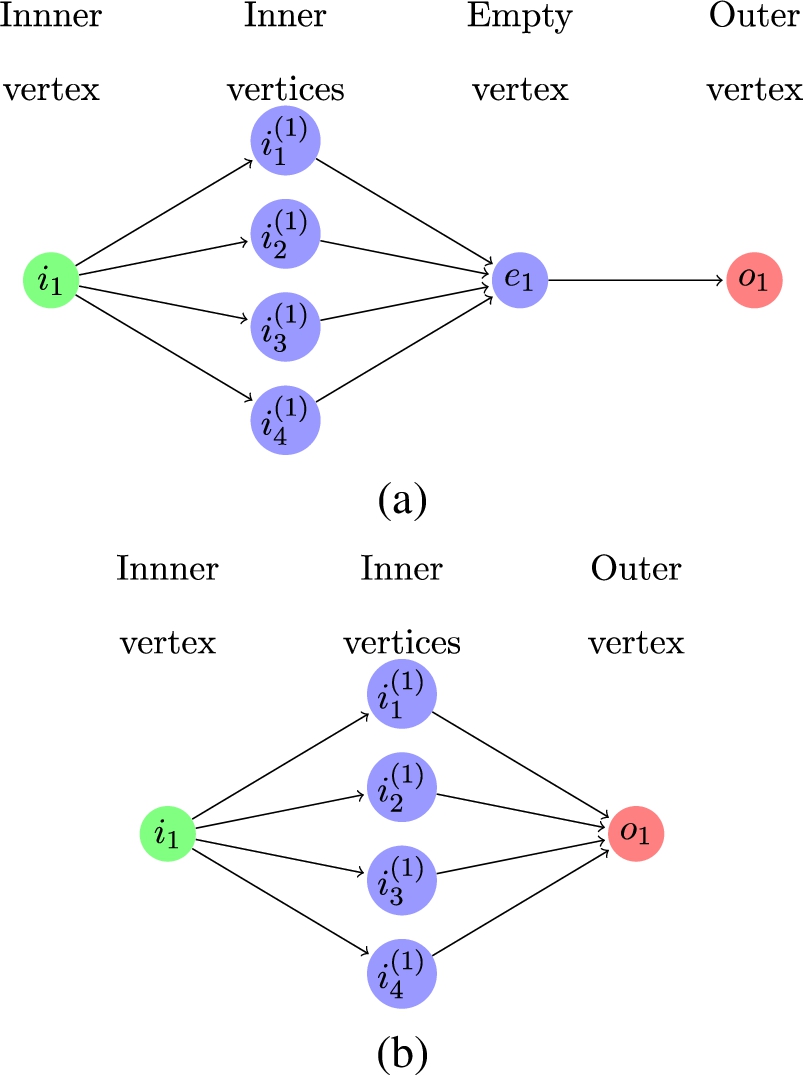
The graphical interpretation of Theorem 3.10, is that each empty vertex together with the edges connected to it is replaced by one edge ! (see Fig. 2(b)).

We denote the collections of connected Feynman graphs of n-th order by $G_{c} (n)$ . We construct this collections of graphs as follows:

For a given Feynman graph $G \in G (n)$ . Let $1 ⩽ q ⩽ n$ , we say that the graph connects q and j in notation $q \sim_{R} j$ , if the inner vertices $i_{q}$ and $i_{j}$ are connected in G. Clearly $\sim_{R}$ is an equivalence relation and if $I = {I_{1}, \dots, I_{k}}$ is the equivalence classes of $\sim_{R}$ then $I \in P ({1 \dots 2 n})$ . For $1 ⩽ l ⩽ k$ we denote by $G_{l} \in G_{c} (l)$ the connected Feynman graph with $n_{l}$ inner vertices such that $n = n_{1} + n_{2} + \dots + n_{k}$ , and we assign an analytic value to each connected graph $G_{l}$ denoted by $Υ_{c} (G) (t, x) : = Υ_{c} (G)$ .
Definition 3.12.
Let $G \in G_{c} (l)$ and $S \subset {1, \dots, 2 n_{l}}$ , we define the number $Υ_{c} (G)$ as follows:
For each inner vertex $i_{m}$ , $m \in {1, \dots n}$ , assign an index $j_{m} \in {1 \dots d}$ to each edge connected to $i_{m}$ .

For $l \in {1, \dots, 2 n}$ , multiply by $q_{t} (x) \int_{B} v_{t_{l}} d t_{l}$ , $B \in B (R^{d})$ each outer vertex connected to the l-th edge.

For m distinct ways of connecting edges to vertices that yields the same diagram, i.e., same topology, multiply by the combinatoric factor ${(- 2)}^{m} c_{m}$ , where $m = ♯ S$ and $c_{m}$ are the coefficients given by Theorem 3.10.

Sum up over $j_{1} \dots j_{2 n}$ .

We have established the following result:
Theorem 3.13.
The transition probability density $p_{t}$ , $t > 0$ of the semigroup ${(P_{t})}_{t ⩾ 0}$ associated to the solution $u_{t}$ , $t ⩾ 0$ of the stochastic differential equation (1) is expressed in terms of connected Feynman graphs $G \in G_{c} (n)$ whose analytic values $Υ_{c} (G) (t, x)$ , are fixed in Definition 3.12 i.e. $\begin{matrix} (28) & p_{t} (x) = \sum_{n = 0}^{\infty} {(- β)}^{n} \sum_{G \in G_{c} (n)} Υ_{c} (G) (t, x) . \end{matrix}$

Figures 2(a) and (b) give a construction of a connected Feynman graph and a graphical interpretation of Theorem 3.10.

Fig. 2.
(a) Example of a Feynman graph with 5 inner vertices, one empty vertex and one outer vertex. (b) Construction of a connected Feynman graph (from the graph in figure (a)) where the empty vertex together with the edges connected to it is replaced by one edge.
4. Asymptotic expansion of the transition probability density

The expansion of the transition probability density $p_{t}$ , $t > 0$ of the semigroup ${(P_{t})}_{t ⩾ 0}$ associated to the solution $u_{t}$ , $t ⩾ 0$ of the stochastic differential equation (1) given by Theorem 3.13 is divergent in general since the corresponding terms are rapidly unwieldy, however it can be given the meaning of an asymptotic expansion in the sense of Borel, see, e.g., [40]. In this section we recall the main result of this paper which proves the asymptotic behaviour of the transition probability density $p_{t}^{β} : = p_{t}$ , $t > 0$ as $β ⟶ \infty$ .

Definition 4.1.
For f, g two functions defined on $R$ , we have: $f (t) = O (g (t))$ , as $t \to + \infty$ , if $\exists L > 0$ , such that $| f (t) | ⩽ L | g (t) |$ .

The following result, due to George Neville Watson (1886–1965) is one of the significant result in the theory of asymptotic expansion:
Theorem 4.2 (Watson’s Lemma).

Suppose $f (t) = O (e^{m t})$ , $m \in R$ as $t \to + \infty$ and in some neighbourhood of $t = 0$ , $f (t)$ can be expanded as $\begin{matrix} (29) & f (t) = \sum_{k = 0}^{n} m_{k} t^{α + k} + R_{n + 1} (t), 0 < t < ζ, α > - 1 \end{matrix}$ where $m_{k} \in R$ , $| R_{n + 1} (t) | < A t^{n + 1}$ for $0 < t < ζ$ and $A > 0$ . Then $\begin{matrix} (30) & F (s) = \int_{0}^{+ \infty} e^{- s t} f (t) d t \end{matrix}$ has the asymptotic expansion $\begin{matrix} (31) & F (s) \sim \sum_{k = 0}^{\infty} m_{k} \frac{Γ (α + k + 1)}{s^{α + k + 1}}, s \to + \infty, \end{matrix}$

where Γ is the gamma function given by $Γ (t) = \int_{0}^{\infty} x^{t - 1} e^{- x} d x$ .

Definition 4.3.
Let $φ (γ)$ , $γ > 0$ be a given function. The series $\sum_{n = 0}^{\infty} φ_{n} γ^{n}$ is said to be asymptotic to $φ (γ)$ , if $\begin{matrix} (32) & \forall N \in N, φ (γ) - \sum_{n = 0}^{N} φ_{n} γ^{n} = O (γ^{N + 1}), as γ \to 0, \end{matrix}$ i.e., $\begin{matrix} (33) & | φ (γ) - \sum_{n = 0}^{N} φ_{n} γ^{n} | ⩽ C_{N + 1} γ^{N + 1}, for N \in N and C_{N + 1} > 0 . \end{matrix}$
Lemma 4.4.
Under the assumption given by equation (16) and for $g (t) = t^{\frac{1}{a}} \land t^{\frac{1}{b}}$ , there exists $K > 0$ such that: $\begin{matrix} (34) & q_{t} (x) ⩽ K {(g (t))}^{- d} . \end{matrix}$
Proof.
The proof can be found in [41], however we will develop other techniques by means of Fourier transform:

Since $q_{t}$ , $t > 0$ is characterized by the Fourier transform, see, equation (15), and from assumption (16), the following holds: $\begin{array}{rcl} q_{t} (x) & ⩽ & {(2 π)}^{- d} | \int_{R^{d}} e^{- x \cdot ξ} e^{- t Ψ (ξ)} d ξ | \\ ⩽ & {(2 π)}^{- d} \int_{R^{d}} | e^{- t Ψ (ξ)} | d ξ \\ = & {(2 π)}^{- d} \int_{R^{d}} e^{- t Re Ψ (ξ)} d ξ \\ ⩽ & {(2 π)}^{- d} (\int_{| ξ | ⩽ 1} e^{- c t | ξ |^{b}} d ξ + \int_{| ξ | ⩾ 1} e^{- c t | ξ |^{a}} d ξ) \\ = & {(2 π)}^{- d} (t^{- \frac{d}{b}} \int_{| ς | ⩽ t^{\frac{1}{b}}} e^{- c | ς |^{b}} d ς + t^{- \frac{d}{a}} \int_{| ς | ⩾ t^{\frac{1}{a}}} e^{- c | ς |^{a}} d ς) \\ (35) & = & c (t^{- \frac{d}{b}} + t^{- \frac{d}{a}}), \end{array}$ the result is immediate by taking $K = 2 c$ , ( $c > 0$ is given by equation (16)). □
Theorem 4.5.
The transition probability density $p_{t}$ , $t > 0$ given by Theorem 3.13 has an asymptotic expansion in power of β.
Proof.
From Theorem 3.13 we have $p_{t} (x) = \sum_{n = 0}^{\infty} {(- β)}^{n} \sum_{G \in G_{c} (n)} Υ_{c} (G) (t, x)$ , $β > 0$ ,it suffices then to prove: $\begin{matrix} (36) & | p_{t} - \sum_{n = 0}^{N} {(- β)}^{n} \sum_{G \in G_{c} (n)} Υ_{c} (G) (t, x) | ⩽ C_{N + 1} β^{N + 1}, for some constant C_{N} > 0 . \end{matrix}$ But $\begin{array}{rcl} | p_{t} - \sum_{n = 0}^{N} {(- β)}^{n} \sum_{G \in G_{c} (n)} Υ_{c} (G) (t, x) | & = & | \sum_{n = N + 1}^{\infty} {(- 1)}^{n} \sum_{G \in G_{c} (n)} Υ_{c} (G) (t, x) β^{n} | \\ ⩽ & K d^{2 N} ♯ P (1, \dots, 2 N) max_{I \in P (1, \dots, 2 N)} | \prod_{k = 0}^{n} Υ_{c} (G_{k}) | β^{N + 1}, \end{array}$ where in the last inequality we used the result given by Lemma 4.4, the factor $\prod_{k = 0}^{n} Υ_{c} (G_{k})$ is a real number associated with the graphs $G_{k}$ , $k = 0, \dots, n$ , $P (1, \dots, 2 N)$ is a partition of ${1, \dots, 2 N}$ , and $♯ P (1, \dots, 2 N)$ is the cardinal of $P (1, \dots, 2 N)$ .

Now if $B_{2 N} = ♯ P (1, \dots, 2 N)$ , then $B_{2 N}$ is nothing else then the “Bell numbers”, which counts in this case, the number of partitions of a set of size $2 N$ .

In the other hand from a result in [17], the authors proved that $\begin{matrix} (37) & \frac{ln N}{N} \sim ln N - ln (ln N) - 1 + \frac{ln (ln N) + 1}{ln N} + \frac{1}{2} {(\frac{ln (ln N)}{ln N})}^{2} . \end{matrix}$ From another result in [28], it has been shown that the Bell numbers $B_{N}$ are asymptotic to: $\begin{matrix} (38) & B_{N} \sim N^{- 1 / 2} ς {(N)}^{N + 1} e^{ς (N) - N - 1}, \end{matrix}$ with $ς (N)$ defined by $\begin{matrix} (39) & ς (N) = \frac{N}{W (N)}, \end{matrix}$ where $W (N)$ is the Lambert W-function, see, e.g. [23]. $ς (N)$ is also defined implicitly by $\begin{matrix} (40) & ς (N) ln ς (N) = N . \end{matrix}$ Putting together equation (37) and the properties of $W (N)$ , we have $ς (n) < n$ , therefore $\begin{matrix} (41) & \frac{B_{2 N}}{(2 N)!} ⩽ \frac{1}{\sqrt{2 π}} {(2)}^{2 N} e^{4 N} . \end{matrix}$ Hence $\begin{array}{rcl} | p_{t} - \sum_{n = 0}^{N} {(- β)}^{n} \sum_{G \in G_{c} (n)} Υ_{c} (G) (t, x) | & ⩽ & K d^{2 N} B_{2 N} max_{I \in P (1, \dots, 2 N)} | \prod_{k = 0}^{n} Υ_{c} (G_{k}) | β^{N + 1} \\ ⩽ & K d^{2 N} (2 N)! \frac{1}{\sqrt{2 π}} {(2)}^{2 N} e^{4 N} max_{I \in P (1, \dots, 2 N)} | \prod_{k = 0}^{n} Υ_{c} (G_{k}) | β^{N + 1} \\ (42) & ⩽ & C^{N + 1} β^{N + 1} . \end{array}$ Where in the last inequality C is a positive constant and we used Stirling’s formula, see, e.g., [29]. □
Proposition 4.6.
The integral $F (γ) = \int_{0}^{\infty} e^{- γ β} p_{t} d β$ has the asymptotic expansion: $\begin{matrix} (43) & F (γ) \sim \sum_{n = 0}^{\infty} {(- β)}^{n} \sum_{G \in G_{c} (n)} Υ_{c} (G) (t, x) \frac{n!}{γ^{n + 1}}, γ \to + \infty . \end{matrix}$
Proof.
By Theorem 4.5, the transition probability density $p_{t}$ , $t > 0$ has an asymptotic expansion in power of β, moreover it is expanded as: $\begin{matrix} (44) & p_{t} (x) = \sum_{n = 0}^{N} {(- 1)}^{n} \sum_{G \in G_{c} (n)} Υ_{c} (G) (t, x) β^{n} + R_{N + 1} (β), 0 < β < ζ, \end{matrix}$ where $R_{N + 1} (β) = \sum_{n = N + 1}^{\infty} {(- 1)}^{n} \sum_{G \in G_{c} (n)} Υ_{c} (G) (t, x) β^{n}$ and $| R_{N + 1} (t) | < \tilde{C} β^{N + 1}$ for $\tilde{C} > 0$ . Hence by Watson’s lemma, see, Theorem 4.2, we get: $\begin{matrix} (45) & F (γ) \sim \sum_{n = 0}^{\infty} {(- β)}^{n} \sum_{G \in G_{c} (n)} Υ_{c} (G) (t, x) \frac{Γ (n + 1)}{γ^{n + 1}}, γ \to + \infty . \end{matrix}$ The result is then immediate. □

5. Applications to stochastic and probabilistic neural networks

Artificial neural network (ANN) is an information processing that is inspired by the biological nervous system such as brain process information. In this section we will focus on two types of (ANN), namely stochastic and probabilistic neural networks.

5.1. Stochastic neural networks (SNN)

For SNN, the neurons will be modified either by stochastic transfer functions or given them stochastic weight.

To analyse the behaviour of models describing a network of interacting neurons, we apply our graph formalism, the graphs consists of m vertices (inner/outer and empty) and n edges where every vertex will be identified as a soma (body of the neuron cell) and every edge will represent a cylindrical which models the interaction between different neurons.

More precisely, we are concerned with a finite connected network, represented by a finite graph G with m edges $e_{1}, \dots, e_{m}$ and n vertices $v_{1}, \dots, v_{n}$ . Following, e.g. [31], we normalize and parametrize the edges to be identified with the interval $[0, 1]$ and we denote again by $e_{j} (\cdot)$ the parametrization of the edge $e_{j}$ (for more details about the above notation we refer to Mugnolo and all., see, e.g. [31,32]).

The valency of each vertex is denoted by $Γ (v_{i})$ ; precisely: $\begin{matrix} (46) & Γ (v_{i}) : = ♯ {j \in {1, \dots, m} : e_{j} (0) = v_{i} or e_{j} (1) = v_{i}}, 1 ⩽ i ⩽ n - 1 . \end{matrix}$ The graph G will be described then by the incidence matrix $Φ = Φ^{+} - Φ^{-}$ , where $Φ^{+} : = {(ϕ_{i j}^{+})}_{n \times m}$ and $Φ^{-} : = {(ϕ_{i j}^{-})}_{n \times m}$ are given by $\begin{matrix} ϕ_{i j}^{+} : = \{\begin{matrix} 1, & if e_{j} (0) = v_{i}; \\ 0, & otherwise, \end{matrix} and ϕ_{i j}^{-} : = \{\begin{matrix} 1, & if e_{j} (1) = v_{i}; \\ 0, & otherwise . \end{matrix} \end{matrix}$

For functions $u : G \to R$ , with an abuse of notation, we use the abbreviations $u_{j} (t, v_{i}) : = u_{j} (v_{i})$ to denote their values at 0 or 1, if $e_{j} (0) = v_{i}$ or $e_{j} (1) = v_{i}$ , respectively.

On G we consider the following system of stochastic diffusion equations: $\begin{matrix} (47) & \{\begin{matrix} \partial_{t} u_{j} (t, x) = \partial_{x} (c_{j} (x) \partial_{x} u_{j} (x)) + p_{j} (x) u_{j} (x) + f_{j} (u_{j} (t, x)) + β_{j} (t) \\ x \in (0, 1), t > 0, j = 1, \dots, m . \end{matrix} \end{matrix}$

In the above equations, $c_{j}$ and $p_{j}$ ( $j = 1, \dots, m$ ) are suitable smooth functions, while $f_{j}$ , $j = 1, \dots, m$ are suitable polynomials with odd degree. Moreover, ${(β_{j} (t))}_{t ⩾ 0}$ , $j = 1, \dots, m$ represents the stochastic perturbation acting on each edges due to external surrounding, and $β_{j} (t)$ is the distributional derivative of the process $β_{j}$ . Biological motivations lead to model this term by a Gaussian process. In fact, the evolution of the electrical potential on the molecular level can be perturbed by different types of random terms, each modeling the influence, at different time scales,of the surrounding medium. The generality of the above diffusion is motivated by the discussion in the biological literature.

The above equations shall be endowed with suitable boundary and initial conditions. Since we are dealing with a diffusion in a network, we require, following for example [31,32], a continuity assumption and a Kirchhoff’s law on every nodes: $\begin{matrix} (48) & \{\begin{matrix} u_{j} (v_{i}) = u_{k} (v_{i}), j, k \in Γ (v_{i}), i = 1, \dots, n \\ \sum_{j = 1}^{m} ϕ_{i j} μ_{j} c_{j} (v_{i}) \partial_{x} u_{j} (v_{i}) = 0, i = 1, \dots, n, μ_{j} > 0 . \end{matrix} \end{matrix}$ Initial conditions at time $t = 0$ are taken for simplicity to be of the form $\begin{matrix} (49) & u_{j} (0, x) = u_{j}^{0} (x) \in C ([0, 1]), j = 1, \dots, m . \end{matrix}$ Applying now the results recalled in Section 3, we can find the correlation functions $⟨ β_{j} (t_{1}) \dots β_{j} (t_{n}) ⟩$ which plays a central role in the Gaussian or Lévy process picture of wide networks (see, e.g. [11,42]). For instance if $β_{j}$ , $j = 1, \dots, m$ is Gaussian process centered at $t_{1}$ , $t_{2}$ , $t_{3}$ , $t_{4}$ „ the correlation function of linear networks are expressed in terms of covariances: $\begin{array}{rcl} ⟨ β_{j} (t_{1}) β_{j} (t_{2}) β_{j} (t_{3}) β_{j} (t_{4}) ⟩ & = & ⟨ β_{j} (t_{1}) β_{j} (t_{2}) ⟩ ⟨ β_{j} (t_{3}) β_{j} (t_{4}) ⟩ + ⟨ β_{j} (t_{1}) β_{j} (t_{3}) ⟩ ⟨ β_{j} (t_{2}) β_{j} (t_{4}) ⟩ \\ (50) & + ⟨ β_{j} (t_{1}) β_{j} (t_{4}) ⟩ ⟨ β_{j} (t_{2}) β_{j} (t_{3}) ⟩, j = 1, \dots, m . \end{array}$ As an example, for a linear networks with 2 hidden layers, and following Proposition 3.5 and Theorem 3.10 we will have: $\begin{matrix} (51) & ⟨ u_{j} (t, x_{1}) u_{j} (t, x_{2}) ⟩ = γ x_{1} x_{2} \sum_{i, j, k, l = 1}^{d} δ_{i k} δ_{i k} δ_{j i} δ_{i j} = x_{1}^{T} x_{2}, γ \in R, j = 1, \dots, m . \end{matrix}$ Where the last equality holds by taking $γ = \frac{1}{d^{2}}$ . Here $δ_{n n^{'}}$ being the Kronecker delta functions.

For multilayer network, if $p_{t} (x)$ , $t > 0$ is the probability density, where x is the network input, the out put will be then the estimate of $p_{t} (x)$ .

For $j = 1, \dots, m$ and from the results given in Section 3, the probability density $p_{t}$ , $t > 0$ will be given by the following expansion: $\begin{matrix} (52) & \begin{matrix} p_{t} (x) & = q_{t} (x) \sum_{i = 0}^{\infty} {(- β)}^{i} \\ \times E [\int_{0}^{t} u_{j} (x, τ_{1}) \int_{0}^{τ_{1}} u_{j} (x, τ_{2}) \dots \int_{0}^{τ_{i - 1}} u_{j} (x, τ_{i}) d τ_{1} \dots d τ_{i}], β > 0 . \end{matrix} \end{matrix}$ Since the estimation of the probability density is done in discrete case (through estimation of graphs), the neural networks methods will be more realistic.

From the above example we notice that correlation functions of linear network are simplified and consequently the expansion of the transition probability density $p_{t}$ , $t > 0$ can be approximated through the new simplified Feynman graphs and rules as follows:

Definition 5.1.
For a correlation function $C (u_{1}, \dots, u_{m})$ of a network with d hidden layers. We define the set of all Feynman graph $G$ as follows:
For each inner vertex $m \in {1, \dots, n}$ assign an index $j_{m} \in {1, \dots, d}$ corresponding to each edge connected to it.

Multiply with $X^{T} X$ each empty vertex connected to the m-th edge, where $X^{T} X = C (u_{1}, \dots, u_{m})$ .

5.2. Probabilistic neural networks (PNN)

For the case of (PNN), the probability distribution of each class is approximated by a distribution. Our current work can be also applied, since from Definitions 2.1, 3.7 and Remark 2.3, a Markov process $u_{t}$ , $t ⩾ 0$ can be given as a graph $G (V, E, p_{t})$ , where V (resp. E) is the set of vertices (resp. edges) and $p_{t}$ , $t > 0$ the transition probabilities along the edges between the vertices. (See Theorem 3.13 for the expression of $p_{t}$ .) Therefore the PNN can be defined as follows:

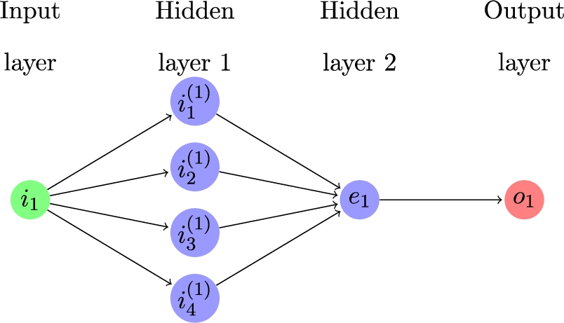
Given an input values (vectors product and bias value), which passes through a linear function to produce output values, in our approach, the input can be connected to several vertices (neurons) yields a hidden layer, the later can be also connected to other layers to produce out put layer all together leads a PNN. (See Fig. 3.)

Fig. 3.

Example of probabilistic neural network.

If an input layer $i_{k}$ is connected to hidden layers and leads an output $o_{1}$ , the transition probabilities $p_{t} (o_{1} | U = i_{k})$ can be approximated, as done in this work, and consequently one can generate arbitrary number of input/output, see, e.g. [42]. A simple example arise when we consider the Gaussian case, the transition probabilities densities are given by: $\begin{matrix} (53) & p_{t} (o_{1}) = \frac{1}{\sqrt{2 π} σ^{2}} e^{- \frac{∥ o_{1} - i_{k} - e_{1} ∥}{2 σ^{2}}}, k = 1, \dots, 4 . 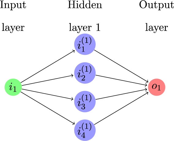\end{matrix}$ Now application of Theorem 3.13, the graphical representation of the probabilistic neural network given by Fig. 3 becomes as in Fig. 4, and the transition probabilities densities will be then given by: $\begin{matrix} (54) & p_{t} (o_{1}) = \frac{1}{\sqrt{2 π} σ^{2}} e^{- \frac{∥ o_{1} - i_{k} ∥}{2 σ^{2}}}, k = 1, \dots, 4 . \end{matrix}$

Fig. 4.

Example of PNN where the hidden layer 1 is connected directly to the output layer.

Footnotes

Acknowledgements

This work was supported by King Fahd University of Petroleum and Minerals under the project ♯ SB181034. The author gratefully acknowledges this support.

The author would like to thank Sergio Albeverio for many stimulating discussions.

References

Albeverio,

Dipersio,

Mastrogiacomo and

Smii, A class of Lévy driven SDEs and their explicit invariant measures, Pot. Anal. 45(2) (2016), 229–259. doi:10.1007/s11118-016-9544-3.

Albeverio ,

Dipersio,

Mastrogiacomo and

Smii, Explicit invariant measures for infinite dimensional SDE driven by Lévy noise with dissipative nonlinear drift I, Comm. Math. Sci. 15(4) (2017), 957–983. doi:10.4310/CMS.2017.v15.n4.a3.

Albeverio,

Gottschalk and

J.-L.

Wu, Convoluted generalized white noise, Schwinger functions and their analytic continuation to Wightman functions, Rev. Math. Phys 8(6) (1996), 763–817. doi:10.1142/S0129055X96000287.

Albeverio,

Lytvynov and

Mahnig, A model of the term structure of interest rates based on Lévy fields, Stoch. Proc. Appl. 114(2) (2004), 251–263. doi:10.1016/j.spa.2004.06.006.

Albeverio,

Mandrekar and

Rüdiger, Existence of mild solutions for stochastic differential equations and semilinear equations with non-Gaussian Lévy noise, Stochastic Process. Appl. 119(3) (2009), 835–863. doi:10.1016/j.spa.2008.03.006.

Albeverio,

Mastrogiacomo and

Smii, Small noise asymptotic expansions for stochastic PDE’s driven by dissipative nonlinearity and Lévy noise, Stoch. Proc. Appl. 123 (2013), 2084–2109. doi:10.1016/j.spa.2013.01.013.

Albeverio and

Smii, Asymptotic expansions for SDE’s with small multiplicative noise, Stoch. Process. App. 125(3) (2015), 1009–1031. doi:10.1016/j.spa.2014.09.009.

Albeverio and

Smii, Borel summation of the small time expansion of some SDE’s driven by Gaussian white noise, Asymp. Anal. 114 (2019), 211–223. doi:10.3233/ASY-191525.

Albeverio,

J.-L.

Wu and

T.S.

Zhang, Parabolic SPDEs driven by Poisson white noise, Stoch. Proc. Appl. 74 (1998), 21–36. doi:10.1016/S0304-4149(97)00112-9.

10.

O.E.

Barndorff-Nielsen and

Shephard , Non-Gaussian Ornstein–Uhlenbeck-based models and some of their uses in financial economics, J. R. Stat. Soc. Ser. B Stat. Methodol. 63(2) (2001), 167–241. doi:10.1111/1467-9868.00282.

11.

Blake,

Kohli and

Rother, Markov Random Fields for Vision and Image Processing, The MIT Press, 2011.

12.

Boyarchenko,

Svetlana and

Sergi, Non-Gaussian Merton–Black–Scholes Theory, Vol. 9, World Scientific, Singapore, 2002.

13.

Brzeźniak and

Hausenblas, Uniqueness in law of the Itô integral with respect to Lévy noise, in: Seminar Stoch. Anal., Random Fields and Appl., Vol. VI, Birkhauser, Basel, 2011, pp. 37–57.

14.

K.L.

Chung and

Rao, General gauge theorem for multiplicative functional, Trans. Am. Math. Soc. 306 (1988), 819–836. doi:10.1090/S0002-9947-1988-0933320-1.

15.

Cont and

Tankov, Financial Modelling with Jump Processes, Vol. 2, CRC Press, 2004.

16.

Ph.

Courrège, Sur la forme intégro-différentielle des opérateurs de

C_{k}^{\infty} (R^{n})

dans

C (R^{n})

satisfaisant au principe du maximum”, Sém. Théorie du potentiel (1965/66) Exposé 2.

17.

N.G.

De Bruijn, Asymptotic Methods in Analysis, North-Holland, Amsterdam, 1958, Zbl. 82,42 (2nd ed. 1975, 3rd ed., New York: Dover 1981).

18.

Eberlein and

Glau, Variational solutions of the pricing PIDEs for European options in Lévy models, Appl. Math. Finance (2014).

19.

Freidlin, Markov Processes and Differential Equations, Asymptotic Problems, Birkhäuser, Basel, 1996.

20.

I.I.

Gihman and

A.V.

Skorohod, Stochastic Differential Equations, Springer-Verlag, Berlin–Heidelberg. New York, 1972.

21.

Gottschalk and

Smii, How to determine the law of the solution to a SPDE driven by a Lévy space–time noise, Journal of Mathematical Physics 43 (2007), 1–22.

22.

Gottschalk,

Smii and

Thaler, The Feynman graph representation of general convolution semigroups and its applications to Lévy statistics, Journal of Bernoulli Society 14(2) (2008), 322–351. doi:10.3150/07-BEJ106.

23.

R.L.

Graham ,

D.E.

Knth and

Patashnik , Concrete Mathematics, Addison-Wesley, 1994.

24.

Hartman and

Wintner, On the infinitisimal generators of integral convolutions, Am. J. Math. 64 (1942), 273–298. doi:10.2307/2371683.

25.

Knopova, On the Feynman–Kac semigroup for some Markov processes, Mod. Stoch: Theor. App. 2 (2015), 107–129. doi:10.15559/15-VMSTA26.

26.

Knopova and

R.L.

Schilling , A note on the existence of transition probability densities of Lévy processes, Foru. Math. 25 (2013), 125–149.

27.

Løkka,

Øksendal and

Proske, Stochastic partial differential equations driven by Lévy space–time white noise, Ann. Appl. Prob. 14 (2004), 1506–1528. doi:10.1214/105051604000000413.

28.

Lovász, Combinatorial Problems and Exercises, 2nd edn, North Holland, Amsterdam, Netherlands, 1993.

29.

Marsaglia and

J.C.W.

Marsaglia, A new derivation of Stirling’s approximation of

n!

, Amer. Math. Monthly 97 (1990), 826–829. doi:10.1080/00029890.1990.11995666.

30.

Meyer-Brandis and

Proske, Explicit representation of strong solutions of SDEs driven by infinite dimensional Lévy processes, J. Theor. Prob. 23 (2010), 301–314. doi:10.1007/s10959-009-0226-6.

31.

Mugnolo, Gaussian estimates for a heat equation on a network, Netw. Heter. Media 2 (2007), 55–79. doi:10.3934/nhm.2007.2.55.

32.

Mugnolo and

Romanelli, Dynamic and generalized Wentzell node conditions for network equations, Math. Meth. Appl. Sciences 30 (2007), 681–706. doi:10.1002/mma.805.

33.

Øksendal, Stochastic Differential Equations: An Introduction with Applications, 6th edn, Springer-Verlag, Berlin Heidelberg, 2010.

34.

K.I.

Sato, Lévy Processes and Infinite Divisibility, Cambridge University Press, 1999.

35.

L.S.

Schulman, Techniques and Applications of Path Integrations, John Wiley and Sons, New York, 1981.

36.

J.-P.

Serre, Trees, Springer, Berlin, 1980.

37.

Shiga, A recurrence criterion for Markov processes of Ornstein–Uhlenbeck type, Prob. Th. Rel. Fields. 85 (1990), 425–447. doi:10.1007/BF01203163.

38.

Smii, A linked cluster theorem of the solution of the generalized Burger equation, Applied Mathematical Sciences. (Ruse) 6(1) (2012), 21–38.

39.

Smii, A large diffusion expansion for the transition function of Lévy Ornstein–Uhlenbeck processes, Appl. Math. Inf. Sci. 10(4) (2016), 1–8. doi:10.18576/amis/100434.

40.

A.D.

Sokal, An improvement of Watson’s theorem on Borel summability, J. Math. Phys. 21(2) (1980), 261–263. doi:10.1063/1.524408.

41.

Song, Two-sided estimates on the density of the Feynman–Kac semigroups of stable-like processes, Elec. J. Prob. 11 (2006), 146–161. doi:10.1214/EJP.v11-308.

42.

Turchetti, Stochastic Models of Neural Networks, IOS Press, 2004.