Vanishing viscosity limit for Riemann solutions to a 2 × 2 hyperbolic system with linear damping

Abstract

In this paper, we propose a time-dependent viscous system and by using the vanishing viscosity method we show the existence of solutions for the Riemann problem to a particular $2 \times 2$ system of conservation laws with linear damping.

Keywords

Nonstrictly hyperbolic system linear damping Riemann problem time-dependent viscous system delta shock wave solution

1. Introduction

In this paper, we study the existence of solutions to the Riemann problem for the following hyperbolic system of conservation laws with linear damping $\begin{matrix} (1) & \{\begin{matrix} u_{t} + \frac{1}{k + 1} {(u^{k + 1})}_{x} = - α u, \\ v_{t} + {(v u^{k})}_{x} = 0, \end{matrix} \end{matrix}$ where $α > 0$ is a constant, k is an odd natural number and the sign of v is assumed to be unchanging. Thus for convenience, we assume $v ⩾ 0$ throughout this paper. The initial data is given by $\begin{matrix} (2) & (v (x, 0), u (x, 0)) = \{\begin{matrix} (v_{-}, u_{-}), & if x < 0, \\ (v_{+}, u_{+}), & if x > 0, \end{matrix} \end{matrix}$ for arbitrary constant states $(v_{\pm}, u_{\pm})$ with $v_{\pm} > 0$ . It is well known that the system (1) is not strictly hyperbolic with eigenvalue $λ = u^{k}$ and right eigenvector $r = (1, 0)$ . Moreover, $\nabla λ \cdot r = 0$ and therefore the system is linearly degenerate. When $k = 1$ , the homogeneous case of the system (1) is used to model the evolution of density inhomogeneities in matter in the universe [19, B. Late nonlinear stage, 3. Sticky dust]. The system (1) belongs to the class of triangular systems. The triangular systems of conservation laws arises in a wide variety of models in physics and engineering, see for example [10,17] and the references therein. For this reason, the triangular systems have been studied by many authors and several rigorous results have been obtained for this.

In 1993, Joseph [11] considered the Riemann problem for the homogeneous case of the system (1) with $k = 1$ . He used a parabolic regularization system to obtain an explicit formulae of the Riemann solutions. So, he constructed the weak limit of the approximation solution and this is defined as a delta shock wave type solution. Recently, De la cruz [5] solved the Riemann problem to the system (1) when $k = 1$ . His work include classical Riemann solution and delta shock wave solution.

In this paper, we are interested in finding solutions to the Riemann problem for the system (1) with inital data (2). Therefore, we propose the following time-dependent viscous system $\begin{matrix} (3) & \{\begin{matrix} u_{t} + \frac{1}{k + 1} {(u^{k + 1})}_{x} = ε \frac{1}{α k} e^{- α k t} (1 - e^{- α k t}) u_{x x} - α u, \\ v_{t} + {(v u^{k})}_{x} = 0, \end{matrix} \end{matrix}$ (where $α > 0$ is a constant) with initial data (2). In general, regularization methods are important because one can construct an approximate solution near the Riemann solution, opening the way to further works in areas such as numerical analysis, stability of solutions and many others. The viscous system (3) is well motivated by scalar conservation law with time-dependent viscosity $\begin{matrix} u_{t} + F {(u)}_{x} = G (t) u_{x x} . \end{matrix}$ where $G (t) > 0$ for $t > 0$ . When $F (u) = u^{2}$ the scalar equation is called the Burgers equation with time-dependent viscosity. The Burgers equation with time-dependent viscosity was studied as a mathematical model of the propagation of the finite-amplitude sound waves in variable-area ducts, where u is an acoustic variable, with the linear effects of changes in the duct area taken out, and the time-dependent viscosity $G (t)$ is the duct area [2,7,24]. The reader can find results concerning to the existence, uniqueness and explicit solutions to the Burgers equation with time-dependent viscosity with suitable conditions for $G (t)$ in [2,3,7,18,24,25,28,29] and references cited therein. The Burgers equation with time-dependent viscosity and linear damping was studied in [14] and their results include explicit solutions for differents $G (t)$ .

When $G (t) = ε t$ and $ε > 0$ , for systems of hyperbolic conservation laws with time-dependent viscosity we refered the works developed by Tupciev in [22] and Dafermos in [4]. The results obtained in [4] and [22] do not include delta shock waves solutions. For systems of hyperbolic conservation laws with delta shock solutions the reader may consult [6,8,21,26,27].

When $G (t)$ is nonlinear, for systems of balance laws we refer to the work [5].

Note that our proposal of the time-dependent viscous system (3) is a special case of the general systems of conservation laws with time-dependent viscous system. Observe that if $(\hat{v}, \hat{u})$ solves $\begin{matrix} (4) & \{\begin{matrix} {\hat{u}}_{t} + \frac{1}{k + 1} e^{- α k t} {({\hat{u}}^{k + 1})}_{x} = ε \frac{1}{α k} e^{- α k t} (1 - e^{- α k t}) {\hat{u}}_{x x}, \\ {\hat{v}}_{t} + e^{- α k t} {(\hat{v} {\hat{u}}^{k})}_{x} = 0, \end{matrix} \end{matrix}$ with initial condition $\begin{matrix} (5) & (\hat{v} (x, 0), \hat{u} (x, 0)) = \{\begin{matrix} (v_{-}, u_{-}), & if x < 0, \\ (v_{+}, u_{+}), & if x > 0, \end{matrix} \end{matrix}$ then $(v, u)$ defined by $(v, u) = (\hat{v}, \hat{u} e^{- α t})$ solves the problem (3)–(2). We denote $({\hat{v}}^{ε}, {\hat{u}}^{ε})$ as $(\hat{v}, \hat{u})$ when there is no confusion. In order to solve the problem (4)–(5), we introduce the similarity variable ξ and solutions to (4) should approach for large times a similarity solution $(\hat{v}, \hat{u})$ to (4) of the form $\hat{v} (x, t) = \hat{v} (ξ)$ , $\hat{u} (x, t) = \hat{u} (ξ)$ and $ξ = a (t) x$ for some suitable smooth function $a (t) ⩾ 0$ for $t > 0$ (more details on the similarity methods can be found in [1,9,13,15,16,20] and references therein). Therefore, we introduce the similarity variable $ξ = \frac{α k x}{1 - e^{- α k t}}$ and the system (4) can be written as follows $\begin{matrix} (6) & \{\begin{matrix} - ξ {\hat{u}}_{ξ} + \frac{1}{k + 1} {({\hat{u}}^{k + 1})}_{ξ} = ε {\hat{u}}_{ξ ξ}, \\ - ξ {\hat{v}}_{ξ} + {(\hat{v} {\hat{u}}^{k})}_{ξ} = 0, \end{matrix} \end{matrix}$ and the initial data (5) changes to the boundary condition $\begin{matrix} (7) & (\hat{v} (\pm \infty), \hat{u} (\pm \infty)) = (v_{\pm}, u_{\pm}) . \end{matrix}$ Note that when $α \to 0 +$ , the similarity variable ξ converges to $x / t$ which is well used in many methods to study the behavior and structure of solutions of nonlinear hyperbolic systems of conservation laws. Notice that when $ε \to 0 +$ , the system (4) becomes $\begin{matrix} (8) & \{\begin{matrix} {\hat{u}}_{t} + \frac{1}{k + 1} e^{- α k t} {({\hat{u}}^{k + 1})}_{x} = 0, \\ {\hat{v}}_{t} + e^{- α k t} {(\hat{v} {\hat{u}}^{k})}_{x} = 0 . \end{matrix} \end{matrix}$ Using the vanishing viscosity method, and following works by Tan, Zhang and Zheng [21] and Ercole [8] with some appropriate modifications, we show the existence of solutions for system (6) with boundary condition (7). After, we study the behavior of the solutions $({\hat{v}}^{ε}, {\hat{u}}^{ε})$ as $ε \to 0 +$ to obtain classical Riemann solution and delta shock wave solution for the system (8). Finally, as $(v (x, t), u (x, t)) = (\hat{v} (x, t), \hat{u} (x, t) e^{- α t})$ , the solutions of (8) are used to obtain solutions of the original system (1).

The outline of the remaining of the paper is as follows. In Section 2, we show the existence of solutions to the viscous system (6) with boundary condition (7). In Section 3, we study the behavior of the solutions $({\hat{v}}^{ε}, {\hat{u}}^{ε})$ as $ε \to 0 +$ and we solve the Riemann problem to the system (4) without viscosity. In Section 4, we show classical Riemann solution and delta shock solution for the nonhomogeneous system (1). Final remarks are given in Section 5.

2. Existence of solutions to the viscous system (6)–(7)

Considering the first equation in (6) with boundary conditions, we have $\begin{matrix} (9) & \{\begin{matrix} - ξ {\hat{u}}_{ξ} + \frac{1}{k + 1} {({\hat{u}}^{k + 1})}_{ξ} = ε {\hat{u}}_{ξ ξ}, \\ \hat{u} (\pm \infty) = u_{\pm} . \end{matrix} \end{matrix}$ Now, based on the ideas of Dafermos [4], we consider the following boundary value problem with parameters $μ \in [0, 1]$ and $R > 1$ , $\begin{matrix} (10) & \{\begin{matrix} - ξ {\hat{u}}_{ξ} + \frac{μ}{k + 1} {({\hat{u}}^{k + 1})}_{ξ} = ε {\hat{u}}_{ξ ξ}, \\ \hat{u} (\pm R) = μ u_{\pm} . \end{matrix} \end{matrix}$

Lemma 2.1.
Let $\hat{u} (ξ)$ be a solution of ( 10 ) on $[- R, R]$ for some $μ > 0$ . Suppose that $u_{-} \neq u_{+}$ . Then, $\hat{u}$ is a strictly monotonic function on $[- R, R]$ .
Proof.
Observe that from (10) we have that $\begin{matrix} (11) & {\hat{u}}^{'} (ξ) = {\hat{u}}^{'} (ζ) exp (\int_{ζ}^{ξ} \frac{μ {\hat{u}}^{k} (s) - s}{ε} d s) \end{matrix}$ for any $ζ \in [- R, R]$ . Suppose $ξ_{1} \in [- R, R]$ is a critical point of $\hat{u} (ξ)$ , which implies ${\hat{u}}^{'} (ξ_{1}) = 0$ . Then, from (11) we have that ${\hat{u}}^{'} (ξ) = 0$ for all $ξ \in [- R, R]$ , and therefore $\hat{u} (ξ)$ is constant on $[- R, R]$ . But, this contradicts the fact that $u_{-} \neq u_{+}$ . Thus, $\hat{u} (ξ)$ is monotone. The monotonicity of $\hat{u} (ξ)$ depends on the value of ${\hat{u}}^{'} (ξ_{0})$ . If $u_{-} > u_{+}$ , then $\hat{u} (ξ)$ is strictly decreasing on $[- R, R]$ . When $u_{-} < u_{+}$ , we have that $\hat{u} (ξ)$ is strictly increasing on $[- R, R]$ . □
Theorem 2.2.
Suppose that $u_{-} \neq u_{+}$ . For every $ε > 0$ , there exists a smooth and monotone solution (not necessarily unique) of ( 9 ).
Proof.
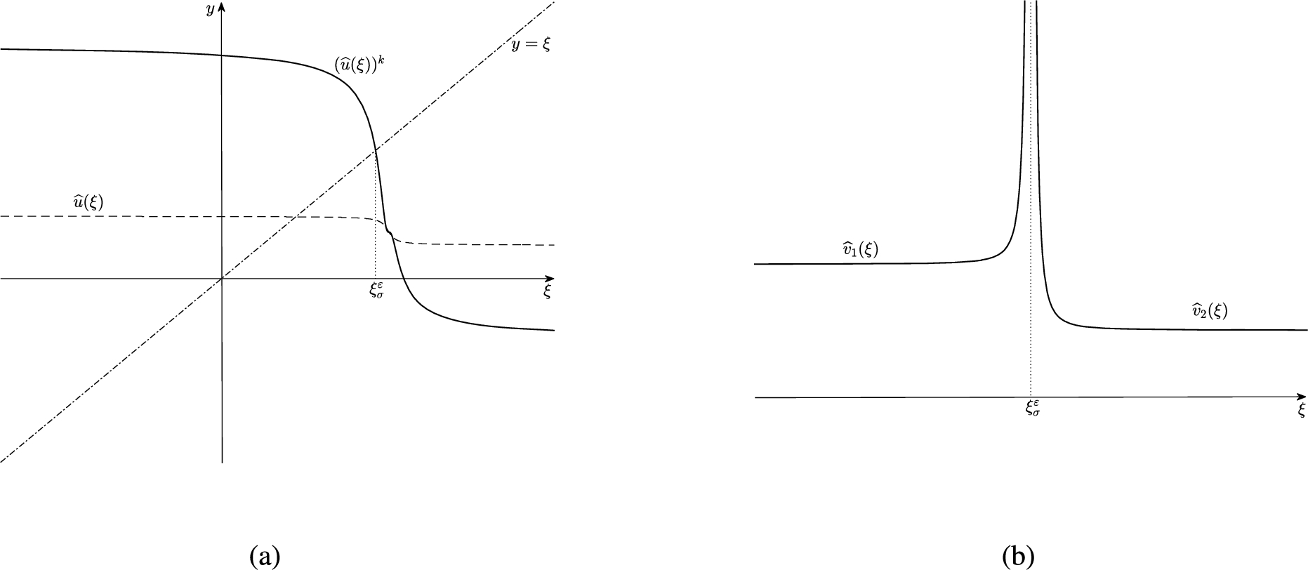
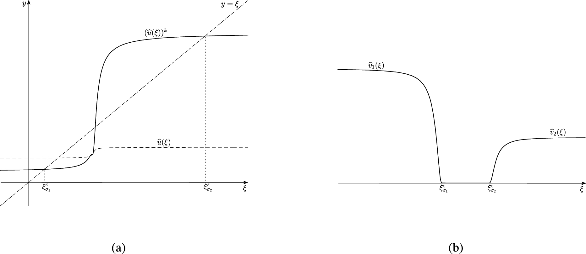
From Lemma 2.1, we have ${sup}_{- R < ξ < R} | \hat{u} (ξ) | ⩽ max {u_{-}, u_{+}}$ which does not depend on μ and R. Now, from Theorem 3.1 in [4] we conclude that there exists a solution of (9). Again combining the Lemma 2.1 and Theorem 3.1, we can take $R \to \infty$ and for the monotonicity of the solution in the previous lemma, we conclude that if $u_{-} > u_{+}$ , then the solution is decreasing on $(- \infty, \infty)$ , see Fig. 1(a). For $u_{-} < u_{+}$ , the solution is increasing on $(- \infty, \infty)$ , see Fig. 2(a). □

Fig. 1.
Graphs of the functions $\hat{u} (ξ)$ and $\hat{v} (ξ)$ in Theorem 2.2 and Lemma 2.5. (a-Left) For $u_{-} > u_{+}$ , the functions $\hat{u} (ξ)$ and ${(\hat{u} (ξ))}^{k}$ are monotonically decreasing. (b-Right) Graphs of the functions ${\hat{v}}_{1}$ and ${\hat{v}}_{2}$ .

Fig. 2.
Graphs of the functions $\hat{u} (ξ)$ and $\hat{v} (ξ)$ in Theorem 2.2 and Lemma 2.7. (a-Left) For $u_{-} < u_{+}$ , the functions $\hat{u} (ξ)$ and ${(\hat{u} (ξ))}^{k}$ are monotonically increasing. (b-Right) Graphs of the functions ${\hat{v}}_{1}$ and ${\hat{v}}_{2}$ .
Proposition 2.3.
Let $w (ξ)$ be a smooth solution of ( 9 ). Then, $\begin{matrix} | w^{'} (ξ) | ⩽ | w^{'} (0) | exp (\frac{2 u_{}^{k} | ξ | - ξ^{2}}{2 ε}), - \infty < ξ < + \infty, \end{matrix}$ where* $u_{} = max {u_{-}, u_{+}}$ .
Proof.
As w is a solution of (9), then $w (\pm \infty) = u_{\pm}$ . Now, multiplying the equation of (9) by $exp (\frac{ξ^{2}}{2 ε})$ , we have $\begin{matrix} \frac{d}{d ξ} (w^{'} (ξ) exp (\frac{ξ^{2}}{2 ε})) = \frac{1}{ε} w^{k} (ξ) w^{'} (ξ) exp (\frac{ξ^{2}}{2 ε}) \end{matrix}$ and integrating from 0 to ξ, we get, $\begin{matrix} (12) & w^{'} (ξ) exp (\frac{ξ^{2}}{2 ε}) = w^{'} (0) + \frac{1}{ε} \int_{0}^{ξ} w^{k} (s) w^{'} (s) exp (\frac{s^{2}}{2 ε}) d s . \end{matrix}$ From Theorem 2.2, we know that w is monotone and we have $| w (ξ) | ⩽ u_{}$ and $| w (ξ) |^{k} ⩽ u_{}^{k}$ for all ξ. Therefore, from (12) we obtain $\begin{array}{l} | w^{'} (ξ) exp (\frac{ξ^{2}}{2 ε}) | & ⩽ | w^{'} (0) | + \frac{1}{ε} \int_{0}^{ξ} | w^{k} (s) | | w^{'} (s) exp (\frac{s^{2}}{2 ε}) | d s \\ ⩽ | w^{'} (0) | + \frac{u_{}^{k}}{ε} \int_{0}^{ξ} | w^{'} (s) exp (\frac{s^{2}}{2 ε}) | d s \end{array}$ and using Gronwall’s inequality, we get the estimate $\begin{matrix} | w^{'} (ξ) | ⩽ | w^{'} (0) | exp (\frac{2 u_{}^{k} | ξ | - ξ^{2}}{2 ε}) . \end{matrix}$ □
Theorem 2.4.
Let* $u_{1} (ξ)$ and $u_{2} (ξ)$ be two smooth solutions of ( 9 ). Then, $u_{1} = u_{2}$ .
Proof.
Let ${\hat{u}}_{1} (ξ)$ and ${\hat{u}}_{2} (ξ)$ be solutions of the problem (9) and $\hat{U} (ξ) : = {\hat{u}}_{1} (ξ) - {\hat{u}}_{2} (ξ)$ . Then, from (9) we have that $\hat{U}$ is a smooth solution of the boundary value problem $\begin{matrix} (13) & \{\begin{matrix} - ξ {\hat{U}}_{ξ} + \frac{1}{k + 1} {(\hat{U} h)}_{ξ} = ε {\hat{U}}_{ξ ξ}, \\ \hat{U} (\pm \infty) = 0, \end{matrix} \end{matrix}$ where $h (ξ) = \int_{0}^{1} (k + 1) {({\hat{u}}_{1} (ξ) + ({\hat{u}}_{2} (ξ) - {\hat{u}}_{1} (ξ)) θ)}^{k} d θ$ . We note that $h (ξ)$ is bounded. Observe that from Proposition 2.3, we have $\begin{matrix} | {\hat{U}}^{'} (ξ) | ⩽ (| u_{1}^{'} (0) | + | u_{2}^{'} (0) |) exp (\frac{2 u_{}^{k} | ξ | - ξ^{2}}{2 ε}) \end{matrix}$ and ${\hat{U}}^{'} (ξ)$ decays rapidly to zero when $| ξ | \to \infty$ for each fixed $ε > 0$ . Therefore, when ${lim}_{ξ \to \pm \infty} \hat{U} (ξ) = 0$ we have ${lim}_{ξ \to \pm \infty} ξ \hat{U} (ξ) = 0$ .

Let us suppose that $\hat{U}$ is not the null function. Let a and b be consecutive zeros of $\hat{U}$ with $- \infty ⩽ a < b ⩽ + \infty$ . So, integrating (13) by parts on $(a, b)$ we find $\begin{matrix} (14) & ε ({\hat{U}}^{'} (b) - {\hat{U}}^{'} (a)) = \int_{a}^{b} \hat{U} (ξ) d ξ . \end{matrix}$ Now, if $\hat{U} > 0$ on $(a, b)$ , then ${\hat{U}}^{'} (b) ⩽ 0 ⩽ {\hat{U}}^{'} (a)$ and $\int_{a}^{b} \hat{U} (ξ) d ξ > 0$ . But, we have a contradiction with (14) because in this case (14) implies ${\hat{U}}^{'} (b) > {\hat{U}}^{'} (a)$ . In similar way, if $\hat{U} < 0$ on $(a, b)$ , then ${\hat{U}}^{'} (b) ⩾ 0 ⩾ {\hat{U}}^{'} (a)$ and $\int_{a}^{b} \hat{U} (ξ) d ξ > 0$ , which again contradicts with (14). Thus, we conclude that $\hat{U} \equiv 0$ . □

Putting $\hat{u} (ξ)$ into the second equation of (6) with boundary conditions (7), we get $\begin{matrix} (15) & \{\begin{matrix} - ξ {\hat{v}}_{ξ} + {(\hat{v} {\hat{u}}^{k})}_{ξ} = 0, \\ \hat{v} (\pm \infty) = v_{\pm} . \end{matrix} \end{matrix}$ The singularity point of (15) is given by the unique solution of ${(\hat{u} (ξ))}^{k} = ξ$ and it is denoted by $ξ_{σ}^{ε}$ . Observe that the solution of (15) can be obtained by pasting together the two solutions in the regions $(- \infty, ξ_{σ}^{ε})$ and $(ξ_{σ}^{ε}, + \infty)$ . Now integrating (15) from $- \infty$ to ξ for $ξ < ξ_{σ}^{ε}$ , we obtain $\begin{matrix} (16) & {\hat{v}}_{1} (ξ) = v_{-} exp (- \int_{- \infty}^{ξ} \frac{{({\hat{u}}^{k} (s))}^{'}}{{\hat{u}}^{k} (s) - s} d s) . \end{matrix}$ On the other hand, integrating (15) from ξ to $+ \infty$ for $ξ > ξ_{σ}^{ε}$ , we obtain $\begin{matrix} (17) & {\hat{v}}_{2} (ξ) = v_{+} exp (\int_{ξ}^{+ \infty} \frac{{({\hat{u}}^{k} (s))}^{'}}{{\hat{u}}^{k} (s) - s} d s) . \end{matrix}$
Lemma 2.5.
Suppose* $u_{-} > u_{+}$ . Let $\begin{matrix} (18) & \hat{v} (ξ) = \{\begin{matrix} {\hat{v}}_{1} (ξ), & if ξ < ξ_{σ}^{ε}, \\ {\hat{v}}_{2} (ξ), & if ξ > ξ_{σ}^{ε}, \end{matrix} \end{matrix}$ where $ξ_{σ}^{ε}$ is the unique solution of the equation ${(\hat{u} (ξ))}^{k} = ξ$ (which solution exists because $u_{-} > u_{+}$ and $\hat{u}$ is decreasing), ${\hat{v}}_{1}$ and ${\hat{v}}_{2}$ are defined by ( 16 ) and ( 17 ), respectively. Then $\hat{v} \in L^{1} (- \infty, + \infty)$ , $\hat{v}$ is continuous in $(- \infty, ξ_{σ}^{ε}) \cup (ξ_{σ}^{ε}, + \infty)$ and it is a weak solution for $\begin{matrix} (19) & - ξ {\hat{v}}_{ξ} + {(\hat{v} {\hat{u}}^{k})}_{ξ} = 0 . \end{matrix}$
Proof.
Note that from the formula (16), ${\hat{v}}_{1} (ξ)$ is monotonically increasing when $v_{-} > 0$ in the interval $(- \infty, ξ_{σ}^{ε})$ , and from (17) that ${\hat{v}}_{2} (ξ)$ is monotonically decreasing when $v_{+} > 0$ in the interval $(ξ_{σ}^{ε}, + \infty)$ (see Fig. 1(b)). Also, we have $\begin{matrix} lim_{ξ \to ξ_{σ}^{ε} -} {\hat{v}}_{1} (ξ) = + \infty, lim_{ξ \to ξ_{σ}^{ε} +} {\hat{v}}_{2} (ξ) = + \infty . \end{matrix}$

The equation (19) can be rewritten as $\begin{matrix} (20) & ({(\hat{u} (ξ))}^{k} - ξ) {\hat{v}}^{'} + \hat{v} {({(\hat{u} (ξ))}^{k})}^{'} = 0 . \end{matrix}$ Now, we can show that $\hat{v} \in L^{1} [ξ_{1}, ξ_{2}]$ for any interval $[ξ_{1}, ξ_{2}]$ containing $ξ_{σ}^{ε}$ . In fact, integrating (20) on $[ξ_{1}, ξ]$ for $ξ_{1} < ξ < ξ_{σ}^{ε}$ , we get $\begin{matrix} (21) & ({(\hat{u} (ξ))}^{k} - ξ) {\hat{v}}_{1} (ξ) - ({(\hat{u} (ξ_{1}))}^{k} - ξ_{1}) {\hat{v}}_{1} (ξ_{1}) + \int_{ξ_{1}}^{ξ} {\hat{v}}_{1} (s) d s = 0 . \end{matrix}$ Let $\begin{matrix} p (ξ) = \int_{ξ_{1}}^{ξ} {\hat{v}}_{1} (s) d s, A_{1} = ({(\hat{u} (ξ_{1}))}^{k} - ξ_{1}) {\hat{v}}_{1} (ξ_{1}) and a (ξ) = ({(\hat{u} (ξ))}^{k} - ξ) . \end{matrix}$ Then (21) can be written as $\begin{matrix} \{\begin{matrix} a (ξ) p^{'} (ξ) + p (ξ) = A_{1}, \\ p (ξ_{1}) = 0 . \end{matrix} \end{matrix}$ It follows that $\begin{matrix} p (ξ) = A_{1} {1 - exp (- \int_{ξ_{1}}^{ξ} \frac{d s}{a (s)})} . \end{matrix}$ Noting that $a (ξ) > 0$ and $a (ξ) = O (| ξ - ξ_{σ} |)$ as $ξ \to ξ_{σ}^{ε} -$ , we obtain $\begin{matrix} (22) & lim_{ξ \to ξ_{σ}^{ε} -} \int_{ξ_{1}}^{ξ} {\hat{v}}_{1} (s) d s = lim_{ξ \to ξ_{σ}^{ε} -} p (ξ) = A_{1} . \end{matrix}$ Hence $\begin{matrix} (23) & lim_{ξ \to ξ_{σ}^{ε} -} ({(\hat{u} (ξ))}^{k} - ξ) {\hat{v}}_{1} (ξ) = 0 . \end{matrix}$ Similarly, one can get $\begin{array}{l} (24) & \begin{aligned} lim_{ξ \to ξ_{σ}^{ε} +} \int_{ξ}^{ξ_{2}} {\hat{v}}_{2} (s) d s = A_{2}, \\ lim_{ξ \to ξ_{σ}^{ε} +} ({(\hat{u} (ξ))}^{k} - ξ) {\hat{v}}_{2} (ξ) = 0, \end{aligned} \end{array}$ where $A_{2} = ({(\hat{u} (ξ_{2}))}^{k} - ξ_{2}) {\hat{v}}_{2} (ξ_{2})$ . The equalities (22) and (24) imply that $\hat{v} (ξ) \in L^{1} ([ξ_{1}, ξ_{2}])$ .

Given an arbitrary function $ϕ \in C_{0}^{\infty} ([ξ_{1}, ξ_{2}])$ , we can show that $\begin{matrix} I \equiv - \int_{ξ_{1}}^{ξ_{2}} ({(\hat{u} (ξ))}^{k} - ξ) \hat{v} (ξ) ϕ^{'} (ξ) d ξ + \int_{ξ_{1}}^{ξ_{2}} \hat{v} (ξ) ϕ (ξ) d ξ = 0 . \end{matrix}$ Indeed, for any ${\tilde{ξ}}_{1}, {\tilde{ξ}}_{2}$ such that $ξ_{1} < {\tilde{ξ}}_{1} < ξ_{σ}^{ε} < ξ_{2} < R$ we can write $I = I_{1} + I_{2} + I_{3}$ , where $\begin{array}{l} I_{1} = \int_{ξ_{1}}^{\tilde{ξ_{1}}} (- ({(\hat{u} (ξ))}^{k} - ξ) \hat{v} (ξ) ϕ^{'} (ξ) + \hat{v} (ξ) ϕ (ξ)) d ξ, \\ I_{2} = \int_{\tilde{ξ_{1}}}^{\tilde{ξ_{2}}} (- ({(\hat{u} (ξ))}^{k} - ξ) \hat{v} (ξ) ϕ^{'} (ξ) + \hat{v} (ξ) ϕ (ξ)) d ξ and \\ I_{3} = \int_{\tilde{ξ_{2}}}^{ξ_{2}} (- ({(\hat{u} (ξ))}^{k} - ξ) \hat{v} (ξ) ϕ^{'} (ξ) + \hat{v} (ξ) ϕ (ξ)) d ξ . \end{array}$ Observe that $\begin{array}{l} | I_{1} | & = | - ({(\hat{u} (\tilde{ξ_{1}}))}^{k} - {\tilde{ξ}}_{1}) {\hat{v}}_{1} ({\tilde{ξ}}_{1}) ϕ ({\tilde{ξ}}_{1}) + \int_{ξ_{1}}^{\tilde{ξ_{1}}} ({(({(\hat{u} (ξ))}^{k} - ξ) \hat{v} (ξ))}^{'} ϕ (ξ) + \hat{v} (ξ) ϕ (ξ))) d ξ | \\ = | ({(\hat{u} ({\tilde{ξ}}_{1}))}^{k} - {\tilde{ξ}}_{1}) {\hat{v}}_{1} ({\tilde{ξ}}_{1}) ϕ ({\tilde{ξ}}_{1}) | . \end{array}$ By (23), we have that $\begin{matrix} lim_{{\tilde{ξ}}_{1} \to ξ_{σ}^{ε} -} | I_{1} | = lim_{{\tilde{ξ}}_{1} \to ξ_{σ}^{ε} -} | ({(\hat{u} ({\tilde{ξ}}_{1}))}^{k} - {\tilde{ξ}}_{1}) {\hat{v}}_{1} ({\tilde{ξ}}_{1}) ϕ ({\tilde{ξ}}_{1}) | = 0 . \end{matrix}$ In similar way, we show that $\begin{matrix} lim_{{\tilde{ξ}}_{2} \to ξ_{σ}^{ε} +} | I_{3} | = lim_{{\tilde{ξ}}_{2} \to ξ_{σ}^{ε} +} | ({(\hat{u} ({\tilde{ξ}}_{2}))}^{k} - {\tilde{ξ}}_{2}) {\hat{v}}_{2} ({\tilde{ξ}}_{2}) ϕ ({\tilde{ξ}}_{2}) | = 0 . \end{matrix}$ Since $\hat{v} \in L^{1} ([ξ_{1}, ξ_{2}])$ , $\begin{matrix} | I_{2} | ⩽ \int_{\tilde{ξ_{1}}}^{\tilde{ξ_{2}}} | - ({(\hat{u} (ξ))}^{k} - ξ) ϕ^{'} (ξ) + ϕ (ξ) | | \hat{v} (ξ) | d ξ \to 0, as {\tilde{ξ}}_{1} \to ξ_{σ}^{ε} -, {\tilde{ξ}}_{2} \to ξ_{σ}^{ε} + . \end{matrix}$ But I is independent of ${\tilde{ξ}}_{1}$ and ${\tilde{ξ}}_{2}$ , so $I = 0$ . Therefore, $\hat{v}$ defined in (18) is a weak solution. □
Remark 2.6.
Observe that in Lemma 2.5, the function ${\hat{v}}_{1} (ξ)$ is monotonically decreasing in the interval $(- \infty, ξ_{σ}^{ε})$ when $v_{-} < 0$ , while the function ${\hat{v}}_{2} (ξ)$ is monotonically increasing in the interval $(- \infty, ξ_{σ}^{ε})$ for $v_{+} < 0$ . Moreover, if $u_{-} > u_{+}$ , $v_{-} < 0$ and $v_{+} < 0$ , we have ${lim}_{ξ \to ξ_{σ}^{ε} -} {\hat{v}}_{1} (ξ) = - \infty$ and ${lim}_{ξ \to ξ_{σ}^{ε} +} {\hat{v}}_{2} (ξ) = - \infty$ .
Lemma 2.7.
Suppose $u_{-} < u_{+}$ . Let $\begin{matrix} \hat{v} (ξ) = \{\begin{matrix} {\hat{v}}_{1} (ξ), & if ξ < ξ_{σ_{1}}^{ε}, \\ 0, & if ξ_{σ_{1}}^{ε} ⩽ ξ ⩽ ξ_{σ_{2}}^{ε}, \\ {\hat{v}}_{2} (ξ), & if ξ > ξ_{σ_{2}}^{ε}, \end{matrix} \end{matrix}$ where ${\hat{v}}_{1}$ and ${\hat{v}}_{2}$ are defined by ( 16 ) and ( 17 ), respectively, $ξ_{σ_{1}}^{ε} ⩽ ξ_{σ_{2}}^{ε}$ satisfying $ξ_{σ_{1}}^{ε} = min {ξ : {(\hat{u} (ξ))}^{k} = ξ}$ , $ξ_{σ_{2}}^{ε} = max {ξ : {(\hat{u} (ξ))}^{k} = ξ}$ and ${lim}_{ξ \to ξ_{σ_{1}}^{ε} -} {\hat{v}}_{1} (ξ) = {lim}_{ξ \to ξ_{σ_{2}}^{ε} +} {\hat{v}}_{2} (ξ) = 0$ . Then $\hat{v} \in L^{1} (- \infty, + \infty)$ , ${\hat{v}}_{1}$ is decreasing in $(- \infty, ξ_{σ_{1}}^{ε})$ , ${\hat{v}}_{2}$ is increasing in $(ξ_{σ_{2}}^{ε}, + \infty)$ , $\hat{v}$ is continuous on the intervals $(- \infty, ξ_{σ_{1}}^{ε})$ and $(ξ_{σ_{2}}^{ε}, + \infty)$ , and it is a weak solution for $- ξ {\hat{v}}_{ξ} + {(\hat{v} {\hat{u}}^{k})}_{ξ} = 0$ .
Proof.
As $u_{-} < u_{+}$ , thus $\hat{u}$ is increasing. Consider now the function $s \mapsto s - {\hat{u}}^{k} (s)$ which is continuous and approaches $\pm \infty$ as $s \to \pm \infty$ . Hence, there exist finite quantities $ξ_{σ_{1}}^{ε} = min {ξ : {(\hat{u} (ξ))}^{k} = ξ}$ and $ξ_{σ_{2}}^{ε} = max {ξ : {(\hat{u} (ξ))}^{k} = ξ}$ . One has $s - {(\hat{u} (s))}^{k} < 0$ on $(- \infty, ξ_{σ_{1}}^{ε})$ and $s - {(\hat{u} (s))}^{k} > 0$ on $(ξ_{σ_{2}}^{ε}, + \infty)$ . Moreover, we can get $ξ_{σ_{1}}^{ε} ⩽ ξ_{σ_{2}}^{ε}$ . We now claim that $\begin{matrix} (25) & lim_{ξ \to ξ_{σ_{2}}^{ε} +} \int_{ξ}^{+ \infty} \frac{{({\hat{u}}^{k} (s))}^{'}}{s - {\hat{u}}^{k} (s)} d s = + \infty . \end{matrix}$ In fact, for R fixed and $ξ_{σ_{2}}^{ε} < ξ < R$ we have $\begin{array}{l} \int_{ξ}^{R} \frac{{({\hat{u}}^{k} (s))}^{'}}{s - {\hat{u}}^{k} (s)} d s & = {({\hat{u}}^{k} (ζ))}^{'} \int_{ξ}^{R} \frac{d s}{s - {\hat{u}}^{k} (s)} ⩾ {({\hat{u}}^{k} (ζ))}^{'} \int_{ξ}^{R} \frac{d s}{s - {\hat{u}}^{k} (ξ)} \\ = - {({\hat{u}}^{k} (ζ))}^{'} ln (\frac{ξ - {\hat{u}}^{k} (ξ)}{R - {\hat{u}}^{k} (ξ)}) \to + \infty, as ξ \to ξ_{σ_{2}}^{ε} +, \end{array}$ where $ξ ⩽ ζ ⩽ R$ . Now, from (17) and (25) we get $\begin{matrix} lim_{ξ \to ξ_{σ_{2}}^{ε} +} {\hat{v}}_{2} (ξ) = 0 . \end{matrix}$ In a similar way, we can obtain ${lim}_{ξ \to ξ_{σ_{1}}^{ε} -} {\hat{v}}_{1} (ξ) = 0$ . The monotonicity of ${\tilde{v}}_{1}$ and ${\hat{v}}_{2}$ is obvious, see Fig. 2(b). When $ξ_{σ_{1}}^{ε} ⩽ ξ ⩽ ξ_{σ_{2}}^{ε}$ , from (20) we have $\begin{matrix} \int_{ξ_{σ_{1}}^{ε}}^{ξ_{σ_{2}}^{ε}} ({(\hat{u} (ξ))}^{k} {\hat{v}}^{'} - ξ {\hat{v}}^{'} + \hat{v} {({(\hat{u} (ξ))}^{k})}^{'} d ξ = 0 \end{matrix}$ or $\begin{matrix} {(({(\hat{u} (ξ))}^{k} - ξ) \hat{v} (ξ) |}_{ξ_{σ_{1}}^{ε}}^{ξ_{σ_{2}}^{ε}} + \int_{ξ_{σ_{1}}^{ε}}^{ξ_{σ_{2}}^{ε}} \hat{v} (ξ) d ξ = 0 \end{matrix}$ which implies that $\hat{v} (ξ) = 0$ . □
3. The limit solutions of (4)–(5) as viscosity vanishes

In this section, we are interested in analyzing the behavior of the solutions $({\hat{v}}^{ε}, {\hat{u}}^{ε})$ of (6)–(7) as $ε \to 0 +$ to stablished the solutions of (4)–(5).

3.1. Case 1. $u_{-} > u_{+}$

Lemma 3.1.
Let $ξ_{σ}^{ε}$ be the unique point satisfying ${({\hat{u}}^{ε} (ξ_{σ}^{ε}))}^{k} = ξ_{σ}^{ε}$ , and let $ξ_{σ}$ be the limit $ξ_{σ} = {lim}_{ε \to 0 +} ξ_{σ}^{ε}$ (passing to a subsequence if necessary). Then for any $η > 0$ , $\begin{array}{l} lim_{ε \to 0 +} {\hat{u}}_{ξ}^{ε} (ξ) = 0, for | ξ - ξ_{σ} | ⩾ η, \\ lim_{ε \to 0 +} {\hat{u}}^{ε} (ξ) = \{\begin{matrix} u_{-}, & if ξ ⩽ ξ_{σ} - η, \\ u_{+}, & if ξ ⩾ ξ_{σ} + η, \end{matrix} \end{array}$ uniformly in the above intervals. Moreover, $ξ_{σ} = \frac{1}{k + 1} \sum_{j = 0}^{k} u_{-}^{k - j} u_{+}^{j}$ and $ξ_{σ} [u] - \frac{1}{k + 1} [u^{k + 1}] = 0$ .
Proof.
To simplify the notation in this proof, we shall use $\hat{v}$ , $\hat{u}$ instead of ${\hat{v}}^{ε}$ , ${\hat{u}}^{ε}$ .

Take $ξ_{3} = ξ_{σ} - η / 2$ , and let ε be so small such that $ξ_{σ}^{ε} > ξ_{3} + η / 4$ .

Now, integrating the first equation of (6) twice on $[ξ, ξ_{3}]$ , we get $\begin{array}{l} \hat{u} (ξ_{3}) - \hat{u} (ξ) & = {\hat{u}}^{'} (ξ_{3}) \int_{ξ}^{ξ_{3}} exp (- \int_{r}^{ξ_{3}} \frac{{(\hat{u} (s))}^{k} - s}{ε} d s) d r \\ ⩽ {\hat{u}}^{'} (ξ_{3}) \int_{ξ}^{ξ_{3}} exp (- \int_{r}^{ξ_{3}} \frac{u_{-}^{k} - s}{ε} d s) d r \\ = {\hat{u}}^{'} (ξ_{3}) \int_{ξ}^{ξ_{3}} exp (\frac{1}{ε} ((u_{-}^{k} - ξ_{3}) (r - ξ_{3}) - \frac{1}{2} {(r - ξ_{3})}^{2})) d r \\ = {\hat{u}}^{'} (ξ_{3}) \int_{ξ - ξ_{3}}^{0} exp (\frac{1}{ε} ((u_{-}^{k} - ξ_{3}) r - \frac{1}{2} r^{2})) d r . \end{array}$ Letting $ξ \to - \infty$ , we get $\begin{array}{l} u_{+} - u_{-} & ⩽ {\hat{u}}^{'} (ξ_{3}) \int_{- \infty}^{0} exp (\frac{1}{ε} ((u_{-}^{k} - ξ_{3}) r - \frac{1}{2} r^{2})) d r \\ ⩽ {\hat{u}}^{'} (ξ_{3}) \int_{0}^{2 ε} exp (- \frac{1}{ε} ((u_{-}^{k} - ξ_{3}) r + \frac{1}{2} r^{2})) d r \\ ⩽ {\hat{u}}^{'} (ξ_{3}) \sqrt{ε} A_{3} \end{array}$ for $0 ⩽ ε ⩽ 1$ , where $A_{3}$ is a constant independent of ε. Thus $\begin{matrix} | {\hat{u}}^{'} (ξ_{3}) | ⩽ \frac{u_{-} - u_{+}}{\sqrt{ε} A_{3}} . \end{matrix}$ So $\begin{matrix} (26) & | {\hat{u}}^{'} (ξ) | ⩽ \frac{u_{-} - u_{+}}{\sqrt{ε} A_{3}} exp (- \int_{ξ}^{ξ_{3}} \frac{{(\hat{u} (s))}^{k} - s}{ε} d s) . \end{matrix}$ Noticing that $\begin{array}{l} {(\hat{u} (s))}^{k} - s & = ({(\hat{u} (s))}^{k} - {(\hat{u} (ξ_{σ}^{ε}))}^{k}) - (s - ξ_{σ}^{ε}) = (k {(\hat{u} (θ))}^{k - 1} u^{'} (θ) - 1) (s - ξ_{σ}^{ε}) ⩾ \frac{η}{4} \end{array}$ for $s ⩽ ξ_{3}$ and from (26) we have $\begin{matrix} | {\hat{u}}^{'} (ξ) | ⩽ \frac{u_{-} - u_{+}}{\sqrt{ε} A_{3}} exp (- \frac{η}{4 ε} (ξ_{3} - ξ)) \end{matrix}$ which implies that $\begin{matrix} lim_{ε \to 0 +} {\hat{u}}_{ξ}^{ε} (ξ) = 0, uniformly for ξ ⩽ ξ_{σ} - η . \end{matrix}$ Now, we choose ξ and $ξ_{4}$ such that $ξ < ξ_{4} ⩽ ξ_{σ} - η$ . From $\begin{matrix} \hat{u} (ξ_{4}) - \hat{u} (ξ) = {\hat{u}}^{'} (ξ_{4}) \int_{ξ}^{ξ_{4}} exp (- \int_{r}^{ξ_{4}} \frac{{(\hat{u} (s))}^{k} - s}{ε} d s) d r, \end{matrix}$ we get $\begin{array}{l} | \hat{u} (ξ_{4}) - \hat{u} (ξ) | & ⩽ | {\hat{u}}^{'} (ξ_{4}) | \int_{ξ}^{ξ_{4}} exp (\frac{A_{4}}{ε} (r - ξ_{4})) d r ⩽ \frac{ε}{A_{4}} | {\hat{u}}^{'} (ξ_{4}) | (1 - exp (\frac{A_{4}}{ε} (ξ - ξ_{4}))), \end{array}$ where $A_{4} = {(\hat{u} (ξ_{4}))}^{k} - ξ_{4}$ . When $ξ \to - \infty$ , we obtain $\begin{matrix} | \hat{u} (ξ_{4}) - u_{-} | ⩽ \frac{ε}{A_{4}} | {\hat{u}}^{'} (ξ_{4}) |, \end{matrix}$ which implies that $\begin{matrix} lim_{ε \to 0 +} {\hat{u}}^{ε} (ξ) = u_{-}, uniformly for ξ ⩽ ξ_{σ} - η . \end{matrix}$ The results for $ξ ⩾ ξ_{σ} + η$ can be obtained analogously.

In fact, let $ϕ \in C_{0}^{\infty} ((ξ_{1}, ξ_{2}))$ where $ξ_{1} < ξ_{σ} < ξ_{2}$ , From (9) we have $\begin{matrix} (27) & \int_{ξ_{1}}^{ξ_{2}} \hat{u} (ξ) ({(ξ ϕ (ξ))}^{'} - \frac{1}{k + 1} {\hat{u}}^{k} (ξ) ϕ^{'} (ξ)) d ξ = ε \int_{ξ_{1}}^{ξ_{2}} \hat{u} (ξ) ϕ^{″} (ξ) d ξ . \end{matrix}$ Passing limit $ε \to 0 +$ in (27), we get $\begin{matrix} \int_{ξ_{1}}^{ξ_{σ}} u_{-} ({(ξ ϕ (ξ))}^{'} - \frac{1}{k + 1} u_{-}^{k} ϕ^{'} (ξ)) d ξ + \int_{ξ_{σ}}^{ξ_{2}} u_{+} ({(ξ ϕ (ξ))}^{'} - \frac{1}{k + 1} u_{+}^{k} ϕ^{'} (ξ)) d ξ = 0 . \end{matrix}$ or $\begin{matrix} u_{-} ξ_{σ} ϕ (ξ_{σ}) - \frac{1}{k + 1} u_{-}^{k + 1} ϕ (ξ_{σ}) - u_{+} ξ_{σ} ϕ (ξ_{σ}) + \frac{1}{k + 1} u_{+}^{k + 1} ϕ (ξ_{σ}) = 0 \end{matrix}$ which yields $ξ_{σ} = \frac{1}{k + 1} \sum_{j = 0}^{k} u_{-}^{k - j} u_{+}^{j}$ for arbitrary ϕ. □
Lemma 3.2.
For any $η > 0$ , $\begin{matrix} lim_{ε \to 0 +} {\hat{v}}^{ε} (ξ) = \{\begin{matrix} v_{-}, & if ξ < ξ_{σ} - η, \\ v_{+}, & if ξ > ξ_{σ} + η, \end{matrix} \end{matrix}$ uniformly, with respect to ξ.
Proof.
Take $ε_{0} > 0$ so small such that $| ξ_{σ}^{ε} - ξ_{σ} | < \frac{η}{2}$ whenever $0 < ε < ε_{0}$ . For any $ξ ⩾ ξ_{σ} + η$ and $ε < ε_{0}$ , we have $\begin{matrix} ξ > ξ_{σ}^{ε} + \frac{η}{2} \end{matrix}$ and $\begin{matrix} {\hat{v}}^{ε} (ξ) = v_{+} exp (\int_{ξ}^{\infty} \frac{{({({\hat{u}}^{ε} (s))}^{k})}^{'}}{{({\hat{u}}^{ε} (s))}^{k} - s} d s) . \end{matrix}$ For any $s \in [ξ, + \infty)$ , we have $\begin{array}{l} {({\hat{u}}^{ε} (s))}^{k} - s & < {({\hat{u}}^{ε} (ξ))}^{k} - ξ = (1 - {({({\hat{u}}^{ε} (ζ))}^{k})}^{'}) (ξ_{σ}^{ε} - ξ) ⩽ - \frac{η}{2} . \end{array}$ As $\hat{u}$ is decreasing, we have that ${({(\hat{u} (ξ))}^{k})}^{'} = k {(\hat{u} (ξ))}^{k - 1} {\hat{u}}^{'} (ξ) < 0$ , and $\begin{matrix} \frac{{({(\hat{u} (s))}^{k})}^{'}}{{({\hat{u}}^{ε} (s))}^{k} - s} < - \frac{2}{η} {({(\hat{u} (s))}^{k})}^{'}, for any s \in [ξ, + \infty) . \end{matrix}$ Now, in the last inequality, integrating on $[ξ, + \infty)$ we have $\begin{matrix} 0 ⩽ \int_{ξ}^{\infty} \frac{{({({\hat{u}}^{ε} (s))}^{k})}^{'}}{{({\hat{u}}^{ε} (s))}^{k} - s} d s ⩽ - \frac{2}{η} \int_{ξ}^{\infty} {({(u^{ε} (s))}^{k})}^{'} d s = - \frac{2}{η} (u_{+}^{k} - {({\hat{u}}^{ε} (ξ))}^{k}), \end{matrix}$ so $\begin{matrix} (28) & 1 ⩽ exp (\int_{ξ}^{\infty} \frac{{({({\hat{u}}^{ε} (s))}^{k})}^{'}}{{({\hat{u}}^{ε} (s))}^{k} - s} d s) ⩽ exp (- \frac{2}{η} (u_{+}^{k} - {({\hat{u}}^{ε} (ξ))}^{k})) . \end{matrix}$ By Lemma 3.1 we have that ${lim}_{ε \to 0 +} {\hat{u}}^{ε} (ξ) = u_{+}$ , and from (28) we have $\begin{matrix} lim_{ε \to 0 +} exp (\int_{ξ}^{\infty} \frac{{({({\hat{u}}^{ε} (s))}^{k})}^{'}}{{({\hat{u}}^{ε} (s))}^{k} - s} d s) = 1 \end{matrix}$ and $\begin{matrix} lim_{ε \to 0 +} {\hat{v}}^{ε} (ξ) = lim_{ε \to 0 +} v_{+} exp (\int_{ξ}^{\infty} \frac{{({({\hat{u}}^{ε} (s))}^{k})}^{'}}{{({\hat{u}}^{ε} (s))}^{k} - s} d s) = v_{+}, uniformly for ξ > ξ_{σ} + η . \end{matrix}$ Similarly, we obtain also ${lim}_{ε \to 0} {\hat{v}}^{ε} (ξ) = v_{-}$ , uniformly for $ξ < ξ_{σ} - η$ . □
Lemma 3.3.
Let $({\hat{u}}^{ε}, {\hat{v}}^{ε})$ be the solution of the Riemann problem ( 6 )–( 7 ) Denote $\begin{matrix} σ = ξ_{σ} = lim_{ε \to 0 +} ξ_{σ}^{ε} = lim_{ε \to 0 +} {({\hat{u}}^{ε} (ξ_{σ}^{ε}))}^{k} = {(\hat{u} (σ))}^{k} . \end{matrix}$ Then $\begin{matrix} lim_{ε \to 0 +} ({\hat{v}}^{ε} (ξ), {\hat{u}}^{ε} (ξ)) = \{\begin{matrix} (v_{-}, u_{-}), & if ξ < σ, \\ (w_{0} \cdot δ, σ), & if ξ = σ, \\ (v_{+}, u_{+}), & if ξ > σ, \end{matrix} \end{matrix}$ where ${\hat{v}}^{ε} (ξ)$ converges in the sense of the distributions to the sum of a step function and a Dirac measure δ with weight $w_{0} = - σ (v_{-} - v_{+}) + (v_{-} u_{-}^{k} - v_{+} u_{+}^{k})$ . Moreover, $σ = \frac{1}{k + 1} \sum_{j = 0}^{k} u_{-}^{k - j} u_{+}^{j}$ .
Proof.
From Lemma 3.1 we have that $σ = ξ_{σ} = \frac{1}{k + 1} \sum_{j = 0}^{k} u_{-}^{k - j} u_{+}^{j}$ and $- σ (u_{-} - u_{+}) + \frac{1}{k + 1} (u_{-}^{k + 1} - u_{+}^{k + 1}) = 0$ . Moreover, observe that $ψ_{1} (θ) = θ^{k} - \frac{1}{k + 1} \frac{θ^{k + 1} - u_{+}^{k}}{θ - u_{+}} > 0$ for all $θ > u_{+}$ and $ψ_{2} (θ) = \frac{1}{k + 1} \frac{u_{-}^{k} - θ^{k + 1}}{u_{-} - θ} - θ^{k} > 0$ for all $θ < u_{-}$ . Then, as $ε \to 0 +$ , we have $u_{+}^{k} < σ < u_{-}^{k}$ . Now, we need to study the limit behavior of ${\hat{v}}^{ε}$ in the neighborhood of σ. Let $ξ_{1}$ and $ξ_{2}$ be real numbers such that $ξ_{1} < σ < ξ_{2}$ and $ϕ \in C_{0}^{\infty} ([ξ_{1}, ξ_{2}])$ such that $ϕ (ξ) \equiv ϕ (σ)$ for ξ in a neighborhood Ω of σ, $Ω \subset (ξ_{1}, ξ_{2})$ .1
¹
The function ϕ is called a sloping test function [21].

Then $ξ_{σ}^{ε} \in Ω$ whenever $0 < ε < ε_{0}$ . From (6) we have $\begin{matrix} (29) & - \int_{ξ_{1}}^{ξ_{2}} {\hat{v}}^{ε} ({({\hat{u}}^{ε})}^{k} - ξ) ϕ^{'} d ξ + \int_{ξ_{1}}^{ξ_{2}} {\hat{v}}^{ε} ϕ d ξ = 0 . \end{matrix}$ For $α_{1}, α_{2} \in Ω$ , $α_{1}, α_{2}$ near σ such that $α_{1} < σ < α_{2}$ , we write $\begin{matrix} \int_{ξ_{1}}^{ξ_{2}} {\hat{v}}^{ε} ({({\hat{u}}^{ε})}^{k} - ξ) ϕ^{'} d ξ = \int_{ξ_{1}}^{α_{1}} {\hat{v}}^{ε} ({({\hat{u}}^{ε})}^{k} - ξ) ϕ^{'} d ξ + \int_{α_{2}}^{ξ_{2}} {\hat{v}}^{ε} ({({\hat{u}}^{ε})}^{k} - ξ) ϕ^{'} d ξ, \end{matrix}$ and from Lemmas 3.1 and 3.2, we obtain $\begin{array}{l} lim_{ε \to 0 +} \int_{ξ_{1}}^{ξ_{2}} {\hat{v}}^{ε} ({({\hat{u}}^{ε})}^{k} - ξ) ϕ^{'} d ξ = & \int_{ξ_{1}}^{α_{1}} v_{-} (u_{-}^{k} - ξ) ϕ^{'} d ξ + \int_{α_{2}}^{ξ_{2}} {\hat{v}}_{+} (u_{+}^{k} - ξ) ϕ^{'} d ξ \\ = & (v_{-} u_{-}^{k} - v_{+} u_{+}^{k} - v_{-} α_{1} + v_{+} α_{2}) ϕ (σ) \\ + \int_{ξ_{1}}^{α_{1}} v_{-} ϕ (ξ) d ξ + \int_{α_{2}}^{ξ_{2}} v_{+} ϕ (ξ) d ξ \end{array}$ Then taking $α_{1} \to σ -$ , $α_{2} \to σ +$ , we arrive at $\begin{matrix} (30) & lim_{ε \to 0 +} \int_{ξ_{1}}^{ξ_{2}} {\hat{v}}^{ε} ({({\hat{u}}^{ε})}^{k} - ξ) ϕ^{'} d ξ = (- [\hat{v}] σ + [\hat{v} {\hat{u}}^{k}]) ϕ (σ) + \int_{ξ_{1}}^{ξ_{2}} J (ξ - σ) ϕ (ξ) d ξ \end{matrix}$ where $[q] = q_{-} - q_{+}$ and $\begin{matrix} J (x) = \{\begin{matrix} v_{-}, & if x < 0, \\ v_{+}, & if x > 0 . \end{matrix} \end{matrix}$ From (29) and (30), we get $\begin{matrix} lim_{ε \to 0 +} \int_{ξ_{1}}^{ξ_{2}} ({\hat{v}}^{ε} - J (ξ - σ)) ϕ (ξ) d ξ = (- [\hat{v}] σ + [\hat{v} {\hat{u}}^{k}]) ϕ (σ) . \end{matrix}$ for all sloping test functions $ϕ \in C_{0}^{\infty} ([ξ_{1}, ξ_{2}])$ .

For an arbitrary $ψ \in C_{0}^{\infty} ([ξ_{1}, ξ_{2}])$ , we take a sloping test function ϕ, such that $ϕ (σ) = ψ (σ)$ and $\begin{matrix} max_{[ξ_{1}, ξ_{2}]} | ψ - ϕ | < μ, \end{matrix}$ for a sufficiently small $μ > 0$ . As ${\hat{v}}^{ε} \in L^{1} ([ξ_{1}, ξ_{2})$ uniformly, we obtain $\begin{array}{l} lim_{ε \to 0 +} \int_{ξ_{1}}^{ξ_{2}} ({\hat{v}}^{ε} - J (ξ - σ)) ψ (ξ) d ξ & = lim_{ε \to 0 +} \int_{ξ_{1}}^{ξ_{2}} ({\hat{v}}^{ε} - J (ξ - σ)) ϕ (ξ) d ξ + O (μ) \\ = (- [\hat{v}] σ + [\hat{v} {\hat{u}}^{k}]) ϕ (σ) + O (μ) \\ = (- [\hat{v}] σ + [\hat{v} {\hat{u}}^{k}]) ψ (σ) + O (μ) . \end{array}$ Then, when $μ \to 0 +$ , we find that $\begin{matrix} lim_{ε \to 0 +} \int_{ξ_{1}}^{ξ_{2}} ({\hat{v}}^{ε} - J (ξ - σ)) ψ (ξ) d ξ = (- [\hat{v}] σ + [\hat{v} {\hat{u}}^{k}]) ψ (σ) \end{matrix}$ holds for all test functions $ψ \in C_{0}^{\infty} ([ξ_{1}, ξ_{2}])$ . Thus, ${\hat{v}}^{ε}$ converges in the sense of the distributions to the sum of a step function and a Dirac delta function with strength $- [\hat{v}] σ + [\hat{v} {\hat{u}}^{k}]$ . In similar way, we can show that $\begin{matrix} lim_{ε \to 0 +} \int_{ξ_{1}}^{ξ_{2}} ({\hat{u}}^{ε} - \tilde{J} (ξ - σ)) ψ (ξ) d ξ = 0 \end{matrix}$ for all test functions $ψ \in C_{0}^{\infty} ([ξ_{1}, ξ_{2}])$ and where $\begin{matrix} \tilde{J} (x) = \{\begin{matrix} u_{-}, & if x < 0, \\ u_{+}, & if x > 0 . \end{matrix} \end{matrix}$

Thus, ${\hat{u}}^{ε}$ converges in the sense of the distributions to a step function. □

Then we get the following theorem. Theorem 3.4.
Suppose $u_{-} > u_{+}$ . Let $({\hat{v}}^{ε} (x, t), {\hat{u}}^{ε} (x, t))$ be the similarity solution of ( 4 )–( 5 ). Then the limit $\begin{matrix} lim_{ε \to 0 +} ({\hat{v}}^{ε} (x, t), {\hat{u}}^{ε} (x, t)) = (\hat{v} (x, t), \hat{u} (x, t)) \end{matrix}$ exists in the measure sense and $(\hat{v}, \hat{u})$ solves ( 8 )–( 5 ). Moreover, $\begin{matrix} (\hat{v} (x, t), \hat{u} (x, t)) = \{\begin{matrix} (v_{-}, u_{-}), & if x < \frac{σ}{α k} (1 - e^{- α k t}), \\ (\frac{w_{0}}{α k} (1 - e^{- α k t}) δ (x - \frac{σ}{α k} (1 - e^{- α k t})), σ), & if x = \frac{σ}{α k} (1 - e^{- α k t}), \\ (v_{+}, u_{+}), & if x > \frac{σ}{α k} (1 - e^{- α k t}), \end{matrix} \end{matrix}$ where $σ = \frac{1}{k + 1} \sum_{j = 0}^{k} u_{-}^{k - j} u_{+}^{j}$ and $w_{0} = - σ (v_{-} - v_{+}) + (v_{-} u_{-}^{k} - v_{+} u_{+}^{k})$ . Moreover, σ satisfies the entropy condition $u_{+}^{k} < σ < u_{-}^{k}$ .

3.2. Case 2. $u_{-} < u_{+}$

Lemma 3.5.
For any $η > 0$ , $\begin{array}{l} lim_{ε \to 0 +} {\hat{u}}_{ξ}^{ε} (ξ) = 0, for ξ ⩽ u_{-}^{k} - η or ξ ⩾ u_{+}^{k} + η, \\ lim_{ε \to 0 +} ({\hat{v}}^{ε} (ξ), {\hat{u}}^{ε} (ξ)) = \{\begin{matrix} (v_{-}, u_{-}), & if ξ < ξ_{σ_{1}} - η, \\ (0, ξ), & if ξ_{σ_{1}} - η ⩽ ξ ⩽ ξ_{σ_{2}} + η, \\ (v_{+}, u_{+}), & if ξ > ξ_{σ_{2}} + η, \end{matrix} \end{array}$ uniformly in the above intervals.
Proof.
Since $\hat{u}$ is a increasing smooth function in $(- \infty, + \infty)$ , then $u_{-} ⩽ \hat{u} (ξ_{σ_{1}}^{ε}) ⩽ \hat{u} (ξ) ⩽ \hat{u} (ξ_{σ_{2}}^{ε}) ⩽ u_{+}$ or $u_{-}^{k} ⩽ ξ_{σ_{1}}^{ε} ⩽ {(\hat{u} (ξ))}^{k} ⩽ ξ_{σ_{2}}^{ε} ⩽ u_{+}^{k}$ .

The proof of this lemma is basically similar to that of Lemma 3.1. Take $ξ_{3} = ξ_{σ_{1}} - η / 2$ and let ε be so small such that $ξ_{σ_{1}}^{ε} > ξ_{3} + η / 4$ . Integrating the first equation of (6) twice on $[ξ, ξ_{3}]$ , we get $\begin{array}{l} \hat{u} (ξ_{3}) - \hat{u} (ξ) & = {\hat{u}}^{'} (ξ_{3}) \int_{ξ}^{ξ_{3}} exp (- \int_{r}^{ξ_{3}} \frac{{(\hat{u} (s))}^{k} - s}{ε} d s) d r \\ ⩾ {\hat{u}}^{'} (ξ_{3}) \int_{ξ}^{ξ_{3}} exp (- \int_{r}^{ξ_{3}} \frac{u_{-}^{k} - s}{ε} d s) d r \\ = {\hat{u}}^{'} (ξ_{3}) \int_{ξ}^{ξ_{3}} exp (\frac{1}{ε} ((u_{-}^{k} - ξ_{3}) (r - ξ_{3}) - \frac{1}{2} {(r - ξ_{3})}^{2})) d r \\ = {\hat{u}}^{'} (ξ_{3}) \int_{ξ - ξ_{3}}^{0} exp (\frac{1}{ε} ((u_{-}^{k} - ξ_{3}) r - \frac{1}{2} r^{2})) d r . \end{array}$ Letting $ξ \to - \infty$ , we get $\begin{array}{l} u_{+} - u_{-} & ⩾ {\hat{u}}^{'} (ξ_{3}) \int_{- \infty}^{0} exp (\frac{1}{ε} ((u_{-}^{k} - ξ_{3}) r - \frac{1}{2} r^{2})) d r \\ ⩾ {\hat{u}}^{'} (ξ_{3}) \int_{0}^{2 ε} exp (- \frac{1}{ε} ((u_{-}^{k} - ξ_{3}) r + \frac{1}{2} r^{2})) d r \\ ⩾ {\hat{u}}^{'} (ξ_{3}) \sqrt{ε} A_{3} \end{array}$ for $0 ⩽ ε ⩽ 1$ , where $A_{3}$ is a constant independent of ε. Thus $\begin{matrix} | {\hat{u}}^{'} (ξ_{3}) | ⩽ \frac{u_{+} - u_{-}}{\sqrt{ε} A_{3}} . \end{matrix}$ Noticing that $\begin{array}{l} {(\hat{u} (s))}^{k} - s & = ({(\hat{u} (s))}^{k} - {(\hat{u} (ξ_{σ_{1}}^{ε}))}^{k}) - (s - ξ_{σ_{1}}^{ε}) = (k {(\hat{u} (θ))}^{k - 1} u^{'} (θ) - 1) (s - ξ_{σ_{1}}^{ε}) ⩾ \frac{η}{4} \end{array}$ for $s ⩽ ξ_{3}$ and from (26) we have $\begin{matrix} | {\hat{u}}^{'} (ξ) | ⩽ \frac{u_{+} - u_{-}}{\sqrt{ε} A_{3}} exp (- \frac{η}{4 ε} (ξ_{3} - ξ)) \end{matrix}$ which implies that $\begin{matrix} lim_{ε \to 0 +} {\hat{u}}_{ξ}^{ε} (ξ) = 0, uniformly for ξ ⩽ ξ_{σ_{1}} - η . \end{matrix}$ Now, we choose ξ and $ξ_{4}$ such that $ξ < ξ_{4} ⩽ ξ_{σ_{1}} - η$ . From $\begin{matrix} \hat{u} (ξ_{4}) - \hat{u} (ξ) = {\hat{u}}^{'} (ξ_{4}) \int_{ξ}^{ξ_{4}} exp (- \int_{r}^{ξ_{4}} \frac{{(\hat{u} (s))}^{k} - s}{ε} d s) d r, \end{matrix}$ we get $\begin{array}{l} | \hat{u} (ξ_{4}) - \hat{u} (ξ) | & ⩽ | {\hat{u}}^{'} (ξ_{4}) | \int_{ξ}^{ξ_{4}} exp (\frac{A_{4}}{ε} (r - ξ_{4})) d r ⩽ \frac{ε}{A_{4}} | {\hat{u}}^{'} (ξ_{4}) | (1 - exp (\frac{A_{4}}{ε} (ξ - ξ_{4}))), \end{array}$ where $A_{4} = {(\hat{u} (ξ_{4}))}^{k} - ξ_{4}$ . When $ξ \to - \infty$ , we obtain $| \hat{u} (ξ_{4}) - u_{-} | ⩽ \frac{ε}{A_{4}} | {\hat{u}}^{'} (ξ_{4}) |$ , which implies that $\begin{matrix} lim_{ε \to 0 +} {\hat{u}}^{ε} (ξ) = u_{-}, uniformly for ξ < ξ_{σ_{1}} - η . \end{matrix}$ The results for $ξ > ξ_{σ_{2}} + η$ can be obtained analogously.

Now, noticing that for $ξ < ξ_{σ_{1}}$ , $\begin{array}{l} {\hat{v}}_{1} (ξ) & = v_{-} exp (- \int_{- \infty}^{ξ} \frac{{({(\hat{u} (s))}^{k})}^{'}}{{(\hat{u} (s))}^{k} - s} d s) = lim_{R \to + \infty} v_{-} exp (- \int_{- R}^{ξ} \frac{{({(\hat{u} (s))}^{k} - s)}^{'} + 1}{{(\hat{u} (s))}^{k} - s} d s) \\ (31) & ⩾ lim_{R \to + \infty} v_{-} (\frac{u_{-}^{k} + R}{{(\hat{u} (ξ))}^{k} - ξ}) exp (- \int_{- R}^{ξ} \frac{d s}{u_{-}^{k} - s}) = v_{-} (\frac{u_{-}^{k} - ξ}{{(\hat{u} (ξ))}^{k} - ξ}) . \end{array}$ By Lemma 2.7, ${\hat{v}}_{1} (ξ)$ is decreasing for $ξ < ξ_{σ_{1}}$ and from (31) we have $\begin{matrix} v_{-} ⩾ {\hat{v}}_{1} (ξ) ⩾ v_{-} (\frac{u_{-}^{k} - ξ}{{(\hat{u} (ξ))}^{k} - ξ}) \to v_{-}, as ε \to 0 + . \end{matrix}$ Thus, $\begin{matrix} lim_{ε \to 0 +} {\hat{v}}^{ε} (ξ) = v_{-}, uniformly for ξ < ξ_{σ_{1}} - η . \end{matrix}$ Analogously, we obtain ${lim}_{ε \to 0 +} {\hat{v}}^{ε} (ξ) = v_{+}$ , uniformly for $ξ > ξ_{σ_{2}} + η$ . From Lemma 2.7, on $[ξ_{σ_{1}}, ξ_{σ_{2}}]$ we have that $\hat{v} (ξ) = 0$ . Now, choose $η_{1} > 0$ and let $ϕ \in C_{0}^{\infty} ((ξ_{1}, ξ_{2}))$ where $ξ_{1} < ξ_{σ_{1}} - η_{1} < ξ_{2}$ . From (15) we have $\begin{matrix} 0 = \int_{ξ_{1}}^{ξ_{2}} (\hat{v} (ξ) {(ξ ϕ (ξ))}^{'} - \hat{v} (ξ) {(\hat{u} (ξ))}^{k} ϕ^{'} (ξ)) d ξ = \int_{ξ_{1}}^{ξ_{σ_{1} - η_{1}}} (v_{-} {(ξ ϕ (ξ))}^{'} - v_{-} u_{-}^{k} ϕ^{'} (ξ)) d ξ . \end{matrix}$ Thus, we have $v_{-} (ξ_{σ_{1} - η_{1}} ϕ (ξ_{σ_{1} - η_{1}}) - u_{-}^{k} ϕ (ξ_{σ_{1} - η_{1}})) = 0$ which yields $ξ_{σ_{1}} = u_{-}^{k}$ for arbitrary ϕ and arbitrary $η_{1}$ . Analogously, we obtain $ξ_{σ_{2}} = u_{+}^{k}$ .

For $ξ \in [ξ_{σ_{1}} + η, ξ_{σ_{2}} - η]$ , denote ${lim}_{ε \to 0 +} {\hat{u}}^{ε} (ξ) = \hat{u} (ξ)$ . Thus, from the chain rule of Volpert for BV functions [12,23], Eq. (9) and (15), we have that ${(\hat{u} (ξ))}^{k} = ξ$ with $\hat{u} (u_{-}^{k}) = u_{-}$ and $\hat{u} (u_{+}^{k}) = u_{+}$ . Also, (with Lemma 2.7) we have ${lim}_{ε \to 0 +} {\hat{v}}^{ε} (ξ) = 0$ . □

Now, we study the limit behavior of $({\hat{v}}^{ε}, {\hat{u}}^{ε})$ as $ε \to 0 +$ . Theorem 3.6.
Suppose $u_{+} > u_{-}$ . Let $({\hat{u}}^{ε}, {\hat{v}}^{ε})$ be the solution of the Riemann problem ( 6 )–( 7 ). Then, ${lim}_{ε \to 0 +} ({\hat{v}}^{ε} (x, t), {\hat{u}}^{ε} (x, t)) = (\hat{v} (x, t), \hat{u} (x, t))$ exists in the sense of distributions and $(\hat{v}, \hat{u})$ solves ( 8 )–( 5 ). Moreover, $\begin{matrix} (\hat{v} (x, t), \hat{u} (x, t)) = \{\begin{matrix} (v_{-}, u_{-}), & if x < \frac{u_{-}^{k}}{α k} (1 - e^{- α k t}), \\ (0, {(\frac{α k x}{1 - e^{- α k t}})}^{1 / k}), & if \frac{u_{-}^{k}}{α k} (1 - e^{- α k t}) ⩽ x ⩽ \frac{u_{+}^{k}}{α k} (1 - e^{- α k t}), \\ (v_{+}, u_{+}), & if x > \frac{u_{+}^{k}}{α k} (1 - e^{- α k t}) . \end{matrix} \end{matrix}$

4. Riemann problem for the system (1)

In this section, we study the Riemann problem to the original system (1). When $u_{-} < u_{+}$ , the solution of (1)–(2) is directly obtained from the corresponding ones to (8)–(5) by performing the transformation of state variables $(v (x, t), u (x, t)) = (\hat{v} (x, t), \hat{u} (x, t) e^{- α t})$ , in which the positions of the contact discontinuities remain unchanged. Then, we have the following result for classical Riemann solutions.

Theorem 4.1.
Assume that $u_{-} < u_{+}$ . Then the solution for the Riemann problem is $\begin{matrix} (v (x, t), u (x, t)) = \{\begin{matrix} (v_{-}, u_{-} e^{- α t}), & if x < \frac{u_{-}^{k}}{α k} (1 - e^{- α k t}), \\ (0, {(\frac{α k x}{1 - e^{- α k t}})}^{1 / k} e^{- α t}), & if \frac{u_{-}^{k}}{α k} (1 - e^{- α k t}) ⩽ x ⩽ \frac{u_{+}^{k}}{α k} (1 - e^{- α k t}), \\ (v_{+}, u_{+} e^{- α t}), & if x > \frac{u_{+}^{k}}{α k} (1 - e^{- α k t}) . \end{matrix} \end{matrix}$

It is clear that the above theorem generalizes the Theorem 3.1 in [5]. Now, we study the case when $u_{-} > u_{+}$ . We need recall the following definition:
Definition 4.2.
A two-dimensional weighted delta function $w (s) δ_{L}$ supported on a smooth curve $L = {(x (s), t (s)) : a < s < b}$ , for $w \in L^{1} ((a, b))$ , is defined as $\begin{matrix} ⟨ w (\cdot) δ_{L}, ϕ (\cdot, \cdot) ⟩ = \int_{a}^{b} w (s) ϕ (x (s), t (s)) d s, ϕ \in C_{0}^{\infty} (R \times [0, \infty)) . \end{matrix}$

Now, we define a delta shock wave solution for the system (1) with initial data (2).
Definition 4.3.
A distribution pair $(v, u)$ is a delta shock wave solution of (1) and (2) in the sense of distribution if there exist a smooth curve L and a function $w \in C^{1} (L)$ such that v and u are represented in the following form $\begin{matrix} v = \tilde{v} (x, t) + w δ_{L} and u = \tilde{u} (x, t), \end{matrix}$ $\tilde{v}, \tilde{u} \in L^{\infty} (R \times (0, \infty); R)$ and $\begin{matrix} (32) & \{\begin{matrix} ⟨ u, φ_{t} ⟩ + \frac{1}{k + 1} ⟨ u^{k + 1}, φ_{x} ⟩ = \int_{0}^{\infty} \int_{R} α u φ d x d t, \\ ⟨ v, φ_{t} ⟩ + ⟨ v u^{k}, φ_{x} ⟩ = 0, \end{matrix} \end{matrix}$ for all the test functions $φ \in C_{0}^{\infty} (R \times (0, \infty))$ , where $u |_{L} = u_{δ} (t)$ and $\begin{array}{l} ⟨ v, φ ⟩ = \int_{0}^{\infty} \int_{R} \tilde{v} φ d x d t + ⟨ w δ_{L}, φ ⟩, \\ ⟨ v G (u), φ ⟩ = \int_{0}^{\infty} \int_{R} \tilde{v} G (\tilde{u}) φ d x d t + ⟨ w G (u_{δ}) δ_{L}, φ ⟩ . \end{array}$

With the previous definitions, we are going to find a solution with discontinuity $x = x (t)$ for (1) of the form $\begin{matrix} (33) & (v (x, t), u (x, t)) = \{\begin{matrix} (v_{-} (x, t), u_{-} (x, t)), & if x < x (t), \\ (w (t) δ_{L}, u_{δ} (t)), & if x = x (t), \\ (v_{+} (x, t), u_{+} (x, t)), & if x > x (t), \end{matrix} \end{matrix}$ where $v_{\pm} (x, t)$ , $u_{\pm} (x, t)$ are piecewise smooth solutions of system (1), $δ (\cdot)$ is the Dirac measure supported on the curve $x (t) \in C^{1}$ , and $x (t)$ , $w (t)$ and $u_{δ} (t)$ are to be determined.

Since $v (x, t) = \hat{v} (x, t)$ and $u (x, t) = \hat{u} (x, t) e^{- α t}$ , from Theorem 3.4, we can establish a solution of the form (33) to the system (1) with initial data (2). Thus, we have the following result. Theorem 4.4.
Assume that $u_{-} > u_{+}$ . Then the Riemann problem ( 1 )–( 2 ) admits one and only one measure solution of the form $\begin{matrix} (34) & (v (x, t), u (x, t)) = \{\begin{matrix} (v_{-}, u_{-} e^{- α t}), & if x < x (t), \\ (w (t) δ (x - x (t)), σ e^{- α t}), & if x = x (t), \\ (v_{+}, u_{+} e^{- α t}), & if x > x (t), \end{matrix} \end{matrix}$ where $w (t) = \frac{w_{0}}{α k} (1 - e^{- α k t})$ , $x (t) = \frac{σ}{α k} (1 - e^{- α k t})$ , $σ = \frac{1}{k + 1} \sum_{j = 0}^{k} u_{-}^{k - j} u_{+}^{j}$ and $w_{0} = - σ (v_{-} - v_{+}) + (v_{-} u_{-}^{k} - v_{+} u_{+}^{k})$ . Moreover, $d x (t) / d t$ satisfies the entropy condition $u_{+}^{k} e^{- α t} < d x (t) / d t < u_{-}^{k} e^{- α t}$ for all $t ⩾ 0$ .
Proof.
We need show that (34) is a solution to the problem (1)–(2) which can be found with $(v, u) = (\hat{v}, \hat{u} e^{- α t})$ and the result obtained in Theorem 3.4. Therefore, for any test function $φ \in C_{0}^{\infty} (R \times (0, \infty))$ we have $\begin{array}{l} ⟨ u, φ_{t} ⟩ + \frac{1}{k + 1} ⟨ u^{k + 1}, φ_{x} ⟩ \\ = \int_{0}^{\infty} \int_{R} (u φ_{t} + \frac{1}{k + 1} u^{k + 1} φ_{x}) d x d t \\ = \int_{0}^{\infty} \int_{- \infty}^{x (t)} (u_{-} e^{- α t} φ_{t} + \frac{1}{k + 1} u_{-}^{k + 1} e^{- α (k + 1) t} φ_{x}) d x d t \\ + \int_{0}^{\infty} \int_{x (t)}^{\infty} (u_{+} e^{- α t} φ_{t} + \frac{1}{k + 1} u_{+}^{k + 1} e^{- α (k + 1) t} φ_{x}) d x d t \\ = - \oint - (\frac{1}{k + 1} u_{-}^{k + 1} e^{- α (k + 1) t} φ) d t + (u_{-} e^{- α t} φ) d x \\ + \oint - (\frac{1}{k + 1} u_{+}^{k + 1} e^{- α (k + 1) t} φ) d t + (u_{+} e^{- α t} φ) d x + \int_{0}^{\infty} \int_{R} α u φ d x d t \\ = \int_{0}^{\infty} (\frac{1}{k + 1} (u_{-}^{k + 1} - u_{+}^{k + 1}) e^{- α k t} - \frac{d x (t)}{d t} (u_{-} - u_{+})) e^{- α t} φ d t + \int_{0}^{\infty} \int_{R} α u φ d x d t \\ = \int_{0}^{\infty} \int_{R} α u φ d x d t \end{array}$ which implies the second equation of (32). A completely similar argument leads to the first equation of (32). $\begin{array}{l} ⟨ v, φ_{t} ⟩ + ⟨ v u^{k}, φ_{x} ⟩ = & \int_{0}^{\infty} \int_{R} (v φ_{t} + v u^{k} φ_{x}) d x d t + \int_{0}^{\infty} w (φ_{t} + u_{δ}^{k} φ_{x}) d t \\ = & \int_{0}^{\infty} \int_{- \infty}^{x (t)} (v_{-} φ_{t} + v_{-} u_{-}^{k} e^{- α k t} φ_{x}) d x d t \\ + \int_{0}^{\infty} \int_{x (t)}^{\infty} (v_{+} φ_{t} + v_{+} u_{+}^{k} e^{- α k t} φ_{x}) d x d t + \int_{0}^{\infty} w (φ_{t} + u_{δ}^{k} φ_{x}) d t \\ = & - \oint - (v_{-} u_{-}^{k} e^{- α k t} φ) d t + (v_{-} φ) d x + \oint - (v_{+} u_{+}^{k} e^{- α k t} φ) d t + (v_{+} φ) d x \\ + \int_{0}^{\infty} w \frac{d φ}{d t} d t \\ = & \int_{0}^{\infty} ((v_{-} u_{-}^{k} - v_{+} u_{+}^{k}) e^{- α k t} - (v_{-} - v_{+}) \frac{d x (t)}{d t} - \frac{d w (t)}{d t}) φ d t = 0 \end{array}$ □

5. Final remarks

From Theorem 4.1, we can observe that when $α \to 0 +$ , the solution converges to $\begin{matrix} (v (x, t), u (x, t)) = \{\begin{matrix} (v_{-}, u_{-}), & if x < u_{-}^{k} t, \\ (0, {(x / t)}^{1 / k}), & if u_{-}^{k} t ⩽ x ⩽ u_{+}^{k} t, \\ (v_{+}, u_{+}), & if x > u_{+}^{k} t, \end{matrix} \end{matrix}$ which is the classical Riemann solution for the homogeneous system associated to (1). In similar way, from Theorem 4.4, we can observe that when $α \to 0 +$ , the solution converges to $\begin{matrix} (v (x, t), u (x, t)) = \{\begin{matrix} (v_{-}, u_{-}), & if x < σ t, \\ (w_{0} t δ (x - σ t), σ), & if x = σ t, \\ (v_{+}, u_{+}), & if x > σ t, \end{matrix} \end{matrix}$ where $σ = \frac{1}{k + 1} \sum_{j = 0}^{k} u_{-}^{k - j} u_{+}^{j}$ and $w_{0} = - σ (v_{-} - v_{+}) + (v_{-} u_{-}^{k} - v_{+} u_{+}^{k})$ . This solution is a delta shock wave solution for the homogeneous system associated to (1). The Riemann problem for the homogeneous system associated to (1) with $k = 1$ was solved by K.T. Joseph (see main theorem in [11]).

Footnotes

Acknowledgement

We thank the editor whose insightful suggestions helped improve this work.

References

G.I.

Barenblatt, Scaling, Self-Similarity, and Intermediate Asymptotics, Cambridge University Press, 1996. doi:10.1017/CBO9781107050242.

D.G.

Crighton, Model equations of nonlinear acoustics, Annu. Rev. Fluid Mech. 11 (1979), 11–33. doi:10.1146/annurev.fl.11.010179.000303.

D.G.

Crighton and

J.F.

Scott, Asymptotic solution of model equations in nonlinear acoustics, Phil. Trans. Koy Sot. A292 (1979), 101–134.

C.M.

Dafermos, Solutions of the Riemann problem for a class of hyperbolic systems of conservation laws by the viscosity method, Arch. Ration. Mech. Anal. 52 (1973), 1–9. doi:10.1007/BF00249087.

De la cruz, Riemann problem for a

2 \times 2

hyperbolic system with linear damping, Acta Appl. Math. 170 (2020), 631–647. doi:10.1007/s10440-020-00350-w.

De la cruz and

Santos, Delta shock waves for a system of Keyfitz–Kranzer type, Z. Angew. Math. Mech. 99 (2019), e201700251.

Doyle and

M.J.

Englefield, Similarity solutions of a generalized Burgers equation, IMA Journal of Applied Mathematics 44 (1990), 145–153. doi:10.1093/imamat/44.2.145.

Ercole, Delta-shock waves as self-similar viscosity limits, Quart. Appl. Math. LVIII(1) (2000), 177–199. doi:10.1090/qam/1739044.

R.N.

Henriksen, Scale Invariance: Self-Similarity of the Physical World, Wiley-VCH, 2015. doi:10.1002/9783527687343.

10.

E.L.

Isaacson and

Temple, Analysis of a singular hyperbolic system of conservation laws, J. Differential Equations 65 (1986), 250–268. doi:10.1016/0022-0396(86)90037-9.

11.

K.T.

Joseph, A Riemann problem whose viscosity solution contain δ-measures, Asymptot. Anal. 7 (1993), 105–120. doi:10.3233/ASY-1993-7203.

12.

P.G.

LeFloch, Entropy weak solutions to nonlinear hyperbolic systems under nonconservative form, Communications in Partial Differential Equation 13 (1988), 669–727. doi:10.1080/03605308808820557.

13.

Y.Q.

Lou and

W.G.

Wang, New self-similar solutions of polytropic gas dynamics, Mon. Not. Roy. Astron. Soc. 372 (2006), 885–900. doi:10.1111/j.1365-2966.2006.10908.x.

14.

Mayil Vaganan and

Senthil Kumaran, Kummer function solutions of damped Burgers equations with time-dependent viscosity by exact linearization, Nonlinear Anal.: Real World Appl. 9 (2008), 2222–2233. doi:10.1016/j.nonrwa.2007.08.001.

15.

A.D.

Polyanin and

V.F.

Zaitsev, Handbook of Nonlinear Partial Differential Equations, Chapman & Hall/CRC, 2003. doi:10.1201/9780203489659.

16.

P.L.

Sachdev, Self-Similarity and Beyond: Exact Solutions of Nonlinear Problems, Monographs and Surveys in Pure and Applied Mathematics 113, Chapman & Hall/CRC, 2000. doi:10.1201/9781420035711.

17.

Sackand and

Schamel, Nonlinear dynamics in expanding plasmas, Phys. Lett. A 110 (1985), 206–212. doi:10.1016/0375-9601(85)90125-2.

18.

J.F.

Scott, The long time asymptotics of solution to the generalized Burgers equation, Proc. Roy. Sot. Land. A 373 (1981), 443–456.

19.

S.F.

Shandarin and

Y.B.

Zeldovich, Large-scale structure of the universe: Turbulence, intermittency, structures in a self-gravitating medium, Rev. Modern Phys. 61 (1989), 185–220. doi:10.1103/RevModPhys.61.185.

20.

Suto and

Silk, Self-similar dynamics of polytropic gaseous spheres, Astrophys. J. 326 (1988), 527–538. doi:10.1086/166114.

21.

Tan,

Zhang and

Zheng, Delta shock waves as limits of vanishing viscosity for hyperbolic systems of conservation laws, J. Differential Equations 112 (1994), 1–32. doi:10.1006/jdeq.1994.1093.

22.

V.A.

Tupciev, On the method of introducing viscosity in the study of problems involving decay of a discontinuity, Dokl. Akad. Nauk SSR 211 (1973), 55–58.

23.

A.I.

Volpert, The space BV and quasilinear equations, Math. Sbornik. 73 (1967), 225–267. doi:10.1070/SM1967v002n02ABEH002340.

24.

Wang and

Zhang, Existence and decay rates of solutions to the generalized Burgers equation, J. Math. Anal. Appl. 284 (2003), 213–235. doi:10.1016/S0022-247X(03)00336-6.

25.

J.H.

Wang and

Zhang, A new viscous regularization of the Riemann problem for Burger’s equation, J. Partial Diff. Eqs. 13 (2000), 253–263.

26.

Yang, Riemann problems for a class of coupled hyperbolic systems of conservation laws, J. Differential Equations 159 (1999), 447–484. doi:10.1006/jdeq.1999.3629.

27.

Yang and

Zhang, New developments of delta shock waves and its applications in systems of conservation laws, J. Differential Equations 252 (2012), 5951–5993. doi:10.1016/j.jde.2012.02.015.

28.

Zhang, Global existence and asymptotic behaviour of the solution of a generalized Burger’s equation with viscosity, Computers Math. Applic. 41 (2001), 589–596. doi:10.1016/S0898-1221(00)00302-3.

29.