In this paper, we study the phenomenon of concentration and the formation of delta shock wave in vanishing adiabatic exponent limit of Riemann solutions to the Aw–Rascle traffic model. It is proved that as the adiabatic exponent vanishes, the limit of solutions tends to a special delta-shock rather than the classical one to the zero pressure gas dynamics. In order to further study this problem, we consider a perturbed Aw–Rascle model and proceed to investigate the limits of solutions. We rigorously proved that, as the adiabatic exponent tends to one, any Riemann solution containing two shock waves tends to a delta-shock to the zero pressure gas dynamics in the distribution sense. Moreover, some representative numerical simulations are exhibited to confirm the theoretical analysis.
The celebrated Aw–Rascle (AR) model of traffic flow reads (cf. [1]):
where ρ and u represent the traffic density and velocity of the cars located at position x at time t, respectively; p is the velocity offset and called as the “pressure” inspired from gas dynamics. The model (1.1) is now widely used to study the formation and dynamics of traffic jams. It was proposed by Aw and Rascle [1] to remedy the deficiencies of second order models of car traffic pointed out by Daganzo [8] and had also been independently derived by Zhang [46]. Since its introduction, it had received extensive attention (see [19,23–25,27,31,36,37,42,44], etc.).
In this paper, we are concerned with the “pressure” function
The Riemann solutions of (1.1) with classical pressure () were obtained at low densities by Aw and Rascle [1]. Lebacque, Mammar, and Salem1 [17] also solved the Riemann problem of (1.1) with classical pressure () with an extended fundamental diagram for all possible initial data. Sun [36,37] studied the interactions of elementary waves to system (1.1).
We are interested in the Riemann problem for (1.1)–(1.2) with initial data
where and are given constant states. We assume that .
System (1.1)–(1.2) is just like a hyperbolic system for conservation laws of the form
with
When , the limiting system of (1.1)–(1.2) formally becomes the zero pressure gas dynamics,
which can be used to describe the process of the motion of free particles sticking under collision [3] and depict the formation of large-scale structure in the universe [9,28]. The solutions to the zero pressure gas dynamics were widely studied by many scholars (see [2,3,9,12,13,21,22,34], etc.). In particular, the existence of measure solutions of the Riemann problem was first proved by Bouchut [2] and the existence of the global weak solution was obtained by Brenier and Grenier [3] and E, Rykov and Sinai [9]. Sheng and Zhang [34] discovered that the δ-shocks and vacuum states do occur in the Riemann solutions to the zero pressure gas dynamics (1.5) by the vanishing viscosity method. Huang and Wang [13] proved the uniqueness of the weak solution for the case when the initial data is a Radon measure.
A distinctive feature for (1.5) is just that the δ-shocks and vacuum states do occur in the Riemann solutions. In paper [31], Shen and Sun studied the limits of Riemann solutions of (1.1) with classical pressure () as . They identified a special δ-shock in the limit of solutions, whose the propagation speed and the strength are different from those of the zero pressure gas dynamics (1.5). Then, they analyzed a perturbed Aw–Rascle model and proved that the limit of Riemann solutions to the perturbed Aw–Rascle model are those of (1.5) when . The idea of vanishing pressure limits dates back to early works of Li [20], Chen and Liu [5,6], and the vanishing pressure limit method was also applied to other systems [4,7,10,11,18,19,23,26,27,29–33,38–43,45,47–51].
Let us turn to the Euler system of power law in Eulerian coordinates,
When the pressure tends to zero or a constant, the Euler system (1.6) formally tends to the zero pressure gas dynamics. In earlier seminal papers, Chen and Liu [6] first showed the formation of δ-shocks and vacuum states of the Riemann solutions to the Euler system (1.6) for polytropic gas by taking limit in the model (), which describe the phenomenon of concentration and cavitation rigorously in mathematics. Further, they also obtained the same results for the Euler equations for nonisentropic fuids in [5]. The same problem for the Euler Eqs (1.6) for isothermal case () was studied by Li [20]. Recently, Muhammad Ibrahim, Fujun Liu and Song Liu [14] showed the same phenomenon of concentration also exists in the mode () as , which is the case that the pressure goes to a constant. Namely, they showed rigorously the formation of delta wave with the limiting behavior of Riemann solutions to the Euler Eqs (1.6).
Motivated by [14], for the Aw–Rascle model (1.1) with classical pressure (1.2), we show the same phenomenon of concentration also exists in the case and as . We can see that, as , the Riemann solution converges to a special delta shock solution, whose the propagation speed and the strength are different from those of the PGD model (1.5), which means the Riemann solution of (1.1)–(1.2) don’t converge to the delta shock solution of (1.5).
In order to solve this problem, we motivated by [31], adding a suitable perturbation in the pressure term in the Aw–Rascle model (1.1)–(1.2). That is we consider the perturbed Aw–Rascle (PAR) model as follows:
where . For convenience and conciseness, we replace with in (1.1) and take for . In the system (1.7), can be regarded as the traffic pressure term and is analogous with the adiabatic exponent in the Aw–Rascle model (1.1)–(1.2). It is proved that when , the limit of the Riemann solutions containing two shock waves of the perturbed Aw–Rascle model is exactly a delta shock solution of the zero pressure gas dynamics (1.5).
Finally, by using the fifth-order weighted essentially non-oscillatory scheme and third-order Runge-Kutta method [16,35], some representative numerical simulations are exhibited, which are completely consistent with theoretical analysis.
The rest of the paper is organized as follows. For the sake of completeness, in Section 2, we briefly review the delta shock wave and vacuum state in the Riemann solutions of the zero pressure gas dynamics (1.5). In Section 3, we display some results on the Riemann solutions of (1.1)–(1.2) when . In Section 4, we discuss the limits of Riemann solutions of (1.1)–(1.2) as the adiabatic exponent vanishes. In Section 5, we display some results on the Riemann solutions of (1.7) when . In Section 6, we show rigorously the formation of delta shock wave with the limiting behavior of Riemann solutions of (1.7) as . In Section 7, we present some representative numerical simulations to demonstrate the validity of the theoretical analysis. Finally, a conclusion is carried out in Section 8.
Preliminaries
For the sake of completeness, in this section we briefly recall the delta shock wave and vacuum state in the Riemann solutions of the zero pressure gas dynamics (1.5). More details can be found in [15,22,32,34].
The system (1.5) has a double eigenvalue and only one right eigenvector . The system is obviously nonstrictly hyperbolic, and λ is linearly degenerate by , in which ▽ denotes the gradient with respect to . Therefore, in classical sense, the associated elementary waves involve only contact discontinuities. It can be seen from previous works [15,22,32,34] that the Riemann problem for (1.5) with initial data (1.3) can be solved by contact discontinuities, vacuum or delta shock wave connecting two constant states .
When , there is no characteristic passing through the region and the vacuum appears in this region. The solution can be expressed as
When , the constant states can be connected by a contact discontinuity. The solution can be expressed as
When , the characteristic lines from initial data will overlap, so the Riemann solution cannot be constructed by using the classical waves, we seek a solution containing a weighted Dirac delta function with the support on a line.
To do so, a two-dimensional weighted delta function supported on a smooth curve is defined by
for all test functions .
For the Riemann problem with , we can construct a dirac-measured solution with parameter σ as follows,
where ,
and
in which denotes the jump of function q across the discontinuity. The dirac-measured solution constructed above is called a delta shock solution of (1.5) in the sense of distributions if
hold for any test function , where
Then the following generalized Rankine–Hugoniot relation
holds, where , with initial data
To guarantee uniqueness, the delta shock should satisfy the entropy condition:
which means that all the characteristic lines on both sides of the discontinuity are incoming. So it is a overcompressive condition.
Solving (2.10) with initial data (2.11) under the entropy condition (2.12), we have
Therefore, a delta shock solution defined by (2.4) with (2.5), (2.6) and (2.13) is obtained.
In this section, we review the Riemann solutions of (1.1)–(1.2) with initial data (1.3), for which the detailed investigations can be found in Sun [36].
The system (1.1)–(1.2) has two eigenvalues
with the corresponding right eigenvectors
satisfying
and
Therefore, system (1.1)–(1.2) is strictly hyperbolic for , and is genuinely nonlinear for and the associated wave is either shock wave or rarefaction wave, while is always linearly degenerate and the associated wave is the contact discontinuity.
Since (1.1), (1.2) and the Riemann data (1.3) are invariant under stretching of coordinates: (τ is constant), we seek the self-similar solution
Then the Riemann problem (1.1), (1.2) and (1.3) is reduced to the following boundary value problem of the ordinary differential equations:
with .
For any smooth solution, system (3.2) can be written as
Besides the constant solution
it provides a rarefaction wave which is a continuous solution of (3.3) in the form . Then, for a given left state , the rarefaction wave curves in the phase plane, which are the sets of states that can be connected on the right by a 1-rarefaction wave, are as follows:
Differentiating the second equation of (3.4) with respect to ρ yields
and
which mean that for , the rarefaction wave curve is monotonic decreasing and convex in the phase plane . Moreover, it can be concluded from (3.4) that for the rarefaction wave curve , which implies that intersects the u-axis at the point , where is determined by .
For a bounded discontinuity at , the Rankine–Hugoniot relation
holds, where , etc. Eliminating σ from (3.5), we obtain
Simplifying (3.6) yields
If , we have
where σ, and are the shock speed, the left state and the right state, respectively.
Otherwise, for case (i.e., ), we have
The classical Lax entropy conditions imply that the propagation speed σ for the 1-shock wave has to be satisfied with
From the first equation of (3.5), we obtain
If , then from (3.7), we have , and
for some . By direct calculation, we have
which implies that
This contradicts with . Then, given a left state , the possible states that can be connected to on the right by shock wave in the 1-family are as follows:
Differentiating u with respect to ρ in the second equation of (3.8) gives that for ,
which means that the shock wave curve is monotonic decreasing and convex in the phase plane (). It can also be derived from (3.8) that for the shock wave curve , which indicates that the shock wave curve intersects with the ρ-axis at a point.
Since is linearly degenerate, the set of states can be connected to a given left state by a contact discontinuity on the right if and only if
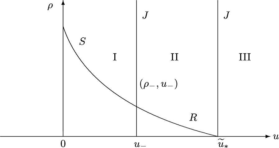
In the phase plane , through a given point , we draw the elementary wave curves. We find that the elementary wave curves divide the quarter phase plane into three regions, , , and , where , see Fig. 1. According to the right state in the different regions, one can construct the unique global Riemann solution connecting two constant states as follows: (1) : , (2) : , (3) : (see Fig. 1), where “+” means “followed by”.
-plane.
Limit of Riemann solutions of the AR model (1.1)–(1.2)
In this section, we study the limiting behavior of the Riemann solutions of (1.1)–(1.2) with the assumption as γ tends to zero, that is, the formation of delta shock as in the case .
Formation of delta shock wave
For any fixed , when , namely , the Riemann solution of (1.1)–(1.2) is a shock wave S followed by a contact discontinuity J with the intermediate state besides two constant states and . They satisfy
and
where and are the propagation speeds of S and J, respectively. Then we have the following lemmas.
If , then by the continuity of , there exists a sequence such that
for some . Then substituting the sequence into the right hand side of (4.3), and taking the limit , we have
This contradicts with the assumption . Then we must have , which means .
If , then we can also get a contradiction when taking limit in (4.3). Hence or . By the condition , it is easy to see that .
Next taking the limit in (4.3), we have
from which we can get . The proof is completed. □
where.
From (4.1), (4.2) and Lemma 4.1, we immediately get
The proof is completed. □
Lemmas 4.1–4.2 show that when γ tends to zero, S and J coincide, the intermediate density becomes singular.
From the first equations of the Rankine–Hugoniot relation (3.5) for S and J, we have
and
By (4.6) + (4.7), we get
which implies that
The proof is completed. □
Lemma 4.3 shows that when , the limit of has the same singularity as a weighted Dirac delta function at .
It can be concluded from Lemmas 4.1–4.3 that, when , S and J coincide to form a new type of nonlinear hyperbolic wave, which is called as the delta shock wave in [40]. Compared with the Riemann solutions of (1.5), it is clear to see that the propagation speed and strength of the delta shock wave here are and , which are different from those of the classical one to the zero pressure gas dynamics (1.5).
Now, we give the following theorem which give a very nice depiction of the limit of Riemann solutions of (1.1) and (1.2) as in the case .
Let. For any fixed, assume thatis a Riemann solution containing a shock wave and a contact discontinuity of (
1.1
) and (
1.2
) with the Riemann initial data (
1.3
). Then, as,will converge toin the sense of distributions, and the singular parts of the limit functionsandare a δ-measure with weightsrespectively, where.
(1) Set . Then for any fixed , the Riemann solution containing a shock wave and a contact discontinuity of (1.1) and (1.2) can be written as
From (3.2), we have the following weak formulations:
for any .
(2) For the first integral on the left-hand side of (4.9), using the method of integration by parts, we can derive
Meanwhile, we have
Then, by Lemma 4.2–4.3, we can obtain
Hence taking the limit in (4.9) leads to
where , .
(3) Similarly, we can obtain for (4.10) that
and
which converges to
by Lemma 4.1–4.3.
(4) Finally, we study the limits of and depending on t as . Regarding t as a parameter, we can get from (4.11) that
Then multiplying (4.13) by t and taking integration, we have
in which by definition (2.3), we have
where
In the same way, we can derive from (4.12) that
where
The proof is completed. □
In this section, we construct the Riemann solutions of the perturbed Aw–Rascle model (1.7) with initial data (1.3).
The system (1.7) has two eigenvalues
with the corresponding right eigenvectors
satisfying () for and . Thus, this system is strictly hyperbolic and both characteristic fields are genuinely nonlinear for and where is sufficiently small, which means the associated waves are either shock waves or rarefaction waves.
Seeking the self-similar solution
the Riemann problem (1.7) and (1.3) is reduced to the following boundary value problem of the ordinary differential equations:
with .
For any smooth solution, system (5.2) can be written as
Besides the constant solution
it provides the 1-rarefaction wave
or the 2-rarefaction wave
Differentiating the second equation of (5.4) with respect to ρ yields
and
where , which mean that for , the rarefaction wave curve is monotonic decreasing and convex in the phase plane .
Moreover, by differentiating ρ and u with respect to ξ in the first equation of (5.4) and combining
we have
Hence, as for sufficiently small, we have , i.e., the set which can be joined to by 1-rarefaction wave is made up of the half-branch of with .
With the same way to compute , we can gain , , and , which mean that it is monotonic creasing and concave for in the phase plane and the set which can be joined to by 2-rarefaction wave is made up of the half-branch of with .
Performing the limit in the second equation in (5.4) yields
Then we have
Thus we conclude that there exists such that the 1-rarefaction wave curve intersects the u-axis at the point .
Performing the limit of the second equation in (5.5) yields
which implies that
For a bounded discontinuity at , the Rankine–Hugoniot relation
holds, where , etc. Eliminating σ from (5.9), we obtain
Simplifying (5.10) yields
i.e.,
Therefore,
Set . Then (5.12) can be simplified as
This is a quadratic form in α and we can solve this to obtain
where and are the shock speed, the left state and the right state, respectively.
1-shock wave:
The classical Lax entropy conditions imply that the propagation speed for the 1-shock wave has to be satisfied with
From the first equation of (5.9), we have
Then, it follows from the right inequality of (5.14) that
which implies that and have different signs. Similarly, for the left inequality of (5.14), we can gain
Combining (5.15) and (5.16), it is easy to get
which indicates that , , and the minus sign is taken in (5.13) for 1-shock wave. Hence given a left state , the 1-shock wave curve in the phase plane which is the set of states that can be connected on the right by a 1-shock is as follows
2-shock wave:
The propagation speed for the 2-shock wave should satisfy
With the similar calculations to the 1-shock wave, we have the 2-shock curve :
Differentiating u with respect to ρ in the second equation of (5.11) gives that for ,
where
which gives for where sufficiently small, which indicates that the 1-shock wave curve is monotonic decreasing in the region in the phase plane. Moreover, letting in (5.11), it is easy to get
Setting
Then , and is continuous with respect to ρ. Therefore, there exists such that , which implies that the 1-shock wave curve intersects with the ρ-axis at a point.
Similarly, we can get for the 2-shock wave for where sufficiently small, which indicates that the 2-shock wave curve is monotonic increasing in the region in the phase plane. From (5.19), it is not difficult to check that for the 2-shock wave curve , which implies that curve has the u-axis as its asymptotic line.
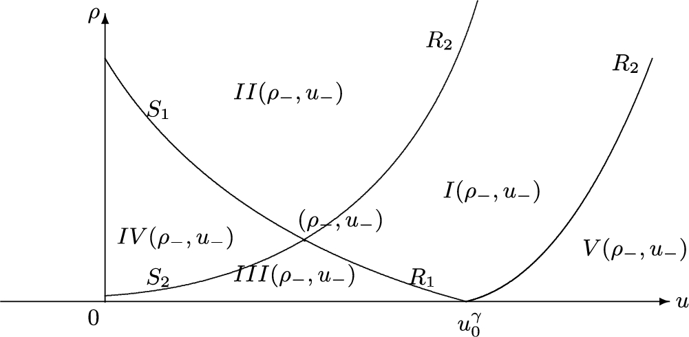
In the phase plane , through a given point , we draw the elementary wave curves. We find that the elementary wave curves divide the quarter phase plane into five regions, see Fig. 2. According to the right state in the different regions, one can construct the unique global solution to the Riemann problem (1.7) and (1.3) as follows:
In this section, we study the limiting behavior of the Riemann solutions of (1.7) as γ goes to one, that is, the formation of delta shock and the vacuum states as , respectively in the case and in the case .
Formation of delta shock wave
In this subsection, we study the formation of δ-shock in the Riemann problem (1.7) and (1.3) when as .
If, then there is a sufficiently smallsuch thatas.
If , then for any . Thus, we only need to consider the case .
It can be derived from (5.17) and (5.19) that all possible states that can be connected to the left state on the right by a 1-shock wave or a 2-shock wave should satisfy
If and , then from Fig. 1, (6.1) and (6.2), we have
which implies that
Since
it follows that there exists small enough such that, when , we have
Then, it is obvious that when . The proof is completed. □
According to the relation (5.11), for a given state , the shock curves and can also be expressed as below:
with for a 1-shock curve , and for a 2-shock curve .
When , namely , suppose that is the intermediate state connected with by a 1-shock wave with the speed , and by a 2-shock wave with the speed , then it follows from (6.7) that
with the shock speed
respectively. In this case, the Riemann solution is
If , then by the continuity of , there exists a sequence such that
for some . Then substituting the sequence into the right hand side of (6.12), taking the limit , and noting in mind, we have
Thus, we can obtain from (6.12) that
which contradicts with the assumption . Then we must have , which means .
If , then we can also get a contradiction when taking limit in (6.12). Hence or . By the condition , it is easy to see that .
Next taking the limit in (6.12), we have
from which we can get . The proof is completed. □
andwhere.
From (6.8)–(6.10) and Lemma 6.2, we immediately get
and
From the first equations of the Rankine–Hugoniot relation (5.9) for and , we have
and
By (6.14), (6.16) and (6.17), we get
which implies that
The proof is completed. □
Lemmas 6.2–6.3 show that when γ tends to one, the two shock curves and coincide to form a new delta shock wave, and the delta shock wave speed σ is the limit of both the particle velocity and two shocks’ speed , . What is more, the intermediate density tend to singular as .
What is more, we will further derive that, when , the limit of Riemann solutions of (1.7) with the Riemann initial data (1.3) under the assumption is a delta shock wave solution of the zero pressure gas dynamics (1.5) with the same Riemann initial data in the sense of distributions.
Let. For any fixed, assume thatis a Riemann solution containing two shocksandof (
1.7
) with the Riemann initial data (
1.3
) constructed in Section
5
. Then, as,will converge toin the sense of distributions, and the singular parts of the limit functionsandare a δ-measure with weightsrespectively, which form a delta shock solution of (
1.5
) with the same Riemann data (
1.3
). Here.
(1) Set . Then for any fixed , the Riemann solution containing two shocks and of (1.7) with the Riemann initial data (1.3) can be written as
From (5.2), we have the following weak formulations:
for any .
(2) For the first integral on the left-hand side of (6.19), using the method of integration by parts, we can derive
Meanwhile, we have
Then, by Lemma 6.2–6.3, we can obtain
Hence taking the limit in (6.19) leads to
where , .
(3) Similarly, we can obtain for (6.20) that
and
which converges to
by Lemma 6.2–6.3.
(4) Finally, we study the limits of and depending on t as . Regarding t as a parameter, we can get from (6.21) that
Then multiplying (6.23) by t and taking integration, we have
in which by definition (2.3), we have
where
In the same way, we can derive from (6.22) that
where
The proof is completed. □
Numerical simulations
In this section, we use the fifth-order weighted essentially non-oscillatory scheme and third-order Runge–Kutta method [16,35] with the mesh 400 points to present two selected groups of representative numerical simulations for the Aw–Rascle traffic model (1.1)–(1.2) and the perturbed Aw–Rascle model (1.7) as γ decreases. A number of iterative numerical trials are executed to guarantee what we demonstrate are not numerical objects. The numerical simulations are consistent with the theoretical analysis.
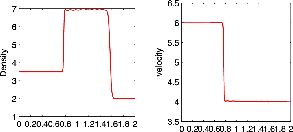
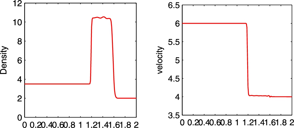
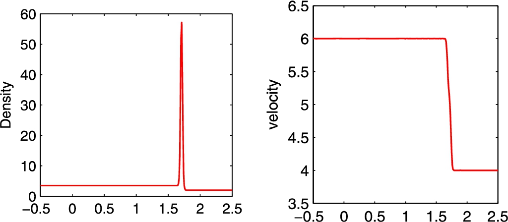
The numerical simulations are corresponding to the theoretical analysis in Section 4. When , we take the initial data as follows:
and compute the solution of the Riemann problem of (1.1)–(1.2) up to , the numerical simulations for different choices of γ, starting with , then , and finally , are presented in Figs 3–5 which show the process of concentration and formation of the delta shock wave in vanishing adiabatic exponent limit of solutions containing a shock wave and a contact discontinuity.
Density (left) and velocity (right) for .
Density (left) and velocity (right) for .
Density (left) and velocity (right) for .
From these numerical results, we can clearly observe that, when γ decreases, the locations of the shock wave and contact discontinuity become closer and closer, and the density of the intermediate state increases dramatically, while the velocity becomes a piecewise constant function. In the end, as , along with the intermediate state, the shock wave and the contact discontinuity coincide to form a delta-shock, while the velocity keeps a step function. The numerical simulations are in complete agreement with the theoretical analysis in Section 4.
What’s more, by Theorem 4.4 and (4.1)–(4.2), if , then the solution of the Riemann problem (1.1)–(1.2) with the Riemann initial data can be expressed as
where
and the state is determined uniquely by
From (7.5), the solution will be computed by
Then we compute by using the first equation in (7.5) and compute () by using (7.3)–(7.4) and the time . Thus, for , we can calculate that
Similarly, for ,
And for ,
The numerical methods for the Aw–Rascle traffic model are in complete agreement with the theoretical analysis in Section 4.
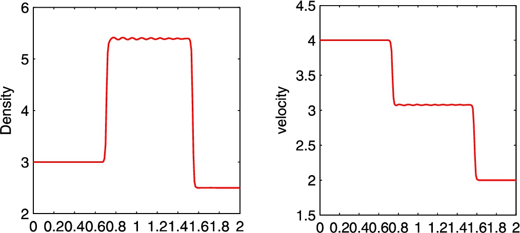
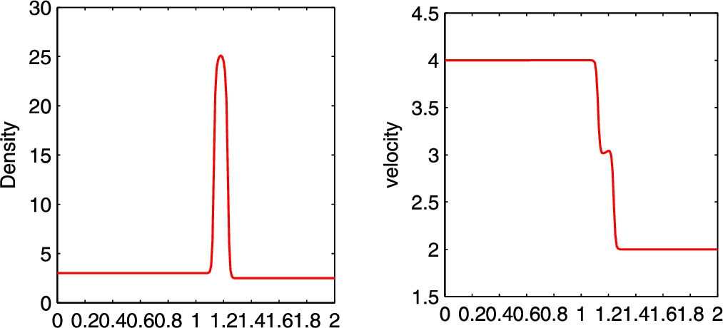
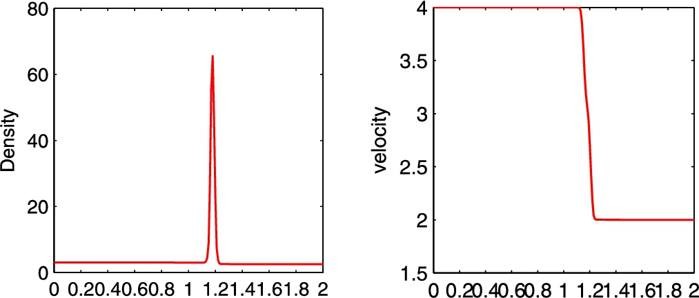
The numerical simulations are corresponding to the theoretical analysis in Section 6. When , we take the initial data as follows:
and compute the solution of the Riemann problem of (1.7) up to , the numerical simulations for different choices of γ, starting with , then , and finally , are presented in Figs 6–8 which show the process of concentration and formation of the delta shock wave in the pressureless limit of solutions containing two shocks.
Density (left) and velocity (right) for .
Density (left) and velocity (right) for .
Density (left) and velocity (right) for .
From these numerical results, we can clearly observe that, as γ decreases, the locations of the two shocks become closer and closer, and the density of the intermediate state increases dramatically, while the velocity becomes a piecewise constant function. In the end, as , along with the intermediate state, the two shocks coincide to form the delta shock wave of the zero pressure gas dynamics (1.5), while the velocity keeps a step function. The numerical simulations are in complete agreement with the theoretical analysis in Section 6.
What’s more, by Theorem 6.4, (6.1)–(6.2) and (6.10), if , then the solution of the Riemann problem (1.7) with the Riemann initial data can be expressed as
where
and the state is determined uniquely by
Because these Eqs (7.13)–(7.14) are too complex to be solved exactly. By (7.13) + (7.14), we have
where is substituted by (7.13). Hence, the Eq. (7.15) is about . To obtain approximate solution , we compute (7.15) by using numerical methods on MATLAB. Then we compute by using the Eq. (7.13) and compute () by using (7.12) and the time . Thus, for , we can calculate that
Similarly, for ,
And for ,
The numerical methods are in complete agreement with the theoretical analysis in Section 6.
Conclusion
The phenomenon of concentration and the formation of delta shock wave in vanishing adiabatic exponent limit of the solutions of Riemann problem to the Aw–Rascle traffic model is investigated in this paper. We find that as the adiabatic exponent vanishes, the limit of Riemann solutions tends to a special delta shock wave rather than the classical one to the zero pressure gas dynamics. In order to further study this problem, we consider a perturbed Aw–Rascle model and proceed to investigate the limit of Riemann solutions. We rigorously proved that, as the adiabatic exponent tends to one, any Riemann solution containing two shock waves tends to a delta-shock to the zero pressure gas dynamics in the distribution sense. The paper is also supplemented with numerical experiments to illustrate the presented solution behaviors. Compared to the vanishing pressure limit method, the method of letting adiabatic exponent tend to zero is called as the zero-exponent limit method or vanishing adiabatic exponent limit method. Using this method, we in this paper study vanishing adiabatic exponent limit of the solutions of Riemann problem to the Aw–Rascle traffic model. Our results, to a certain extent, extend the previous research works [23,31,42] on vanishing pressure limit of Riemann solutions to the Aw–Rascle model. The results obtained to some extent provide us a new different mathematical analysis to study the formation of delta shock wave arising in the Aw–Rascle traffic model, which is just the novelty of this paper lies in. Currently, the mathematical study of solutions to hyperbolic systems with a Coulomb-like friction term is active. Thus, it is natural and interesting to study the limit of Riemann solutions to the Aw–Rascle traffic model with source term, such as the friction, damping and relaxation effect. We leave this problem for our future work.
Footnotes
Acknowledgements
The authors are very grateful to the anonymous referees for their valuable comments and corrections, which have improved the original manuscript greatly. This work is supported by the Natural Science Foundation of Fujian Province of China (Grant No. 2019J01642) and the Research Foundation of Fuzhou University (Grant No. FDJG20190027).
References
1.
A.Aw and M.Rascle, Resurrection of “second order” models of traffic flow, SIAM J. Appl. Math.60 (2000), 916–938. doi:10.1137/S0036139997332099.
2.
F.Bouchut, On zero pressure gas dynamics, in: Advances in Kinetic Theory and Computing, Ser. Adv. Math. Appl. Sci., Vol. 22, World Scientific Publishing, River Edge, NJ, 1994, pp. 171–190.
3.
Y.Brenier and E.Grenier, Sticky particles and scalar conservation laws, SIAM J. Numer. Anal.35 (1998), 2317–2328. doi:10.1137/S0036142997317353.
4.
R.K.Chaturvedi and L.P.Singh, The phenomena of concentration and cavitation in the Riemann solution for the isentropic zero-pressure dusty gasdynamics, Journal of Mathematical Physics62 (2021), 033101. doi:10.1063/5.0023511.
5.
G.-Q.Chen and H.Liu, Concentration and cavitation in the vanishing pressure limit of solutions to the Euler equations for nonisentropic fluids, Phys. D189 (2004), 141–165. doi:10.1016/j.physd.2003.09.039.
6.
G.Q.Chen and H.Liu, Formation of δ-shocks and vacuum states in the vanishing pressure limit of solutions to the Euler equations for isentropic fluids, SIAM J. Math. Anal.34 (2003), 925–938. doi:10.1137/S0036141001399350.
7.
H.Cheng and H.Yang, Approaching Chaplygin pressure limit of solutions to the Aw–Rascle model, J. Math. Anal. Appl.416 (2014), 839–854. doi:10.1016/j.jmaa.2014.03.010.
8.
C.Daganzo, Requiem for second order fluid approximations of traffic flow, Transportation Res. Part B29 (1995), 277–286. doi:10.1016/0191-2615(95)00007-Z.
9.
W.E, Yu.G.Rykov and Ya.G.Sinai, Generalized variational principles, global weak solutions and behavior with random initial data for systems of conservation laws arising in adhesion particle dynamics, Comm. Math. Phys.177 (1996), 349–380. doi:10.1007/BF02101897.
10.
L.Guo, T.Li and G.Yin, The vanishing pressure limits of Riemann solutions to the Chaplygin gas equations with a source term, Commun. Pure Appl. Anal.16(1) (2017), 295–309. doi:10.3934/cpaa.2017014.
11.
L.Guo, T.Li and G.Yin, The limit behavior of the Riemann solutions to the generalized Chaplygin gas equations with a source term, J. Math. Anal. Appl.455(1) (2017), 127–140. doi:10.1016/j.jmaa.2017.05.048.
12.
S.Ha, F.Huang and Y.Wang, A global unique solvability of entropic weak solution to the one-dimensional pressureless Euler system with a flocking dissipation, J. Differ. Equations257 (2014), 1333–1371. doi:10.1016/j.jde.2014.05.007.
13.
F.Huang and Z.Wang, Well posedness for pressureless flow, Comm. Math. Phys.222 (2001), 117–146. doi:10.1007/s002200100506.
14.
M.Ibrahim, F.Liu and S.Liu, Concentration of mass in the pressureless limit of Euler equations for power law, Nonlinear Anal. Real World Appl.47 (2019), 224–235. doi:10.1016/j.nonrwa.2018.10.015.
15.
K.T.Joseph, A Riemann problem whose viscosity solutions contain δ-measures, Asymptot Anal.7 (1993), 105–120. doi:10.3233/ASY-1993-7203.
16.
A.Kurganov and E.Tadmor, New high-resolution central schemes for nonlinear conservation laws and convection diffusion equations, J. Comput. Phys.160 (2000), 241–282. doi:10.1006/jcph.2000.6459.
17.
J.Lebacque, S.Mammar and H.Salem, The Aw–Rascle and Zhang’s model: Vacuum problems, existence and regularity of the solutions of the Riemann problem, Transp. Res. Part B41 (2007), 710–721. doi:10.1016/j.trb.2006.11.005.
18.
H.Li and Z.Shao, Delta shocks and vacuum states in vanishing pressure limits of solutions to the relativistic Euler equations for generalized Chaplygin gas, Commun. Pure Appl. Anal.15 (2016), 2373–2400. doi:10.3934/cpaa.2016041.
19.
H.Li and Z.Shao, Vanishing pressure limit of Riemann solutions to the Aw–Rascle model for generalized Chaplygin gas, Acta Mathematica Scientia37A (2017), 917–930.
20.
J.Li, Note on the compressible Euler equations with zero temperature, Appl. Math. Lett.14 (2001), 519–523. doi:10.1016/S0893-9659(00)00187-7.
21.
J.Li and H.Yang, Delta-shocks as limits of vanishing viscosity for multidimensional zero-pressure gas dynamics, Quart. Appl. Math.59(2) (2001), 315–342. doi:10.1090/qam/1827367.
22.
J.Li, T.Zhang and S.Yang, The Two-Dimensional Riemann Problem in Gas Dynamics, Pitman Monographs and Surveys in Pure and Applied Mathematics, Vol. 98, Longman, Harlow, 1998.
23.
J.Liu and W.Xiao, Flux approximation to the Aw–Rascle model of traffic flow, Journal of Mathematical Physics59 (2018), 101508. doi:10.1063/1.5063469.
24.
Y.Liu and W.Sun, Wave interactions and stability of Riemann solutions of the Aw–Rascle model for generalized Chaplygin gas, Acta Applicandae Mathematicae154 (2018), 95–109. doi:10.1007/s10440-017-0135-0.
25.
Y.Liu and W.Sun, The perturbed Riemann problem for the Aw–Rascle model with modified Chaplygin gas pressure, Advances in Mathematical Physics2018 (2018), 7104527. doi:10.1155/2018/8702152.
26.
D.Mitrovic and M.Nedeljkov, Delta-shock waves as a limit of shock waves, J. Hyperbolic Differ. Equ.4 (2007), 629–653. doi:10.1142/S021989160700129X.
27.
L.Pan and X.Han, The Aw–Rascle traffic model with Chaplygin pressure, J. Math. Anal. Appl.401 (2013), 379–387. doi:10.1016/j.jmaa.2012.12.022.
28.
S.F.Shandarin and Ya.B.Zeldovich, The large-scale structure of the universe: Turbulence, intermittency, structures in a self-gravitating medium, Rev. Modern Phys.61 (1989), 185–220. doi:10.1103/RevModPhys.61.185.
29.
C.Shen, The limits of Riemann solutions to the isentropic magnetogasdynamics, Appl. Math. Lett.24 (2011), 1124–1129. doi:10.1016/j.aml.2011.01.038.
30.
C.Shen, W.Sheng and M.Sun, The asymptotic limits of solutions to the Riemann problem for the scaled Leroux system, Commun. Pure Appl. Anal.17 (2018), 391–411. doi:10.3934/cpaa.2018022.
31.
C.Shen and M.Sun, Formation of delta shocks and vacuum states in the vanishing pressure limit of Riemann solutions to the perturbed Aw–Rascle model, J. Differential Equations249 (2010), 3024–3051. doi:10.1016/j.jde.2010.09.004.
32.
C.Shen, M.Sun and Z.Wang, Limit relations for three simple hyperbolic systems of conservation laws, Math. Meth. Appl. Sci.33 (2010), 1317–1330. doi:10.1002/mma.1248.
33.
W.Sheng, G.Wang and G.Yin, Delta wave and vacuum state for generalized Chaplygin gas dynamics system as pressure vanishes, Nonlinear Anal. Real World Appl.22 (2015), 115–128. doi:10.1016/j.nonrwa.2014.08.007.
34.
W.Sheng and T.Zhang, The Riemann Problem for the Transportation Equations in Gas Dynamics, Mem. Amer. Math. Soc., Vol. 137, AMS, Providence, 1999.
35.
C.W.Shu, Essentially non-oscillatory and weighted essentially non-oscillatory schemes for hyperbolic conservation laws, in: Advanced Numerical Approximation of Nonlinear Hyperbolic Equations, Lecture Notes in Mathematics, Vol. 1697, Springer, Berlin Heidelberg, 1998, pp. 325–432. doi:10.1007/BFb0096355.
36.
M.Sun, Interactions of elementary waves for the Aw–Rascle model, SIAM J. Appl. Math.69 (2009), 1542–1558, 21. doi:10.1137/080731402.
37.
M.Sun, A note on the interactions of elementary waves for the AR traffic flow model without vacuum, Acta Math. Sci.31(B) (2011), 1503–1512.
38.
M.Sun, The limits of Riemann solutions to the simplified pressureless Euler system with flux approximation, Mathematical Methods in the Applied Sciences41 (2018), 4528–4548. doi:10.1002/mma.4912.
39.
M.Sun, Concentration and cavitation phenomena of Riemann solutions for the isentropic Euler system with the logarithmic equation of state, Nonlinear Anal Real World Appl.53 (2020), 103068. doi:10.1016/j.nonrwa.2019.103068.
40.
M.Tong and C.Shen, The limits of Riemann solutions for the isentropic Euler system with extended Chaplygin gas, Applicable Analysis98 (2019), 2668–2687. doi:10.1080/00036811.2018.1469009.
41.
M.Tong, C.Shen and X.Lin, The asymptotic limits of Riemann solutions for the isentropic extended Chaplygin gas dynamic system with the vanishing pressure, Boundary Value Problems2018 (2018), 144. doi:10.1186/s13661-018-1064-1.
42.
J.Wang, J.Liu and H.Yang, Vanishing pressure limit of solutions to the Aw–Rascle model for modified Chaplygin gas, 2014, https://arxiv.org/abs/1410.1110.
43.
H.Yang and J.Wang, Concentration in vanishing pressure limit of solutions to the modified Chaplygin gas equations, Journal of Mathematical Physics57 (2016), 111504. doi:10.1063/1.4967299.
44.
G.Yin and J.Chen, Existence and stability of Riemann solution to the Aw–Rascle model with friction, Indian Journal of Pure and Applied Mathematics49 (2018), 671–688. doi:10.1007/s13226-018-0294-3.
45.
G.Yin and W.Sheng, Delta shocks and vacuum states in vanishing pressure limits of solutions to the relativistic Euler equations for polytropic gases, J. Math. Anal. Appl.355 (2009), 594–605. doi:10.1016/j.jmaa.2009.01.075.
46.
H.Zhang, A non-equilibrium traffic model devoid of gas-like behavior, Transportation Res. Part B36 (2002), 275–290. doi:10.1016/S0191-2615(00)00050-3.
47.
Q.Zhang, Concentration in the flux approximation limit of Riemann solutions to the extended Chaplygin gas equations with friction, Journal of Mathematical Physics60 (2019), 101508. doi:10.1063/1.5085233.
48.
Y.Zhang and M.Sun, Concentration phenomenon of Riemann solutions for the relativistic Euler equations with the extended Chaplygin gas, Acta Appl Math170 (2020), 539–568. doi:10.1007/s10440-020-00345-7.
49.
Y.Zhang and J.Wang, The limits of Riemann solutions to the relativistic van der Waals fluid, Applicable Analysis (2019). doi:10.1080/00036811.2019.1705284.
50.
Y.Zhang and Y.Zhang, Delta-shocks and vacuums in the relativistic Euler equations for isothermal fluids with the flux approximation, Journal of Mathematical Physics60 (2019), 011508. doi:10.1063/1.5001107.
51.
Y.Zhang, Y.Zhang and J.Wang, Concentration in the zero-exponent limit of solutions to the isentropic Euler equations for extended Chaplygin gas, Asymptotic Analysis122 (2021), 35–67. doi:10.3233/ASY-201609.