Stability analysis of laminated beams with Kelvin–Voigt damping and strong time delay

Abstract

In this paper we consider a model of laminated beams combining viscoelastic damping and strong time-delayed damping. The global well-posedness is proved by using the theory of semigroups of linear operators. We prove the lack of exponential stability when the speed wave propagations are not equal. In fact, we show in this situation, that the system goes to zero polynomially with rate $t^{- 1 / 2}$ . On the other hand, by constructing some suitable multipliers, we establish that the energy decays exponentially provided the equal-speed wave propagations hold.

Keywords

Laminated beams Kelvin–Voigt damping strong delay exponential decay polynomial decay

1. Introduction

In this work, we are interested in studying the following laminated beams with strong time delay in $(x, t) \in (0, l) \times [0, \infty)$ , $\begin{array}{rcl} (1.1) & \begin{array}{l} ρ u_{t t} + G {(ψ - u_{x})}_{x} = 0, \\ I_{ρ} {(3 S - ψ)}_{t t} - D {(3 S - ψ)}_{x x} - G (ψ - u_{x}) - μ_{1} {(3 S - ψ)}_{x x t} \\ - μ_{2} {(3 S - ψ)}_{x x t} (x, t - τ) = 0, \\ 3 I_{ρ} S_{t t} - 3 D S_{x x} + 3 G (ψ - u_{x}) + 4 δ S + 4 γ S_{t} = 0, \end{array} \end{array}$ subject to boundary conditions given by $\begin{array}{rcl} (1.2) & u (0, t) = ψ_{x} (0, t) = S_{x} (0, t) = u_{x} (l, t) = ψ (l, t) = S (l, t) = 0 in (0, \infty) \end{array}$ and initial conditions $\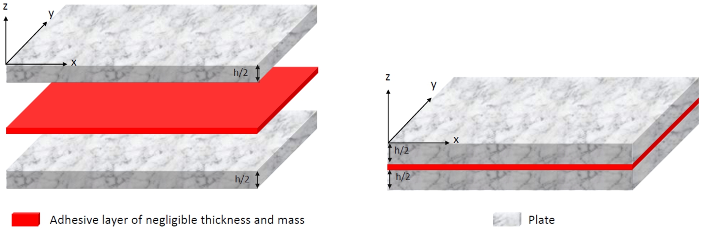begin{array}{rcl} (1.3) & \begin{array}{l} u (x, 0) = u_{0} (x), u_{t} (x, 0) = u_{1} (x), ψ (x, 0) = ψ_{0} (x), x \in (0, l), \\ ψ_{t} (x, 0) = ψ_{1} (x), S (x, 0) = S_{0} (x), S_{t} (x, 0) = S_{1} (x), x \in (0, l), \\ {(3 S - ψ)}_{x x t} (x, t - τ) = f_{0} (x, t - τ), (x, t) \in (0, l) \times (0, τ) . \end{array} \end{array}$

The laminated beam is a mathematical model given by two plates connected by an adhesive layer of negligible thickness and mass. An example of applying an adhesive to glue two plates (layers) is shown in Fig. 1.

Fig. 1.

Adhesive application (left) and plate in the press (right).

The model was derived from Timoshenko’s theory by S. Hansen and R. Spies [15,16] and is given by the following three equations $\begin{array}{rcl} (1.4) & \begin{array}{l} ρ ω_{t t} + G {(ψ - ω_{x})}_{x} = 0, \\ I_{ρ} (3 s_{t t} - ψ_{t t}) - G (ψ - ω_{x}) - D (3 s_{x x} - ψ_{x x}) = 0, \\ I_{ρ} s_{t t} + G (ψ - ω_{x}) + \frac{4}{3} γ s + \frac{4}{3} β s_{t} - D s_{x x} = 0, \end{array} \end{array}$ where the coefficients ρ, G, $I_{ρ}$ , D, γ, β are positive constants and represent density, shear stiffness, mass moment of inertia, flexural rigidity, adhesive stiffness, and adhesive damping parameter, respectively. The function $ω (x, t)$ is the transversal displacement, $ψ (x, t)$ is the rotational displacement and $s (x, t)$ is proportional to the amount of slip along the interface. The third equation describes the dynamics of the slip.

For laminated beams without time delay, we start citing the contribution in [36], where the authors considered (1.4) with the following boundary control, $\begin{array}{l} ψ (1) - ω_{x} (1) = k_{1} ω_{t} (1), s_{x} (1) = 0, (3 s_{x} - ψ_{x}) (1) = - k_{2} (3 s_{t} - ψ_{t}) (1), \end{array}$ and obtained that the energy decays exponentially by assuming $k_{i} \neq r_{i}$ , $(i = 1, 2)$ , where $\begin{array}{rcl} r_{1} : = \frac{G}{ρ} \neq \frac{D}{I_{ρ}} : = r_{2} . \end{array}$ This result was improved by Mustafa, who established the exponential decay for $r_{1} = r_{2}$ and extended these results to cases of nonlinear functions in the boundary control, see [25]. We can also find some stability results on the system (1.4) with boundary damping in [7,33,35], etc. Raposo [32] investigated (1.4) by adding frictional damping terms on the transverse displacement and rotation angle, respectively. He established the exponential stability of the system without any restrictions on the coefficients. The result was extended to a nonlinear framework by Feng et al. [12]. More results on (1.4) with other kind of damping mechanisms, one can refer to [1,2,8,21,22,26] to cite but a few.

The delay effects often appear in many practical problems, for instance, chemical, physical, thermal and economic phenomena, and so on, and the presence of an arbitrarily small delay may destabilize a system which is uniformly or asymptotically stable in the absence of delay. For example, Nicaise and Pignotti [27] considered the system $\begin{matrix} u_{t t} - Δ u = 0, & x \in Ω, t > 0, \\ u = 0, & x \in Γ_{0}, t > 0, \\ \frac{\partial u}{\partial ν} + μ_{1} u_{t} (t) + μ_{2} u_{t} (t - τ) = 0, & x \in Γ_{1}, t > 0, \end{matrix}$ and proved that the energy decays exponentially under the assumption $μ_{2} < μ_{1}$ , otherwise the system is unstable. Similar results can be found in [28,29].

For laminated beams with time delay, there are few results. Feng [11] studied system (1.4) with three internal constant time delays and boundary feedback. He proved that the system is exponentially stable if the coefficients of time delay are small. Mpungu et al. [24] considered (1.4) with frictional damping and an internal constant delay term in the transverse displacement. They obtained the system is exponentially stable if the assumption of equal wave speeds holds, otherwise, the energy decays polynomially. Choucha et al. [9] studied a thermoelastic laminated Timoshenko beam with distributed delay. They proved the same stability results as in [24]. Note that the system (1.4) reduces to Timoshenko system if $s = 0$ . Said-Houari and Laskri [34] investigated a Timoshenko system with a delay of the form $\begin{array}{l} ρ_{1} φ_{t t} - κ {(φ_{x} + ψ)}_{x} = 0, \\ ρ_{2} ψ_{t t} - b ψ_{x x} + κ (φ_{x} + ψ) + μ_{1} ψ_{t} + μ_{2} ψ_{t} (t - τ) = 0, \end{array}$ and established the exponential energy decay provided $μ_{2} < μ_{1}$ . The result was extended by Kirane et al. to the case of the time-varying delay, see [20]. Makheloufi et al. [23] studied a Timoshenko system with a strong damping and a strong delay given by $\begin{array}{l} ρ_{1} φ_{t t} - κ {(φ_{x} + ψ)}_{x} - μ_{1} φ_{x x t} - μ_{2} φ_{x x t} (t - τ) = 0, \\ ρ_{2} ψ_{t t} - b ψ_{x x} + κ (φ_{x} + ψ) = 0 . \end{array}$ They proved that the system is not exponentially stable even if the equal-speed wave propagations hold. For more results on stability of Timoshenko with time delay, one can refer to [3,10,14,18], etc.

Motivated by the above scenario, in the present paper, we consider the laminated beams with strong time delay $μ_{2} {(3 S - ψ)}_{x x t} (x, t - τ)$ . We aim to study the well-posedness and results of stability for the system taking into account the stability number $\begin{matrix} χ : = \frac{G}{ρ} - \frac{D}{I_{ρ}} . \end{matrix}$ The well-posedness is proved by semigroup of linear operators, see Section 2. In Section 3, by using the Gearhart-Herbst-Prüss-Huang Theorem, we prove that system (1.1)–(1.3) is not exponentially stable if $χ \neq 0$ . Finally, the Section 4 is devoted to energy decay of the system, where we prove that the energy decays exponentially in the case of equal wave speeds of propagation, that is, $χ = 0$ . Otherwise, if $χ \neq 0$ , the system goes to zero polynomially with rate $t^{- 1 / 2}$ .

2. Well-posedness

We introduce a new dependent variable z to deal with the delay feedback term, i.e., $\begin{array}{rcl} (2.1) & z (x, η, t) = {(3 S - ψ)}_{t} (x, t - η τ) in (0, l) \times (0, 1) \times (0, \infty) . \end{array}$ It is easily verified that the z satisfies $\begin{array}{rcl} (2.2) & τ z_{t} (x, η, t) + z_{η} (x, η, t) = 0 in (0, l) \times (0, 1) \times (0, \infty) . \end{array}$ Following the idea of [36], we denote the effective rotation angle by $ξ : = 3 S - ψ$ . By (2.2), the differential equations (1.1) can be rewritten as follows: $\begin{array}{rcl} (2.3) & \begin{array}{l} ρ u_{t t} + G {(3 S - ξ - u_{x})}_{x} = 0 in (0, l) \times (0, \infty), \\ I_{ρ} ξ_{t t} - D ξ_{x x} - G (3 S - ξ - u_{x}) - μ_{1} ξ_{x x t} - μ_{2} z_{x x} (x, 1, t) = 0 in (0, l) \times (0, \infty), \\ 3 I_{ρ} S_{t t} - 3 D S_{x x} + 3 G (3 S - ξ - u_{x}) + 4 δ S + 4 γ S_{t} = 0 in (0, l) \times (0, \infty), \\ τ z_{t} (x, η, t) + z_{η} (x, η, t) = 0 in (0, l) \times (0, 1) \times (0, \infty), \end{array} \end{array}$ subject to boundary conditions given in (1.2), that is, $\begin{array}{rcl} (2.4) & u (0, t) = ξ_{x} (0, t) = S_{x} (0, t) = u_{x} (l, t) = ξ (l, t) = S (l, t) = 0 in (0, \infty) \end{array}$ and initial conditions $\begin{array}{rcl} (2.5) & \begin{array}{l} u (x, 0) = u_{0}, u_{t} (x, 0) = u_{1}, ξ (x, 0) = ξ_{0}, x \in (0, l), \\ ξ_{t} (x, 0) = ξ_{1}, S (x, 0) = S_{0}, S_{t} (x, 0) = S_{1}, x \in (0, l), \\ z (x, η, 0) = f_{0} (x, - η τ) = ξ_{2} (x, η), (x, η) \in (0, l) \times (0, 1) . \end{array} \end{array}$

In the following, using the semigroup theory found in [30], a result of existence, uniqueness and regularity will be obtained for the problem (2.3)–(2.5).

Now, consider the following Hilbert space: $\begin{array}{rcl} (2.6) & \begin{array}{l} H = H_{a}^{1} (0, l) \times L^{2} (0, l) \times H_{b}^{1} (0, l) \times L^{2} (0, l) \times H_{b}^{1} (0, l) \\ \times L^{2} (0, l) \times H_{b}^{1} ((0, l); L^{2} (0, 1)), \end{array} \end{array}$ where $\begin{array}{rcl} (2.7) & \begin{array}{l} H_{a}^{1} (0, l) = {φ : φ \in H^{1} (0, l), φ (0) = 0} and H_{b}^{1} (0, l) = {φ : φ \in H^{1} (0, l), φ (l) = 0} . \end{array} \end{array}$ For ζ a positive constant satisfying $\begin{array}{rcl} (2.8) & τ | μ_{2} | ⩽ ζ ⩽ τ (2 μ_{1} - | μ_{2} |), \end{array}$ the inner product on $H$ is $\begin{array}{rcl} (2.9) & \begin{array}{l} {⟨ U, U^{*} ⟩}_{H} = ρ \int_{0}^{l} w \overline{w^{*}} d x + G \int_{0}^{l} (3 S - ξ - u_{x}) \overline{(3 S^{*} - ξ^{*} - u_{x}^{*})} d x + I_{ρ} \int_{0}^{l} v \overline{v^{*}} d x \\ + D \int_{0}^{l} ξ_{x} \overline{ξ_{x}^{*}} d x + 3 I_{ρ} \int_{0}^{l} y \overline{y^{*}} d x + 3 D \int_{0}^{l} S_{x} \overline{S_{x}^{*}} d x \\ + 4 δ \int_{0}^{l} S \overline{S^{*}} d x + ζ \int_{0}^{l} \int_{0}^{1} z_{x} \overline{z_{x}^{*}} d η d x, \end{array} \end{array}$ for any $U = (u, w, ξ, v, S, y, z)$ , $U^{*} = (u^{*}, w^{*}, ξ^{*}, v^{*}, S^{*}, y^{*}, z^{*})$ in $H$ . The norm induced by the inner product is $\begin{array}{rcl} (2.10) & \begin{array}{l} ‖ U ‖_{H} = ρ ‖ w ‖^{2} + G ‖ 3 S - ξ - u_{x} ‖^{2} + I_{ρ} ‖ v ‖^{2} + D ‖ ξ_{x} ‖^{2} + 3 I_{ρ} ‖ y ‖^{2} \\ + 3 D ‖ S_{x} ‖^{2} + 4 δ ‖ S ‖^{2} + ζ \int_{0}^{1} ‖ z_{x} ‖^{2} d η . \end{array} \end{array}$ Introducing $U (t) = {(u (t), u_{t} (t), ξ (t), ξ_{t} (t), S (t), S_{t} (t), z (t))}^{⊤}$ and $U_{0} = {(u_{0}, u_{1}, ξ_{0}, ξ_{1}, S_{0}, S_{1}, ξ_{2})}^{⊤}$ , the system (2.3)–(2.5) can be written as the following abstract initial value problem in $H$ $\begin{array}{rcl} (2.11) & \{\begin{matrix} U_{t} (t) = A U (t), & t > 0, \\ U (0) = U_{0}, \end{matrix} \end{array}$ where the operator $A : D (A) \subset H \to H$ is given by $\begin{array}{rcl} (2.12) & A (\begin{matrix} u \\ w \\ ξ \\ v \\ S \\ y \\ z \end{matrix}) = (\begin{matrix} w \\ - G ρ^{- 1} {(3 S - ξ - u_{x})}_{x} \\ v \\ I_{ρ}^{- 1} (D ξ_{x x} + G (3 S - ξ - u_{x}) + μ_{1} v_{x x} + μ_{2} z_{x x} (\cdot, 1)) \\ y \\ I_{ρ}^{- 1} (D S_{x x} - G (3 S - ξ - u_{x}) - \frac{4}{3} δ S - \frac{4}{3} γ y) \\ - τ^{- 1} z_{η} \end{matrix}), \end{array}$ with $\begin{matrix} (2.13) & D (A) = \{\begin{matrix} U = {(u, w, ξ, v, S, y, z)}^{⊤} \in H : & \begin{matrix} u, S, D ξ + μ_{1} v + μ_{2} z (\cdot, 1) \in H^{2} (0, l), w \in H_{a}^{1} (0, l), \\ v, y \in H_{b}^{1} (0, l), z \in H_{b}^{1} ((0, l); H^{1} (0, 1)), \\ u_{x} (l) = ξ_{x} (0) = S_{x} (0) = z_{x} (0, \cdot) = 0 . \end{matrix} \end{matrix}\} . \end{matrix}$

Note that $D (A)$ is dense in $H$ and is easy to show that $A$ is dissipative since $| μ_{2} | < μ_{1}$ (for more details, see Theorem 4.2), and for each $U = {(u, w, ξ, v, S, y, z)}^{⊤} \in D (A)$ , we have $\begin{array}{rcl} (2.14) & Re {⟨ A U, U ⟩}_{H} ⩽ - K (‖ v_{x} ‖^{2} + ‖ y ‖^{2} + {‖ z_{x} (x, 1) ‖}^{2}), \end{array}$ where $K : = min {μ_{1} - \frac{| μ_{2} |}{2} - \frac{ζ}{2 τ}, \frac{ζ}{2 τ} - \frac{| μ_{2} |}{2}, 4 γ} > 0$ since (2.8) hold.

Our existence and uniqueness result reads as follows.

Theorem 2.1 (Existence and uniqueness).

Assume that $| μ_{2} | < μ_{1}$ , then for any $U_{0} \in H$ , there exists a unique solution $U \in C ([0, \infty), H)$ of problem ( 2.11 ). Moreover, if $U_{0} \in D (A)$ , then $\begin{array}{rcl} (2.15) & U \in C ([0, \infty), D (A)) \cap C^{1} ([0, \infty), H) . \end{array}$

Proof.
Since the operator $A$ is dissipative. Now, we will prove that operator $λ I - A$ is surjective for $λ > 0$ . For this purpose, let $F = {(f_{1}, f_{2}, \dots, f_{7})}^{⊤} \in H$ , we seek $U = {(u, w, ξ, v, S, y, z)}^{⊤} \in D (A)$ which is solution of $(λ I - A) U = F$ , that is, the entries of U satisfy the system of equations $\begin{array}{l} (2.16) & λ u - w = f_{1}, \\ (2.17) & λ ρ w + G {(3 S - ξ - u_{x})}_{x} = ρ f_{2}, \\ (2.18) & λ ξ - v = f_{3}, \\ (2.19) & λ I_{ρ} v - D ξ_{x x} - G (3 S - ξ - u_{x}) - μ_{1} v_{x x} - μ_{2} z_{x x} (x, 1) = I_{ρ} f_{4}, \\ (2.20) & λ S - y = f_{5}, \\ (2.21) & 3 λ I_{ρ} y - 3 D S_{x x} + 3 G (3 S - ξ - u_{x}) + 4 δ S + 4 γ y = 3 I_{ρ} f_{6}, \\ (2.22) & λ τ z + z_{η} = τ f_{7} . \end{array}$ Suppose that we have found u, ξ and S with the appropriated regularity. Therefore, from (2.16), (2.18) and (2.20) we have $\begin{array}{l} (2.23) & w = λ u - f_{1}, \\ (2.24) & v = λ ξ - f_{3}, \\ (2.25) & y = λ S - f_{5} . \end{array}$ It is clear that $w \in H_{a}^{1} (0, l)$ and $v, y \in H_{b}^{1} (0, l)$ . Furthermore, $\begin{array}{rcl} (2.26) & z (x, η) = v (x) e^{- λ τ η} + τ e^{- λ τ η} \int_{0}^{η} f_{7} (x, σ) e^{λ τ σ} d σ \end{array}$ is solution of (2.22) satisfying $\begin{array}{rcl} (2.27) & z (x, 0) = v (x) . \end{array}$ Taking into account (2.24) we have $\begin{array}{rcl} (2.28) & \begin{array}{l} z (x, 1) = v e^{- λ τ} + τ e^{- λ τ} \int_{0}^{1} f_{7} (x, σ) e^{λ τ σ} d σ \\ = (λ ξ - f_{3}) e^{- λ τ} + τ e^{- λ τ} \int_{0}^{1} f_{7} (x, σ) e^{λ τ σ} d σ \\ = λ ξ e^{- λ τ} - f_{3} e^{- λ τ} + τ e^{- λ τ} \int_{0}^{1} f_{7} (x, σ) e^{λ τ σ} d σ . \end{array} \end{array}$ Substituting (2.23) into (2.17), (2.24) and (2.28) into (2.19), and (2.25) into (2.21), we obtain $\begin{array}{rcl} (2.29) & \begin{matrix} λ^{2} ρ u + G {(3 S - ξ - u_{x})}_{x} = g_{1}, \\ λ^{2} I_{ρ} ξ - α ξ_{x x} - G (3 S - ξ - u_{x}) = g_{2} + h_{x x}, \\ ς S - 3 D S_{x x} + 3 G (3 S - ξ - u_{x}) = g_{3}, \end{matrix} \end{array}$ where $\begin{array}{rcl} (2.30) & \begin{matrix} α : = D + λ μ_{1} + λ μ_{2} e^{- λ τ}, ς : = 3 λ^{2} I_{ρ} + 4 δ + 4 λ γ, \\ g_{1} : = ρ f_{2} + λ ρ f_{1}, g_{2} : = I_{ρ} f_{4} + λ I_{ρ} f_{3}, g_{3} : = 3 I_{ρ} f_{6} + 3 λ I_{ρ} f_{5} + 4 γ f_{5}, \\ h_{x x} : = - (μ_{1} + μ_{2} e^{- λ τ}) f_{3, x x} + μ_{2} τ e^{- λ τ} \int_{0}^{1} f_{7, x x} (x, σ) e^{λ τ σ} d σ . \end{matrix} \end{array}$ In order to solve (2.29), we use a standard procedure, considering the sesquilinear form $\begin{array}{rcl} (2.31) & B : H_{a}^{1} (0, l) \times H_{b}^{1} (0, l) \times H_{b}^{1} (0, l) \to C, \end{array}$ given by $\begin{array}{rcl} (2.32) & \begin{array}{l} B ((u, ξ, S), (u^{}, ξ^{}, S^{})) \\ : = λ^{2} ρ \int_{0}^{l} u \overline{u^{}} d x + G \int_{0}^{l} (3 S - ξ - u_{x}) \overline{(3 S^{} - ξ^{} - u_{x}^{})} d x \\ + λ^{2} I_{ρ} \int_{0}^{l} ξ \overline{ξ^{}} d x + α \int_{0}^{l} ξ_{x} \overline{ξ_{x}^{}} d x + 3 D \int_{0}^{l} S_{x} \overline{S_{x}^{}} d x + ς \int_{0}^{l} S \overline{S^{}} d x, \end{array} \end{array}$ for every $(u, ξ, S), (u^{}, ξ^{}, S^{}) \in H : = H_{a}^{1} (0, l) \times H_{b}^{1} (0, l) \times H_{b}^{1} (0, l)$ followed by the continuous linear functional $\begin{array}{rcl} (2.33) & F (u^{}, ξ^{}, S^{}) : = \int_{0}^{l} g_{1} \overline{u^{}} d x + \int_{0}^{l} g_{2} \overline{ξ^{}} d x - \int_{0}^{l} h_{x} \overline{ξ_{x}^{}} d x + \int_{0}^{l} g_{3} \overline{S^{}} d x, \end{array}$ for every $(u^{}, ξ^{}, S^{}) \in H : = H_{a}^{1} (0, l) \times H_{b}^{1} (0, l) \times H_{b}^{1} (0, l)$ .

It is not difficult to show that B is continuous. To prove that B is coercive, let us note that, applying Hölder’s, Poincaré’s and Young’s inequalities, we obtain $\begin{array}{rcl} (2.34) & \begin{array}{l} Re {B ((u, ξ, S), (u, ξ, S))} : = λ^{2} ρ \int_{0}^{l} | u |^{2} d x + G \int_{0}^{l} | 3 S - ξ - u_{x} |^{2} d x + λ^{2} I_{ρ} \int_{0}^{l} | ξ |^{2} d x \\ + α \int_{0}^{l} | ξ_{x} |^{2} d x + 3 D \int_{0}^{l} | S_{x} |^{2} d x + ς \int_{0}^{l} | S |^{2} d x \\ ⩾ C {‖ (u, ξ, S) ‖}_{H}^{2} . \end{array} \end{array}$ So, by applying the Lax–Milgram’s theorem, we obtain a solution for $(u, ξ, S) \in H$ for (2.29). In addition, it follows from (2.17), (2.19) and (2.21) that $u, S, D ξ + μ_{1} v + μ_{2} z (\cdot, 1) \in H^{2} (0, l)$ and so $(u, w, ξ, v, S, y, z) \in D (A)$ . Consequently, the result of Theorem 2.1 follows from the Lumer–Phillips theorem. □

3. The lack of exponential stability

In this section, using the Gearhart–Herbst–Prüss–Huang Theorem 3.1 (see [13,17,31]), we prove that system (2.3)–(2.5) is not exponentially stable if $χ \neq 0$ .

Theorem 3.1.
Let $T (t) = e^{A t}$ be a $C_{0}$ -semigroup of contractions on a Hilbert space $H$ generated by a linear operator $A : D (A) \subset H \to H$ . Then $T (t)$ is exponentially stable if and only if $\begin{array}{rcl} (3.1) & ϱ (A) \supset {i λ; λ \in R} \equiv i R and \underset{| λ | \to \infty}{lim sup} {‖ {(i λ I - A)}^{- 1} ‖}_{L (H)} < \infty, \end{array}$ where $ϱ (A)$ is the resolvent set of the differential operator $A$ .

The main result of this section is given by the following theorem. Theorem 3.2.
Suppose that $χ \neq 0$ , then the semigroup associated to the system ( 2.3 )–( 2.5 ) is not exponentially stable.
Proof.
To prove this result we will argue by contradiction, that is, we will show that there exists a sequence ${(λ_{n})}_{n \in N} \subset R$ with $| λ_{n} | \to \infty$ and ${(U_{n})}_{n \in N} \subset D (A)$ for ${(F_{n})}_{n \in N} \subset H$ , such that $\begin{array}{rcl} (3.2) & (i λ_{n} I - A) U_{n} = F_{n}, \end{array}$ where $(F_{n})$ is bounded in $H$ , but $‖ U_{n} ‖_{H}$ tends to infinity. Rewriting the resolvent equation (3.2) in term of its components with $U_{n} = {(u_{n}, w_{n}, ξ_{n}, v_{n}, S_{n}, y_{n}, z_{n})}^{⊤}$ and $F_{n} = {(0, - ρ^{- 1} sin (β_{n} x), 0, 0, 0, 0, 0)}^{⊤}$ where $β_{n} : = (2 n + 1) π / 2 L$ , we have $\begin{array}{l} (3.3) & i λ_{n} u_{n} - w_{n} = 0, \\ (3.4) & i λ_{n} ρ w_{n} + G {(3 S_{n} - ξ_{n} - u_{n, x})}_{x} = - sin (β_{n} x), \\ (3.5) & i λ_{n} ξ_{n} - v_{n} = 0, \\ (3.6) & i λ_{n} I_{ρ} v_{n} - D ξ_{n, x x} - G (3 S_{n} - ξ_{n} - w_{n, x}) - μ_{1} v_{n, x x} - μ_{2} z_{n, x x} (\cdot, 1) = 0, \\ (3.7) & i λ_{n} S_{n} - y_{n} = 0, \\ (3.8) & i λ_{n} 3 I_{ρ} y_{n} - 3 D S_{n, x x} + 3 G (3 S_{n} - ξ_{n} - u_{n, x}) + 4 δ S_{n} + 4 γ y_{n} = 0, \\ (3.9) & i λ_{n} τ z_{n} + z_{n, η} = 0 . \end{array}$ From (3.3), (3.5) and (3.7), we get $w_{n} = i λ_{n} u_{n}$ , $v_{n} = i λ_{n} ξ_{n}$ and $y_{n} = i λ_{n} S_{n}$ . So we can write $\begin{array}{l} (3.10) & - λ_{n}^{2} ρ u_{n} + G {(3 S_{n} - ξ_{n} - u_{n, x})}_{x} = - sin (β_{n} x), \\ (3.11) & - λ_{n}^{2} I_{ρ} ξ_{n} - D ξ_{n, x x} - G (3 S_{n} - ξ_{n} - u_{n, x}) - i λ_{n} μ_{1} ξ_{n, x x} - μ_{2} z_{n, x x} (x, 1) = 0, \\ (3.12) & - λ_{n}^{2} 3 I_{ρ} S_{n} - 3 D S_{n, x x} + 3 G (3 S_{n} - ξ_{n} - u_{n, x}) + 4 δ S_{n} + 4 i λ_{n} γ S_{n} = 0, \\ (3.13) & i λ_{n} τ z_{n} + z_{n, η} = 0 . \end{array}$ Due to the boundary conditions (2.4), the functions given by $\begin{array}{l} u_{n} (x) = A_{n} sin (β_{n} x), ξ_{n} (x) = B_{n} cos (β_{n} x), \\ S_{n} (x) = C_{n} cos (β_{n} x), z_{n} (x, η, τ) = φ_{n} (η, τ) cos (β_{n} x), \end{array}$ solve the system (3.10)–(3.13) if only if $A_{n}$ , $B_{n}$ , $C_{n}$ and $φ_{n} (η, τ)$ satisfy $\begin{array}{l} (3.14) & (λ_{n}^{2} ρ - β_{n}^{2} G) A_{n} - β_{n} G B_{n} + 3 β_{n} G C_{n} = 1, \\ (3.15) & β_{n} G A_{n} - (λ_{n}^{2} I_{ρ} - β_{n}^{2} D - G - i λ_{n} μ_{1} β_{n}^{2}) B_{n} - 3 G C_{n} + μ_{2} β_{n}^{2} φ_{n} (1, τ) = 0, \\ (3.16) & 3 β_{n} G A_{n} + 3 G B_{n} + (λ_{n}^{2} 3 I_{ρ} - 3 β_{n}^{2} D - 9 G - 4 δ - 4 i λ_{n} γ) C_{n} = 0, \\ (3.17) & \frac{\partial}{\partial η} φ_{n} (η, τ) + i λ_{n} φ_{n} (η, τ) = 0 . \end{array}$ From (3.5) and z we have $φ_{n} (0, τ) = i λ_{n} B_{n}$ and solving (3.17), we get $\begin{matrix} (3.18) & φ_{n} (η, τ) = i λ_{n} e^{- i λ_{n} τ η} B_{n} . \end{matrix}$ Therefore, system (3.14)–(3.17) is equivalent to $\begin{array}{l} (3.19) & (λ_{n}^{2} ρ - β_{n}^{2} G) A_{n} - β_{n} G B_{n} + 3 β_{n} G C_{n} = 1, \\ (3.20) & β_{n} G A_{n} - (λ_{n}^{2} I_{ρ} - β_{n}^{2} D - G - i λ_{n} μ_{1} β_{n}^{2} - i λ_{n} μ_{2} β_{n}^{2} e^{- i λ_{n} τ}) B_{n} - 3 G C_{n} = 0, \\ (3.21) & 3 β_{n} G A_{n} + 3 G B_{n} + (λ_{n}^{2} 3 I_{ρ} - 3 β_{n}^{2} D - 9 G - 4 δ - 4 i λ_{n} γ) C_{n} = 0 . \end{array}$ We choose sequence of real numbers $\begin{matrix} λ_{n} : = \sqrt{\frac{G}{ρ} (1 + β_{n}^{2})}, for all n \in N, \end{matrix}$ which gives $λ_{n}^{2} ρ - β_{n}^{2} G = G$ . Therefore, $\begin{array}{l} (3.22) & G A_{n} - β_{n} G B_{n} + 3 β_{n} G C_{n} = 1, \\ (3.23) & β_{n} G A_{n} - Φ_{n} B_{n} - 3 G C_{n} = 0, \\ (3.24) & 3 β_{n} G A_{n} + 3 G B_{n} + Ψ_{n} C_{n} = 0, \end{array}$ where $\begin{array}{l} (3.25) & Φ_{n} : = I_{ρ} (Λ + χ β_{n}^{2} - i \frac{μ_{1}}{I_{ρ}} λ_{n} β_{n}^{2} - i \frac{μ_{2}}{I_{ρ}} λ_{n} e^{- i τ λ_{n}}), \\ (3.26) & Ψ_{n} : = 3 I_{ρ} (Υ + χ β_{n}^{2} - \frac{4 δ}{3 I_{ρ}} - i \frac{4 γ}{3 I_{ρ}} λ_{n}), \end{array}$ with $\begin{matrix} Λ : = \frac{G}{ρ} - \frac{G}{I_{ρ}} and Υ : = \frac{G}{ρ} - \frac{3 G}{I_{ρ}} . \end{matrix}$ Solving the equations (3.23)–(3.24) we have $\begin{array}{l} (3.27) & A_{n} & = \frac{9 G^{2} - Ψ_{n} Φ_{n}}{3 β_{n} G^{2} + 3 β_{n} G Φ_{n}} C_{n} \sim - \frac{I_{ρ} χ β_{n}}{G} C_{n} \end{array}$ and $\begin{array}{l} (3.28) & B_{n} & = - \frac{Ψ_{n} + 9 G}{3 G + 3 Φ_{n}} C_{n} \sim - \frac{I_{ρ} χ}{i (μ_{1} + μ_{2} e^{- i τ λ_{n}}) λ_{n}} C_{n} . \end{array}$ Substituting the equations (3.27) and (3.28) into (3.22), we obtain $\begin{array}{l} C_{n} & \sim - \frac{i (μ_{1} + μ_{2} e^{- i τ λ_{n}}) λ_{n}}{i χ (μ_{1} + μ_{2} e^{- i τ λ_{n}}) λ_{n} - 3 i β_{n} G i (μ_{1} + μ_{2} e^{- i τ λ_{n}}) λ_{n} + G β_{n} I_{ρ} χ} \\ (3.29) & \sim \frac{1}{(I_{ρ} χ - 3 G) β_{n}} . \end{array}$ Substituting (3.29) into (3.27) and (3.28), we obtain $\begin{matrix} (3.30) & A_{n} \sim \frac{I_{ρ} χ}{G (I_{ρ} χ - 3 G)} \end{matrix}$ and $\begin{matrix} (3.31) & B_{n} \sim \frac{I_{ρ} χ}{i (I_{ρ} χ - 3 G) (μ_{1} + μ_{2} e^{- i τ λ_{n}}) λ_{n} β_{n}} . \end{matrix}$ Finally, we have $\begin{array}{rcl} (3.32) & ‖ U_{n} ‖_{H}^{2} ⩾ ρ ‖ w_{n} ‖^{2} = λ_{n}^{2} ρ ‖ u_{n} ‖^{2} = λ_{n}^{2} ρ | A_{n} |^{2} \int_{0}^{L} {| sin (β_{n} x) |}^{2} d x \sim O (n^{2}) . \end{array}$ Then as $n \to \infty$ , we have $\begin{array}{rcl} (3.33) & lim_{n \to \infty} ‖ U_{n} ‖_{H}^{2} ⩾ ρ lim_{n \to \infty} ‖ w_{n} ‖^{2} = \infty . \end{array}$ Applying the Theorem 3.1, we conclude that the semigroup $T (t)$ associated with the system (2.3)–(2.5) does not have exponential decay when $χ \neq 0$ . □

4. Asymptotic behavior

This section is dedicated to study of the asymptotic behavior. We show that, under the assumption $| μ_{2} | < μ_{1}$ and $χ = 0$ , the solution of problem (2.3)–(2.5) is exponentially stable using the multiplier technique. Otherwise the energy decays polynomially.

4.1. Energy dissipation

We define the energy associated to the solution $U = {(u, u_{t}, ξ, ξ_{t}, S, S_{t}, z)}^{⊤}$ of problem (2.3)–(2.5) by the following formula $\begin{array}{rcl} (4.1) & \begin{array}{l} E (t) = \frac{1}{2} \int_{0}^{l} (ρ u_{t}^{2} + I_{ρ} ξ_{t}^{2} + 3 I_{ρ} S_{t}^{2} + D ξ_{x}^{2} + 3 D S_{x}^{2} + 4 δ S^{2} + G {(3 S - ψ - u_{x})}^{2}) d x \\ + \frac{ζ}{2} \int_{0}^{l} \int_{0}^{1} z_{x}^{2} d η d x . \end{array} \end{array}$

The following result states that the energy is a non-increasing and uniformly bounded function above by $E (0)$ .

Theorem 4.1.
Let $U = {(u, u_{t}, ξ, ξ_{t}, S, S_{t}, z)}^{⊤}$ be a solution of ( 2.3 )–( 2.5 ). For $| μ_{2} | < μ_{1}$ , the energy of the system satisfies the dissipation law, given by $\begin{array}{rcl} (4.2) & \frac{d}{d t} E (t) ⩽ - K (\int_{0}^{l} S_{t}^{2} d x + \int_{0}^{l} ξ_{x t}^{2} d x + \int_{0}^{l} z_{x}^{2} (x, 1) d x), for all t ⩾ 0, \end{array}$ where $K : = min {μ_{1} - \frac{| μ_{2} |}{2} - \frac{ζ}{2 τ}, \frac{ζ}{2 τ} - \frac{| μ_{2} |}{2}, 4 γ} > 0$ .
Proof.
Multiplying ${(2.3)}_{1}$ by $u_{t}$ , ${(2.3)}_{2}$ by $ξ_{t}$ , ${(2.3)}_{3}$ by $S_{t}$ and integrating each of them parts over $[0, l]$ , we get $\begin{array}{l} (4.3) & \frac{1}{2} \frac{d}{d t} \int_{0}^{l} ρ u_{t}^{2} d x - G \int_{0}^{l} (3 S - ψ - u_{x}) u_{x t} d x = 0, \end{array}$ $\begin{array}{rcl} (4.4) & \begin{array}{l} \frac{1}{2} \frac{d}{d t} \int_{0}^{l} (I_{ρ} ξ_{t}^{2} + D ξ_{x}^{2}) d x - G \int_{0}^{l} (3 S - ψ - u_{x}) ξ_{t} d x \\ + μ_{1} \int_{0}^{l} ξ_{x t}^{2} d x + μ_{2} \int_{0}^{l} ξ_{x t} z_{x} (x, 1) d x = 0, \end{array} \end{array}$ $\begin{array}{l} (4.5) & \frac{1}{2} \frac{d}{d t} \int_{0}^{l} (3 I_{ρ} S_{t}^{2} + 3 D S_{x}^{2} + 4 δ S^{2}) d x + 3 G \int_{0}^{l} (3 S - ψ - u_{x}) S_{t} d x + 4 γ \int_{0}^{l} S_{t}^{2} d x = 0 . \end{array}$ Now differentiating ${(2.3)}_{4}$ with respect to x and multiplying the result by $\frac{ζ}{τ} z_{x}$ and integrating over $[0, l] \times [0, 1]$ , we obtain $\begin{array}{rcl} (4.6) & \frac{ζ}{2} \frac{d}{d t} \int_{0}^{l} \int_{0}^{1} z_{x}^{2} d η d x = - \frac{ζ}{2 τ} \int_{0}^{l} z_{x}^{2} (x, 1) d x + \frac{ζ}{2 τ} \int_{0}^{l} ξ_{x t}^{2} d x . \end{array}$ Combining (4.3), (4.4), (4.5) and (4.6), we obtain $\begin{array}{rcl} (4.7) & \begin{array}{l} \frac{d}{d t} E (t) = - μ_{1} \int_{0}^{l} ξ_{x t}^{2} d x - μ_{2} \int_{0}^{l} ξ_{x t} z_{x} (x, 1) d x - 4 γ \int_{0}^{l} S_{t}^{2} d x \\ - \frac{ζ}{2 τ} \int_{0}^{l} z_{x}^{2} (x, 1) d x + \frac{ζ}{2 τ} \int_{0}^{l} ξ_{x t}^{2} d x . \end{array} \end{array}$ Applying Young’s inequality and taking into account (2.8) the proof is complete. □

4.2. Technical lemmas

In the previous section we observe that the energy functional restores some energy terms with a negative sign. We are interested in building a Lyapunov functional that restores the full energy of the system with a negative sign, and for this goal, we consider the following lemmas.

Lemma 4.2.
If $U = {(u, u_{t}, ξ, ξ_{t}, S, S_{t}, z)}^{⊤}$ is a solution of ( 2.3 )–( 2.5 ), then the functional $I_{1}$ , defined by $\begin{array}{rcl} (4.8) & I_{1} (t) : = I_{ρ} \int_{0}^{l} ξ ξ_{t} d x \end{array}$ satisfies the estimate $\begin{array}{rcl} (4.9) & \frac{d}{d t} I_{1} (t) ⩽ - \frac{D}{2} \int_{0}^{l} ξ_{x}^{2} d x + c_{1} \int_{0}^{l} ξ_{x t}^{2} d x + c_{1} \int_{0}^{l} {(3 S - ξ - u_{x})}^{2} d x + c_{1} \int_{0}^{l} z_{x}^{2} (x, 1) d x, \end{array}$ for some constant $c_{1} : = max {I_{ρ} c_{p} + \frac{3 μ_{1}^{2}}{2 D}, \frac{3 c_{p} G^{2}}{2 D}, \frac{3 μ_{2}^{2}}{2 D}} > 0$ , where $c_{p}$ is Poincaré’s constant.
Proof.
Taking the derivative of $I_{1} (t)$ , using (2.3) and integrating by parts, we arrive at $\begin{array}{rcl} (4.10) & \begin{array}{l} \frac{d}{d t} I_{1} (t) = I_{ρ} \int_{0}^{l} ξ_{t}^{2} d x - D \int_{0}^{l} ξ_{x}^{2} d x + G \int_{0}^{l} ξ (3 S - ξ - u_{x}) d x \\ - μ_{1} \int_{0}^{l} ξ_{x} ξ_{x t} d x - μ_{2} \int_{0}^{l} ξ_{x} z_{x} (x, 1) d x . \end{array} \end{array}$ It follows Young’s and Poincaré’s inequalities that $\begin{array}{rcl} (4.11) & \begin{array}{l} G \int_{0}^{l} ξ (3 S - ξ - u_{x}) d x ⩽ \frac{D}{6 c_{p}} \int_{0}^{l} ξ^{2} d x + \frac{3 c_{p} G^{2}}{2 D} \int_{0}^{l} {(3 S - ξ - u_{x})}^{2} d x \\ ⩽ \frac{D}{6} \int_{0}^{l} ξ_{x}^{2} d x + \frac{3 c_{p} G^{2}}{2 D} \int_{0}^{l} {(3 S - ξ - u_{x})}^{2} d x, \end{array} \end{array}$ $\begin{array}{rcl} (4.12) & - μ_{1} \int_{0}^{l} ξ_{x} ξ_{x t} d x ⩽ \frac{D}{6} \int_{0}^{l} ξ_{x}^{2} d x + \frac{3 μ_{1}^{2}}{2 D} \int_{0}^{l} ξ_{x t}^{2} d x, \end{array}$ $\begin{array}{rcl} (4.13) & - μ_{2} \int_{0}^{l} ξ_{x} z_{x} (x, 1) d x ⩽ \frac{D}{6} \int_{0}^{l} ξ_{x}^{2} d x + \frac{3 μ_{2}^{2}}{2 D} \int_{0}^{l} z_{x}^{2} (x, 1) d x . \end{array}$ Consequently, from (4.10)–(4.13), we obtain (4.9). □
Lemma 4.3.
Assume that $χ = 0$ holds. If $U = {(u, u_{t}, ξ, ξ_{t}, S, S_{t}, z)}^{⊤}$ is a solution of ( 2.3 )–( 2.5 ), then the functional $I_{2}$ , defined by $\begin{array}{rcl} (4.14) & I_{2} (t) : = - 3 ρ D \int_{0}^{l} u_{t} S_{x} d x + 3 I_{ρ} G \int_{0}^{l} (3 S - ξ - u_{x}) S_{t} d x \end{array}$ satisfies the estimate $\begin{array}{rcl} (4.15) & \frac{d}{d t} I_{2} (t) ⩽ - G^{2} \int_{0}^{l} {(3 S - ξ - u_{x})}^{2} d x + c_{2} \int_{0}^{l} ξ_{x t}^{2} d x + c_{2} \int_{0}^{l} S_{x}^{2} d x + c_{2} \int_{0}^{l} S_{t}^{2} d x, \end{array}$ for some constant $c_{2} : = max {\frac{3 I_{ρ} G}{2}, \frac{21 I_{ρ} G}{2} + 4 γ^{2}, 4 δ^{2} c_{p} G,} > 0$ , where $c_{p}$ is Poincaré’s constant.
Proof.
Taking the derivative of $I_{2} (t)$ , using (2.3), integrating by parts and the fact that $ψ_{t} = - {(3 S - ψ)}_{t} + 3 S_{t}$ , we obtain $\begin{array}{rcl} (4.16) & \begin{array}{l} \frac{d}{d t} I_{2} (t) = - 3 G^{2} \int_{0}^{l} {(3 S - ξ - u_{x})}^{2} d x - 3 I_{ρ} G \int_{0}^{l} S_{t} ξ_{t} d x + 9 I_{ρ} G \int_{0}^{l} S_{t}^{2} d x \\ - 4 δ G \int_{0}^{l} (3 S - ξ - u_{x}) S d x - 4 γ G \int_{0}^{l} (3 S - ξ - u_{x}) S_{t} d x \\ - 3 \underset{J : =}{\underset{︸}{(I_{ρ} G - ρ D) \int_{0}^{l} u_{x t} S_{t} d x}} . \end{array} \end{array}$ Since $χ = 0$ the term $J$ is actually zero. Exploiting Young’s and Poincaré’s inequalities, we estimate the non-square terms of (4.16) as follows $\begin{array}{rcl} (4.17) & - 3 I_{ρ} G \int_{0}^{l} S_{t} ξ_{t} d x ⩽ \frac{3 I_{ρ} G}{2} \int_{0}^{l} ξ_{t}^{2} d x + \frac{3 I_{ρ} G}{2} \int_{0}^{l} S_{t}^{2} d x, \end{array}$ $\begin{array}{rcl} (4.18) & \begin{array}{l} - 4 δ G \int_{0}^{l} (3 S - ξ - u_{x}) S d x ⩽ G \int_{0}^{l} {(3 S - ξ - u_{x})}^{2} d x + 4 δ^{2} G \int_{0}^{l} S^{2} d x \\ ⩽ G \int_{0}^{l} {(3 S - ξ - u_{x})}^{2} d x + 4 δ^{2} c_{p} G \int_{0}^{l} S_{x}^{2} d x, \end{array} \end{array}$ $\begin{array}{rcl} (4.19) & - 4 γ G \int_{0}^{l} (3 S - ξ - u_{x}) S_{t} d x ⩽ G \int_{0}^{l} {(3 S - ξ - u_{x})}^{2} d x + 4 γ^{2} G \int_{0}^{l} S_{t}^{2} d x . \end{array}$ Substituting the above three estimates with (4.16) completes our proof. □
Lemma 4.4.
If $U = {(u, u_{t}, ξ, ξ_{t}, S, S_{t}, z)}^{⊤}$ is a solution of ( 2.3 )–( 2.5 ), then the functional $I_{3}$ , defined by $\begin{array}{rcl} (4.20) & I_{3} (t) : = 3 I_{ρ} \int_{0}^{l} S_{t} S d x + 3 ρ \int_{0}^{l} u_{t} \int_{0}^{x} S (r) d r d x \end{array}$ satisfies the estimate $\begin{array}{rcl} (4.21) & \frac{d}{d t} I_{3} (t) ⩽ - 3 D \int_{0}^{l} S_{x}^{2} d x - 3 δ \int_{0}^{l} S^{2} d x + ε_{3} \int_{0}^{l} u_{t}^{2} d x + c_{3} (2 + \frac{1}{ε_{3}}) \int_{0}^{l} S_{t}^{2} d x, \end{array}$ for any $ε_{3} > 0$ and some $c_{3} : = max {3 I_{ρ}, \frac{4 γ^{2}}{δ}, \frac{9 l ρ^{2}}{4}}$ .
Proof.
Taking the derivative of $I_{3} (t)$ , using (2.3) and integrating by parts, yield $\begin{array}{rcl} (4.22) & \begin{array}{l} \frac{d}{d t} I_{3} (t) = - 3 D \int_{0}^{l} S_{x}^{2} d x - 4 δ \int_{0}^{l} S^{2} d x - 4 γ \int_{0}^{l} S_{t} S d x \\ + 3 I_{ρ} \int_{0}^{l} S_{t}^{2} d x + 3 ρ \int_{0}^{l} u_{t} \int_{0}^{x} S_{t} (r) d r d x . \end{array} \end{array}$ Using Young’s and Cauchy-Schwarz inequalities, we estimate that $\begin{array}{rcl} (4.23) & - 4 γ \int_{0}^{l} S_{t} S d x ⩽ δ \int_{0}^{l} S^{2} d x + \frac{4 γ^{2}}{δ} \int_{0}^{l} S_{t}^{2} d x, \end{array}$ $\begin{array}{rcl} (4.24) & \begin{array}{l} 3 ρ \int_{0}^{l} u_{t} \int_{0}^{x} S_{t} (r) d r d x ⩽ ε_{3} \int_{0}^{l} u_{t}^{2} d x + \frac{9 ρ^{2}}{4 ε_{3}} \int_{0}^{l} {(\int_{0}^{x} S_{t} (r) d r)}^{2} d x \\ ⩽ ε_{3} \int_{0}^{l} u_{t}^{2} d x + \frac{9 l ρ^{2}}{4 ε_{3}} \int_{0}^{l} S_{t}^{2} d x . \end{array} \end{array}$ The estimate (4.21) follows from (4.22)–(4.24). □
Lemma 4.5.
If $U = {(u, u_{t}, ξ, ξ_{t}, S, S_{t}, z)}^{⊤}$ is a solution of ( 2.3 )–( 2.5 ), then the functional $I_{4}$ , defined by $\begin{array}{rcl} (4.25) & I_{4} (t) : = - ρ \int_{0}^{l} u_{t} u d x \end{array}$ satisfies the estimate $\begin{array}{rcl} (4.26) & \begin{array}{l} \frac{d}{d t} I_{4} (t) ⩽ - ρ \int_{0}^{l} u_{t}^{2} d x + ε_{4} \int_{0}^{l} ξ_{x}^{2} d x + c_{4} \int_{0}^{l} S_{x}^{2} d x \\ + c_{4} (1 + \frac{1}{ε_{4}}) \int_{0}^{l} {(3 S - ξ - u_{x})}^{2} d x, \end{array} \end{array}$ for any $ε_{4} > 0$ and some $c_{4} : = max {\frac{5 G}{2}, \frac{G^{2} c_{p}}{4}} > 0$ , where $c_{p}$ is Poincaré’s constant.
Proof.
Taking the derivative of $I_{4} (t)$ , using (2.3), integrating by parts and the fact that $u_{x} = - (3 S - ξ - u_{x}) - ξ + 3 S$ , we obtain $\begin{array}{rcl} (4.27) & \begin{array}{l} \frac{d}{d t} I_{4} (t) = - ρ \int_{0}^{l} u_{t}^{2} d x + G \int_{0}^{l} {(3 S - ξ - u_{x})}^{2} d x \\ + G \int_{0}^{l} (3 S - ξ - u_{x}) ξ d x - 3 G \int_{0}^{l} (3 S - ξ - u_{x}) S d x . \end{array} \end{array}$ By using Young’s and Poincaré’s inequalities, the third and fourth terms in (4.27) can be estimated as follows $\begin{array}{rcl} (4.28) & \begin{array}{l} G \int_{0}^{l} (3 S - ξ - u_{x}) ξ d x ⩽ \frac{G^{2} c_{p}}{4 ε_{4}} \int_{0}^{l} {(3 S - ξ - u_{x})}^{2} d x + \frac{ε_{4}}{c_{p}} \int_{0}^{l} ξ^{2} d x \\ ⩽ \frac{G^{2} c_{p}}{4 ε_{4}} \int_{0}^{l} {(3 S - ξ - u_{x})}^{2} d x + ε_{4} \int_{0}^{l} ξ_{x}^{2} d x, \end{array} \end{array}$ $\begin{array}{rcl} (4.29) & \begin{array}{l} - 3 G \int_{0}^{l} (3 S - ξ - u_{x}) S d x ⩽ \frac{3 G}{2} \int_{0}^{l} {(3 S - ξ - u_{x})}^{2} d x + \frac{3 G}{2} \int_{0}^{l} S^{2} d x \\ ⩽ \frac{3 G}{2} \int_{0}^{l} {(3 S - ξ - u_{x})}^{2} d x + \frac{3 G c_{p}}{2} \int_{0}^{l} S_{x}^{2} d x . \end{array} \end{array}$ The assertion of the lemma follows from the two above estimates and (4.27). □
Lemma 4.6.
If $U = (u, u_{t}, ξ, ξ_{t}, S, S_{t}, z)$ is a solution of ( 2.3 )–( 2.5 ), then the functional $I_{5}$ , defined by $\begin{array}{rcl} (4.30) & I_{5} (t) : = \int_{0}^{l} \int_{0}^{1} e^{- 2 τ η} z_{x}^{2} (x, η) d η d x \end{array}$ satisfies the estimate $\begin{array}{rcl} (4.31) & \frac{d}{d t} I_{5} (t) ⩽ - e^{- 2 τ} \int_{0}^{l} \int_{0}^{1} z_{x}^{2} (x, η) d η d x - \frac{e^{- 2 τ}}{2 τ} \int_{0}^{l} z_{x}^{2} (x, 1) d x + \frac{1}{2 τ} \int_{0}^{l} ξ_{x t}^{2} d x . \end{array}$
Proof.
Differentiating $I_{5} (t)$ and using (2.3), we have $\begin{array}{rcl} (4.32) & \begin{array}{l} \frac{d}{d t} I_{5} (t) = - \frac{1}{τ} \int_{0}^{l} \int_{0}^{1} e^{- 2 τ η} z_{x} (x, η) z_{x η} (x, η) d η d x \\ = - \int_{0}^{l} \int_{0}^{1} e^{- 2 τ η} z_{x}^{2} (x, η) d η d x - \frac{1}{2 τ} \int_{0}^{l} \int_{0}^{1} \frac{\partial}{\partial η} (e^{- 2 τ η} z_{x}^{2} (x, η)) d η d x \\ = - \int_{0}^{l} \int_{0}^{1} e^{- 2 τ η} z_{x}^{2} (x, η) d η d x - \frac{1}{2 τ} \int_{0}^{l} (e^{- 2 τ} z_{x}^{2} (x, 1) - ξ_{x t}^{2}) d x . \end{array} \end{array}$ Next, exploiting the inequality $e^{- 2 τ} ⩽ e^{- 2 τ η} ⩽ 1$ for any $η \in (0, 1)$ , we arrive at the estimate (4.31). □

4.3. Exponential stability

We are now in a position to prove our main result, which is the following stability result.

Theorem 4.7 (Exponential decay).

Let $U = {(u, u_{t}, ξ, ξ_{t}, S, S_{t}, z)}^{⊤}$ be a solution of ( 2.3 )–( 2.5 ) with initial data $U_{0} \in D (A)$ and $E (t)$ the energy of U. Assume that $| μ_{2} | < μ_{1}$ and $χ = 0$ holds, then there exist positive constants M and σ such that $\begin{array}{rcl} (4.33) & E (t) ⩽ M E (0) e^{- σ t}, for all t ⩾ 0 . \end{array}$

Proof.
We will construct a suitable Lyapunov functional $L$ satisfying the following equivalence relation $\begin{array}{rcl} (4.34) & κ_{1} E (t) ⩽ L (t) ⩽ κ_{2} E (t), for all t ⩾ 0, \end{array}$ for some $κ_{1}, κ_{2} > 0$ and prove that $\begin{array}{rcl} (4.35) & \frac{d}{d t} L (t) ⩽ - λ L (t), for all t ⩾ 0, \end{array}$ for some $λ > 0$ , which implies $\begin{array}{rcl} (4.36) & L (t) ⩽ L (0) e^{- λ t}, for all t ⩾ 0 . \end{array}$ Let us define the Lyapunov functional $\begin{array}{rcl} (4.37) & L (t) : = N E (t) + \sum_{i = 1}^{5} N_{i} I_{i} (t), \end{array}$ where $N_{i}$ , $i = 1, 2, 3, 4, 5$ are positive real numbers which will be chosen later. We have that $\begin{array}{rcl} (4.38) & \begin{array}{l} | L (t) - N E (t) | ⩽ N_{1} (I_{ρ} \int_{0}^{l} | ξ ξ_{t} | d x) \\ + N_{2} (3 ρ D \int_{0}^{l} | u_{t} S_{x} | d x + 3 I_{ρ} G \int_{0}^{l} | (3 S - ξ - u_{x}) S_{t} | d x) \\ + N_{3} (3 I_{ρ} \int_{0}^{l} | S_{t} S | d x + 3 ρ \int_{0}^{l} | u_{t} \int_{0}^{x} S (r) d r | d x) \\ + N_{4} ρ \int_{0}^{l} | u_{t} u | d x + N_{5} \int_{0}^{l} \int_{0}^{1} | e^{- 2 τ η} z_{x}^{2} (x, η) | d η d x . \end{array} \end{array}$ It follows from (4.1), to Young’s, Poincaré’s and Cauchy-Schwarz inequalities, and from the fact that $e^{- 2 τ} ⩽ e^{- 2 τ η} ⩽ 1$ for any $η \in (0, 1)$ that $\begin{array}{rcl} | L (t) - N E (t) | & ⩽ & σ_{1} \int_{0}^{l} [u_{t}^{2} + ξ_{t}^{2} + S_{t}^{2} + ξ_{x}^{2} + S_{x}^{2} + S^{2} + {(3 S - ξ - u_{x})}^{2} + \int_{0}^{1} z_{x}^{2} d η] d x \\ ⩽ & σ_{2} E (t), \end{array}$ for some constant $σ_{2} > 0$ . So, we can choose N large enough that $κ_{1} : = N - σ_{2}$ and $κ_{2} : = N + σ_{2}$ , then $\begin{array}{rcl} (4.39) & κ_{1} E (t) ⩽ L (t) ⩽ κ_{2} E (t), for all t ⩾ 0 \end{array}$ holds.

Now, taking the derivative $L (t)$ , substituting the estimates (4.2), (4.9), (4.15), (4.21), (4.26), (4.31) and setting $\begin{array}{rcl} (4.40) & N_{1} = N_{4} = N_{5} = 1, ε_{3} = \frac{ρ}{2 N_{3}} and ε_{4} = \frac{D}{4}, \end{array}$ we obtain that $\begin{array}{rcl} (4.41) & \begin{array}{l} \frac{d}{d t} L (t) ⩽ - (N K - c_{1} - c_{2} N_{2} - \frac{1}{2 τ}) \int_{0}^{l} ξ_{x t}^{2} d x - (N K - c_{1} + \frac{e^{- 2 τ}}{2 τ}) \int_{0}^{l} z_{x}^{2} (x, 1) d x \\ - (N K - c_{2} N_{2} - c_{3} (1 + 2 N_{3}) N_{3}) \int_{0}^{l} S_{t}^{2} d x - \frac{D}{4} \int_{0}^{l} ξ_{x}^{2} d x \\ - [G^{2} N_{2} - c_{1} - c_{4} (1 + \frac{4}{D})] \int_{0}^{l} {(3 S - ξ - u_{x})}^{2} d x \\ - (3 D N_{3} - c_{2} N_{2} - c_{4}) \int_{0}^{l} S_{x}^{2} d x - 2 δ N_{3} \int_{0}^{l} S^{2} d x \\ - \frac{ρ}{2} \int_{0}^{l} u_{t}^{2} d x - \frac{e^{- 2 τ}}{2 τ} \int_{0}^{l} \int_{0}^{1} z_{x}^{2} (x, η) d η d x . \end{array} \end{array}$ First, let us choose $N_{2}$ large enough such that $\begin{array}{rcl} (4.42) & G^{2} N_{2} - c_{1} - c_{4} (1 + \frac{4}{D}) > 0 . \end{array}$ Next, we select $N_{3}$ large enough so that $\begin{array}{rcl} (4.43) & 3 D N_{3} - c_{2} N_{2} - c_{4} > 0 . \end{array}$ Now, choosing N large enough, i.e., $\begin{array}{rcl} (4.44) & N > max {(c_{1} + c_{2} N_{2} + 1 / 2 τ) K^{- 1}, c_{1} K^{- 1}, (c_{2} N_{2} + c_{3} (1 + 2 N_{3}) N_{3}) K^{- 1}, σ_{2}} \end{array}$ and applying Poincaré’s inequality, we obtain $\begin{array}{rcl} (4.45) & \begin{array}{l} \frac{d}{d t} L (t) ⩽ - σ_{3} \int_{0}^{l} (u_{t}^{2} + ξ_{t}^{2} + S_{t}^{2} + ξ_{x}^{2} + S_{x}^{2} + S^{2} + {(3 S - ξ - u_{x})}^{2} + z^{2} (x, 1) + \int_{0}^{1} z^{2} d η) d x \\ ⩽ - σ_{3} \int_{0}^{l} (u_{t}^{2} + ξ_{t}^{2} + S_{t}^{2} + ξ_{x}^{2} + S_{x}^{2} + S^{2} + {(3 S - ξ - u_{x})}^{2} + \int_{0}^{1} z^{2} d η) d x, \end{array} \end{array}$ for some positive constant $σ_{3}$ . Therefore, from (4.1), we have $\begin{matrix} (4.46) & \frac{d}{d t} L (t) ⩽ - σ_{4} E (t), for all t > 0 . \end{matrix}$ In view of (4.39) and (4.46), we note that $\begin{array}{rcl} (4.47) & \frac{d}{d t} L (t) ⩽ - \frac{σ_{4}}{κ_{2}} L (t), for all t > 0, \end{array}$ which leads to $\begin{matrix} (4.48) & L (t) ⩽ L (0) e^{- \frac{σ_{4}}{κ_{2}} t}, for all t > 0 . \end{matrix}$ The desired result (4.33) follows by using estimates (4.39) and (4.48). Then, the proof of Theorem 4.7 is complete. □

4.4. Polynomial stability

In this section, we will show that the semigroup related to the laminated beam system (2.3)–(2.5) decays polynomially with rate $t^{- 1 / 2}$ if $χ \neq 0$ . But first, we need to remember an intermediate notion of stability, known as semiuniform stability. By definition, we say that the semigroup $T (t)$ is semiuniformly stable if there exists a nonnegative function $ψ (t)$ vanishing at infinity such that $\begin{array}{rcl} (4.49) & {‖ T (t) U_{0} ‖}_{H} ⩽ ψ (t) ‖ A U_{0} ‖_{H}, for all U_{0} \in D (A) . \end{array}$ The notion of semiuniform stability produces a stronger concept than stability. More precisely, it ensures convergence $T (t) U_{0} \to 0$ for all $U_{0} \in D (A)$ , and since $T (t)$ is bounded, it immediately follows convergence $T (t) U_{0} \to 0$ for all $U_{0} \in H$ .

Regarding semiuniformly stable, we have the following result:

Theorem 4.8 (Batty [4,5]).

The semigroup $T (t)$ is semiuniformly stable if and only if $σ (A) \cap i R = \emptyset$ .

In order to guarantee that $σ (A) \cap i R = \emptyset$ , we need the result given in the proposition below.

Proposition 4.1.
$D (A) ⋐ H$ , i.e., the embedding $D (A) \subset H$ is compact.
Proof.
Let $U_{n} = {(u_{n}, w_{n}, ξ_{n}, v_{n}, S_{n}, y_{n}, z_{n})}^{⊤}$ be a sequence bounded in $D (A)$ . In particular, we have $\begin{array}{l} u_{n} is bounded in H^{2} (0, l) ⋐ H_{a}^{1} (0, l), S_{n} is bounded in H^{2} (0, l) ⋐ H_{b}^{1} (0, l), \\ w_{n} is bounded in H_{a}^{1} (0, l) ⋐ L^{2} (0, l), v_{n}, y_{n} is bounded in H_{b}^{1} (0, l) ⋐ L^{2} (0, l), \\ z_{n} is bounded in H_{b}^{1} ((0, l); H^{1} (0, 1)) ⋐ L^{2} ((0, l); H^{1} (0, 1)) . \end{array}$ Consequently, there are $u, S \in H^{1} (0, l)$ , $w, v, y \in L^{2} (0, l)$ and $z \in L^{2} ((0, l); H^{1} (0, 1))$ such that, up to a subsequence, $\begin{array}{rcl} (4.50) & u_{n} \to u in H_{a}^{1} (0, l), S_{n} \to S in H_{b}^{1} (0, l), w_{n} \to w in L^{2} (0, l) \end{array}$ and $\begin{array}{rcl} (4.51) & v_{n} \to v in L^{2} (0, l), y_{n} \to y in L^{2} (0, l), z_{n} \to z in L^{2} ((0, l); H^{1} (0, 1)) . \end{array}$ It remains to prove the convergence $ξ_{n} \to ξ$ in $H_{b}^{1} (0, l)$ for some ξ in $H_{b}^{1} (0, l)$ . Indeed, knowing that $\begin{matrix} D ξ_{n} + μ_{1} v_{n} + μ_{2} z_{n} (\cdot, 1) is bounded in H^{2} (0, l), \end{matrix}$ we get the convergence, up to a subsequence $\begin{matrix} D ξ_{n} + μ_{1} v_{n} + μ_{2} z_{n} (\cdot, 1) \to ζ in H_{b}^{1} (0, l), \end{matrix}$ From (4.51), we obtain $ξ_{n} \to ξ : = D^{- 1} (ζ - μ_{1} v - μ_{2} z (\cdot, 1))$ in $H_{b}^{1} (0, l)$ . □
Remark 4.9.
Since $D (A) ⋐ H$ , the inverse $A^{- 1}$ is compact. It follows immediately from Lemma 4.10 (below) that the spectrum of $A$ consists entirely of isolated eigenvalues.
Lemma 4.10 (Kato [19], Theorem 6.29).

Let $A : D (A) \subset X \to X$ a closed linear operator acting on a complex Banach space X. If $A$ is invertible and the inverse operator $A^{- 1}$ is compact, then the spectrum of $A$ consists entirely of isolated eigenvalues.

Lemma 4.11.
Under the above notations we have that $σ (A) \cap i R = \emptyset$ .
Proof.
Since the spectrum of $A$ consists entirely of isolated eigenvalues, we can assume by contradiction that $A$ has an imaginary eigenvalue, i.e., $\begin{array}{rcl} (4.52) & (i λ - A) U = 0, λ \in R ∖ {0}, \end{array}$ where $U = {(u, w, ξ, v, S, y, z)}^{⊤} \in D (A) ∖ {0}$ . In coordinates, we have $\begin{array}{l} (4.53) & i λ u - w = 0, \\ (4.54) & i λ ρ w + G {(3 S - ξ - u_{x})}_{x} = 0, \\ (4.55) & i λ ξ - v = 0, \\ (4.56) & i λ I_{ρ} v - D ξ_{x x} - G (3 S - ξ - u_{x}) - μ_{1} v_{x x} - μ_{2} z_{x x} (x, 1) = 0, \\ (4.57) & i λ S - y = 0, \\ (4.58) & i λ 3 I_{ρ} y - 3 D S_{x x} + 3 G (3 S - ξ - u_{x}) + 4 δ S + γ y = 0, \\ (4.59) & λ τ z + z_{η} = 0 . \end{array}$ From estimate (2.14) we get $v_{x} = y = z_{x} (x, 1) = 0$ . Using Poincaré’s inequality we have $v = 0$ , which implies that $ξ = ξ_{x} = ξ_{x x} = v_{x x} = 0$ (see Eq. (4.55)). From $y = 0$ we have $S = S_{x} = 0$ (see Eq. (4.57)) and $z_{x} (x, 1) = 0$ implies that $z_{x x} (x, 1) = 0$ . On the order hand, from Eq. (4.56) we have $\begin{array}{rcl} (4.60) & u_{x} = 0 \Rightarrow u = 0 . \end{array}$ Consequently $3 S - ξ - u_{x} = 0$ . From Eq. (4.54) we infer that $w = 0$ . This implies that $U = 0$ . But this is a contradiction, therefore there are no imaginary eigenvalues. □

At this stage we can use the following theorem:
Theorem 4.12 (Borichev & Tomilov [6], Theorem 2.4).

Let $T (t) = e^{A t}$ be a contraction semigroup on a complex Hilbert space X. Suppose that $i R \subset ϱ (A)$ . Then, for every fixed $α > 0$ , $\begin{matrix} {‖ {(i λ I - A)}^{- 1} ‖}_{L (H)} = O (| λ |^{α}) as | λ | \to \infty \end{matrix}$ if and only if $\begin{matrix} {‖ T (t) A^{- 1} ‖}_{L (H)} = O (t^{- 1 / α}) as t \to \infty . \end{matrix}$

To prove the polynomial rate of decay we consider here the resolvent equation written as $\begin{array}{rcl} (4.61) & (i λ - A) U = F, \end{array}$ where $U = {(u, w, ξ, v, S, y, z)}^{⊤}$ and $F = {(f_{1}, f_{2}, f_{3}, f_{4}, f_{5}, f_{6}, f_{7})}^{⊤} \in H$ . In coordinates, we have $\begin{array}{l} (4.62) & i λ u - w = f_{1}, \\ (4.63) & i λ ρ w + G {(3 S - ξ - u_{x})}_{x} = ρ f_{2}, \\ (4.64) & i λ ξ - v = f_{3}, \\ (4.65) & i λ I_{ρ} v - D ξ_{x x} - G (3 S - ξ - u_{x}) - μ_{1} v_{x x} - μ_{2} z_{x x} (x, 1) = I_{ρ} f_{4}, \\ (4.66) & i λ S - y = f_{5}, \\ (4.67) & i λ 3 I_{ρ} y - 3 D S_{x x} + 3 G (3 S - ξ - u_{x}) + 4 δ S + γ y = 3 I_{ρ} f_{6}, \\ (4.68) & λ τ z + z_{η} = τ f_{7} . \end{array}$ On the other hand, it follows from (2.14) that $\begin{array}{rcl} (4.69) & K (‖ v_{x} ‖^{2} + ‖ y ‖^{2} + {‖ z_{x} (x, 1) ‖}^{2}) ⩽ C ‖ U ‖_{H} ‖ F ‖_{H} . \end{array}$ By considering system (4.62)–(4.68), the following lemmas are obtained.

Lemma 4.13.
Let ${(u, w, ξ, v, S, y, z)}^{⊤}$ be a solution of system ( 4.62 )–( 4.68 ). There then exists a positive constant C independent of λ such that $\begin{array}{rcl} ‖ 3 S - ξ - u_{x} ‖^{2} ⩽ ε ‖ U ‖_{H}^{2} + λ^{2} C ‖ U ‖_{H} ‖ F ‖_{H}, for all ε > 0 . \end{array}$
Proof.
Multiplying Eq. (4.65) by $\overline{3 S - ξ - u_{x}}$ and integrating over $[0, l]$ we obtain $\begin{array}{rcl} (4.70) & \begin{array}{l} i λ I_{ρ} \int_{0}^{l} v (\overline{3 S - ξ - u_{x}}) d x + \underset{I_{1} : =}{\underset{︸}{D \int_{0}^{l} ξ_{x} {(\overline{3 S - ξ - u_{x}})}_{x} d x}} - G ‖ 3 S - ξ - u_{x} ‖^{2} \\ + \underset{I_{2} : =}{\underset{︸}{μ_{1} \int_{0}^{l} v_{x} {(\overline{3 S - ξ - u_{x}})}_{x} d x}} + \underset{I_{3} : =}{\underset{︸}{μ_{2} \int_{0}^{l} z_{x} (x, 1) {(\overline{3 S - ξ - u_{x}})}_{x} d x}} \\ = I_{ρ} \int_{0}^{l} f_{4} (\overline{3 S - ξ - u_{x}}) d x . \end{array} \end{array}$ From Eq. (4.63) and (4.64) we have $\begin{array}{rcl} (4.71) & \begin{array}{l} I_{1} : = D \int_{0}^{l} ξ_{x} {(\overline{3 S - ξ - u_{x}})}_{x} = i λ \frac{ρ D}{G} \int_{0}^{l} ξ_{x} \overline{w} d x + \frac{ρ D}{G} \int_{0}^{l} {\overline{f}}_{2} ξ_{x} d x \\ = \frac{ρ D}{G} \int_{0}^{l} v_{x} \overline{w} d x + \frac{ρ D}{G} \int_{0}^{l} f_{3, x} \overline{w} d x + \frac{ρ D}{G} \int_{0}^{l} {\overline{f}}_{2} ξ_{x} d x . \end{array} \end{array}$ On the other hand, using Eq. (4.63) in $I_{2}$ and $I_{3}$ we have $\begin{array}{rcl} (4.72) & I_{2} : = μ_{1} \int_{0}^{l} v_{x} {(\overline{3 S - ξ - u_{x}})}_{x} d x = i λ \frac{ρ μ_{1}}{G} \int_{0}^{l} v_{x} \overline{w} d x + \frac{ρ μ_{1}}{G} \int_{0}^{l} {\overline{f}}_{2} v_{x} d x \end{array}$ and $\begin{array}{rcl} (4.73) & \begin{array}{l} I_{3} : = μ_{2} \int_{0}^{l} z_{x} (x, 1) {(\overline{3 S - ξ - u_{x}})}_{x} d x \\ = i λ \frac{ρ μ_{2}}{G} \int_{0}^{l} z_{x} (x, 1) \overline{w} d x + \frac{ρ μ_{2}}{G} \int_{0}^{l} {\overline{f}}_{2} z_{x} (x, 1) d x . \end{array} \end{array}$ Consequently, from (4.70), (4.71), (4.72) and (4.73) obtain $\begin{array}{rcl} (4.74) & \begin{array}{l} G ‖ 3 S - ξ - u_{x} ‖^{2} = i λ I_{ρ} \int_{0}^{l} v (\overline{3 S - ξ - u_{x}}) d x + \frac{ρ D}{G} \int_{0}^{l} v_{x} \overline{w} d x + \frac{ρ D}{G} \int_{0}^{l} f_{3, x} \overline{w} d x \\ + \frac{ρ D}{G} \int_{0}^{l} {\overline{f}}_{2} ξ_{x} d x + i λ \frac{ρ μ_{1}}{G} \int_{0}^{l} v_{x} \overline{w} d x + \frac{ρ μ_{1}}{G} \int_{0}^{l} {\overline{f}}_{2} v_{x} d x \\ + i λ \frac{ρ μ_{2}}{G} \int_{0}^{l} z_{x} (x, 1) \overline{w} d x + \frac{ρ μ_{2}}{G} \int_{0}^{l} {\overline{f}}_{2} z_{x} (x, 1) d x . \end{array} \end{array}$ By using the Young’s inequality and estimate (4.69), we obtain $\begin{array}{rcl} \frac{G}{2} ‖ 3 S - ξ - u_{x} ‖^{2} ⩽ \frac{G ε}{2} ‖ w ‖^{2} + λ^{2} C ‖ U ‖_{H} ‖ F ‖_{H} . \end{array}$ This concludes the proof. □
Lemma 4.14.
Let ${(u, w, ξ, v, S, y, z)}^{⊤}$ be a solution of system ( 4.62 )–( 4.68 ). There then exists a positive constant C independent of λ such that $\begin{array}{rcl} ‖ S_{x} ‖^{2} + ‖ S ‖^{2} ⩽ ε C ‖ U ‖_{H}^{2} + λ^{2} C ‖ U ‖_{H} ‖ F ‖_{H}, for all ε > 0 . \end{array}$
Proof.
Multiplying Eq. (4.67) by $\overline{S}$ and integrating over $[0, l]$ we obtain $\begin{array}{rcl} 3 D ‖ S_{x} ‖^{2} + 4 δ ‖ S ‖^{2} & = & - i λ 3 I_{ρ} \int_{0}^{l} y \overline{S} d x - 3 G \int_{0}^{l} (3 S - ξ - u_{x}) \overline{S} d x \\ - γ \int_{0}^{l} y \overline{S} d x + 3 I_{ρ} \int_{0}^{l} f_{6} S d x . \end{array}$ By using the Cauchy–Schwarz, Young, Poincaré inequalities and estimate (4.69) we get $\begin{array}{rcl} (4.75) & 3 D ‖ S_{x} ‖^{2} + 3 δ ‖ S ‖^{2} ⩽ λ C ‖ y ‖^{2} + C ‖ 3 S - ξ - u_{x} ‖^{2} + C ‖ U ‖_{H} ‖ F ‖_{H} \end{array}$ and $\begin{array}{rcl} (4.76) & 3 D ‖ S_{x} ‖^{2} + 3 δ ‖ S ‖^{2} ⩽ C ‖ 3 S - ξ - u_{x} ‖^{2} + | λ | C ‖ U ‖_{H} ‖ F ‖_{H} + C ‖ U ‖_{H} ‖ F ‖_{H} . \end{array}$ Finally, using the Lemma 4.13 we obtain $\begin{array}{rcl} (4.77) & 3 D ‖ S_{x} ‖^{2} + 3 δ ‖ S ‖^{2} ⩽ ε ‖ U ‖_{H}^{2} + λ^{2} C ‖ U ‖_{H} ‖ F ‖_{H} + | λ | C ‖ U ‖_{H} ‖ F ‖_{H} + C ‖ U ‖_{H} ‖ F ‖_{H} . \end{array}$ This completes the proof of Lemma. □
Lemma 4.15.
Let ${(u, w, ξ, v, S, y, z)}^{⊤}$ be a solution of system ( 4.62 )–( 4.68 ). There then exists a positive constant C independent of λ such that $\begin{array}{rcl} (4.78) & ‖ ξ_{x} ‖^{2} ⩽ ε C ‖ U ‖_{H}^{2} + λ^{2} C ‖ U ‖_{H} ‖ F ‖_{H}, for all ε > 0 . \end{array}$
Proof.
Multiplying Eq. (4.65) by $\overline{ξ}$ and integrating over $[0, l]$ we obtain $\begin{array}{rcl} (4.79) & \begin{array}{l} D ‖ ξ_{x} ‖^{2} = - i λ I_{ρ} \int_{0}^{l} v \overline{ξ} d x + G \int_{0}^{l} (3 S - ξ - u_{x}) \overline{ξ} d x - \underset{I_{4} : =}{\underset{︸}{μ_{1} \int_{0}^{l} y_{x} {\overline{ξ}}_{x} d x}} \\ - μ_{2} \int_{0}^{l} z_{x} (x, 1) {\overline{ξ}}_{x} d x + I_{ρ} \int_{0}^{l} f_{4} \overline{ξ} d x . \end{array} \end{array}$ Using Eq. (4.66) in $I_{4}$ and the Cauchy–Schwarz, Young, Poincaré inequalities and estimate (4.69) we get $\begin{matrix} (4.80) & \frac{D}{2} ‖ ξ_{x} ‖^{2} ⩽ C ‖ 3 S - ξ - u_{x} ‖^{2} + C ‖ S_{x} ‖^{2} + λ^{2} C ‖ U ‖_{H} ‖ F ‖_{H} + C ‖ U ‖_{H} ‖ F ‖_{H} . \end{matrix}$ Finally, using the Lemma 4.13, 4.14 we have $\begin{matrix} D ‖ ξ_{x} ‖^{2} ⩽ ε ‖ U ‖_{H}^{2} + λ^{2} C ‖ U ‖_{H} ‖ F ‖_{H} + C ‖ U ‖_{H} ‖ F ‖_{H} . \end{matrix}$ This concludes the proof. □
Lemma 4.16.
Let ${(u, w, ξ, v, S, y, z)}^{⊤}$ be a solution of system ( 4.62 )–( 4.68 ). There then exists a positive constant C independent of λ such that $\begin{array}{rcl} ‖ w ‖^{2} ⩽ ε C ‖ U ‖_{H}^{2} + λ^{2} C ‖ U ‖_{H} ‖ F ‖_{H}, for all ε > 0, \end{array}$ since $| λ | > 1$ .
Proof.
Multiplying Eq. (4.63) by $- i λ^{- 1} \overline{w}$ and integrating over $[0, l]$ we obtain $\begin{array}{rcl} (4.81) & ρ ‖ w ‖^{2} + \frac{i G}{λ} \int_{0}^{l} (3 S - ξ - u_{x}) {\overline{w}}_{x} d x = - \frac{i ρ}{λ} \int_{0}^{l} f_{2} \overline{w} d x . \end{array}$ From (4.62) we have ${\overline{w}}_{x} = (i λ {\overline{u}}_{x} - {\overline{f}}_{1, x})$ and consequently, $\begin{array}{rcl} (4.82) & \begin{array}{l} ρ ‖ w ‖^{2} = G \int_{0}^{l} (3 S - ξ - u_{x}) {\overline{u}}_{x} d x + \frac{i G}{λ} \int_{0}^{l} f_{1, x} (3 S - ξ - u_{x}) d x - \frac{i ρ}{λ} \int_{0}^{l} f_{2} \overline{w} d x \\ = - G ‖ 3 S - ξ - u_{x} ‖^{2} + G \int_{0}^{l} (3 S - ξ - u_{x}) (3 S - ξ) d x \\ + \frac{i G}{λ} \int_{0}^{l} f_{1, x} (3 S - ξ - u_{x}) d x - \frac{i ρ}{λ} \int_{0}^{l} f_{2} \overline{w} d x . \end{array} \end{array}$ By using the Cauchy–Schwarz and Young inequalities and Lemma 4.13, 4.14 and 4.15 we have $\begin{array}{rcl} (4.83) & ρ ‖ w ‖^{2} ⩽ C ‖ 3 S - ξ - u_{x} ‖^{2} + ε C ‖ S_{x} ‖^{2} + ε C ‖ ξ_{x} ‖^{2} + \frac{C}{| λ |} ‖ U ‖_{H} ‖ F ‖_{H} \end{array}$ and $\begin{array}{rcl} (4.84) & ρ ‖ w ‖^{2} ⩽ ε ‖ U ‖_{H}^{2} + λ^{2} C ‖ U ‖_{H} ‖ F ‖_{H} + \frac{C}{| λ |} ‖ U ‖_{H} ‖ F ‖_{H} . \end{array}$ This completes the proof of lemma. □
Lemma 4.17.
Let ${(u, w, ξ, v, S, y, z)}^{⊤}$ be a solution of system ( 4.62 )–( 4.68 ). There then exists a positive constant C independent of λ such that $\begin{array}{rcl} \int_{0}^{1} ‖ z_{x} ‖^{2} d ρ ⩽ C ‖ U ‖_{H} ‖ F ‖_{H}, \end{array}$ since $| λ | > 1$ .
Proof.
Now differentiating (4.68) with respect to x and multiplying the result by $z_{x}$ and integrating over $[0, l] \times [0, 1]$ , we obtain $\begin{array}{rcl} (4.85) & i λ τ \int_{0}^{1} ‖ z_{x} ‖^{2} d η + \frac{1}{2} {‖ z_{x} (x, 1) ‖}^{2} = \frac{1}{2} {‖ z_{x} (x, 0) ‖}^{2} + τ \int_{0}^{l} \int_{0}^{1} f_{7, x} \overline{z_{x}} d x d η . \end{array}$ Consequently, taking the imaginary part we have $\begin{array}{rcl} (4.86) & | λ | \int_{0}^{1} ‖ z_{x} ‖^{2} d η ⩽ C ‖ U ‖_{H} ‖ F ‖_{H} . \end{array}$ This concludes the proof. □

We are now in a position to prove the polynomial decay.
Theorem 4.18 (Polynomial decay).

Let us suppose that $χ \neq 0$ . Then the semigroup $T (t)$ associated to systems ( 4.62 )–( 4.68 ) satisfies $\begin{array}{rcl} (4.87) & {‖ T (t) U_{0} ‖}_{H} ⩽ \frac{C}{t^{1 / 2}} ‖ U_{0} ‖_{D (A)}, for all t > 0, U_{0} \in D (A) . \end{array}$

Proof.

From Lemma 4.11, we have $i R \subset ϱ (A)$ . Then we will use Theorem 4.12 to show the polynomial stability. It follows from Lemmas 4.13, 4.14, 4.15, 4.16 and 4.17 that $\begin{array}{rcl} (4.88) & ‖ w ‖^{2} + ‖ ξ_{x} ‖^{2} + ‖ S_{x} ‖^{2} + ‖ S ‖^{2} + ‖ 3 S - ξ - w_{x} ‖^{2} ⩽ ε C ‖ U ‖_{H}^{2} + λ^{2} C ‖ U ‖_{H} ‖ F ‖_{H} . \end{array}$ Using Poincaré’s inequality in estimate (4.69) we have $\begin{array}{rcl} (4.89) & ‖ v ‖^{2} + ‖ y ‖^{2} ⩽ C ‖ U ‖_{H} ‖ F ‖_{H} . \end{array}$ Adding (4.88), (4.89) we have $\begin{array}{rcl} (4.90) & ‖ U ‖_{H}^{2} ⩽ ε C ‖ U ‖_{H}^{2} + λ^{2} C ‖ U ‖_{H} ‖ F ‖_{H} . \end{array}$ Consequently we have $\begin{array}{rcl} (4.91) & (1 - 2 ε C) ‖ U ‖_{H}^{2} ⩽ λ^{4} C ‖ F ‖_{H}^{2} . \end{array}$ We choose ε small enough such that $1 - 2 ε C > 0$ . Then we get after using (4.61) $\begin{array}{rcl} (4.92) & \frac{1}{λ^{2}} {‖ {(i λ I - A)}^{- 1} F ‖}_{H} ⩽ C ‖ F ‖_{H} . \end{array}$ Therefore, from Borichev and Tomilov theorem (see Theorem 4.12), we prove that the solution decays polynomially (slow) as $t^{- 1 / 2}$ as time goes to infinity. □

Footnotes

Acknowledgements

The authors express their gratitude to the anonymous referees for their constructive reports that improve this manuscript. C.A. Nonato thanks CAPES (Brazil) for funding the doctoral scholarship. A.J.A. Ramos thanks the CNPq for support through Grant 310729/2019-0.

Conflict of interest

The author declares no competing interests.

References

T.A.

Apalara, Uniform stability of a laminated beam with structural damping and second sound, Z. Angew. Math. Phys. 68 (2017). doi:10.1007/s00033-017-0784-x.

T.A.

Apalara, On the stability of a thermoelastic laminated beam, Acta Math. Sci. Ser. B. 39 (2019), 1517–1524. doi:10.1007/s10473-019-0604-9.

T.A.

Apalara and

S.A.

Messaoudi, An exponential stability result of a Timoshenko system with thermoelasticity with second sound and in the presence of delay, Appl. Math. Optim. 71 (2015), 449–472. doi:10.1007/s00245-014-9266-0.

C.J.K.

Batty, Asymptotic behaviour of semigroups of operators, in: Functional Analysis and Operator Theory, Vol. 30, Banach Center Publ. Polish Acad. Sci, Warsaw, 1994.

C.J.K.

Batty and

Duyckaerts, Non-uniform stability for bounded semi-groups on Banach spaces, J. Evol. Equ. 8 (2008), 765–780. doi:10.1007/s00028-008-0424-1.

Borichev and

Tomilov, Optimal polynomial decay of functions and operator semigroups, Math. Ann. 347 (2010), 455–478. doi:10.1007/s00208-009-0439-0.

X.G.

Cao,

D.Y.

Liu and

G.Q.

Xu, Easy test for stability of laminated beams with structural damping and boundary feedback controls, J. Dyn. Control Syst. 13 (2007), 313–336. doi:10.1007/s10883-007-9022-8.

Chen,

W.J.

Liu and

Chen, General decay rates for a laminated beam with memory, Taiwanese J. Math. 23 (2019), 1227–1252.

Choucha,

Ouchenane and

Boulaaras, Well posedness and stability result for a thermoelastic laminated Timoshenko beam with distributed delay term, Math. Meth. Appl. Sci. 43 (2020), 9983–10004. doi:10.1002/mma.6673.

10.

Djilali,

Benaissa and

Benaissa, Global existence and energy decay of solutions to a viscoelastic Timoshenko beam system with a nonlinear delay term, Taiwanese J. Math. 18 (2015), 1411–1437.

11.

Feng, Well-posedness and exponential decay for laminated Timoshenko beams with time delays and boundary feedbacks, Math. Meth. Appl. Sci. 41 (2018), 1162–1174. doi:10.1002/mma.4655.

12.

Feng,

T.F.

Ma,

R.N.

Monteiro and

C.A.

Raposo, Dynamics of laminated Timoshenko beams, J. Dyn. Diff. Equat. 30 (2018), 1489–1507. doi:10.1007/s10884-017-9604-4.

13.

Gearhart, Spectral theory for contraction semigroups on Hilbert space, Trans. Amer. Math. Soc. 236 (1978), 1088–6850. doi:10.1090/S0002-9947-1978-0461206-1.

14.

Guesmia, Some well-posedness and general stability results in Timoshenko systems with infinite memory and distributed time delay, J. Math. Phys. 55 (2014), 127–150.

15.

S.W.

Hansen, A model for a two-layered plate with interfacial slip, in: Control and Estimation of Distributed Parameter Systems: Nonlinear Phenomena. International Conference in Vorau, Austria, 1994, pp. 143–170. doi:10.1007/978-3-0348-8530-0_9.

16.

S.W.

Hansen and

Spies, Structural damping in a laminated beams duo to interfacial slip, J. Sound Vibration 204 (1997), 183–202. doi:10.1006/jsvi.1996.0913.

17.

Huang, Characteristic condition for exponential stability of linear dynamical systems in Hilbert space, Ann. Differ. Equ. 1 (1985), 43–56.

18.

Kafini,

S.A.

Messaoudi,

M.I.

Mustafa and

T.A.

Apalara, Well-posedness and stability results in a Timoshenko-type system of thermoelasticity of type III with delay, Z. Angew. Math. Phys. 66 (2015), 1499–1517. doi:10.1007/s00033-014-0475-9.

19.

Kato, Perturbation Theory for Linear Operators, Springer-Verlag, New York, 1980.

20.

Kirane,

Said-Houari and

M.N.

Anwar, Stability result for the Timoshenko system with a time-varying delay term in the internal feedbacks, Commun. Pure Appl. Anal. 10 (2011), 667–686. doi:10.3934/cpaa.2011.10.667.

21.

Lo and

N.E.

Tatar, Stabilization of laminated beams with interfacial slip, Electron. J. Differ. Equ. 129 (2015), 1.

22.

Lo and

N.E.

Tatar, Uniform stability of a laminated beam with structural memory, Qual. Theory Dyn. Syst. 15 (2016), 517–540. doi:10.1007/s12346-015-0147-y.

23.

Makheloufi,

Bahlil and

Feng, Optimal polynomial decay for a Timoshenko system with a strong damping and a strong delay, Math. Meth. Appl. Sci. 44 (2021), 6301–6317. doi:10.1002/mma.7183.

24.

Mpungu,

T.A.

Apalara and

Muminov, On the stabilization of laminated beams with delay, Appl Math 66 (2021), 789–812. doi:10.21136/AM.2021.0056-20.

25.

M.I.

Mustafa, Boundary control of laminated beams with interfacial slip, J. Math. Phys. 59 (2018), 051508. doi:10.1063/1.5017923.

26.

M.I.

Mustafa, Laminated Timoshenko beams with viscoelastic damping, J. Math. Anal. Appl. 466 (2018), 619–641. doi:10.1016/j.jmaa.2018.06.016.

27.

Nicaise and

Pignotti, Stability and instability results of the wave equation with a delay term in the boundary or internal feedbacks, SIAM J. Control Optim. 45 (2006), 1561–1585. doi:10.1137/060648891.

28.

Nicaise and

Pignotti, Interior feedback stabilization of wave equations with time dependent delay, Electron. J. Differ. Equ. 2011 (2011), 41.

29.

Nicaise,

Pignotti and

Valein, Exponential stability of the wave equation with boundary time-varying delay, Discrete Contin. Dyn. Syst. Ser. 4 (2011), 693–722.

30.

Pazy, Semigroups of Linear Operators and Applications to Partial Differential Equations, Springer, New York, 1983.

31.

Prüss, On the spectrum of

C_{0}

-semigroups, Trans. Amer. Math. Soc. 284 (1984), 847–857.

32.

C.A.

Raposo, Exponential stability for a structure with interfacial slip and frictional damping, Appl. Math. Lett. 53 (2016), 85–91. doi:10.1016/j.aml.2015.10.005.

33.

C.A.

Raposo,

O.V.

Villagran,

J.E.

Mũnoz Rivera and

M.S.

Alves, Hybrid laminated Timoshenko beam, J. Math. Phys. 58 (2017), 101512. doi:10.1063/1.4998945.

34.

Said-Houari and

Laskri, A stability result of a Timoshenko system with a delay term in the internal feedback, Appl. Math. Comput. 217 (2010), 2857–2869. doi:10.1016/j.amc.2010.08.021.

35.

N.E.

Tatar, Stabilization of a laminated beam with interfacial slip by boundary controls, Bound. Value Probl. 169 (2015). doi:10.1186/s13661-015-0432-3.

36.

Wang,

G.Q.

Xu and

Yung, Exponential stabilization of laminated beams with structural damping and boudary feedback controls, SIAM J. Control Optim. 44 (2005), 1575–1597. doi:10.1137/040610003.