Homogenization of elliptic PDE with L 1 source term in domains with boundary having very general oscillations

Abstract

In the present article, we study the homogenization of a second-order elliptic PDE with oscillating coefficients in two different domains, namely a standard rectangular domain with very general oscillations and a circular type oscillating domain. Further, we consider the source term in $L^{1}$ and hence the solutions are interpreted as renormalized solutions. In the first domain, oscillations are in horizontal directions, while that of the second one is in the angular direction. To take into account the type of oscillations, we have used two different types of unfolding operators and have studied the asymptotic behavior of the renormalized solution of a second-order linear elliptic PDE with a source term in $L^{1}$ . In fact, we begin our study in oscillatory circular domain with oscillating coefficients and $L^{2}$ data which is also new in the literature. We also prove relevant strong convergence (corrector) results. We present the complete details in the context of circular domains, and sketch the proof in other domain.

Keywords

Homogenization periodic unfolding oscillating boundary circular oscillating domain renormalized solution

1. Introduction

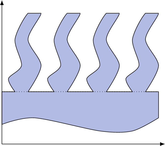
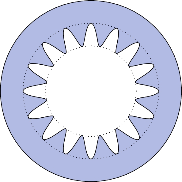
Several critical physical properties of a material are controlled by its geometric construction. Therefore, analyzing the effect of materials geometric structure can help to improve some of its beneficial physical properties and reduce unwanted behavior. This leads to the study of boundary value problems in complex domains such as perforated domain, thin domain, junctions of the thin domain of different configuration (like domain we have considered in this article, with rapidly oscillating boundary), networks, etc. Various constructions shaped as thick junctions or oscillating boundary domains are successfully used in many nano-technologies, micro-techniques, micro-strip radiator, wide-band gap semiconductor, efficient sensor signal processing filters, transistors, heat radiators [17,23,31,32]. This leads to the study of multi-scale analysis and eventually homogenization of boundary value problems in domain with rapidly oscillating boundary. Some sample depictions are given in Figs 1 and 2.

Fig. 1.

Oscillating domain $Ω_{ε}$ .

Fig. 2.

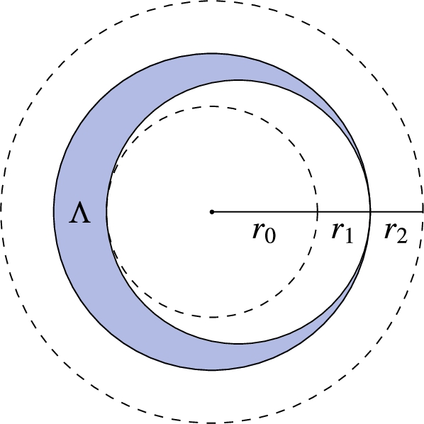
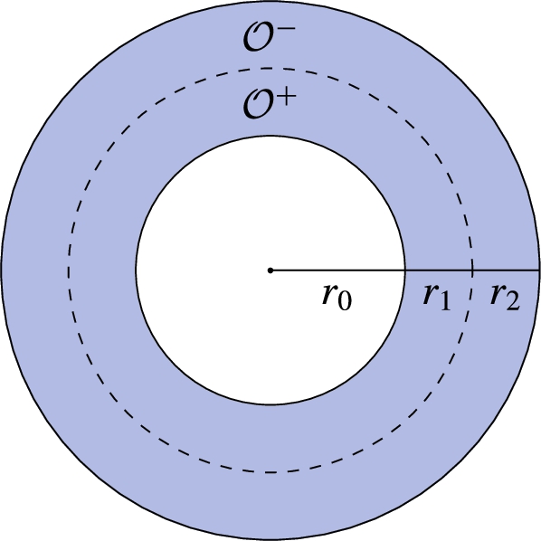
Circular domain $O_{ε}$ .

The study of homogenization on oscillating boundary domain was started by the work done in [30], where the authors have considered Helmholtz equation on oscillating domain to study the limiting behavior of the solution as the oscillating parameter goes to zero. But the proper story begins in 1978 by R. Brizzi and J. P. Chalot in [14], where they have analyzed the asymptotic behavior of Laplace equation with Neumann boundary condition in various oscillating domains as the oscillation parameter vanishes. Subsequently, in this direction, that is, the homogenization of boundary value problems in oscillating domain, a wealthy literature is available. For example, see [1,6,7,10,12,27,28,33,35] and references therein though it is no way exhaustive. The main tools they have used in these articles are asymptotic expansion, extension operators, two-scale convergence, and oscillating test functions. Later, periodic method of unfolding was introduced in [15], and a modified definition of the periodic unfolding method is used in [11] to study homogenization in general oscillating domains and in particular it was quite handy to apply to periodic asymptotic problems including oscillating domains. We remark to mention that most of the article cited so far have pillar type oscillations. Again a large amount of literature is available, but we restrict ourselves to the method of unfolding applied by the present authors and their group. In [2], authors have introduced unfolding operator for the general oscillating domain and as an application they have homogenized a nonlinear elliptic PDE. This unfolding operator and a modified version of this unfolding operator was used to homogenize various boundary value problems and optimal control problems, see, for example [3–5,19,39,40]. Prior to it, unfolding operator is used for the first time to characterize the optimal control, see [37,38].

In all the articles cited above, the source terms were always in $L^{2}$ , so the homogenization procedure happened in a proper Hilbert space set up. In the present work, we consider the source term in $L^{1}$ Banach space and hence we can not expect the solution to be uniformly bounded in $H^{1}$ . To overcome this issue, we will make use of the definition of the renormalized solution, which has been introduced by R. J. DiPerna and P. L. Lions in [20] for the Boltzmann equation. Further, the idea of the renormalized solution has been adapted for the elliptic equation in [8,18]. To see more about the application of renormalized solutions, we refer to the articles [9,13,24,29,34] and references therein.

In the theory of homogenization, the concept of renormalized solution first time used to perform homogenization in [36] by F. Murat. After that, some results though not many, have been reported on homogenization with the renormalized solution. For example, see [21,22,25,26] and references therein. The present work is relatively closer to the work done in [26]. In [26], the authors have considered homogenization of a second-order elliptic PDE in the brush-like or pillar type oscillating domain with source term in $L^{1}$ . As the source term is $L^{1}$ ; the solution has to be understood as a renormalized solution. To get the asymptotic behavior of the renormalized solution, they used the renormalized formulation of the limit problem or homogenized problem corresponding to $L^{2}$ data. Also, compared to the existing articles on homogenization in the oscillating domain, the oscillations are not periodic in [26]. The authors have assumed that the characteristic function of the pillar-base should converge weakly* in $L^{\infty}$ to some strictly positive function. The oscillating test function method was used as a homogenization tool.

In the present article, we consider a second-order elliptic PDE with oscillating coefficients in a general forest type oscillating domain and circular type oscillating domain (see Figs 1 and 2) with source term in $L^{1}$ . This work is a non-trivial generalization of the work done in [26]. In [26], the oscillation is non-periodic, but pillar type; here, we are considering the periodic but very general type of oscillations. We are also allowing the $n - 1$ directional oscillating coefficients in the coefficient matrix. In contrast to [26], extension by ‘zero’ will not be helpful as it will not belong to $H^{1}$ in the non-oscillating direction. To avoid this difficulty, we use the periodic unfolding operator for the general forest oscillating domain (see, [2,16]). In addition, we also consider circular oscillating domain. To carry out the homogenization with $L^{1}$ source term for the circular oscillating domain, first we need to do homogenization for the general second-order elliptic PDE with source term in $L^{2}$ . As it has circular type oscillations, to analyze the asymptotic behavior of the renormalized solution, we have used the periodic unfolding operator in polar coordinates introduced in [2]. Also, we have homogenized the general second-order elliptic PDE with angular oscillations in coefficients, which has not been done in [2].

Let us now explain the organization of the present article and the main ideas of the proofs. In Section 2, we describe the geometry of the domains under consideration. We are considering 2 types of domains namely $Ω_{ε}$ and $O_{ε}$ . The first one $Ω_{ε}$ is the domain with an oscillating boundary, where oscillations are in the horizontal direction. In contrast, the second one $O_{ε}$ has oscillations in the angular direction. The reference cell and limit domain for both cases are also presented. We have included the definition of unfolding operator and its properties for both domains without proof. A detailed explanation is available in [2]. We are also mentioning some auxiliary functions which are important in the study of renormalized solutions.

In Section 3, our aim is to prove the homogenization results of a general second-order PDE in the circular oscillating domain $O_{ε}$ with source term in $L^{1}$ . As it requires the homogenization results with $L^{2}$ data, we are proving it first and then completing the main result. We are using the polar unfolding operator and properties of renormalized solutions to prove our result.

In Section 4, we prove homogenization results of a general second-order PDE in the general oscillating domain $Ω_{ε}$ with source term in $L^{1}$ . Since the proof shows a lot of similarities with the proof we have done in the case of $O_{ε}$ , we are only providing an outline of the proof.

In the Appendix, we are proving the properties of renormalized solutions. We are doing it only for the limit problem of the circular domain. By using the same steps, we can prove similar properties for other renormalized solutions also.

Fig. 3.

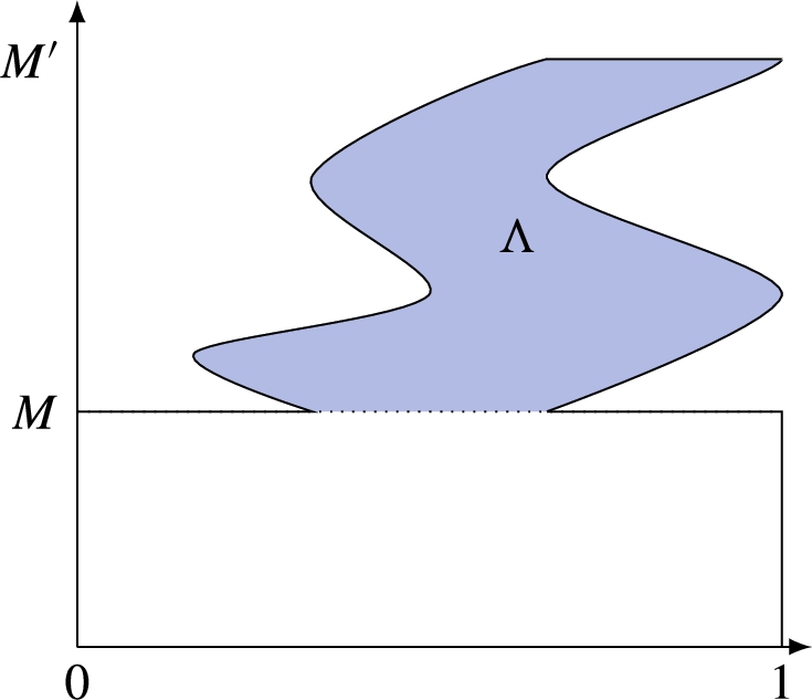
Reference cell Λ.

Fig. 4.

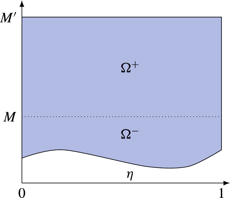
Limit Domain Ω.

2. Domain descriptions, unfolding operators and auxiliary functions

2.1. General oscillating domain $Ω_{ε}$

Let $0 < M < M^{'}$ be real numbers, $Γ_{b} : [0, 1] \to R$ be a Lipschitz continuous function such that $0 < Γ_{b} (x) < M$ and $ε = \frac{1}{n}$ , $n \in N$ . Let Λ be a connected open subset of $Ω^{+} = [0, 1] \times [M, M^{'}]$ with Lipschitz boundary is our reference cell (see Figs 3 and 4). The upper oscillating part of the domain denoted by $Ω_{ε}^{+}$ is given by $\begin{matrix} Ω_{ε}^{+} = {(x_{1}, x_{2}) \in [0, 1] \times [M, M^{'}] : ({\frac{x_{1}}{ε}}, x_{2}) \in Λ}, \end{matrix}$ where $\{\frac{x_{1}}{ε}\}$ denotes the fractional part of $\frac{x_{1}}{ε}$ . The lower fixed part is given by $\begin{matrix} Ω^{-} = {(x_{1}, x_{2}) \in [0, 1] \times [0, M] : Γ_{b} (x_{1}) < x_{2} < M} . \end{matrix}$ The oscillating domain $Ω_{ε} = int (\overline{Ω_{ε}^{+} \cup Ω^{-}})$ and the limit domain $Ω = int (\overline{Ω^{+} \cup Ω^{-}})$ .

For $x_{2} \in (M, M^{'})$ , define the projection of a section in Λ and its measure by $\begin{array}{l} Y (x_{2}) = {y \in [0, 1] : (y, x_{2}) \in Λ}, \\ h (x_{2}) = m (Y (x_{2})), where m denote the Lebesgue measure on R . \end{array}$ This is highly crucial in the definition of the unfolding operators. We assume the following properties on Λ:

The set $Y (x_{2})$ is connected for all $x_{2} \in (M, M^{'})$ ,

There exists $ρ > 0$ such that $0 < ρ ⩽ h (x_{2}) < 1$ for all $x_{2} \in (M, M^{'})$ ,

The boundary part $\partial Λ \cap ([0, 1] \times {x_{2} = M})$ is connected and have positive one dimensional Lebesgue measure.

2.2. Circular oscillating domain $O_{ε}$

Let $0 < r_{0} < r_{1} < r_{2}$ be real numbers, $ε = \frac{1}{n}$ , $n \in N$ . Let Λ be a connected open subset of $R^{2}$ which is contained in the annulus $O^{+} = {(r, θ) : r_{0} < r < r_{1}}$ with Lipschitz boundary is our reference cell (see Figs 5 and 6). Now define $\begin{array}{l} O_{ε}^{+} = {(r, θ) \in O^{+} : (r, {\frac{θ}{ε}}_{2 π}) \in Λ}, O^{-} = {(r, θ) : r_{1} < r < r_{2}}, \\ O_{ε} = int (\overline{O_{ε}^{+} \cup O^{-}}) and O = int (\overline{O^{+} \cup O^{-}}), \end{array}$ where $O_{ε}^{+}$ is the inner oscillating part, $O^{-}$ is the outer fixed part, $O_{ε}$ is the oscillating domain and $O$ is the limit domain. Here ${\{\frac{θ}{ε}\}}_{2 π}$ denotes the fractional part of $\frac{θ}{2 π ε}$ .

For $r \in (r_{0}, r_{1})$ , define $\begin{array}{l} (1) & \begin{matrix} Y (r) = {θ \in [0, 2 π] : (r, θ) \in Λ}, \\ h (r) = \frac{m (Y (r))}{2 π}, where m denotes the Lebesgue measure on R . \end{matrix} \end{array}$ We assume the following properties on Λ:

The set $Y (r)$ is connected for all $r \in (r_{0}, r_{1})$ ,

There exists $ρ > 0$ such that $0 < ρ ⩽ h (r) < 2 π$ for all $r \in (r_{0}, r_{1})$ .

For the sake of completeness, we recall the definition of unfolding operators for

Ω_{ε}

O_{ε}

and its properties without proof. For proof, we refer to [2].

Fig. 5.

Reference cell Λ.

Fig. 6.

Limit Domain $O$ .

Remark 1.

The set of domains that satisfy the hypothesis for rectangular oscillating domains is huge; Fig. 1 is a representative example. Figure 2 is simply a prototype example of the huge collection of circular oscillating domains that satisfy the hypothesis for circular oscillating domains. The analysis for the proofs does not depend on the structure of the domain as long as it satisfies the hypothesis.

2.3. Unfolding operator for

Ω_{ε}

We have already introduced the domain $Ω_{ε}$ with highly oscillating boundary. First, we will define the unfolded domain $Ω_{U}$ in which the unfolded functions are defined. The unfolded domain $Ω_{U}$ is defined as follows: $\begin{matrix} Ω_{U} = {(x_{1}, x_{2}, y) ∣ x_{1} \in (0, 1), x_{2} \in (M, M^{'}), y \in Y (x_{2})} . \end{matrix}$ Let $G = {(x_{2}, y) ∣ x_{2} \in (M, M^{'}), y \in Y (x_{2})}$ , then, one can write, $Ω_{U} = (0, 1) \times G$ . Let $ϕ^{ε} : Ω_{U} \to Ω_{ε}^{+}$ be defined as $ϕ^{ε} (x_{1}, x_{2}, y) = (ε [\frac{x_{1}}{ε}] + ε y, x_{2})$ . The $ε -$ unfolding of a function $u : Ω_{ε}^{+} \to R$ is the function $u \circ ϕ^{ε} : Ω_{U} \to R$ . The operator which maps every function $u : Ω_{ε}^{+} \to R$ to its ε-unfolding is called the unfolding operator. We denote the unfolding operator by $T^{ε}$ , that is, $\begin{matrix} T^{ε} : {u : Ω_{ε}^{+} \to R} \to {T^{ε} (u) : Ω_{U} \to R} \end{matrix}$ is defined by $\begin{matrix} T^{ε} (u) (x_{1}, x_{2}, y) = u (ε [\frac{x_{1}}{ε}] + ε y, x_{2}) . \end{matrix}$ If $U \subset R^{2}$ containing $Ω_{ε}^{+}$ and u is a real valued function on U, $T^{ε} (u)$ means, that is $T^{ε}$ acting on the restriction of u to $Ω_{ε}^{+}$ . Some important properties of the unfolding operator are stated below. For each $ε > 0$ :

$T^{ε}$ is linear. Further, if $u, v : Ω_{ε}^{+} \to R$ , then, $T^{ε} (u v) = T^{ε} (u) T^{ε} (v)$ .

Let $u \in L^{1} (Ω_{ε}^{+})$ . then, $\begin{matrix} \int_{Ω_{U}} T^{ε} (u) = \int_{Ω_{ε}^{+}} u . \end{matrix}$

Let $u \in L^{2} (Ω_{ε}^{+})$ . Then, $T^{ε} u \in L^{2} (Ω_{U})$ and $‖ T^{ε} u ‖_{L^{2} (Ω_{U})} = ‖ u ‖_{L^{2} (Ω_{ε}^{+})}$ .

Let $u \in H^{1} (Ω_{ε}^{+})$ . Then, $T^{ε} u \in L^{2} (0, 1; H^{1} (G))$ . Moreover, $\begin{matrix} \frac{\partial}{\partial x_{2}} T^{ε} u = T^{ε} \frac{\partial u}{\partial x_{2}} and \frac{\partial}{\partial y} T^{ε} u = ε T^{ε} \frac{\partial u}{\partial x_{1}} . \end{matrix}$

Let $u \in L^{2} (Ω_{ε}^{+})$ . Then, $T^{ε} u \to u$ strongly in $L^{2} (Ω_{U})$ . More generally, let $u_{ε} \to u$ strongly in $L^{2} (Ω^{+})$ . Then, $T^{ε} u_{ε} \to u$ strongly in $L^{2} (Ω_{U})$ .

Let, for every ε, $u_{ε} \in L^{2} (Ω_{ε}^{+})$ be such that $T^{ε} u_{ε} ⇀ u$ weakly in $L^{2} (Ω_{U})$ . then, $\begin{matrix} {\tilde{u}}_{ε} ⇀ \int_{Y (x_{2})} u (x_{1}, x_{2}, y) d y weakly in L^{2} (Ω^{+}) . \end{matrix}$

Let, for every $ε > 0$ , $u_{ε} \in H^{1} (Ω_{ε}^{+})$ be such that $T^{ε} u_{ε} ⇀ u$ weakly in $L^{2} (0, 1; H^{1} (G))$ . Then, $\begin{matrix} {\tilde{u}}_{ε} ⇀ \int_{Y (x_{2})} u d y and \tilde{\frac{\partial u_{ε}}{\partial x_{2}}} ⇀ \int_{Y (x_{2})} \frac{\partial u}{\partial x_{2}} d y weakly in L^{2} (Ω^{+}), \end{matrix}$ where ${\tilde{u}}_{ε}$ denotes the extension by 0 of $u_{ε}$ to $Ω^{+}$ . This notation is used through the article.

2.4. Unfolding operator in polar coordinates for $O_{ε}$

Since the oscillations in $O_{ε}$ is in angular direction, we need unfolding operators in polar coordinates to do the analysis. Here we will recall the definition of unfolding operator for $O$ and its properties without proof. For proof one can see [2]. As in the earlier case first, we will define the unfolded domain $O_{U}$ in which the unfolded function are defined. The unfolded domain $O_{U}$ is defined as follows, $\begin{matrix} O_{U} = {(r, θ, τ) ∣ θ \in (0, 2 π), r \in (r_{0}, r_{1}), τ \in Y (r)} . \end{matrix}$ Let $G = {(r, θ, τ) ∣ r \in (r_{0}, r_{1}), θ \in (0, 2 π), τ \in Y (r)}$ , then, we can write, $O_{U} = (0, 2 π) \times G$ . Let $ϕ^{ε} : O_{U} \to O_{ε}^{+}$ be defined as $ϕ^{ε} (θ, r, τ) = (r, ε {[\frac{θ}{ε}]}_{2 π} + ε τ)$ . The ε - unfolding of a function $u : O_{ε}^{+} \to R$ is the function $u \circ ϕ^{ε} : O_{U} \to R$ . The operator which maps every function $u : O_{ε}^{+} \to R$ to its ε-unfolding is called the unfolding operator. Let the unfolding operator be denoted by $T^{ε}$ , that is, $\begin{matrix} T^{ε} : {u : O_{ε}^{+} \to R} \to {T^{ε} (u) : O_{U} \to R} \end{matrix}$ is defined by $\begin{matrix} T^{ε} (u) (r, θ, τ) = u (r, ε {[\frac{θ}{ε}]}_{2 π} + ε τ), \end{matrix}$ where ${[\frac{θ}{ε}]}_{2 π}$ denotes the integer part of $\frac{θ}{2 π ε}$ .

If $U \subset R^{2}$ containing $O_{ε}^{+}$ and u is a real valued function on U, $T^{ε} (u)$ will mean, $T^{ε}$ acting on the restriction of u to $O_{ε}^{+}$ . Some important properties of the circular unfolding operator are stated below. For each $ε > 0$ :

$T^{ε}$ is linear. Further, if $u, v : O_{ε}^{+} \to R$ , then $T^{ε} (u v) = T^{ε} (u) T^{ε} (v)$ .

Let $u \in L^{1} (O_{ε}^{+})$ . then, $\begin{matrix} \int_{O_{U}} T^{ε} (u) = 2 π \int_{O_{ε}^{+}} u . \end{matrix}$

Let $u \in L^{2} (O_{ε}^{+})$ . Then, $T^{ε} u \in L^{2} (O_{U})$ and $‖ T^{ε} u ‖_{L^{2} (O_{U})} = \sqrt{2 π} ‖ u ‖_{L^{2} (O_{ε}^{+})}$ .

Let $u, \frac{\partial u}{\partial r}, \frac{\partial u}{\partial θ} \in L^{2} (O^{+})$ , Then, $T^{ε} u, \frac{\partial}{\partial r} T^{ε} u, \frac{\partial}{\partial τ} T^{ε} u \in L^{2} (O_{U})$ . Moreover, $\begin{matrix} \frac{\partial}{\partial r} T^{ε} u = T^{ε} \frac{\partial u}{\partial r} and \frac{\partial}{\partial τ} T^{ε} u = ε T^{ε} \frac{\partial u}{\partial θ} . \end{matrix}$

Let $u \in L^{2} (O_{ε}^{+})$ . Then, $T^{ε} u \to u$ strongly in $L^{2} (O_{U})$ . More generally, let $u_{ε} \to u$ strongly in $L^{2} (O^{+})$ . Then, $T^{ε} u_{ε} \to u$ strongly in $L^{2} (O_{U})$ .

Let, for every ε, $u_{ε} \in L^{2} (O_{ε}^{+})$ be such that $T^{ε} u_{ε} ⇀ u$ weakly in $L^{2} (O_{U})$ . Then, $\begin{matrix} {\tilde{u}}_{ε} ⇀ \frac{1}{2 π} \int_{Y (r)} u (r, θ, τ) d τ weakly in L^{2} (O^{+}) . \end{matrix}$

Let, for every $ε > 0$ , $u_{ε} \in H^{1} (O_{ε}^{+})$ be such that $T^{ε} u_{ε} ⇀ u$ and $\frac{\partial}{\partial r} T^{ε} u_{ε} ⇀ \frac{\partial u}{\partial r}$ weakly in $L^{2} (O_{U})$ . Then, $\begin{matrix} {\tilde{u}}_{ε} ⇀ \frac{1}{2 π} \int_{Y (r)} u d τ and \tilde{\frac{\partial u_{ε}}{\partial r}} ⇀ \frac{1}{2 π} \int_{Y (r)} \frac{\partial u}{\partial r} d τ weakly in L^{2} (O^{+}), \end{matrix}$ where ${\tilde{u}}_{ε}$ denotes the extension by 0 of $u_{ε}$ to $O^{+}$ .

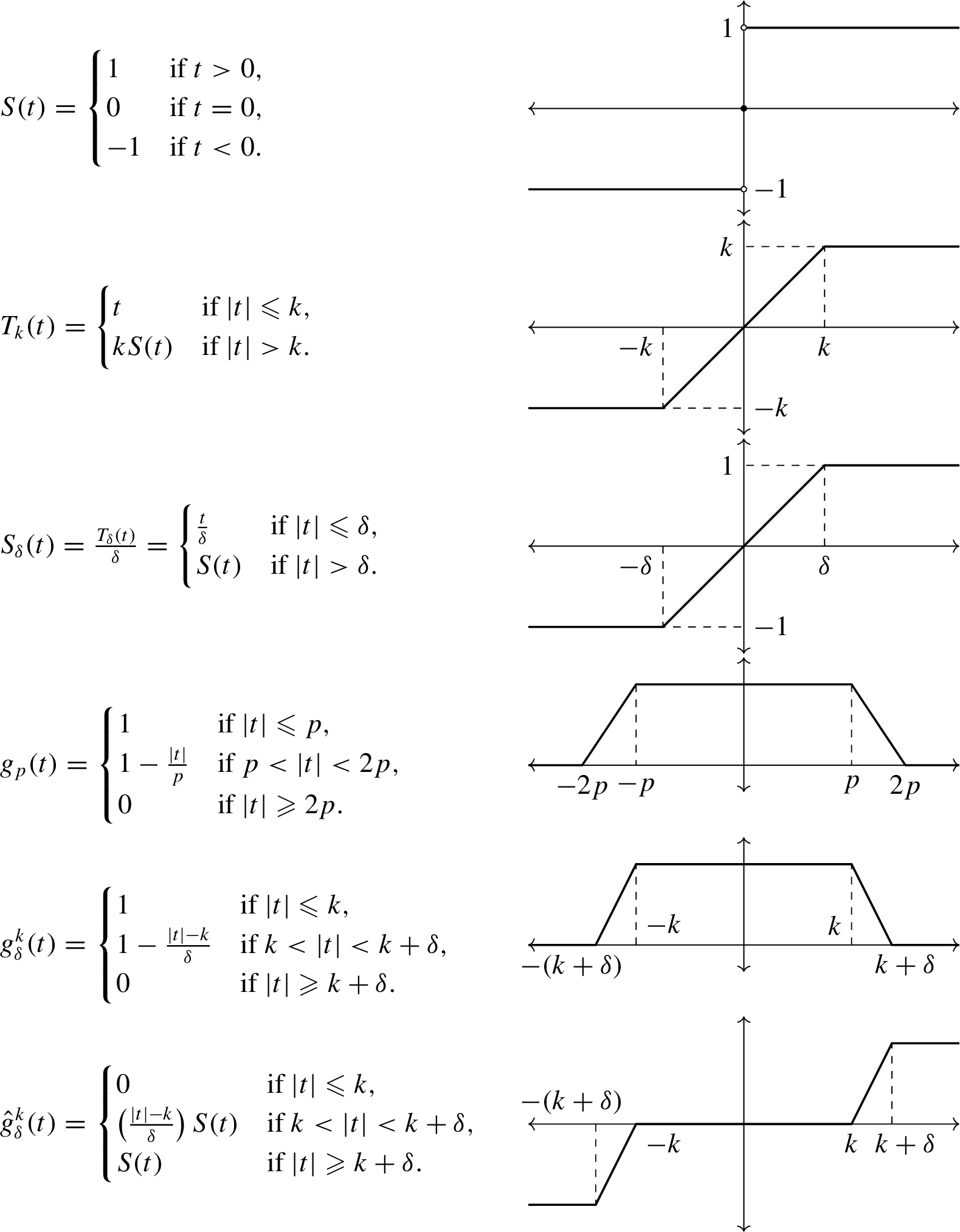
2.5. Auxiliary functions

Here we recall some auxiliary functions which are important in the study of renormalized solutions and homogenization with $L^{1}$ data. The functions defined are standard and available in the literature. For details refer [8,18,26,36]. All the functions are defined from $R \to R$ .

3. Homogenization in $O_{ε}$

To study the asymptotic behavior of elliptic PDE with source term in $L^{1}$ , we need the homogenization results with source term in $L^{2}$ . For the Laplacian it is done in [2], but we need the homogenization results for general second order elliptic PDE in circular domain. So, first we investigate the homogenization results with $L^{2}$ data in $O_{ε}$ . In the whole article, we are not writing the measure while doing integration. It is just for getting the expressions in a simple form. If we are taking the functions in polar coordinates, then the integration is with respect to the measure $r d r d θ$ ; otherwise, it is with respect to the usual Lebesgue Measure. When we are integrating over the unfolded domain, it is better to consider the functions in polar coordinates.

3.1. Homogenization in $O_{ε}$ with $L^{2}$ data

Let $A (r, θ) = {[a_{i, j} (r, θ)]}_{2 \times 2}$ be a $2 \times 2$ matrix where the entries $a_{i j} : O \to R$ are Caratheodory type functions. Also $A (r, θ)$ is uniformly elliptic and bounded in $O$ , that is, there exists $α, β > 0$ such that $\begin{matrix} ⟨ A (x) λ, λ ⟩ ⩾ α | λ |^{2} and | A (x) λ | ⩽ β | λ | \end{matrix}$ for all $λ \in R^{2}$ and a.e. in $O$ . Define $\begin{matrix} A^{ε} (r, θ) = {[a_{i j}^{ε} (r, θ)]}_{2 \times 2} = \{\begin{matrix} A (r, \frac{θ}{ε}) & if (r, θ) \in O^{+}, \\ A (r, θ) & if (r, θ) \in O^{-} . \end{matrix} \end{matrix}$ Consider the following problem in the domain $O_{ε}$ : $\begin{matrix} (2) & \{\begin{matrix} - div (A^{ε} \nabla u_{ε}) + u_{ε} = f & in O_{ε}, \\ A^{ε} \nabla u_{ε} \cdot ν^{ε} = 0 & on \partial O_{ε} . \end{matrix} \end{matrix}$ Here $f \in L^{2} (O)$ is a given function, $ν^{ε}$ is the outward normal vector on $\partial O_{ε}$ . The variational form corresponding to (2) is given as: Find $u_{ε} \in H^{1} (O_{ε})$ such that $\begin{matrix} (3) & \int_{O_{ε}} A^{ε} \nabla u_{ε} \nabla v + u_{ε} v = \int_{O_{ε}} f v for all v \in H^{1} (O_{ε}) . \end{matrix}$ Since the oscillations are in a circular fashion, to study the asymptotic behavior, we need to write the equation in polar form in $O_{ε}^{+}$ as follows: $\begin{matrix} (4) & \int_{O_{ε}^{+}} ([\begin{matrix} α^{ε} & γ^{ε} \\ β^{ε} & η^{ε} \end{matrix}] [\begin{matrix} \frac{\partial u_{ε}}{\partial r} \\ \frac{\partial u_{ε}}{\partial θ} \end{matrix}] [\begin{matrix} \frac{\partial v}{\partial r} \\ \frac{\partial v}{\partial θ} \end{matrix}] + u_{ε} v) + \int_{O^{-}} A \nabla u_{ε} \nabla v + u_{ε} v = \int_{O_{ε}} f v, \end{matrix}$ for all $v \in H^{1} (O_{ε})$ , where $\begin{matrix} (5) & \begin{matrix} α^{ε} = a_{11}^{ε} {cos}^{2} (θ) + a_{12}^{ε} sin (θ) cos (θ) + a_{21}^{ε} sin (θ) cos (θ) + a_{22}^{ε} {sin}^{2} (θ), \\ β^{ε} = \frac{1}{r} (- a_{11}^{ε} sin (θ) cos (θ) - a_{12}^{ε} {sin}^{2} (θ) + a_{21}^{ε} {cos}^{2} (θ) + a_{22}^{ε} sin (θ) cos (θ)), \\ γ^{ε} = \frac{1}{r} (- a_{11}^{ε} sin (θ) cos (θ) + a_{12}^{ε} {cos}^{2} (θ) - a_{21}^{ε} {sin}^{2} (θ) + a_{22}^{ε} sin (θ) cos (θ)) and \\ η^{ε} = \frac{1}{r^{2}} (a_{11}^{ε} {sin}^{2} (θ) - a_{12}^{ε} sin (θ) cos (θ) - a_{21}^{ε} sin (θ) cos (θ) + a_{22}^{ε} {cos}^{2} (θ)) . \end{matrix} \end{matrix}$ Here, we have $α^{ε} = A^{ε} [\begin{matrix} cos (θ) \\ sin (θ) \end{matrix}] [\begin{matrix} cos (θ) \\ sin (θ) \end{matrix}]$ and $det [\begin{matrix} α^{ε} & γ^{ε} \\ β^{ε} & η^{ε} \end{matrix}] = \frac{1}{r^{2}} det A^{ε}$ . Since $A^{ε}$ is coercive, the matrix $[\begin{matrix} α^{ε} & γ^{ε} \\ β^{ε} & η^{ε} \end{matrix}]$ is also coercive.

By definition of unfolding operator (see Section 2.4), we have $T^{ε} (a_{i j}^{ε}) (r, θ, τ) = a_{i j} (r, τ)$ . Since it is independent of ε, for simplicity, we denote $T^{ε} (a_{i j}^{ε})$ as $a_{i j}^{0}$ . Then, from the properties of unfolding operator, we see that $T^{ε} (α^{ε})$ , $T^{ε} (β^{ε})$ , $T^{ε} (γ^{ε})$ and $T^{ε} (η^{ε})$ converges to $α^{0}$ , $β^{0}$ , $γ^{0}$ and $η^{0}$ strongly in $L^{2} (O_{U})$ , respectively, as $ε \to 0$ , where $\begin{matrix} (6) & \begin{matrix} α^{0} = a_{11}^{0} {cos}^{2} (θ) + a_{12}^{0} sin (θ) cos (θ) + a_{21}^{0} sin (θ) cos (θ) + a_{22}^{0} {sin}^{2} (θ), \\ β^{0} = \frac{1}{r} (- a_{11}^{0} sin (θ) cos (θ) - a_{12}^{0} {sin}^{2} (θ) + a_{21}^{0} {cos}^{2} (θ) + a_{22}^{0} sin (θ) cos (θ)), \\ γ^{0} = \frac{1}{r} (- a_{11}^{0} sin (θ) cos (θ) + a_{12}^{0} {cos}^{2} (θ) - a_{21}^{0} {sin}^{2} (θ) + a_{22}^{0} sin (θ) cos (θ)) and \\ η^{0} = \frac{1}{r^{2}} (a_{11}^{0} {sin}^{2} (θ) - a_{12}^{0} sin (θ) cos (θ) - a_{21}^{0} sin (θ) cos (θ) + a_{22}^{0} {cos}^{2} (θ)) . \end{matrix} \end{matrix}$ We want to study the asymptotic behavior of $u_{ε}$ as $ε \to 0$ . First we describe the limit problem.

Limit problem: Consider the Hilbert space $\begin{matrix} V (O) = {ψ \in L^{2} (O) : \frac{\partial ψ}{\partial r} \in L^{2} (O), ψ \in H^{1} (O^{-})}, \end{matrix}$ with the inner product $\begin{matrix} {⟨ ϕ, ψ ⟩}_{V (O)} = {⟨ ϕ, ψ ⟩}_{L^{2} (O^{+})} + {⟨ \frac{\partial ϕ}{\partial r}, \frac{\partial ψ}{\partial r} ⟩}_{L^{2} (O^{+})} + {⟨ ϕ, ψ ⟩}_{H^{1} (O^{-})} . \end{matrix}$ We define the limit problem as follows: Given $f \in L^{2} (O)$ , find $u \in V (O)$ such that $\begin{matrix} (7) & \int_{O^{+}} (a_{0} \frac{\partial u}{\partial r} \frac{\partial v}{\partial r} + h u v) + \int_{O^{-}} (A \nabla u \nabla v + u v) = \int_{O^{+}} h f v + \int_{O^{-}} f v, for all v \in V (O), \end{matrix}$ where $\begin{matrix} a_{0} (r, θ) = \int_{Y (r)} \frac{1}{η^{0}} (α^{0} η^{0} - γ^{0} β^{0}) d τ = \int_{Y (r)} (\frac{det (A (r, τ))}{A (r, τ) [\begin{matrix} - sin (θ) \\ cos (θ) \end{matrix}] [\begin{matrix} - sin (θ) \\ cos (θ) \end{matrix}]}) d τ . \end{matrix}$

Here h and Y are defined as in (1). Since A is elliptic, with elliptic constant α and bounded by β, we have $a_{0} > h (r) \frac{β^{2}}{α}$ . Hence, (7) has a unique solution by Lax–Milgram lemma. We leave the details. We now present the homogenization in circular domain with $L^{2}$ data.

Theorem 1.
Let $u_{ε}$ and u be the unique solutions of ( 4 ) and ( 7 ) respectively. Then, we have the following convergences. $\begin{array}{l} \tilde{u_{ε}} - χ_{O_{ε}} u ⟶ 0 strongly in L^{2} (O), \\ \tilde{\frac{\partial u_{ε}}{\partial r}} - χ_{O_{ε}} \frac{\partial u}{\partial r} ⟶ 0 strongly in L^{2} (O^{+}), \\ \tilde{\frac{\partial u_{ε}}{\partial θ}} - χ_{O_{ε}} (\frac{- β^{ε}}{η^{ε}}) \frac{\partial u}{\partial r} ⟶ 0 strongly in L^{2} (O^{+}), \\ u_{ε} - u ⟶ 0 strongly in H^{1} (O^{-}) . \end{array}$
Proof.
We remark that the second and third convergences are corrector results. By taking $v = u_{ε}$ , in the variational form (3), we get $‖ u_{ε} ‖_{H^{1} (O_{ε})} ⩽ K$ , where K is a generic constant independent of ε. From the integral equality property of unfolding operator, we deduce the following bounds. $\begin{matrix} {‖ T^{ε} u_{ε} ‖}_{L^{2} (O_{U})} ⩽ \sqrt{2 π} ‖ u_{ε} ‖_{L^{2} (O_{ε}^{+})} ⩽ K, {‖ \frac{\partial}{\partial r} T^{ε} u_{ε} ‖}_{L^{2} (O_{U})} ⩽ \sqrt{2 π} {‖ \frac{\partial u_{ε}}{\partial r} ‖}_{L^{2} (O_{ε}^{+})} ⩽ K and \\ {‖ \frac{\partial}{\partial τ} T^{ε} u_{ε} ‖}_{L^{2} (O_{U})} ⩽ ε \sqrt{2 π} {‖ \frac{\partial u_{ε}}{\partial θ} ‖}_{L^{2} (O_{ε}^{+})} ⩽ K . \end{matrix}$ By weak compactness of $L^{2} (O_{U})$ , there exits a sub-sequence (still denoted by ε) and $u^{+} \in L^{2} (O_{U})$ such that $\begin{matrix} (8) & \begin{matrix} T^{ε} u_{ε} ⇀ u^{+} weakly in L^{2} (O_{U}), \\ \frac{\partial}{\partial r} T^{ε} u_{ε} ⇀ \frac{\partial u^{+}}{\partial r}, that is, T^{ε} \frac{\partial u_{ε}}{\partial r} ⇀ \frac{\partial u^{+}}{\partial r} weakly in L^{2} (O_{U}), \\ \frac{\partial}{\partial τ} T^{ε} u_{ε} ⇀ \frac{\partial u^{+}}{\partial τ}, that is, ε T^{ε} \frac{\partial u_{ε}}{\partial θ} ⇀ \frac{\partial u^{+}}{\partial τ} weakly in L^{2} (O_{U}) . \end{matrix} \end{matrix}$ Again since $\{T^{ε} \frac{\partial u_{ε}}{\partial θ}\}$ is bounded in $L^{2} (O_{U})$ , we have $\frac{\partial u}{\partial τ} = 0$ (means $u \in L^{2} (O^{+})$ ) and there exists a $p \in L^{2} (O_{U})$ such that, up-to a sub-sequence, we have $\begin{matrix} (9) & T^{ε} \frac{\partial u_{ε}}{\partial θ} ⇀ p weakly in L^{2} (O_{U}) . \end{matrix}$ Now to identify p, consider $ϕ^{ε} = ε ϕ (r, θ) ψ ({\{\frac{θ}{ε}\}}_{2 π})$ , where $ϕ \in D (O^{+})$ and $ψ \in C^{\infty} [0, 2 π]$ . Then $\begin{matrix} (10) & \begin{matrix} T^{ε} (ϕ^{ε}) = ε T^{ε} (ϕ) ψ (τ), T^{ε} (\frac{\partial ϕ^{ε}}{\partial r}) = ε T^{ε} (\frac{\partial ϕ}{\partial r}) ψ (τ) and \\ T^{ε} (\frac{\partial ϕ^{ε}}{\partial θ}) = ε T^{ε} (\frac{\partial ϕ}{\partial θ}) + T^{ε} (ϕ) ψ^{'} (τ) . \end{matrix} \end{matrix}$

Now use $ϕ^{ε}$ as a test function in (4), we have $\begin{matrix} \int_{O_{ε}^{+}} ([\begin{matrix} α^{ε} & γ^{ε} \\ β^{ε} & η^{ε} \end{matrix}] [\begin{matrix} \frac{\partial u_{ε}}{\partial r} \\ \frac{\partial u_{ε}}{\partial θ} \end{matrix}] [\begin{matrix} \frac{\partial ϕ^{ε}}{\partial r} \\ \frac{\partial ϕ ε}{\partial θ} \end{matrix}] + u_{ε} ϕ^{ε}) = \int_{O_{ε}^{+}} f ϕ^{ε} . \end{matrix}$ Applying unfolding operator, we get $\begin{matrix} \int_{O_{U}} ([\begin{matrix} T^{ε} (α^{ε}) & T^{ε} (γ^{ε}) \\ T^{ε} (β^{ε}) & T^{ε} (η^{ε}) \end{matrix}] [\begin{matrix} T^{ε} \frac{\partial u_{ε}}{\partial r} \\ T^{ε} \frac{\partial u_{ε}}{\partial θ} \end{matrix}] [\begin{matrix} T^{ε} \frac{\partial ϕ^{ε}}{\partial r} \\ T^{ε} \frac{\partial ϕ^{ε}}{\partial θ} \end{matrix}] + T^{ε} (u_{ε}) T^{ε} (ϕ^{ε})) = \int_{O_{U}} T^{ε} (f) T^{ε} (ϕ^{ε}) . \end{matrix}$ Then using (6), (8), (9), (10) and passing to the limit as $ε \to 0$ in the above equation, we obtain $\begin{matrix} \int_{O_{U}} ([\begin{matrix} α^{0} & γ^{0} \\ β^{0} & η^{0} \end{matrix}] [\begin{matrix} \frac{\partial u^{+}}{\partial r} \\ p \end{matrix}] [\begin{matrix} 0 \\ ϕ ψ^{'} \end{matrix}]) = \int_{O_{U}} (β^{0} \frac{\partial u^{+}}{\partial r} + η^{0} p) ϕ (r, θ) ψ^{'} (τ) = 0 . \end{matrix}$ Since $ϕ \in D (O^{+})$ and $ψ \in C^{\infty} [0, 2 π]$ are arbitrary, we have $\begin{matrix} (11) & p = - \frac{β^{0}}{η^{0}} \frac{\partial u^{+}}{\partial r} . \end{matrix}$ Now since in ${u_{ε}}$ is bounded in $H^{1} (O^{-})$ , by weak compactness, there exists $u^{-} \in H^{1} (O^{-})$ such that $\begin{matrix} u_{ε}^{-} ⇀ u^{-} weakly in H^{1} (O^{-}) . \end{matrix}$ Define $\begin{matrix} u (x) = u^{+} χ_{O^{+}} + u^{-} χ_{O^{-}} = \{\begin{matrix} u^{+} (x) & if x \in O^{+}, \\ u^{-} (x) & if x \in O^{-} . \end{matrix} \end{matrix}$
Claim.
$u \in V (O)$ and satisfies the limit problem ( 7 ).

The part that $u \in V (O)$ can be done as in [2] and hence we omit the proof here. Thus, it remains to prove that u satisfies the limit problem (7). Consider $ψ \in C^{\infty} (\overline{O})$ as test a function in (4) to get $\begin{matrix} \int_{O_{ε}^{+}} ([\begin{matrix} α^{ε} & γ^{ε} \\ β^{ε} & η^{ε} \end{matrix}] [\begin{matrix} \frac{\partial u_{ε}}{\partial r} \\ \frac{\partial u_{ε}}{\partial θ} \end{matrix}] [\begin{matrix} \frac{\partial ψ}{\partial r} \\ \frac{\partial ψ}{\partial θ} \end{matrix}] + u_{ε} ψ) + \int_{O^{-}} A \nabla u_{ε} \nabla ψ + u_{ε} ψ = \int_{O_{ε}} f ψ . \end{matrix}$ Applying unfolding, we have $\begin{array}{l} \frac{1}{2 π} \int_{O_{U}} [\begin{matrix} T^{ε} (α^{ε}) & T^{ε} (γ^{ε}) \\ T^{ε} (β^{ε}) & T^{ε} (η^{ε}) \end{matrix}] [\begin{matrix} T^{ε} \frac{\partial u_{ε}}{\partial r} \\ T^{ε} \frac{\partial u_{ε}}{\partial θ} \end{matrix}] [\begin{matrix} T^{ε} \frac{\partial ψ}{\partial r} \\ T^{ε} \frac{\partial ψ}{\partial θ} \end{matrix}] + \frac{1}{2 π} \int_{O_{U}} T^{ε} u_{ε} T^{ε} ψ + \int_{O^{-}} A \nabla u_{ε} \nabla ψ + u_{ε} ψ \\ = \frac{1}{2 π} \int_{O_{U}} T^{ε} f T^{ε} ψ + \int_{O^{-}} f ψ . \end{array}$ Then, using (6), (8) and (9), pass to the limit as $ε \to 0$ in the above equation to obtain $\begin{matrix} \frac{1}{2 π} \int_{O_{U}} ([\begin{matrix} α^{0} & γ^{0} \\ β^{0} & η^{0} \end{matrix}] [\begin{matrix} \frac{\partial u^{+}}{\partial r} \\ p \end{matrix}] [\begin{matrix} \frac{\partial ψ}{\partial r} \\ \frac{\partial ψ}{\partial θ} \end{matrix}] + u^{+} ψ) + \int_{O^{-}} A \nabla u \nabla ψ + u ψ = \frac{1}{2 π} \int_{O_{U}} f ψ + \int_{O^{-}} f ψ . \end{matrix}$ Using the relation (11), the above equation reduces to $\begin{matrix} \frac{1}{2 π} \int_{O_{U}} \frac{1}{η^{0}} (α^{0} η^{0} - γ^{0} β^{0}) \frac{\partial u}{\partial r} \frac{\partial ψ}{\partial r} + u ψ + \int_{O^{-}} A \nabla u \nabla ψ + u ψ = \frac{1}{2 π} \int_{O_{U}} f ψ + \int_{O^{-}} f ψ . \end{matrix}$ Now from the definition of unfolded domain and h, the above equation can be rewritten as $\begin{matrix} \int_{O^{+}} a_{0} \frac{\partial u}{\partial r} \frac{\partial ψ}{\partial r} + h u ψ + \int_{O^{-}} A \nabla u \nabla ψ + u ψ = \int_{O^{+}} h f ψ + \int_{O^{-}} f ψ, \end{matrix}$ where $\begin{matrix} a_{0} (r, θ) = \frac{1}{2 π} \int_{Y (r)} \frac{1}{η^{0}} (α^{0} η^{0} - γ^{0} β^{0}) d τ = \frac{1}{2 π} \int_{Y (r)} (\frac{det (A (r, τ))}{A (r, τ) [\begin{matrix} - sin (θ) \\ cos (θ) \end{matrix}] [\begin{matrix} - sin (θ) \\ cos (θ) \end{matrix}]}) d τ . \end{matrix}$

The last expression can be derived using (6). Hence from the density of $C^{\infty} (\overline{O})$ in $V (O)$ , we see that u satisfies the limit problem (7). Now from (8), (9), (11) and using the properties of unfolding, we have the following convergences: $\begin{array}{l} (12) & \begin{matrix} \tilde{u_{ε}^{+}} ⇀ h u^{+}, \tilde{\frac{\partial u_{ε}^{+}}{\partial r}} ⇀ h \frac{\partial u^{+}}{\partial r}, \\ \tilde{\frac{\partial u_{ε}^{+}}{\partial θ}} ⇀ (- \frac{1}{2 π} \int_{Y (r)} \frac{β^{0}}{η^{0}} d τ) \frac{\partial u^{+}}{\partial r} weakly in L^{2} (O^{+}) and \\ u_{ε}^{-} ⇀ u^{-} weakly in H^{1} (O^{-}) . \end{matrix} \end{array}$ To prove the strong convergences, consider the following energy equality $\begin{matrix} \int_{O_{ε}} A^{ε} \nabla u_{ε} \nabla u_{ε} + u_{ε}^{2} = \int_{O_{ε}} f u_{ε} = \int_{O_{ε}^{+}} f u_{ε} + \int_{O^{-}} f u_{ε} = \frac{1}{2 π} \int_{O_{U}} T^{ε} f T^{ε} u_{ε} + \int_{O^{-}} f u_{ε} . \end{matrix}$ Let us pass to the limit as $ε \to 0$ to get $\begin{array}{l} (13) & \begin{matrix} lim_{ε \to 0} (\int_{O_{ε}} A^{ε} \nabla u_{ε} \nabla u_{ε} + u_{ε}^{2}) & = \int_{O^{+}} h f u + \int_{O^{-}} f u \\ = \int_{O^{+}} a_{0} {(\frac{\partial u}{\partial r})}^{2} + h u^{2} + \int_{O^{-}} A \nabla u \nabla u + u^{2} . \end{matrix} \end{array}$ The last equality follows from the limit problem (7) by taking $v = u$ . To prove the strong convergence, consider the following integral $I^{ε}$ : $\begin{array}{l} I^{ε} = & \int_{O^{+}} [\begin{matrix} α^{ε} & γ^{ε} \\ β^{ε} & η^{ε} \end{matrix}] [\begin{matrix} \tilde{\frac{\partial u_{ε}}{\partial r}} - χ_{O_{ε}} \frac{\partial u}{\partial r} \\ \tilde{\frac{\partial u_{ε}}{\partial θ}} - χ_{O_{ε}} \frac{- β^{ε}}{η^{ε}} \frac{\partial u}{\partial r} \end{matrix}] [\begin{matrix} \tilde{\frac{\partial u_{ε}}{\partial r}} - χ_{O_{ε}} \frac{\partial u}{\partial r} \\ \tilde{\frac{\partial u_{ε}}{\partial θ}} - χ_{O_{ε}} \frac{- β^{ε}}{η^{ε}} \frac{\partial u}{\partial r} \end{matrix}] + \int_{O^{+}} {(\tilde{u_{ε}} - χ_{O_{ε}} u)}^{2} \\ + \int_{O^{-}} A (\nabla u_{ε} - \nabla u) (\nabla u_{ε} - \nabla u) + {(u_{ε} - u)}^{2} . \end{array}$ On expanding, we get $\begin{array}{l} I^{ε} = & \int_{O_{ε}^{+}} [\begin{matrix} α^{ε} & γ^{ε} \\ β^{ε} & η^{ε} \end{matrix}] [\begin{matrix} \frac{\partial u_{ε}}{\partial r} \\ \frac{\partial u_{ε}}{\partial θ} \end{matrix}] [\begin{matrix} \frac{\partial u_{ε}}{\partial r} \\ \frac{\partial u_{ε}}{\partial θ} \end{matrix}] - \int_{O_{ε}^{+}} [\begin{matrix} α^{ε} & γ^{ε} \\ β^{ε} & η^{ε} \end{matrix}] [\begin{matrix} \frac{\partial u_{ε}}{\partial r} \\ \frac{\partial u_{ε}}{\partial θ} \end{matrix}] [\begin{matrix} 1 \\ \frac{- β^{ε}}{η^{ε}} \end{matrix}] \frac{\partial u}{\partial r} \\ - \int_{O_{ε}^{+}} [\begin{matrix} α^{ε} & γ^{ε} \\ β^{ε} & η^{ε} \end{matrix}] [\begin{matrix} 1 \\ \frac{- β^{ε}}{η^{ε}} \end{matrix}] [\begin{matrix} \frac{\partial u_{ε}}{\partial r} \\ \frac{\partial u_{ε}}{\partial θ} \end{matrix}] \frac{\partial u}{\partial r} + \int_{O_{ε}^{+}} [\begin{matrix} α^{ε} & γ^{ε} \\ β^{ε} & η^{ε} \end{matrix}] [\begin{matrix} 1 \\ \frac{- β^{ε}}{η^{ε}} \end{matrix}] [\begin{matrix} 1 \\ \frac{- β^{ε}}{η^{ε}} \end{matrix}] {(\frac{\partial u}{\partial r})}^{2} \\ + \int_{O_{ε}^{+}} ({u_{ε}}^{2} - 2 u_{ε} u + u^{2}) + \int_{O^{-}} (A \nabla u_{ε} \nabla u_{ε} - A \nabla u_{ε} \nabla u - A \nabla u \nabla u_{ε} + A \nabla u \nabla u) \\ + \int_{O^{-}} (u_{ε}^{2} - 2 u_{ε} u + u^{2}) . \end{array}$ On combining first, fifth, eighth and twelfth terms, the above equation can be rewritten as $\begin{array}{l} I^{ε} = & \int_{O_{ε}} (A^{ε} \nabla u_{ε} \nabla u_{ε} + u_{ε}^{2}) - \int_{O_{ε}^{+}} [\begin{matrix} α^{ε} & γ^{ε} \\ β^{ε} & η^{ε} \end{matrix}] [\begin{matrix} \frac{\partial u_{ε}}{\partial r} \\ \frac{\partial u_{ε}}{\partial θ} \end{matrix}] [\begin{matrix} 1 \\ \frac{- β^{ε}}{η^{ε}} \end{matrix}] \frac{\partial u}{\partial r} \\ - \int_{O_{ε}^{+}} [\begin{matrix} α^{ε} & γ^{ε} \\ β^{ε} & η^{ε} \end{matrix}] [\begin{matrix} 1 \\ \frac{- β^{ε}}{η^{ε}} \end{matrix}] [\begin{matrix} \frac{\partial u_{ε}}{\partial r} \\ \frac{\partial u_{ε}}{\partial θ} \end{matrix}] \frac{\partial u}{\partial r} + \int_{O_{ε}^{+}} [\begin{matrix} α^{ε} & γ^{ε} \\ β^{ε} & η^{ε} \end{matrix}] [\begin{matrix} 1 \\ \frac{- β^{ε}}{η^{ε}} \end{matrix}] [\begin{matrix} 1 \\ \frac{- β^{ε}}{η^{ε}} \end{matrix}] {(\frac{\partial u}{\partial r})}^{2} \\ + \int_{O_{ε}^{+}} (- 2 u_{ε} u + u^{2}) + \int_{O^{-}} (- A \nabla u_{ε} \nabla u - A \nabla u \nabla u_{ε} + A \nabla u \nabla u - 2 u_{ε} u + u^{2}) . \end{array}$ Using polar unfolding operator, we arrive at $\begin{array}{l} I^{ε} = & \int_{O_{ε}} (A^{ε} \nabla u_{ε} \nabla u_{ε} + u_{ε}^{2}) - \frac{1}{2 π} \int_{O_{U}} [\begin{matrix} T^{ε} (α^{ε}) & T^{ε} (γ^{ε}) \\ T^{ε} (β^{ε}) & T^{ε} (η^{ε}) \end{matrix}] [\begin{matrix} T^{ε} (\frac{\partial u_{ε}}{\partial r}) \\ T^{ε} (\frac{\partial u_{ε}}{\partial θ}) \end{matrix}] [\begin{matrix} 1 \\ T^{ε} (\frac{- β^{ε}}{η^{ε}}) \end{matrix}] T^{ε} (\frac{\partial u}{\partial r}) \\ - \frac{1}{2 π} \int_{O_{U}} [\begin{matrix} T^{ε} (α^{ε}) & T^{ε} (γ^{ε}) \\ T^{ε} (β^{ε}) & T^{ε} (η^{ε}) \end{matrix}] [\begin{matrix} 1 \\ T^{ε} (\frac{- β^{ε}}{η^{ε}}) \end{matrix}] [\begin{matrix} T^{ε} (\frac{\partial u_{ε}}{\partial r}) \\ T^{ε} (\frac{\partial u_{ε}}{\partial θ}) \end{matrix}] T^{ε} (\frac{\partial u}{\partial r}) \\ + \frac{1}{2 π} \int_{O_{U}} [\begin{matrix} T^{ε} (α^{ε}) & T^{ε} (γ^{ε}) \\ T^{ε} (β^{ε}) & T^{ε} (η^{ε}) \end{matrix}] [\begin{matrix} 1 \\ T^{ε} (\frac{- β^{ε}}{η^{ε}}) \end{matrix}] [\begin{matrix} 1 \\ T^{ε} (\frac{- β^{ε}}{η^{ε}}) \end{matrix}] {(T^{ε} (\frac{\partial u}{\partial r}))}^{2} \\ + \frac{1}{2 π} \int_{O_{U}} (- 2 T^{ε} (u_{ε}) u + T^{ε} (u^{2})) \\ + \int_{O^{-}} (- A \nabla u_{ε} \nabla u - A \nabla u \nabla u_{ε} + A \nabla u \nabla u - 2 u_{ε} u + u^{2}) . \end{array}$ Now using (6), (8), (9), (12) and (13), we get ${lim}_{ε \to 0} I^{ε} = 0$ . Hence, from coercivity of A, we have the strong convergences. This completes the proof. □

We now proceed to establish the homogenization with $L^{1}$ data in circular domain.
3.2. Homogenization in $O_{ε}$ with $L^{1}$ data

With A and $A^{ε}$ is defined as in Section 3.1, consider the following problem: $\begin{matrix} (14) & \{\begin{matrix} - div (A^{ε} \nabla u_{ε}) + u_{ε} = f & in O_{ε}, \\ A^{ε} \nabla u_{ε} \cdot ν^{ε} = 0 & on \partial O_{ε} . \end{matrix} \end{matrix}$

Here, $f \in L^{1} (O)$ is a given function, $ν^{ε}$ is the outward unit normal vector on $\partial O_{ε}$ . As it is well known, we remark that the solution is not defined in the usual weak formulation but using the concept of renormalized solution. Recall the auxiliary function $T_{k}$ defined as in Section 2.5. A function $u_{ε}$ is called a renormalized solution of (14) if $\begin{matrix} (15) & \{\begin{matrix} u_{ε} \in L^{1} (O_{ε}) such that T_{k} (u_{ε}) \in H^{1} (O_{ε}), for all k > 0, \\ \frac{1}{k} ‖ T_{k} (u_{ε}) ‖_{H^{1} (O_{ε})}^{2} \to 0 as k \to \infty, \\ \int_{O_{ε}} A^{ε} \nabla T_{k} (u_{ε}) \nabla (ψ g (u_{ε})) + u_{ε} ψ g (u_{ε}) = \int_{O_{ε}} f ψ g (u_{ε}), \\ for all k > 0, ψ \in H^{1} (O_{ε}) \cap L^{\infty} (O_{ε}), g \in P C_{c}^{1} (R) with supp (g) \subset [- k, k] . \end{matrix} \end{matrix}$

Here $P C_{c}^{1} (R)$ denotes the set of all Lipschitz continuous functions which are piece-wise differentiable on $R$ with compact support. In polar form, we can write (15) as $\begin{matrix} (16) & \{\begin{matrix} u_{ε} \in L^{1} (O_{ε}) such that T_{k} (u_{ε}) \in H^{1} (O_{ε}), for all k > 0, \\ \frac{1}{k} {‖T_{k} (u)‖}_{H^{1} (O_{ε})}^{2} \to 0 as k \to \infty, \\ \int_{O_{ε}^{+}} ([\begin{matrix} α^{ε} & γ^{ε} \\ β^{ε} & η^{ε} \end{matrix}] [\begin{matrix} \frac{\partial}{\partial r} T_{k} (u_{ε}) \\ \frac{\partial}{\partial θ} T_{k} (u_{ε}) \end{matrix}] [\begin{matrix} \frac{\partial}{\partial r} (ψ g (u_{ε})) \\ \frac{\partial}{\partial θ} (ψ g (u_{ε})) \end{matrix}] + T_{k} (u_{ε}) ψ g (u_{ε})) \\ + \int_{O^{-}} A \nabla T_{k} (u_{ε}) \nabla (ψ g (u_{ε})) + T_{k} (u_{ε}) ψ g (u_{ε}) = \int_{O_{ε}} f ψ g (u_{ε}), \\ for all k > 0, ψ \in H^{1} (O_{ε}) \cap L^{\infty} (O_{ε}), g \in P C_{c}^{1} (R) with supp (g) \subset [- k, k] . \end{matrix} \end{matrix}$

We want to study the asymptotic behavior of $u_{ε}$ as $ε \to 0$ . In fact, we prove that the limit problem is the renormalized formulation corresponding to (7).

Limit Problem: We now state the limit problem. Given $f \in L^{1} (O)$ , consider the problem: $\begin{matrix} (17) & \{\begin{matrix} Find u \in L^{1} (O) such that T_{k} (u) \in V (O) for all k > 0, \\ \frac{1}{k} {‖T_{k} (u)‖}_{V (O)}^{2} \to 0 as k \to \infty, \\ \int_{O_{+}} a_{0} \frac{\partial}{\partial r} T_{k} (u) \frac{\partial (ψ g (u))}{\partial r} + h T_{k} (u) ψ g (u) + \int_{O^{-}} A (\nabla T_{k} (u) \nabla (ψ g (u)) + T_{k} (u) ψ g (u)) \\ = \int_{O^{+}} h f ψ g (u) + \int_{O^{-}} f ψ g (u), \\ for all k > 0, ψ \in V (O) \cap L^{\infty} (O), g \in P C_{c}^{1} (R) with supp (g) \subset [- k, k] . \end{matrix} \end{matrix}$

The proof of existence and uniqueness of renormalized solutions of (15), (16), (17) have similar steps. The detailed proof for (17) is done in the Appendix. We now present the homogenization in circular domain with $L^{1}$ data.

Theorem 2.
Let $u_{ε}$ , u be the unique renormalized solutions of ( 16 ) and ( 17 ) respectively. Then, we have the following convergences. $\begin{array}{l} (18) & \tilde{u_{ε}} - χ_{O_{ε}} u ⟶ 0 strongly in L^{1} (O), \\ (19) & \tilde{T_{k} (u_{ε})} - χ_{O_{ε}} T_{k} (u) ⟶ 0 strongly in L^{1} (O) and weakly* in L^{\infty} (O), \\ (20) & \tilde{\frac{\partial}{\partial r} T_{k} (u_{ε})} - χ_{O_{ε}} \frac{\partial}{\partial r} T_{k} (u) ⟶ 0 strongly in L^{2} (O^{+}), \\ (21) & \tilde{\frac{\partial}{\partial θ} T_{k} (u_{ε})} - χ_{O_{ε}} (\frac{- β^{ε}}{η^{ε}}) \frac{\partial}{\partial r} T_{k} (u) ⟶ 0 strongly in L^{2} (O^{+}), \\ (22) & T_{k} (u_{ε}) - T_{k} (u) ⟶ 0 strongly in H^{1} (O^{-}) . \end{array}$
Proof.
We divide the proof into several steps.

Step 1: Proof of (18) and (19). Let $f_{n}$ be a sequence in $L^{2} (O)$ such that $f_{n} \to f$ in $L^{1} (O)$ . Let $u_{ε}^{n}$ , $u^{n}$ be the renormalized solutions of (15) and (17) with source term $f_{n}$ . Then from Theorem 1, for each n, we have $\begin{matrix} \tilde{u_{ε}^{n}} - χ_{O_{ε}} u^{n} ⟶ 0 strongly in L^{2} (O), as ε \to 0 . \end{matrix}$ Now from the Lipschitz property of renormalized solutions (see (64) in the Appendix), we have $\begin{array}{l} ‖ \tilde{u_{ε}} - χ_{O_{ε}} u ‖_{L^{1} (O)} & ⩽ {‖ \tilde{u_{ε}} - \tilde{u_{ε}^{n}} ‖}_{L^{1} (O)} + {‖ \tilde{u_{ε}^{n}} - χ_{O_{ε}} u^{n} ‖}_{L^{1} (O)} + {‖ χ_{O_{ε}} u^{n} - χ_{O_{ε}} u ‖}_{L^{1} (O)} \\ ⩽ 2 ‖ f_{n} - f ‖_{L^{1} (O)} + {‖ \tilde{u_{ε}^{n}} - χ_{O_{ε}} u^{n} ‖}_{L^{1} (O)} . \end{array}$ Thus, we have $\tilde{u_{ε}} - χ_{O_{ε}} \to 0$ strongly in $L^{1} (O_{ε})$ , which is (18). Further, using Lipschitz continuity of $T_{k}$ and Lebesgue Dominated Convergence Theorem, (19) follows.

Step 2: First, we prove weak form of (20), (21) and (22). To get a bound on $T_{k} (u_{ε})$ , we need the energy equality of the equation (15). Energy equality for (17) is proved in the Appendix (see Theorem 5 Step 4). Similar steps can be used to get the following energy equality for (15), $\begin{matrix} \int_{O_{ε}} A^{ε} \nabla T_{k} (u_{ε}) \nabla T_{k} (u_{ε}) + u_{ε} T_{k} (u_{ε}) = \int_{O_{ε}} f T_{k} (u_{ε}) . \end{matrix}$ Since ${(T_{k} (u_{ε}))}^{2} ⩽ u_{ε} T_{k} (u_{ε})$ and A is coercive, we can deduce that $\begin{matrix} \int_{O_{ε}} {| \nabla T_{k} (u_{ε}) |}^{2} + {(T_{k} (u_{ε}))}^{2} = {‖ T_{k} (u_{ε}) ‖}_{H^{1} (O_{ε})}^{2} ⩽ k ‖ f ‖_{L^{1} (O)} . \end{matrix}$ Consider the sequence ${T^{ε} (T_{k} (u_{ε})})$ in $L^{2} (O_{U})$ , where $T^{ε}$ is the unfolding defined as in Section 2.4. From the properties of $T^{ε}$ , we have $\begin{matrix} {‖ T^{ε} (T_{k} (u_{ε})) ‖}_{L^{2} (O_{U})} ⩽ \sqrt{2 π} {‖ T_{k} (u_{ε}) ‖}_{L^{2} (O_{ε}^{+})} ⩽ {(2 π k ‖ f ‖_{L^{1} (O)})}^{\frac{1}{2}}, \\ {‖ \frac{\partial}{\partial r} T^{ε} (T_{k} (u_{ε})) ‖}_{L^{2} (O_{U})} ⩽ \sqrt{2 π} {‖ \frac{\partial}{\partial r} T_{k} (u_{ε}) ‖}_{L^{2} (O_{ε}^{+})} ⩽ {(2 π k ‖ f ‖_{L^{1} (O)})}^{\frac{1}{2}} and \\ {‖ \frac{\partial}{\partial τ} T^{ε} (T_{k} (u_{ε})) ‖}_{L^{2} (O_{U})} ⩽ ε \sqrt{2 π} {‖ \frac{\partial}{\partial θ} T_{k} (u_{ε}) ‖}_{L^{2} (O_{ε}^{+})} ⩽ {(2 π k ‖ f ‖_{L^{1} (O)})}^{\frac{1}{2}} . \end{matrix}$ Hence, by weak compactness, there exists a sub-sequence (still denoted by ε) and $w \in L^{2} (O_{U})$ such that $\begin{matrix} (23) & \begin{matrix} T^{ε} (T_{k} (u_{ε}^{+})) ⇀ w, \frac{\partial}{\partial r} T^{ε} (T_{k} (u_{ε}^{+})) ⇀ \frac{\partial w}{\partial r} and \\ \frac{\partial}{\partial τ} T^{ε} (T_{k} (u_{ε}^{+})) ⇀ \frac{\partial w}{\partial τ} weakly in L^{2} (O_{U}) . \end{matrix} \end{matrix}$ From (19), we get $\begin{matrix} \tilde{T_{k} (u_{ε})} - χ_{O_{ε}} T_{k} (u) ⟶ 0 strongly in L^{2} (O) . \end{matrix}$ Then using the properties of unfolding, we have $\begin{array}{l} T^{ε} (\tilde{T_{k} (u_{ε}^{+})} - χ_{O_{ε}} T_{k} (u^{+})) = T^{ε} (T_{k} (u_{ε}^{+})) - T^{ε} (T_{k} (u^{+})) ⟶ 0 in L^{2} (O_{U}) . \end{array}$ Since $T^{ε} (T_{k} (u^{+})) \to T_{k} (u^{+})$ in $L^{2} (O_{U})$ , it follows that $T^{ε} (T_{k} (u_{ε}^{+})) ⟶ T_{k} (u^{+}) in L^{2} (O_{U})$ . Then from (23), we have $w = T_{k} (u^{+})$ . Thus, we have the following convergences: $\begin{matrix} (24) & \begin{matrix} T^{ε} (T_{k} (u_{ε}^{+})) ⇀ T_{k} (u^{+}) weakly in L^{2} (O_{U}), \\ \frac{\partial}{\partial r} T^{ε} (T_{k} (u_{ε}^{+})) = T^{ε} (\frac{\partial}{\partial r} (T_{k} (u_{ε}^{+}))) ⇀ \frac{\partial}{\partial r} T_{k} (u^{+}) weakly in L^{2} (O_{U}), \\ \frac{\partial}{\partial τ} T^{ε} (T_{k} (u_{ε}^{+})) = ε T^{ε} (\frac{\partial}{\partial θ} (T_{k} (u_{ε}^{+}))) ⇀ \frac{\partial}{\partial τ} T_{k} (u^{+}) = 0 weakly in L^{2} (O_{U}) . \end{matrix} \end{matrix}$ as $u^{+}$ is independent of τ. Now consider the sequence ${T^{ε} (\frac{\partial}{\partial θ} T_{k} (u_{ε}^{+}))}$ which is also bounded in $L^{2} (O_{U})$ and hence will have a weakly convergent sub-sequence. Let $\begin{matrix} (25) & T^{ε} (\frac{\partial}{\partial θ} T_{k} (u_{ε}^{+})) ⇀ p weakly in L^{2} (O_{U}) . \end{matrix}$ Now to evaluate p, consider $ϕ^{ε}$ as in (10) and $g_{δ}^{k}$ as in Section 2.5. Take $v = ϕ^{ε}$ and $g = g_{δ}^{k}$ in (16) to get $\begin{array}{l} \int_{O_{ε}^{+}} A^{ε} \nabla T_{k + 1} (u_{ε}) \nabla ϕ^{ε} g_{δ}^{k} (u_{ε}) + \int_{O_{ε}^{+}} A^{ε} \nabla T_{k + 1} (u_{ε}) \nabla T_{k + 1} (u_{ε}) ϕ^{ε} {(g_{δ}^{k})}^{'} (u_{ε}) \\ + \int_{O_{ε}^{+}} u_{ε} ϕ^{ε} g_{δ}^{k} (u_{ε}) = \int_{O_{ε}^{+}} f ϕ^{ε} g_{δ}^{k} (u_{ε}) . \end{array}$ Now since $g_{δ}^{k} (u_{ε}) \to χ_{{| u_{ε} | ⩽ k}}$ a.e. as $δ \to 0$ , by Lebesgue dominated convergence theorem, as $δ \to 0$ , we obtain: $\begin{array}{l} \int_{O_{ε}} A^{ε} \nabla T_{k + 1} (u_{ε}) \nabla ϕ^{ε} g_{δ}^{k} (u_{ε}) ⟶ \int_{O_{ε}} A^{ε} \nabla T_{k + 1} (u_{ε}) \nabla ϕ^{ε} χ_{{| u_{ε} | ⩽ k}} = \int_{O_{ε}} A^{ε} \nabla T_{k} (u_{ε}) \nabla ϕ^{ε}, \\ \int_{O_{ε}} u_{ε} ϕ^{ε} g_{δ}^{k} (u_{ε}) ⟶ \int_{O_{ε}} u_{ε} ϕ^{ε} χ_{{| u_{ε} | ⩽ k}} and \int_{O_{ε}} f ϕ^{ε} g_{δ}^{k} (u_{ε}) ⟶ \int_{O_{ε}} f ϕ^{ε} χ_{{| u_{ε} | ⩽ k}} . \end{array}$ Therefore, we have $\begin{array}{l} \int_{O_{ε}} A^{ε} \nabla T_{k} (u_{ε}) \nabla ϕ^{ε} + \underset{δ \to 0}{lim sup} \int_{O_{ε}} A^{ε} \nabla T_{k + 1} (u_{ε}) \nabla T_{k + 1} (u_{ε}) ϕ^{ε} {(g_{δ}^{k})}^{'} (u_{ε}) \\ (26) & + \int_{O_{ε}} u_{ε} ϕ^{ε} χ_{{| u_{ε} | ⩽ k}} = \int_{O_{ε}} f ϕ^{ε} χ_{{| u_{ε} | ⩽ k}} . \end{array}$

The last two terms in (26) will converge to 0 as $ε \to 0$ from the definition of $ϕ^{ε}$ . Now, we look into the first two terms. Using polar coordinates and unfolding operator, we can rewrite the first term in the above equation as $\begin{array}{l} \int_{O_{ε}^{+}} A^{ε} \nabla T_{k} (u_{ε}) \nabla ϕ^{ε} & = \int_{O_{ε}^{+}} [\begin{matrix} α^{ε} & γ^{ε} \\ β^{ε} & η^{ε} \end{matrix}] [\begin{matrix} \frac{\partial}{\partial r} T_{k} (u_{ε}) \\ \frac{\partial}{\partial θ} T_{k} (u_{ε}) \end{matrix}] [\begin{matrix} \frac{\partial ϕ^{ε}}{\partial r} \\ \frac{\partial ϕ^{ε}}{\partial θ} \end{matrix}] \\ = \frac{1}{2 π} \int_{O_{U}} [\begin{matrix} T^{ε} (α^{ε}) & T^{ε} (γ^{ε}) \\ T^{ε} (β^{ε}) & T^{ε} (η^{ε}) \end{matrix}] [\begin{matrix} T^{ε} (\frac{\partial}{\partial r} T_{k} (u_{ε})) \\ T^{ε} (\frac{\partial}{\partial θ} T_{k} (u_{ε})) \end{matrix}] [\begin{matrix} T^{ε} \frac{\partial ϕ^{ε}}{\partial r} \\ T^{ε} \frac{\partial ϕ^{ε}}{\partial θ} \end{matrix}] . \end{array}$ Now passing to the limit as $ε \to 0$ using (6), (10), (24) and (25), we get $\begin{array}{l} lim_{ε \to 0} \int_{O_{ε}^{+}} A^{ε} \nabla T_{k} (u_{ε}) \nabla ϕ^{ε} & = \frac{1}{2 π} \int_{O_{U}} [\begin{matrix} α^{0} & γ^{0} \\ β^{0} & η^{0} \end{matrix}] [\begin{matrix} \frac{\partial}{\partial r} T_{k} (u^{+}) \\ p \end{matrix}] [\begin{matrix} 0 \\ ϕ ψ^{'} \end{matrix}] \\ = \frac{1}{2 π} \int_{O_{U}} (β^{0} \frac{\partial}{\partial r} T_{k} (u^{+}) + η^{0} p) ϕ (r, θ) ψ^{'} (τ) . \end{array}$ To handle the second term in (26) let $v = 1$ and $g = {\hat{g}}_{δ}^{k}$ (as defined in Section 2.5) in (16). Here g is not compactly supported, but still we can use it as a test function in (16) due to Theorem 6 in the Appendix. Then $\begin{matrix} \int_{O_{ε}} A^{ε} \nabla T_{k + 1} (u_{ε}) \nabla T_{k + 1} (u_{ε}) {({\hat{g}}_{δ}^{k})}^{'} (u_{ε}) + \int_{O_{ε}} u_{ε} {\hat{g}}_{δ}^{k} (u_{ε}) = \int_{O_{ε}} f {\hat{g}}_{δ}^{k} (u_{ε}) . \end{matrix}$ Since ${({\hat{g}}_{δ}^{k})}^{'} = \frac{1}{δ} χ_{{k ⩽ | u_{ε} | ⩽ k + δ}}$ and $u_{ε} {\hat{g}}_{δ}^{k} (u_{ε}) ⩾ 0$ , we have $\begin{matrix} \frac{1}{δ} \int_{O_{ε}} A^{ε} \nabla T_{k + 1} (u_{ε}) \nabla T_{k + 1} (u_{ε}) χ_{{k ⩽ | u_{ε} | ⩽ k + δ}} ⩽ ‖ f ‖_{L^{1} (O)} . \end{matrix}$ Therefore, we have $\begin{array}{l} \underset{δ \to 0}{lim sup} | \int_{O_{ε}} A^{ε} \nabla T_{k + 1} (u_{ε}) \nabla T_{k + 1} (u_{ε}) ϕ^{ε} {(g_{δ}^{k})}^{'} (u_{ε}) | \\ ⩽ ε \underset{δ \to 0}{lim sup} \frac{1}{δ} \int_{O_{ε}} A^{ε} \nabla T_{k + 1} (u_{ε}) \nabla T_{k + 1} (u_{ε}) χ_{{k ⩽ | u_{ε} | ⩽ k + δ}} ⩽ ε ‖ f ‖_{L^{1} (O)}, \end{array}$ which implies $\begin{matrix} (27) & \underset{ε \to 0}{lim sup} (\underset{δ \to 0}{lim sup} \int_{O_{ε}} A^{ε} \nabla T_{k + 1} (u_{ε}) \nabla T_{k + 1} (u_{ε}) ϕ^{ε} {(g_{δ}^{k})}^{'} (u_{ε})) = 0 . \end{matrix}$ Hence passing to the limit as $ε \to 0$ in (26) we get $\begin{matrix} \int_{O_{U}} (β^{0} \frac{\partial}{\partial r} T_{k} (u^{+}) + η^{0} p) ϕ (r, θ) ψ^{'} (τ) = 0 . \end{matrix}$ Since $ϕ \in D (O^{+})$ and $ψ \in C^{\infty} [0, 2 π]$ are arbitrary, we have $\begin{matrix} (28) & p = - \frac{β^{0}}{η^{0}} \frac{\partial}{\partial r} T_{k} (u^{+}) . \end{matrix}$ Then, using (24) and properties of unfolding, we have $\begin{matrix} (29) & \begin{matrix} \tilde{T_{k} (u_{ε}^{+})} ⇀ h T_{k} (u^{+}), \tilde{\frac{\partial}{\partial r} T_{k} (u_{ε}^{+})} ⇀ h \frac{\partial}{\partial r} T_{k} (u^{+}) and \\ \tilde{\frac{\partial}{\partial θ} T_{k} (u_{ε}^{+})} ⇀ (- \frac{1}{2 π} \int_{Y (r)} \frac{β^{0}}{η^{0}} d τ) \frac{\partial}{\partial r} T_{k} (u^{+}) weakly in L^{2} (O^{+}) . \end{matrix} \end{matrix}$ Since $‖ T_{k} (u_{ε}) ‖_{H^{1} (O^{-})} ⩽ {(k ‖ f ‖_{L^{1} (O)})}^{\frac{1}{2}}$ , from weak compactness, we have up-to a sub-sequence $\begin{matrix} (30) & T_{k} (u_{ε}) ⇀ v weakly in H^{1} (O^{-}) \end{matrix}$ as $ε \to 0$ . Thus, from (19), we have $v = T_{k} (u^{-})$ .

Step 3: Now, we prove the strong convergences in (20), (21) and (22). Using the energy equality for renormalized formulations of (15) and (17), we have the following energy convergence $\begin{array}{l} lim_{ε \to 0} \int_{O_{ε}} A^{ε} \nabla T_{k} (u_{ε}) \nabla T_{k} (u_{ε}) + u_{ε} T_{k} (u_{ε}) \\ = lim_{ε \to 0} \int_{O_{ε}} f T_{k} (u_{ε}) = lim_{ε \to 0} \int_{O^{+}} f \tilde{T_{k} (u_{ε})} + \int_{O^{-}} f T_{k} (u_{ε}) = \int_{O^{+}} h f T_{k} (u^{+}) + \int_{O^{-}} f T_{k} (u^{-}) \\ (31) & = \int_{O^{+}} a_{0} {(\frac{\partial}{\partial r} T_{k} (u))}^{2} + h u T_{k} (u) + \int_{O^{-}} A \nabla T_{k} (u) \nabla T_{k} (u) + u T_{k} (u) . \end{array}$ On the other hand, we have $\begin{array}{l} \int_{O_{ε}} u_{ε} T_{k} (u_{ε}) = & \int_{O^{+}} ({\tilde{u}}_{ε} - χ_{O_{ε}} u) \tilde{T_{k} (u_{ε})} + \int_{O^{+}} u (\tilde{T_{k} (u_{ε})} - χ_{O_{ε}} T_{k} (u)) \\ (32) & + \int_{O^{+}} u χ_{O_{ε}} T_{k} (u) + \int_{O^{-}} u_{ε} T_{k} (u_{ε}) . \end{array}$ Now passing to the limit as $ε \to 0$ in (32) using (18) and (19), we get $\begin{matrix} (33) & lim_{ε \to 0} \int_{O_{ε}} u_{ε} T_{k} (u_{ε}) = \int_{O^{+}} h u T_{k} (u) + \int_{O^{-}} u T_{k} (u) . \end{matrix}$ Combining (31) and (33), we have $\begin{matrix} (34) & lim_{ε \to 0} \int_{O_{ε}} A^{ε} \nabla T_{k} (u_{ε}) \nabla T_{k} (u_{ε}) = \int_{O^{+}} a_{0} {(\frac{\partial}{\partial r} T_{k} (u))}^{2} + \int_{O^{-}} A \nabla T_{k} (u) \nabla T_{k} (u) . \end{matrix}$ Now consider the following integral $I^{ε}$ and we need to prove $I^{ε} \to 0$ . $\begin{array}{l} I^{ε} = & \int_{O^{+}} [\begin{matrix} α^{ε} & γ^{ε} \\ β^{ε} & η^{ε} \end{matrix}] [\begin{matrix} \tilde{\frac{\partial}{\partial r} T_{k} (u_{ε})} - χ_{O_{ε}} \frac{\partial}{\partial r} T_{k} (u) \\ \tilde{\frac{\partial}{\partial θ} T_{k} (u_{ε})} - χ_{O_{ε}} (\frac{- β^{ε}}{η^{ε}}) \frac{\partial}{\partial r} T_{k} (u) \end{matrix}] [\begin{matrix} \tilde{\frac{\partial}{\partial r} T_{k} (u_{ε})} - χ_{O_{ε}} \frac{\partial}{\partial r} T_{k} (u) \\ \tilde{\frac{\partial}{\partial θ} T_{k} (u_{ε})} - χ_{O_{ε}} (\frac{- β^{ε}}{η^{ε}}) \frac{\partial}{\partial r} T_{k} (u) \end{matrix}] \\ + \int_{O^{-}} A (\nabla T_{k} (u_{ε}) - \nabla T_{k} (u)) (\nabla T_{k} (u_{ε}) - \nabla T_{k} (u)) . \end{array}$ On expanding, we get $\begin{array}{rcl} I^{ε} & = & \int_{O_{ε}^{+}} [\begin{matrix} α^{ε} & γ^{ε} \\ β^{ε} & η^{ε} \end{matrix}] [\begin{matrix} \frac{\partial}{\partial r} T_{k} (u_{ε}) \\ \frac{\partial}{\partial θ} T_{k} (u_{ε}) \end{matrix}] [\begin{matrix} \frac{\partial}{\partial r} T_{k} (u_{ε}) \\ \frac{\partial}{\partial θ} T_{k} (u_{ε}) \end{matrix}] - \int_{O_{ε}^{+}} [\begin{matrix} α^{ε} & γ^{ε} \\ β^{ε} & η^{ε} \end{matrix}] [\begin{matrix} \frac{\partial}{\partial r} T_{k} (u_{ε}) \\ \frac{\partial}{\partial θ} T_{k} (u_{ε}) \end{matrix}] [\begin{matrix} 1 \\ \frac{- β^{ε}}{η^{ε}} \end{matrix}] \frac{\partial}{\partial r} T_{k} (u) \\ - \int_{O_{ε}^{+}} [\begin{matrix} α^{ε} & γ^{ε} \\ β^{ε} & η^{ε} \end{matrix}] [\begin{matrix} 1 \\ \frac{- β^{ε}}{η^{ε}} \end{matrix}] [\begin{matrix} \frac{\partial}{\partial r} T_{k} (u_{ε}) \\ \frac{\partial}{\partial θ} T_{k} (u_{ε}) \end{matrix}] \frac{\partial}{\partial r} T_{k} (u) + \int_{O_{ε}^{+}} [\begin{matrix} α^{ε} & γ^{ε} \\ β^{ε} & η^{ε} \end{matrix}] [\begin{matrix} 1 \\ \frac{- β^{ε}}{η^{ε}} \end{matrix}] [\begin{matrix} 1 \\ \frac{- β^{ε}}{η^{ε}} \end{matrix}] {(\frac{\partial}{\partial r} T_{k} (u))}^{2} \\ + \int_{O^{-}} (A \nabla T_{k} (u_{ε}) \nabla T_{k} (u_{ε}) - A \nabla T_{k} (u_{ε}) \nabla T_{k} (u) - A \nabla T_{k} (u) \nabla T_{k} (u_{ε}) + A \nabla T_{k} (u) \nabla T_{k} (u)) . \end{array}$ Combine first and fifth terms to get $\begin{array}{rcl} I^{ε} & = & \int_{O_{ε}} (A^{ε} \nabla T_{k} (u_{ε}) \nabla T_{k} (u_{ε}) + T_{k} {(u_{ε})}^{2}) - \int_{O_{ε}^{+}} [\begin{matrix} α^{ε} & γ^{ε} \\ β^{ε} & η^{ε} \end{matrix}] [\begin{matrix} \frac{\partial}{\partial r} T_{k} (u_{ε}) \\ \frac{\partial}{\partial θ} T_{k} (u_{ε}) \end{matrix}] [\begin{matrix} 1 \\ \frac{- β^{ε}}{η^{ε}} \end{matrix}] \frac{\partial}{\partial r} T_{k} (u) \\ - \int_{O_{ε}^{+}} [\begin{matrix} α^{ε} & γ^{ε} \\ β^{ε} & η^{ε} \end{matrix}] [\begin{matrix} 1 \\ \frac{- β^{ε}}{η^{ε}} \end{matrix}] [\begin{matrix} \frac{\partial}{\partial r} T_{k} (u_{ε}) \\ \frac{\partial}{\partial θ} T_{k} (u_{ε}) \end{matrix}] \frac{\partial}{\partial r} T_{k} (u) + \int_{O_{ε}^{+}} [\begin{matrix} α^{ε} & γ^{ε} \\ β^{ε} & η^{ε} \end{matrix}] [\begin{matrix} 1 \\ \frac{- β^{ε}}{η^{ε}} \end{matrix}] [\begin{matrix} 1 \\ \frac{- β^{ε}}{η^{ε}} \end{matrix}] {(\frac{\partial}{\partial r} T_{k} (u))}^{2} \\ + \int_{O^{-}} (- A \nabla T_{k} (u_{ε}) \nabla T_{k} (u) - A \nabla T_{k} (u) \nabla T_{k} (u_{ε}) + A \nabla T_{k} (u) \nabla T_{k} (u)) . \end{array}$ Using polar unfolding operator, we arrive at $\begin{array}{l} I^{ε} = & \int_{O_{ε}} A^{ε} \nabla T_{k} (u_{ε}) \nabla T_{k} (u_{ε}) \\ - \frac{1}{2 π} \int_{O_{U}} [\begin{matrix} T^{ε} (α^{ε}) & T^{ε} (γ^{ε}) \\ T^{ε} (β^{ε}) & T^{ε} (η^{ε}) \end{matrix}] [\begin{matrix} T^{ε} (\frac{\partial}{\partial r} T_{k} (u_{ε})) \\ T^{ε} (\frac{\partial}{\partial θ} T_{k} (u_{ε})) \end{matrix}] [\begin{matrix} 1 \\ T^{ε} (\frac{- β^{ε}}{η^{ε}}) \end{matrix}] T^{ε} (\frac{\partial}{\partial r} T_{k} (u)) \\ - \frac{1}{2 π} \int_{O_{U}} [\begin{matrix} T^{ε} (α^{ε}) & T^{ε} (γ^{ε}) \\ T^{ε} (β^{ε}) & T^{ε} (η^{ε}) \end{matrix}] [\begin{matrix} 1 \\ T^{ε} (\frac{- β^{ε}}{η^{ε}}) \end{matrix}] [\begin{matrix} T^{ε} (\frac{\partial}{\partial r} T_{k} (u_{ε})) \\ T^{ε} (\frac{\partial}{\partial θ} T_{k} (u_{ε})) \end{matrix}] T^{ε} (\frac{\partial}{\partial r} T_{k} (u)) \\ + \frac{1}{2 π} \int_{O_{U}} [\begin{matrix} T^{ε} (α^{ε}) & T^{ε} (γ^{ε}) \\ T^{ε} (β^{ε}) & T^{ε} (η^{ε}) \end{matrix}] [\begin{matrix} 1 \\ T^{ε} (\frac{- β^{ε}}{η^{ε}}) \end{matrix}] [\begin{matrix} 1 \\ T^{ε} (\frac{- β^{ε}}{η^{ε}}) \end{matrix}] {(T^{ε} (\frac{\partial}{\partial r} T_{k} (u)))}^{2} \\ + \int_{O^{-}} (- A \nabla T_{k} (u_{ε}) \nabla T_{k} (u) - A \nabla T_{k} (u) \nabla T_{k} (u_{ε}) + A \nabla T_{k} (u) \nabla T_{k} (u)) . \end{array}$ Now using (6), (24), (25), (28) and (34), we get ${lim}_{ε \to 0} I^{ε} = 0$ . Then, by coercivity of A, we have (20), (21) and (22). □
Remark 2.
In the above problem, we did not put oscillation on the coefficient in the fixed part $O^{-}$ to avoid extra calculations. In the fixed domain with oscillating coefficient and $L^{1}$ source term, the homogenization results are straightforward from the existing literature on homogenization with $L^{1}$ data, for example, see [22].
Remark 3.
Here we considered the circular oscillating domain only in 2-dimension due to the complexity in modeling circular oscillations in higher dimensions. We are working on it and hope that we will do it in the future.

4. Homogenization in $Ω_{ε}$

The aim of this section is to study the homogenization of a general oscillating elliptic operator with $L^{1}$ data in the very general oscillating domain $Ω_{ε}$ (see Fig. 1). For this purpose, first, we need the homogenization results with $L^{2}$ data which are available in the literature (refer [2] and [39]). But to move on to $L^{1}$ data, we need the strong convergence results which are not there in the literature. So, first we will see some strong convergence result in general forest type oscillating domain with source term f in $L^{2}$ . Since the aim of the article is to do homogenization with $L^{1}$ data on domains with boundary having general oscillations, we are doing analysis only in 2 dimension to make the presentation simpler. It can be extended to $n -$ dimensional domain with $n - 1$ directional oscillation with minor modification which we done already with $L^{2}$ data in [39].

4.1. Homogenization in $Ω^{ε}$ with $L^{2}$ data

Let $A (x_{1}, x_{2}) = {[a_{i, j} (x_{1}, x_{2})]}_{2 \times 2}$ be a $2 \times 2$ matrix, where the entries $a_{i j} : Ω \to R$ are Caratheodory type functions, 1-periodic in $x_{1}$ direction. Also $A (x_{1}, x_{2})$ is uniformly elliptic and bounded in Ω, that is, there exists $α, β > 0$ such that $\begin{matrix} ⟨ A (x) λ, λ ⟩ ⩾ α | λ |^{2} and | A (x) λ | ⩽ β | λ | \end{matrix}$ for all $λ \in R^{2}$ and a.e. in Ω. Define $\begin{matrix} A^{ε} (x_{1}, x_{2}) = \{\begin{matrix} A (\frac{x_{1}}{ε}, x_{2}) & if (x_{1}, x_{2}) \in Ω^{+}, \\ A (x_{1}, x_{2}) & if (x_{1}, x_{2}) \in Ω^{-} . \end{matrix} \end{matrix}$

Note.
Here for simplicity we only consider 2 variable case. The same steps will work for n variable.

Consider the following problem in the domain $Ω_{ε}$ : $\begin{matrix} \{\begin{matrix} - div (A^{ε} \nabla u_{ε}) + u_{ε} = f & in Ω_{ε}, \\ A^{ε} \nabla u_{ε} \cdot ν^{ε} = 0 & on \partial Ω_{ε} . \end{matrix} \end{matrix}$ Here $f \in L^{2} (Ω)$ is a given function, $ν^{ε}$ is the outward unit normal vector. Corresponding variational formulation is $\begin{matrix} (35) & \{\begin{matrix} Find u \in H^{1} (Ω_{ε}) such that \\ \int_{Ω_{ε}} A^{ε} \nabla u_{ε} \nabla v + u_{ε} v = \int_{Ω^{ε}} f v, for all v \in H^{1} (Ω_{ε}) . \end{matrix} \end{matrix}$ We want to study the asymptotic behavior of $u_{ε}$ as $ε \to 0$ . Let us look at the limit problem.

Limit problem: Consider the Hilbert space $\begin{matrix} W (Ω) = {ψ \in L^{2} (Ω) : \frac{\partial ψ}{\partial x_{2}} \in L^{2} (Ω), ψ |_{Ω^{-}} \in H^{1} (Ω^{-})} \end{matrix}$ with inner product $\begin{matrix} {⟨ ϕ, ψ ⟩}_{W (Ω)} = {⟨ ϕ, ψ ⟩}_{L^{2} (Ω^{+})} + {⟨ \frac{\partial ϕ}{\partial x_{2}}, \frac{\partial ψ}{\partial x_{2}} ⟩}_{L^{2} (Ω^{+})} + {⟨ ϕ, ψ ⟩}_{H^{1} (Ω^{-})} . \end{matrix}$ We define the limit problem as follows: Given $f \in L^{2} (Ω)$ , find $u \in W (Ω)$ such that $\begin{matrix} (36) & \int_{Ω^{+}} a_{0} \frac{\partial u}{\partial x_{2}} \frac{\partial ψ}{\partial x_{2}} + h u ψ + \int_{Ω^{-}} A \nabla u \nabla ψ + u ψ = \int_{Ω^{+}} h f ψ + \int_{Ω^{-}} f ψ for all ψ \in W (Ω), \end{matrix}$ where $\begin{matrix} a_{0} (x_{1}, x_{2}) = a_{0} (x_{2}) = \int_{Y (x_{2})} \frac{det (A (y, x_{2}))}{a_{11} (y, x_{2})} d y . \end{matrix}$
Theorem 3.
Let $u_{ε}$ , u be the unique solutions of ( 35 ) and ( 36 ) respectively. Then, we have the following convergences $\begin{array}{l} (37) & \begin{matrix} \tilde{u_{ε}} - χ_{Ω_{ε}} u ⟶ 0 strongly in L^{2} (Ω), \\ \tilde{\frac{\partial u_{ε}}{\partial x_{2}}} - χ_{Ω_{ε}} \frac{\partial u}{\partial x_{2}} ⟶ 0 strongly in L^{2} (Ω^{+}), \\ \frac{\partial u_{ε}}{\partial x_{1}} - χ_{Ω_{ε}} (\frac{- a_{12}^{ε}}{a_{11}^{ε}}) \frac{\partial u}{\partial x_{2}} ⟶ 0 strongly in L^{2} (Ω^{+}), \\ u_{ε} - u ⟶ 0 strongly in H^{1} (Ω^{-}) . \end{matrix} \end{array}$

Proof of Theorem 3 is similar to that of Theorem 1. So we are giving only an outline of the proof.
Proof.
Since $‖ u_{ε} ‖_{H^{1} (Ω_{ε})} ⩽ ‖ f ‖_{L^{2} (Ω)}$ , using the properties of unfolding operator defined in Section 2.3 we have ${T^{ε} (u_{ε})}$ is bounded in $L^{2} ((0, 1); H^{1} (G))$ and hence from weak compactness, there exist $u^{+}, p \in L^{2} (Ω_{U})$ such that $\begin{matrix} (38) & \begin{matrix} T^{ε} u_{ε} ⇀ u^{+}, T^{ε} \frac{\partial u_{ε}}{\partial x_{2}} ⇀ \frac{\partial u^{+}}{\partial x_{2}}, T^{ε} \frac{\partial u_{ε}}{\partial x_{1}} ⇀ p and \\ ε T^{ε} \frac{\partial u_{ε}}{\partial x_{1}} ⇀ \frac{\partial u^{+}}{\partial x_{2}} = 0 weakly in L^{2} (Ω_{U}) . \end{matrix} \end{matrix}$ For $ϕ \in D (Ω^{+})$ and $ψ \in C^{\infty} ([0, 1])$ , define $ϕ^{ε} = ε ϕ (x) ψ ({\frac{x_{1}}{ε}})$ . Then $\begin{matrix} (39) & \begin{matrix} T^{ε} (ϕ^{ε}) = ε T^{ε} (ϕ) ψ (y), \frac{\partial}{\partial x_{2}} T^{ε} (ϕ^{ε}) = ε T^{ε} (\frac{\partial ϕ}{\partial x_{2}}) ψ (y) and \\ T^{ε} (\frac{\partial ϕ^{ε}}{\partial x_{1}}) = ε T^{ε} (\frac{\partial ϕ}{\partial x_{1}}) + T^{ε} (ϕ) ψ^{'} (y) . \end{matrix} \end{matrix}$ Using $ϕ^{ε}$ as a test function in (35), apply unfolding operator and passing to the limit using (38) and (39) to get $\begin{matrix} p (x_{1}, x_{2}, y) = - \frac{a_{12} (y, x_{2})}{a_{11} (y, x_{2})} \frac{\partial u^{+}}{\partial x_{2}} (x_{1}, x_{2}) . \end{matrix}$ Again since $‖ u_{ε} ‖_{H^{1} (Ω_{ε})} ⩽ ‖ f ‖_{L^{2} (Ω)}$ , there exists a $u^{-} \in H^{1} (Ω^{-})$ such that $\begin{matrix} u_{ε} \to u^{-} weakly in Ω^{-} . \end{matrix}$ Define $u = χ_{Ω^{+}} u^{+} + χ_{Ω^{-}} u^{-}$ . From ([2], Theorem 4.1), we have $u \in W (Ω)$ . Now use $ψ \in C^{\infty} (Ω)$ as test function in (35). Apply unfolding operator and passing to the limit using (38), we obtain $\begin{array}{l} \int_{Ω_{U}} [\begin{matrix} a_{11} (y, x_{2}) & a_{12} (y, x_{2}) \\ a_{21} (y, x_{2}) & a_{22} (y, x_{2}) \end{matrix}] [\begin{matrix} - \frac{a_{12} (y, x_{2})}{a_{11} (y, x_{2})} \frac{\partial u}{\partial x_{2}} \\ 1 \end{matrix}] [\begin{matrix} \frac{\partial ψ}{\partial x_{1}} \\ \frac{\partial ψ}{\partial x_{2}} \end{matrix}] + u ψ + \int_{Ω^{-}} A \nabla u \nabla ψ + u ψ \\ = \int_{Ω_{U}} f ψ + \int_{Ω^{-}} f ψ . \end{array}$ On simplifying, deduce that $\begin{array}{l} \int_{Ω^{+}} a_{0} \frac{\partial u}{\partial x_{2}} \frac{\partial ψ}{\partial x_{2}} + h u ψ + \int_{Ω^{-}} A \nabla u \nabla ψ + u ψ = \int_{Ω^{+}} h f ψ + \int_{Ω^{-}} f ψ, \\ where a_{0} (x_{1}, x_{2}) = a_{0} (x_{2}) = \int_{Y (x_{2})} \frac{det (A (y, x_{2}))}{a_{11} (y, x_{2})} d y . \end{array}$ By density of $C^{\infty} (Ω)$ in $W (Ω)$ we get that u satisfies the limit problem (36). Using $u_{ε}$ as a test function in (35) and passing to the limit as $ε \to 0$ , we get the following energy convergence: $\begin{matrix} (40) & lim_{ε \to 0} (\int_{Ω_{ε}} A^{ε} \nabla u_{ε} \nabla u_{ε} + u_{ε}^{2}) = \int_{Ω^{+}} a_{0} {(\frac{\partial u}{\partial x_{2}})}^{2} + h u^{2} + \int_{Ω^{-}} A \nabla u \nabla u + u^{2} . \end{matrix}$ Now to prove the strong convergence, consider the following integral $\begin{array}{l} I^{ε} = & \int_{Ω^{+}} A^{ε} (\tilde{\nabla u_{ε}} - χ_{Ω_{ε}} \frac{\partial}{\partial x_{2}} u [\begin{matrix} - \frac{a_{12}^{ε}}{a_{11}^{ε}} \\ 1 \end{matrix}]) (\tilde{\nabla u_{ε}} - χ_{Ω_{ε}} \frac{\partial}{\partial x_{2}} u [\begin{matrix} - \frac{a_{12}^{ε}}{a_{11}^{ε}} \\ 1 \end{matrix}]) \\ + \int_{Ω^{+}} {(\tilde{u_{ε}} - χ_{Ω_{ε}} u)}^{2} + \int_{Ω^{-}} A (\nabla u_{ε} - \nabla u) (\nabla u_{ε} - \nabla u) + \int_{Ω^{-}} {(u_{ε} - u)}^{2} . \end{array}$ As we have done in Theorem 1, expand the expression, apply unfolding operator and passing to the limit using (38) and (40), we get ${lim}_{ε \to 0} I^{ε} = 0$ . Hence the coercevity of A implies the result. □

We now consider the homogenization in $Ω_{ε}$ with $f \in L^{1} (Ω)$ .
4.2. Homogenization in $Ω^{ε}$ with $L^{1}$ data

With A and $A^{ε}$ as in Section 4.1, consider the following problem in the domain $Ω_{ε}$ : $\begin{matrix} (41) & \{\begin{matrix} - div (A^{ε} \nabla u_{ε}) + u_{ε} = f & in Ω_{ε}, \\ A^{ε} \nabla u_{ε} \cdot ν^{ε} = 0 & on \partial Ω_{ε} . \end{matrix} \end{matrix}$ Here $f \in L^{1} (Ω)$ is a given function, $ν^{ε}$ is the outward normal vector on $\partial Ω_{ε}$ . A function $u_{ε}$ is a renormalized solution of (41) if $\begin{matrix} (42) & \{\begin{matrix} u_{ε} \in L^{1} (Ω_{ε}) such that T_{k} (u_{ε}) \in H^{1} (Ω_{ε}), for all k > 0, \\ \frac{1}{k} {‖T_{k} (u)‖}_{H^{1} (Ω_{ε})}^{2} \to 0, as k \to \infty, \\ \int_{Ω_{ε}} A^{ε} \nabla T_{k} (u_{ε}) \nabla (v g (u_{ε})) + u_{ε} v g (u_{ε}) = \int_{Ω_{ε}} f v g (u_{ε}), \\ for all k > 0, v \in H^{1} (Ω_{ε}) \cap L^{\infty} (Ω_{ε}), g \in P C_{c}^{1} (R) with supp (g) \subset [- k, k] . \end{matrix} \end{matrix}$ We wish to study the asymptotic behavior of $u_{ε}$ as $ε \to 0$ . As we have done in the circular case, the limit problem is nothing but the renormalized formulation of (36). Again, we only sketch the proof here.

Limit problem: Given $f \in L^{1} (Ω)$ , consider the following problem: $\begin{matrix} (43) & \{\begin{matrix} Find u \in L^{1} (Ω) such that T_{k} (u) \in W (Ω), for all k > 0, \\ \frac{1}{k} {‖T_{k} (u)‖}_{W (Ω)}^{2} \to 0 as k \to \infty, \\ \int_{Ω^{+}} a_{0} \frac{\partial T_{k} (u)}{\partial x_{2}} \frac{\partial (ψ g (u))}{\partial x_{2}} + h u ψ g (u) + \int_{Ω^{-}} A \nabla T_{k} (u) \nabla (ψ g (u)) + u ψ g (u) \\ = \int_{Ω^{+}} h f ψ g (u) + \int_{Ω^{-}} f ψ g (u), \\ for all k > 0, ψ \in W (Ω) \cap L^{\infty} (Ω), g \in P C_{c}^{1} (R) with supp (g) \subset [- k, k] . \end{matrix} \end{matrix}$ The proof for existence and uniqueness of renormalized solutions of (42) and (43) are analogous to the proof for (17) which is done in the Appendix.

Theorem 4.

Let $u_{ε}$ , u be the unique renormalized solutions of ( 42 ) and ( 43 ) respectively. Then, we have the following convergences $\begin{array}{l} (44) & \tilde{u_{ε}} - χ_{Ω_{ε}} u ⟶ 0 strongly in L^{1} (Ω), \\ (45) & \tilde{T_{k} (u_{ε})} - χ_{Ω_{ε}} T_{k} (u) ⟶ 0 strongly in L^{1} (Ω) and weakly* in L^{\infty} (Ω), \\ (46) & \tilde{\frac{\partial}{\partial x_{2}} T_{k} (u_{ε})} - χ_{Ω_{ε}} \frac{\partial}{\partial x_{2}} T_{k} (u) ⟶ 0 strongly in L^{2} (Ω^{+}), \\ (47) & \tilde{\frac{\partial}{\partial x_{1}} T_{k} (u_{ε})} - χ_{Ω_{ε}} (- \frac{a_{12}^{ε}}{a_{11}^{ε}}) \frac{\partial}{\partial x_{2}} T_{k} (u) ⟶ 0 strongly in L^{2} (Ω^{+}), \\ (48) & T_{k} (u_{ε}) - T_{k} (u) ⟶ 0 strongly in H^{1} (Ω^{-}) . \end{array}$

Proof.

The convergences (44) and (45) can be proved using the same steps as those in step 1 of Theorem 2. That is using Lipschitz property of renormalized solutions and homogenization results with $L^{2}$ data. Now using the energy equality of (42), we get $‖ T_{k} (u_{ε}) ‖_{H^{1} (Ω_{ε})}^{2} ⩽ k ‖ f ‖_{L^{1} Ω^{ε}}$ . Hence from the properties of unfolding operator, there exists a $w \in L^{2} ((0, 1); H^{1} (G))$ and $p \in L^{2} (Ω_{U})$ such that $\begin{matrix} (49) & \begin{matrix} T^{ε} (T_{k} (u_{ε}^{+})) ⇀ w weakly in L^{2} ((0, 1); H^{1} (G)) and \\ T^{ε} (\frac{\partial}{\partial x_{1}} T_{k} (u_{ε})) ⇀ p weakly in L^{2} (Ω_{U}) . \end{matrix} \end{matrix}$ Now from (45), using the properties of unfolding, we have $\begin{matrix} T^{ε} (\tilde{T_{k} (u_{ε}^{+})} - χ_{Ω_{ε}} T_{k} (u^{+})) = T^{ε} (T_{k} (u_{ε}^{+})) - T^{ε} (T_{k} (u^{+})) ⟶ 0 in L^{2} (Ω_{U}) . \end{matrix}$ Since $T^{ε} (T_{k} (u^{+})) ⟶ (T_{k} (u^{+}))$ in $L^{2} (Ω_{U})$ , we get $w = T_{k} (u^{+})$ . In (42), let $v = ϕ^{ε}$ as defined in (39) and $g = g_{δ}^{k}$ and follow the same steps as we have done in the proof of Theorem 2 to obtain $\begin{array}{l} \int_{Ω_{ε}} A^{ε} \nabla T_{k + 1} (u_{ε}) \nabla ϕ^{ε} g_{δ}^{k} (u_{ε}) + \int_{Ω_{ε}} A^{ε} \nabla T_{k + 1} (u_{ε}) \nabla T_{k + 1} (u_{ε}) ϕ^{ε} {(g_{δ}^{k})}^{'} (u_{ε}) \\ + \int_{Ω_{ε}} u_{ε} ϕ^{ε} g_{δ}^{k} (u_{ε}) = \int_{Ω_{ε}} f ϕ^{ε} g_{δ}^{k} (u_{ε}) . \end{array}$ Since $g_{δ}^{k} (u_{ε}) \to χ_{{| u_{ε} | ⩽ k}}$ a.e. as $δ \to 0$ , by Lebesgue dominated convergence theorem, as $δ \to 0$ , we deduce that $\begin{array}{l} \int_{Ω_{ε}} A^{ε} \nabla T_{k + 1} (u_{ε}) \nabla ϕ^{ε} + \underset{δ \to 0}{lim sup} \int_{Ω_{ε}} A^{ε} \nabla T_{k + 1} (u_{ε}) \nabla T_{k + 1} (u_{ε}) ϕ^{ε} {g_{δ}^{k}}^{'} (u_{ε}) \\ + \int_{Ω_{ε}} u_{ε} ϕ^{ε} χ_{{| u_{ε} | ⩽ k}} = \int_{Ω_{ε}} f ϕ^{ε} χ_{{| u_{ε} | ⩽ k}} . \end{array}$ Apply unfolding operator on the first term and passing to the limit as $ε \to 0$ to get $\begin{array}{l} (50) & \int_{Ω_{U}} [\begin{matrix} a_{11} (y, x_{2}) & a_{12} (y, x_{2}) \\ a_{21} (y, x_{2}) & a_{22} (y, x_{2}) \end{matrix}] [\begin{matrix} p \\ \frac{\partial}{\partial x_{2}} T_{k} (u) \end{matrix}] [\begin{matrix} ϕ (x) ψ^{'} (y) \\ 0 \end{matrix}] \\ + \underset{ε \to 0}{lim sup} (\underset{δ \to 0}{lim sup} \int_{Ω_{ε}} A^{ε} \nabla T_{k + 1} (u_{ε}) \nabla T_{k + 1} (u_{ε}) ϕ^{ε} {g_{δ}^{k}}^{'} (u_{ε})) = 0 . \end{array}$ By using the same steps as we done to obtain (27), we can get $\begin{matrix} \underset{ε \to 0}{lim sup} (\underset{δ \to 0}{lim sup} \int_{Ω_{ε}} A^{ε} \nabla T_{k + 1} (u_{ε}) \nabla T_{k + 1} (u_{ε}) ϕ^{ε} {(g_{δ}^{k})}^{'} (u_{ε})) = 0 . \end{matrix}$ Hence from (50), we have $\begin{array}{l} \int_{Ω_{U}} [\begin{matrix} a_{11} (y, x_{2}) & a_{12} (y, x_{2}) \\ a_{21} (y, x_{2}) & a_{22} (y, x_{2}) \end{matrix}] [\begin{matrix} p \\ \frac{\partial}{\partial x_{2}} T_{k} (u) \end{matrix}] [\begin{matrix} ϕ (x) ψ^{'} (y) \\ 0 \end{matrix}] \\ = \int_{Ω_{U}} (a_{11} p + a_{12} \frac{\partial}{\partial x_{2}} T_{k} (u)) ϕ (x_{1}, x_{2}) ψ^{'} (y) = 0 . \end{array}$ Since the above equality is true for all $ϕ \in D (Ω^{+})$ and $ψ \in C^{\infty} [0, 1]$ , we have $\begin{matrix} p = - \frac{a_{12}}{a_{11}} \frac{\partial}{\partial x_{2}} T_{k} (u) . \end{matrix}$ Since ${T_{k} (u_{ε}^{-})}$ is bounded in $H^{1} (Ω^{-})$ , from weak compactness, we have up-to a sub-sequence $\begin{matrix} (51) & T_{K} (u_{ε}) ⇀ v weakly in H^{1} (Ω^{-}) . \end{matrix}$ Then from (44), we have $v = T_{k} (u^{-})$ .

We now prove the corresponding strong convergences (corrector results). Using the energy equality for renormalized formulations of (42) and (43), we have the following energy convergence $\begin{array}{l} \int_{Ω_{ε}} A^{ε} \nabla T_{k} (u_{ε}) \nabla T_{k} (u_{ε}) + u_{ε} T_{k} (u_{ε}) ⟶ & \int_{Ω^{+}} a_{0} {(\frac{\partial T_{k} (u)}{\partial x_{2}})}^{2} + h u T_{k} (u) \\ + \int_{Ω^{-}} A \nabla T_{k} (u) \nabla T_{k} (u) + u T_{k} (u) . \end{array}$ As we have done in Step 3 of proof of Theorem 2, using the above convergence we can deduce that $\begin{matrix} (52) & lim_{ε \to 0} \int_{Ω_{ε}} A^{ε} \nabla T_{k} (u_{ε}) \nabla T_{k} (u_{ε}) = \int_{Ω^{+}} a_{0} {(\frac{\partial T_{k} (u)}{\partial x_{2}})}^{2} + \int_{Ω^{-}} A \nabla T_{k} (u) \nabla T_{k} (u) . \end{matrix}$ To get the strong convergence results consider the following integral $\begin{array}{l} I^{ε} = & \int_{Ω^{+}} A^{ε} (\tilde{\nabla T_{k} (u_{ε})} - χ_{Ω_{ε}} \frac{\partial}{\partial x_{2}} T_{k} (u) [\begin{matrix} - \frac{a_{12}^{ε}}{a_{11}^{ε}} \\ 1 \end{matrix}]) (\tilde{\nabla T_{k} (u_{ε})} - χ_{Ω_{ε}} \frac{\partial}{\partial x_{2}} T_{k} (u) [\begin{matrix} - \frac{a_{12}^{ε}}{a_{11}^{ε}} \\ 1 \end{matrix}]) \\ + \int_{Ω^{-}} A (\nabla T_{k} (u_{ε}) - \nabla T_{k} (u)) (\nabla T_{k} (u_{ε}) - \nabla T_{k} (u)) . \end{array}$

Now expand $I^{ε}$ and apply unfolding operator. Then passing to the limit as $ε \to 0$ using (49), (51) and (52) to get ${lim}_{ε \to 0} I^{ε} = 0$ . From coercivity property of A, we get the corrector result (46), (47) and (48). This completes the proof of the theorem. □

Remark 4.

Here, we considered $Ω_{ε} \in R^{2}$ , to make the presentation simpler. All the results still hold and the proofs are similar if $Ω_{ε} \subset R^{n}$ , for any finite n.

Footnotes

Acknowledgements

We wish to express our appreciation to the referees for their fruitful comments and suggestions in the first version of the paper, which helped us to improve our article’s quality. The first and third authors would like to thank the Department of Mathematics, IISc, Bangalore, India, and the second author would like to thank TIFR Center for Applicable Mathematics, Bangalore, India, for the academic support. The third author would like to acknowledge the National Board for Higher Mathematics (NBHM), Department of Atomic Energy(DAE), India, for the financial support. The first author would also like to thank Department of Science and Technology (DST), Government of India for the partial financial support under Project No. CRG/2021/000458.

Renormalized solutions

In the Appendix, we prove the existence, uniqueness and Lipschitz property of renormalized solutions. We will prove it only for the circular limit system (17). The result will follow along the same steps for the other limit system (43).

From (7), for $ψ \in V (O), (u_{n} - u_{m})$ satisfies $\begin{array}{l} \int_{O^{+}} a_{0} \frac{\partial (u_{n} - u_{m})}{\partial r} \frac{\partial ψ}{\partial r} + h (u_{n} - u_{m}) ψ + \int_{O^{-}} A \nabla (u_{n} - u_{m}) \nabla ψ + (u_{n} - u_{m}) ψ \\ = \int_{O^{+}} h (f_{n} - f_{m}) ψ + \int_{O^{-}} (f_{n} - f_{m}) ψ . \end{array}$ Now from the definition of $S_{δ} = \frac{T_{δ}}{δ}$ , we have $S_{δ} (u_{n} - u_{m}) \in V (O)$ . Choosing $ψ = S_{δ} (u_{n} - u_{m})$ as a test function in the above variational form, we get $\begin{array}{l} \int_{O^{+}} \frac{1}{δ} a_{0} {(\frac{\partial}{\partial r} T_{δ} (u_{n} - u_{m}))}^{2} + h (u_{n} - u_{m}) S_{δ} (u_{n} - u_{m}), \\ + \int_{O^{-}} \frac{1}{δ} A \nabla T_{δ} (u_{n} - u_{m}) \nabla T_{δ} (u_{n} - u_{m}) + (u_{n} - u_{m}) S_{δ} (u_{n} - u_{m}), \\ = \int_{O^{+}} h (f_{n} - f_{m}) S_{δ} (u_{n} - u_{m}) + \int_{O^{-}} (f_{n} - f_{m}) S_{δ} (u_{n} - u_{m}) . \end{array}$ Now $S_{δ} \to S$ as $δ \to 0$ point-wise, applying Lebesgue dominated convergence theorem, and ellipticity of $a_{0}$ and A, we get $\begin{matrix} \int_{O^{+}} h (u_{n} - u_{m}) S (u_{n} - u_{m}) + \int_{O^{-}} (u_{n} - u_{m}) S (u_{n} - u_{m}) ⩽ ‖ f_{n} - f_{m} ‖_{L^{1} (O)} \end{matrix}$ which implies $‖ u_{n} - u_{m} ‖_{L^{1} (O)} ⩽ ‖ f_{n} - f_{m} ‖_{L^{1} (O)}$ . Hence ${u_{n}}$ is Cauchy and hence convergent to some u in $L^{1} (O)$ .

Step 2: Now, we will show that for each k, an $n \to \infty$ $\begin{array}{l} (53) & T_{k} (u_{n}) \to T_{k} (u) strongly in L^{1} (O) and weakly* in L^{\infty} (O), \\ (54) & T_{k} (u_{n}) ⇀ T_{k} (u) weakly in V (O) . \end{array}$ The convergence (53) follows from the strong convergence of $u_{n} \to u$ in $L^{1}$ and the fact that $T_{k}$ is a bounded Lipschitz continuous function. Let us now prove (54). Choosing $T_{k} (u_{n})$ as a test function in (7), we get $\begin{array}{l} \int_{O^{+}} a_{0} {(\frac{\partial T_{k} (u_{n})}{\partial r})}^{2} + h u_{n} T_{k} (u_{n}) + \int_{O^{-}} A \nabla T_{k} (u_{n}) \nabla T_{k} (u_{n}) + u_{n} T_{k} (u_{n}) \\ (55) & = \int_{O^{+}} h f_{n} T_{k} (u_{n}) + \int_{O^{-}} f_{n} T_{k} (u_{n}) . \end{array}$ The definition of $T_{k}$ implies that $t T_{k} (t) ⩾ | T_{k} (t) |^{2}$ . Thus, from the ellipticity of $a_{0}$ and A, it follows that $\begin{array}{l} \int_{O^{+}} {| \frac{\partial T_{k} (u_{n})}{\partial r} |}^{2} + \int_{O^{+}} {| T_{k} (u_{n}) |}^{2} + \int_{O^{-}} {| \nabla T_{k} (u_{n}) |}^{2} + \int_{O^{-}} {| T_{k} (u_{n}) |}^{2} \\ (56) & ⩽ k ‖ f_{n} ‖_{L^{1} (O)} ⩽ k sup_{n} ‖ f_{n} ‖_{L^{1} (O)} . \end{array}$

Hence, for each k, ${T_{k} (u_{n})}$ is a bounded sequence in the Hilbert space $V (O)$ and hence have a sub-sequence converges weakly. But we already have $T_{k} (u_{n}) \to T_{k} (u)$ in $L^{2} (O)$ which gives us (54).

Step 3: We claim that $\frac{1}{k} ‖ T_{k} (u) ‖_{V (O)}^{2} \to 0$ as $k \to \infty$ . From (55), we have $\begin{matrix} \frac{1}{k} {‖ T_{k} (u_{n}) ‖}_{V (O)}^{2} ⩽ \int_{O} f_{n} \frac{T_{k} (u_{n})}{k} . \end{matrix}$ Thus, we have $\begin{matrix} \underset{n}{lim sup} (\frac{1}{k} {‖ T_{k} (u_{n}) ‖}_{V (O)}^{2}) ⩽ \int_{O} f \frac{T_{k} (u)}{k} . \end{matrix}$ Using the fact that $\frac{T_{k} (t)}{k} \to 0$ for every t, applying Lebesgue dominated convergence theorem to the right hand side and pass to limit as $k \to \infty$ , we see that $\begin{matrix} (57) & \underset{n}{lim sup} (\frac{1}{k} {‖ T_{k} (u_{n}) ‖}_{V (O)}^{2}) \to 0 as k \to \infty . \end{matrix}$ Then, from weak lower semi-continuity of norm in Hilbert Space, we have the desired result.

Step 4: In this step, we will show that the limit satisfies the following energy equality. $\begin{array}{l} \int_{O^{+}} a_{0} {(\frac{\partial}{\partial r} T_{k} (u))}^{2} + h u T_{k} (u) + \int_{O^{-}} A \nabla T_{k} (u) \nabla T_{k} (u) + u T_{k} (u) \\ (58) & = \int_{O^{+}} h f T_{k} (u) + \int_{O^{-}} f T_{k} (u) . \end{array}$ Throughout this step $k > 0$ is fixed. Let $g_{p}$ be defined as in Section 2.5. Consider $T_{k} (u) g_{p} (u_{n})$ as a test function in (7) with $f = f_{n}$ and $u = u_{n}$ to get $\begin{array}{l} \int_{O^{+}} a_{0} ({(\frac{\partial u_{n}}{\partial r})}^{2} T_{k} (u) g_{p}^{'} (u_{n}) + \frac{\partial u_{n}}{\partial r} \frac{\partial}{\partial r} T_{k} (u) g_{p} (u_{n})) + h u_{n} T_{k} (u) g_{p} (u_{n}) \\ + \int_{O^{-}} A (\nabla u_{n} \nabla u_{n} T_{k} (u) g_{p}^{'} (u_{n}) + \nabla u_{n} \nabla T_{k} (u) g_{p} (u_{n})) + u_{n} T_{k} (u) g_{p} (u_{n}) \\ (59) & = \int_{O^{+}} h f T_{k} (u) g_{p} (u_{n}) + \int_{O^{-}} f T_{k} (u) g_{p} (u_{n}) . \end{array}$ We now fix $p > k$ , then as $n \to \infty$ , we have from (53) and (54) that $\begin{array}{l} \int_{O^{+}} a_{0} \frac{\partial u_{n}}{\partial r} \frac{\partial}{\partial r} T_{k} (u) g_{p} (u_{n}) + h u_{n} T_{k} (u) g_{p} (u_{n}) \\ = \int_{O^{+}} a_{0} \frac{\partial T_{2 p} (u_{n})}{\partial r} \frac{\partial}{\partial r} T_{k} (u) g_{p} (u_{n}) + h u T_{k} (u) g_{p} (u_{n}) \\ ⟶ \int_{O^{+}} a_{0} \frac{\partial T_{2 p} (u)}{\partial r} \frac{\partial}{\partial r} T_{k} (u) g_{p} (u) + h u T_{k} (u) g_{p} (u), \\ \int_{O^{-}} A \nabla u_{n} \nabla T_{k} (u) g_{p} (u_{n}) + u_{n} T_{k} (u) g_{p} (u_{n}) ⟶ \int_{O^{-}} A \nabla T_{2 p} (u) \nabla T_{k} (u) g_{p} (u) + u T_{k} (u) g_{p} (u), \\ \int_{O^{+}} h f T_{k} (u) g_{p} (u_{n}) + \int_{O^{-}} f T_{k} (u) g_{p} (u_{n}) ⟶ \int_{O^{+}} h f T_{k} (u) g_{p} (u) + \int_{O^{-}} f T_{k} (u) g_{p} (u) . \end{array}$ Since ${lim}_{p \to \infty} g_{p} (x) \to 1$ , we have $\begin{array}{l} \int_{O^{+}} a_{0} \frac{\partial T_{2 p} (u)}{\partial r} \frac{\partial}{\partial r} T_{k} (u) g_{p} (u) + h u T_{k} (u) g_{p} (u) ⟶ \int_{O^{+}} a_{0} {(\frac{\partial}{\partial r} T_{k} (u))}^{2} + h u T_{k} (u), \\ \int_{O^{-}} A \nabla T_{2 p} (u) \nabla T_{k} (u) g_{p} (u) + u_{n} T_{k} (u) g_{p} (u) ⟶ \int_{O^{-}} A \nabla T_{k} (u) \nabla T_{k} (u) + u T_{k} (u), \\ \int_{O^{+}} h f T_{k} (u) g_{p} (u) + \int_{O^{-}} f T_{k} (u) g_{p} (u) ⟶ \int_{O^{+}} h f T_{k} (u) + \int_{O^{-}} f T_{k} (u) . \end{array}$ Now coming to the remaining terms in (59), we get $\begin{array}{l} \underset{n}{lim sup} | \int_{O^{+}} a_{0} {(\frac{\partial u_{n}}{\partial r})}^{2} T_{k} (u) g_{p}^{'} (u_{n}) + \int_{O^{-}} A \nabla u_{n} \nabla u_{n} T_{k} (u) g_{p}^{'} (u_{n}) | \\ ⩽ 2 k \underset{n}{lim sup} \frac{1}{2 p} (\int_{O^{+}} a_{0} {(\frac{\partial T_{2 p} (u_{n})}{\partial r})}^{2} + \int_{O^{-}} A \nabla T_{2 p} (u_{n}) \nabla T_{2 p} (u_{n})) \\ ⩽ 2 k \underset{n}{lim sup} (\frac{1}{2 p} ‖ T_{2 p} ‖_{V (O)}^{2}) \to 0 as p \to \infty . (Using (57)) \end{array}$ So by letting n and then p to infinity in (59), we get the energy estimate (58).

Step 5: Here, we will prove the following strong convergence: $\begin{matrix} (60) & T_{k} (u_{n}) \to T_{k} (u) strongly in V (O) . \end{matrix}$ Using the energy equality (58), we have as $n \to \infty$ , $\begin{array}{l} (61) & \begin{matrix} lim_{n \to \infty} \int_{O^{+}} a_{0} {(\frac{\partial T_{k} (u_{n})}{\partial r})}^{2} + h u_{n} T_{k} (u_{n}) + \int_{O^{-}} A \nabla T_{k} (u_{n}) \nabla T_{k} (u_{n}) + u_{n} T_{k} (u_{n}) \\ = lim_{n \to \infty} \int_{O^{+}} h f T_{k} (u_{n}) + \int_{O^{-}} f T_{k} (u_{n}) \\ = \int_{O^{+}} h f T_{k} (u) + \int_{O^{-}} f T_{k} (u) \\ = \int_{O^{+}} a_{0} {(\frac{\partial}{\partial r} T_{k} (u))}^{2} + h u T_{k} (u) + \int_{O^{-}} A \nabla T_{k} (u) \nabla T_{k} (u) + u T_{k} (u) . \end{matrix} \end{array}$ But from (53) and (54), we have $\begin{array}{l} (62) & \begin{matrix} \int_{O^{+}} h u_{n} T_{k} (u_{n}) + \int_{O^{-}} u_{n} T_{k} (u_{n}) ⟶ \int_{O^{+}} h u T_{k} (u) + \int_{O^{-}} u T_{k} (u) and \\ \int_{O^{+}} h T_{k} {(u_{n})}^{2} + \int_{O^{-}} T_{k} {(u_{n})}^{2} ⟶ \int_{O^{+}} h T_{k} {(u)}^{2} + \int_{O^{-}} T_{k} {(u)}^{2} . \end{matrix} \end{array}$ Then, from (61) and (62), we have $‖ T_{k} (u_{n}) ‖_{V (O)} ⟶ ‖ T_{k} (u) ‖_{V (O)}$ . Together with the weak convergence (54), we have the corrector result (60).

Step 6: Now, we will show that u is the renormalized solution as in (17).

Fix $ψ \in V (O) \cap L^{\infty} (O)$ and $g \in {(P C)}_{c}^{1} (R)$ such that $supp (g) \subset [- k, k]$ . Take $ψ g (u_{n}) \in V (O)$ as a test function in (7), with $f = f_{n}$ and $u = u_{n}$ , we have $\begin{array}{l} \int_{O^{+}} a_{0} \frac{\partial T_{k} (u_{n})}{\partial r} \frac{\partial (ψ g (u_{n}))}{\partial r} + h u_{n} (ψ g (u_{n})) + \int_{O^{-}} A \nabla T_{k} (u_{n}) \nabla (ψ g (u_{n})) + u ψ g (u_{n}) \\ (63) & = \int_{O^{+}} h f_{n} ψ g (u_{n}) + \int_{O^{-}} f_{n} ψ g (u_{n}) . \end{array}$ Now using (53), (54) and (60) passing to the limit $n \to \infty$ in (63) to get $\begin{array}{l} \int_{O^{+}} a_{0} \frac{\partial T_{k} (u)}{\partial r} \frac{\partial (ψ g (u))}{\partial r} + h u (ψ g (u)) + \int_{O^{-}} A \nabla T_{k} (u) \nabla (ψ g (u)) + u ψ g (u) \\ = \int_{O^{+}} h f ψ g (u) + \int_{O^{-}} f ψ g (u) . \end{array}$ Hence u satisfies (17). So, we have proved the existence of renormalized solution for (17). Now to get the uniqueness, we prove an important property of renormalized solutions, that is Lipschitz property.

Step 7: Let $u_{1}$ and $u_{2}$ be solutions of (17) with source terms $f_{1}$ and $f_{2}$ in $L^{1} (O)$ respectively. Then $\begin{matrix} (64) & ‖ u_{1} - u_{2} ‖_{L^{1} (O)} ⩽ ‖ f_{1} - f_{2} ‖_{L^{1} (O)} . \end{matrix}$ For $δ > 0$ and $p > 0$ , let $S_{δ}$ and $g_{p}$ be defined as in Section 2.5. Now define the functions $\begin{matrix} w = S_{δ} (T_{2 p} (u_{1}) - T_{2 p} (u_{2})) g_{p} (u_{2}) and z = S_{δ} (T_{2 p} (u_{1}) - T_{2 p} (u_{2})) g_{p} (u_{1}) . \end{matrix}$ Taking $ψ = w$ and $g = g_{p}$ as test functions in (17) for $u_{1}$ , $ψ = z$ and $g = g_{p}$ for $u_{2}$ and taking the difference, we get $\begin{array}{l} \int_{O^{+}} a_{0} (\frac{\partial}{\partial r} (T_{2 p} (u_{1}) - T_{2 p} (u_{2})) \frac{\partial}{\partial r} S_{δ} (T_{2 p} (u_{1}) - T_{2 p} (u_{2})) g_{p} (u_{2}) g_{p} (u_{1})) \\ + \int_{O^{+}} a_{0} (\frac{\partial}{\partial r} (T_{2 p} (u_{1}) - T_{2 p} (u_{2})) \frac{\partial}{\partial r} T_{2 p} (u_{1}) S_{δ} (T_{2 p} (u_{1}) - T_{2 p} (u_{2})) g_{p} (u_{2}) g_{p}^{'} (u_{1})) \\ + \int_{O^{+}} a_{0} (\frac{\partial}{\partial r} (T_{2 p} (u_{1}) - T_{2 p} (u_{2})) \frac{\partial}{\partial r} T_{2 p} (u_{2}) S_{δ} (T_{2 p} (u_{1}) - T_{2 p} (u_{2})) g_{p}^{'} (u_{2}) g_{p} (u_{1})) \\ + \int_{O^{+}} h ((u_{1} - u_{2}) S_{δ} (T_{2 p} (u_{1}) - T_{2 p} (u_{2})) g_{p} (u_{2}) g_{p} (u_{1})) \\ + \int_{O^{-}} A \nabla (T_{2 p} (u_{1}) - T_{2 p} (u_{2})) \nabla S_{δ} (T_{2 p} (u_{1}) - T_{2 p} (u_{2})) g_{p} (u_{2}) g_{p} (u_{1}) \\ + \int_{O^{-}} A \nabla (T_{2 p} (u_{1}) - T_{2 p} (u_{2})) \nabla T_{2 p} (u_{1}) S_{δ} (T_{2 p} (u_{1}) - T_{2 p} (u_{2})) g_{p} (u_{2}) g_{p}^{'} (u_{1}) \\ + \int_{O^{-}} A \nabla (T_{2 p} (u_{1}) - T_{2 p} (u_{2})) \nabla T_{2 p} (u_{2}) S_{δ} (T_{2 p} (u_{1}) - T_{2 p} (u_{2})) g_{p}^{'} (u_{2}) g_{p} (u_{1}) \\ + \int_{O^{-}} (u_{1} - u_{2}) S_{δ} (T_{2 p} (u_{1}) - T_{2 p} (u_{2})) g_{p} (u_{2}) g_{p} (u_{1}) \\ = \int_{O^{+}} h ((f_{1} - f_{2}) S_{δ} (T_{2 p} (u_{1}) - T_{2 p} (u_{2})) g_{p} (u_{2}) g_{p} (u_{1})) \\ + \int_{O^{-}} (f_{1} - f_{2}) S_{δ} (T_{2 p} (u_{1}) - T_{2 p} (u_{2})) g_{p} (u_{2}) g_{p} (u_{1}) . \end{array}$

Since $S_{δ} = \frac{T_{δ}}{δ}$ , we see that the first and fifth integrals are positive. Also by using the same arguments as in step 4, as $p \to \infty$ , we get second, third, sixth and seventh integrals vanish. Now to see the other integrals, as $p \to \infty$ using Lebesgue dominated convergence theorem, we obtain: $\begin{array}{l} \begin{matrix} 9^{th} term & = lim_{p \to \infty} \int_{O^{+}} h (f_{1} - f_{2}) S_{δ} (T_{2 p} (u_{1}) - T_{2 p} (u_{2})) g_{p} (u_{2}) g_{p} (u_{1}) \\ = \int_{O^{+}} h (f_{1} - f_{2}) S_{δ} (u_{1} - u_{2}), \end{matrix} \\ \begin{matrix} 4^{th} term & = lim_{p \to \infty} \int_{O^{+}} h (u_{1} - u_{1}) S_{δ} (T_{2 p} (u_{1}) - T_{2 p} (u_{2})) g_{p} (u_{2}) g_{p} (u_{1}) \\ = \int_{O^{+}} h (u_{1} - u_{2}) S_{δ} (u_{1} - u_{2}), \end{matrix} \\ \begin{matrix} 10^{th} term & = lim_{p \to \infty} \int_{O^{-}} (f_{1} - f_{2}) S_{δ} (T_{2 p} (u_{1}) - T_{2 p} (u_{2})) g_{p} (u_{2}) g_{p} (u_{1}) \\ = \int_{O^{-}} (f_{1} - f_{2}) S_{δ} (u_{1} - u_{2}), \end{matrix} \\ \begin{matrix} 8^{th} term & = lim_{p \to \infty} \int_{O^{-}} (u_{1} - u_{1}) S_{δ} (T_{2 p} (u_{1}) - T_{2 p} (u_{2})) g_{p} (u_{2}) g_{p} (u_{1}) \\ = \int_{O^{-}} (u_{1} - u_{2}) S_{δ} (u_{1} - u_{2}) . \end{matrix} \end{array}$ Again by Lebesgue dominated convergence theorem as $δ \to 0$ , we have the following: $\begin{array}{l} lim_{δ \to 0} \int_{O^{+}} h (f - g) S_{δ} (u_{1} - u_{2}) = \int_{O^{+}} h (f - g) S (u_{1} - u_{2}), \\ lim_{δ \to 0} \int_{O^{+}} h (u_{1} - u_{2}) S_{δ} (u_{1} - u_{2}) = \int_{O^{+}} h (u_{1} - u_{2}) S (u_{1} - u_{2}), \\ lim_{δ \to 0} \int_{O^{-}} (f_{1} - f_{2}) S_{δ} (u_{1} - u_{2}) = \int_{O^{-}} (f_{1} - f_{2}) S (u_{1} - u_{2}), \\ lim_{δ \to 0} \int_{O^{-}} (u_{1} - u_{2}) S_{δ} (u_{1} - u_{2}) = \int_{O^{-}} (u_{1} - u_{2}) S (u_{1} - u_{2}) . \end{array}$ Hence, we get, $\begin{array}{l} \int_{O^{+}} h (u_{1} - u_{2}) S (u_{1} - u_{2}) + \int_{O^{-}} (u_{1} - u_{2}) S (u_{1} - u_{2}) \\ ⩽ \int_{O^{+}} h (f_{1} - f_{2}) S (u_{1} - u_{2}) + \int_{O^{-}} (f_{1} - f_{2}) S (u_{1} - u_{2}) \end{array}$ which implies $‖ u_{1} - u_{2} ‖_{L^{1} (O)} ⩽ ‖ f_{1} - f_{2} ‖_{L^{1} (O)}$ . The uniqueness of renormalized solution follows from (64). □

We have the following equivalent formulation of the weak solution which is used in the proof in the main article.

References

Achdou,

Pironneau and

Valentin, Effective boundary conditions for laminar flows over periodic rough boundaries, J. Comput. Phys. 147(1) (1998), 187–218. doi:10.1006/jcph.1998.6088.

Aiyappan,

A.K.

Nandakumaran and

Prakash, Generalization of unfolding operator for highly oscillating smooth boundary domains and homogenization, Calc. Var. Partial Differential Equations 57(3) (2018), Paper No. 86. doi:10.1007/s00526-018-1354-6.

Aiyappan,

A.K.

Nandakumaran and

Prakash, Locally periodic unfolding operator for highly oscillating rough domains, Ann. Mat. Pura Appl. (4) 198(6) (2019), 1931–1954. doi:10.1007/s10231-019-00848-7.

Aiyappan,

A.K.

Nandakumaran and

Prakash, Semi-linear optimal control problem on a smooth oscillating domain, Commun. Contemp. Math. 22(4) (2020), 1950029.

Aiyappan,

A.K.

Nandakumaran and

Sufian, Asymptotic analysis of a boundary optimal control problem on a general branched structure, Math. Methods Appl. Sci. 42(18) (2019), 6407–6434. doi:10.1002/mma.5748.

Amirat and

Bodart, Boundary layer correctors for the solution of Laplace equation in a domain with oscillating boundary, Z. Anal. Anwendungen 20(4) (2001), 929–940. doi:10.4171/ZAA/1052.

Amirat,

Bodart,

De Maio and

Gaudiello, Asymptotic approximation of the solution of the Laplace equation in a domain with highly oscillating boundary, SIAM J. Math. Anal. 35(6) (2004), 1598–1616. doi:10.1137/S0036141003414877.

Bénilan,

Boccardo,

Gallouët,

Gariepy,

Pierre and

J.L.

Vázquez, An

L^{1}

-theory of existence and uniqueness of solutions of nonlinear elliptic equations, Ann. Scuola Norm. Sup. Pisa Cl. Sci. (4) 22(2) (1995), 241–273.

M.F.

Betta,

Guibé and

Mercaldo, Neumann problems for nonlinear elliptic equations with

L^{1}

data, J. Differential Equations 259(3) (2015), 898–924. doi:10.1016/j.jde.2015.02.031.

10.

Blanchard and

Gaudiello, Homogenization of highly oscillating boundaries and reduction of dimension for a monotone problem, ESAIM Control Optim. Calc. Var. 9 (2003), 449–460. doi:10.1051/cocv:2003022.

11.

Blanchard,

Gaudiello and

Griso, Junction of a periodic family of elastic rods with a thin plate. II, J. Math. Pures Appl. (9) 88(2) (2007), 149–190. doi:10.1016/j.matpur.2007.04.004.

12.

Blanchard,

Gaudiello and

T.A.

Mel’nyk, Boundary homogenization and reduction of dimension in a Kirchhoff–Love plate, SIAM J. Math. Anal. 39(6) (2008), 1764–1787. doi:10.1137/070685919.

13.

Blanchard,

Guibé and

Redwane, Nonlinear equations with unbounded heat conduction and integrable data, Ann. Mat. Pura Appl. (4) 187(3) (2008), 405–433. doi:10.1007/s10231-007-0049-y.

14.

Brizzi and

J.-P.

Chalot, Boundary homogenization and Neumann boundary value problem, Ricerche Mat. 46(2) (1998), 341–387.

15.

Cioranescu,

Damlamian and

Griso, The periodic unfolding method in homogenization, SIAM J. Math. Anal. 40(4) (2008), 1585–1620. doi:10.1137/080713148.

16.

Cioranescu,

Damlamian and

Griso, The Periodic Unfolding Method: Theory and Applications to Partial Differential Problems, Contemporary Mathematics, Vol. 183, Springer, 2019.

17.

H.G.

Craighead, Nanoelectromechanical systems, Science 290(5496) (2000), 1532–1535. doi:10.1126/science.290.5496.1532.

18.

Dal Maso,

Murat,

Orsina and

Prignet, Renormalized solutions of elliptic equations with general measure data, Ann. Scuola Norm. Sup. Pisa Cl. Sci. (4) 28(4) (1999), 741–808.

19.

Damlamian and

Pettersson, Homogenization of oscillating boundaries, Discrete Contin. Dyn. Syst. 23(1–2) (2009), 197–219.

20.

R.J.

DiPerna and

P.-L.

Lions, On the Cauchy problem for Boltzmann equations: Global existence and weak stability, Ann. of Math. (2) 130(2) (1989), 321–366. doi:10.2307/1971423.

21.

Donato,

Fulgencio and

Guibé, Homogenization of a quasilinear elliptic problem in a two-component domain with

L^{1}

data, Ann. Mat. Pura Appl. (4) 201(3) (2022), 1097–1137. doi:10.1007/s10231-021-01150-1.

22.

Donato,

Guibé and

Oropeza, Homogenization of quasilinear elliptic problems with nonlinear Robin conditions and

L^{1}

data, J. Math. Pures Appl. (9) 120 (2018), 91–129. doi:10.1016/j.matpur.2017.10.002.

23.

Z.C.

Feng, Handbook of Zinc Oxide and Related Materials: Volume Two, Devices and Nano-Engineering, CRC Press, 2012.

24.

Feo and

Guibé, Nonlinear problems with unbounded coefficients and

L^{1}

data, NoDEA Nonlinear Differential Equations Appl. 27(5) (2020), Paper No. 49. doi:10.1007/s00030-020-00652-w.

25.

Gaudiello and

Guibé, Homogenization of an evolution problem with

L log L

data in a domain with oscillating boundary, Ann. Mat. Pura Appl. (4) 197(1) (2018), 153–169. doi:10.1007/s10231-017-0673-0.

26.

Gaudiello,

Guibé and

Murat, Homogenization of the brush problem with a source term in

L^{1}

, Arch. Ration. Mech. Anal. 225(1) (2017), 1–64. doi:10.1007/s00205-017-1079-2.

27.

Gaudiello and

Lenczner, A two-dimensional electrostatic model of interdigitated comb drive in longitudinal mode, SIAM J. Appl. Math. 80(2) (2020), 792–813. doi:10.1137/19M1270306.

28.

Gaudiello and

Mel’nyk, Homogenization of a nonlinear monotone problem with nonlinear Signorini boundary conditions in a domain with highly rough boundary, J. Differential Equations 265(10) (2018), 5419–5454. doi:10.1016/j.jde.2018.07.002.

29.

Guibé and

Mercaldo, Existence of renormalized solutions to nonlinear elliptic equations with two lower order terms and measure data, Trans. Amer. Math. Soc. 360(2) (2008), 643–669. doi:10.1090/S0002-9947-07-04139-6.

30.

V.P.

Kotljarov and

E.J.

Hruslov, The limit boundary condition of a certain Neumann problem, Teor. Funkciĭ Funkcional. Anal. i Priložen. 10 (1970), 83–96.

31.

Lenczner, Multiscale model for atomic force microscope array mechanical behavior, SIAM J. Control Optim. 90(9) (2007), 091908.

32.

S.E.

Lyshevski, Mems and Nems: Systems, Devices, and Structures, CRC Press, 2018.

33.

T.A.

Mel’nyk, Asymptotic approximation for the solution to a semi-linear parabolic problem in a thick junction with the branched structure, J. Math. Anal. Appl. 424(2) (2015), 1237–1260. doi:10.1016/j.jmaa.2014.12.003.

34.

Mercaldo,

Segura de León and

Trombetti, On the solutions to 1-Laplacian equation with

L^{1}

data, J. Funct. Anal. 256(8) (2009), 2387–2416. doi:10.1016/j.jfa.2008.12.025.

35.

Mossino and

Sili, Limit behavior of thin heterogeneous domain with rapidly oscillating boundary, Ric. Mat. 56(1) (2007), 119–148. doi:10.1007/s11587-007-0009-2.

36.

Murat, Homogenization of renormalized solutions of elliptic equations, Ann. Inst. H. Poincaré Anal. Non Linéaire 8(3–4) (1991), 309–332. doi:10.1016/s0294-1449(16)30266-9.

37.

Nandakumaran,

Prakash and

B.C.

Sardar, Asymptotic analysis of Neumann periodic optimal boundary control problem, Math. Methods Appl. Sci. 39(15) (2016), 4354–4374. doi:10.1002/mma.3865.

38.

A.K.

Nandakumaran,

Prakash and

B.C.

Sardar, Periodic controls in an oscillating domain: Controls via unfolding and homogenization, SIAM J. Control Optim. 53(5) (2015), 3245–3269. doi:10.1137/140994575.

39.

A.K.

Nandakumaran and

Sufian, Oscillating pde in a rough domain with a curved interface: Homogenization of an optimal control problem, ESAIM: Control, Optimisation and Calculus of Variations 27 (2021), S4.

40.

A.K.

Nandakumaran and

Sufian, Strong contrasting diffusivity in general oscillating domains: Homogenization of optimal control problems, Journal of Differential Equations 291 (2021), 57–89. doi:10.1016/j.jde.2021.04.031.

Homogenization of elliptic PDE with L 1 source term in domains with boundary having very general oscillations

Abstract

Keywords

1. Introduction

2.1. General oscillating domain Ω ε

2.2. Circular oscillating domain O ε

2.4. Unfolding operator in polar coordinates for O ε

2.5. Auxiliary functions

3. Homogenization in O ε

3.1. Homogenization in O ε with L 2 data

4.1. Homogenization in Ω ε with L 2 data

Footnotes

Acknowledgements

Renormalized solutions

References

2.1. General oscillating domain $Ω_{ε}$

2.2. Circular oscillating domain $O_{ε}$

2.4. Unfolding operator in polar coordinates for $O_{ε}$

3. Homogenization in $O_{ε}$

3.1. Homogenization in $O_{ε}$ with $L^{2}$ data

4.1. Homogenization in $Ω^{ε}$ with $L^{2}$ data