Control problem on a rough circular domain and homogenization

Abstract

This paper is concerned with the asymptotic analysis of optimal control problems posed on a rough circular domain. The domain has two parts, namely a fixed outer part and an oscillating inner part. The period of the oscillation is of order $ε > 0$ , a small parameter which approaches zero and the amplitude of the oscillation is fixed. We pose a periodic control on the oscillating part of the domain and study the homogenization of this problem using an unfolding operator suitably defined for this domain. One of the novelties of this paper is that we use the unfolding operator to characterize the optimal control in the non-homogenized level.

Keywords

Homogenization optimal control oscillating boundary unfolding operator rough circular domain

1. Introduction

In this article, we consider a rapidly oscillating circular domain which models domains from applications. For example, in jet engines, the fan models such a circular domain where the blades of the fan occupy the oscillatory part. Here, the base of each blade is small compared to the domain whereas the height of the fan is of $O (1)$ with respect to the domain. When the fan rotates at a high speed, turbulence can occur. This is one of the importance of studying control problems associated to fluid flow in varying oscillating domains. It leads to homogenization problems since the base of each blade is small, say of order ε. Another interesting example is the heat radiator where there are creases or folds made of conducting metal that heats up surrounding air. Attempting to do fluid flow problems is bit too ambitious so we start with a simple problem, but in the complex circular domains. To our knowledge, the study of homogenization problems in circular oscillating domains, in particular, those of order 1 amplitude, is very limited. But, there is a large number of literature in rectangular domains. Such problems are categorized as rough (rugous/oscillating) boundary problems and this attracts many fields of research such as aerodynamics, hemodynamics, and fluid dynamics, to name a few.

There is less research going on regarding the study of homogenization of problems in domains with oscillating smooth boundaries. For instance, Brizzi and Chalot [9] considered boundary homogenization with Neumann boundary condition. In [5,6], Arrieta and Villanueva-Pesqueira posed a homogenization problem in a thin domain with smooth oscillating boundary. Recently, Aiyappan, Nandakumaran and Prakash [2] published a paper on a generalized unfolding method for highly oscillating smooth boundary domain and used it for homogenization.

On the other hand, there are lots of activities on domains with non-smooth oscillating boundaries, more specifically, domains with a fixed part and a lot of thin periodically distributed parts (like pillars) attached along certain part of the flat boundary. The study of the asymptotic analysis and error estimates of an elliptic problem posed on a rectangular rough domain was studied by Amirat, Bodart, De Maio and Gaudiello in [4] while the homogenization of PDEs in oscillating domain using Tartar’s oscillating test functions has been investigated by Blanchard and Gaudiello in [7] and by Blanchard, Gaudiello and Mel’nyk in [8]. In [21], Gaudiello and Sili considered strongly contrasting diffusivity problem in highly oscillating boundaries. On the other hand, Corbo Esposito, Donato, Gaudiello and Picard have studied the asymptotic analysis of a p-Laplacian operator using Γ-convergence in [11]. Homogenization of an elliptic problem with homogeneous Neumann data has been studied by Gaudiello and Guibé in [19]. Gaudiello, in [18], investigated Laplace equation with inhomogeneous Neumann boundary condition posed on oscillating boundary domain and in [20], using extension operators, Gaudiello, Hadiji and Picard have studied the homogenization of Ginzburg–Landau equation. Exact controllability problems in oscillating domains have been investigated by De Maio and Nandakumaran in [13] and by De Maio, Nandakumaran and Perugia in [14]. For an introduction to homogenization, one can look into [10]. For literature on homogenization of optimal control problems on this type of domains one can refer to [3,12,15–17,23,24,28,29].

In our present work, we analyze a control problem posed on a domain whose oscillating boundary is given by arbitrary reference function η. By changing the reference function η we can get various rough domains.

More precisely, we consider a standard optimal control problem with two types of cost functionals, namely an $L^{2}$ cost functional $\begin{array}{rcl} J_{ε} (y_{ε}, q) & = & \frac{1}{2} \int_{O_{ε}} | y_{ε} - y_{d} |^{2} r d r d θ + \frac{β}{2} \int_{O_{ε}^{+}} {| q^{ε} |}^{2} r d r d θ \end{array}$ and a Dirichlet cost functional $\begin{array}{rcl} G_{ε} (y_{ε}, q) & = & \frac{1}{2} \int_{O_{ε}} | \nabla y_{ε} - \nabla y_{d} |^{2} r d r d θ + \frac{β}{2} \int_{O_{ε}^{+}} {| q^{ε} |}^{2} r d r d θ \end{array}$ where $q^{ε} (r, θ) = q (r, \frac{θ}{ε})$ and the state $y_{ε}$ satisfies an elliptic problem posed on this oscillating domain $O_{ε}$ given by $\begin{matrix} \{\begin{matrix} - Δ y_{ε} + y_{ε} = f_{0} + χ_{O_{ε}^{+}} q^{ε} & in O_{ε}, \\ \partial_{ν} y_{ε} = 0 & on \partial O_{ε} . \end{matrix} \end{matrix}$

We apply a periodic control $q^{ε}$ on the oscillating part of the domain $O_{ε}^{+}$ which comes from q and study the homogenization of the optimal control problem by passing to the limit in the optimality system. For the asymptotic analysis, we use the unfolding operator for polar coordinates developed by Aiyappan, Nandakumaran and Prakash in [2] for these types of domains. The unfolding operator has been used cleverly to characterize the optimal control in non-homogenized level itself.

We now outline the contents of this paper. In Section 2, we explain the oscillating domain $O_{ε}$ . In Section 3, we recall the unfolding operator and its properties for circular oscillating domains. The optimal control problem with the $L^{2}$ cost functional has been described in Section 4. One of our main result, namely the characterization of the optimal control via unfolding, has been derived in this section (see Theorem 4.2). The main convergence results of the optimal control problem (see Theorem 5.4) and discussion on the limit control problem are available in Section 5. Section 6 contains the convergence results corresponding to the Dirichlet cost functional.

2. The oscillating circular boundary domain

In this section, we explain a circular domain whose boundary is highly oscillating. Literature regarding homogenization problems on circular domains is limited (see [22,26,27]). In [22], Madureira and Valentin considered a Poisson problem where the amplitude of the oscillations is of order ε while in [26,27], studied homogenization problems on a domain with highly oscillating interfaces. In our case, we consider oscillations of $O (1)$ .

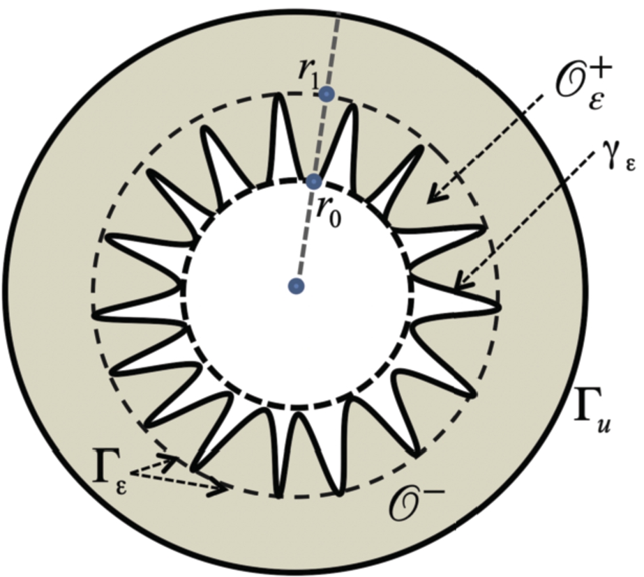
For a small parameter $ε = \frac{2 π}{N}$ , $N \in Z^{+}$ , we consider an oscillating boundary domain $O_{ε}$ as given in Fig. 1.

Fig. 1.

Circular oscillating domain $O_{ε}$ .

Fig. 2.

Reference domain D.

We describe the domain $O_{ε}$ and its boundaries as follows. Let $g : R \to R$ be a smooth and periodic function with period $2 π$ and η be a smooth real valued function defined on $[0, 2 π]$ such that it takes the maximum at the end points, that is, $η (0) = η (2 π) = r_{1} = : {max}_{θ \in [0, 2 π]} η (θ)$ . Also assume that the function $r_{1} - η$ is compactly supported in $(0, 2 π)$ . Now extend η to the whole real line periodically with period $2 π$ .

Let $r_{0} = : {min}_{θ \in [0, 2 π]} η (θ)$ and $m < {min}_{θ \in [0, 2 π]} g (θ)$ with $0 < r_{0} < r_{1} < m$ . Now, define the domain $O_{ε}$ as $\begin{matrix} O_{ε} = {(r, θ) \in R^{2} : 0 < θ ⩽ 2 π, η_{ε} (θ) = η (\frac{θ}{ε}) < r < g (θ)} . \end{matrix}$ Typically, $O_{ε}$ consists of an annulus type region bounded by the inner circle of radius $r_{1}$ and outer boundary given by g and an oscillating region bounded by the outer circle of radius $r_{1}$ and the oscillating inner boundary defined by $η_{ε}$ . The oscillating inner boundary of $O_{ε}$ denoted by $γ_{ε}$ is given by $γ_{ε} = {(r, θ) : θ \in [0, 2 π], r = η_{ε} (θ)}$ . The fixed outer boundary $Γ_{u}$ of $O_{ε}$ is defined by $Γ_{u} = {(r, θ) : r = g (θ), θ \in [0, 2 π]}$ . Let $O_{ε}^{+}$ be the oscillating part of the domain $O_{ε}$ , which is $O_{ε}^{+} = {(r, θ) \in R^{2} : 0 < θ ⩽ 2 π, η_{ε} (θ) < r < r_{1}}$ . The reference cell D is defined as $D = : {(r, θ) : η (θ) < r < r_{1}, 0 < θ ⩽ 2 π}$ (Fig. 2) and the reference set $Y (a)$ for $a \in [r_{0}, r_{1}]$ , is defined as $\begin{matrix} Y (a) = {θ \in (0, 2 π) : (a cos θ, a sin θ) \in \overline{D}} . \end{matrix}$ In other words, for $a \in (r_{0}, r_{1}]$ , $Y (a) = {θ \in (0, 2 π) : η (θ) < a}$ and $Y (r_{0}) = {θ \in (0, 2 π) : η (θ) = r_{0}}$ . Note that $Y (a)$ is Lebesgue measurable as η is assumed to be a smooth function and $h (a) = | Y (a) |$ , where $| Y (a) |$ is the Lebesgue measure of the set $Y (a)$ . Defining $Y (a)$ in this novel way is crucial in the definition of the unfolding operators in circular oscillating domains. We choose η in such a way that h is strictly positive in $[r_{0}, r_{1}]$ . Denote $O^{-}$ , the fixed part of the domain $O_{ε}$ , which is described by $O^{-} = {(r, θ) : 0 < θ ⩽ 2 π, r_{1} < r < g (θ)}$ . The inner boundary of $O^{-}$ denoted by $Γ_{0}$ is defined as $Γ_{0} = {(r_{1}, θ) : 0 ⩽ θ ⩽ 2 π}$ . The common boundary $Γ_{ε}$ is defined as $Γ_{ε} = {(r, θ) \in O_{ε} : r = r_{1}}$ . We can also write $O_{ε}$ as $O_{ε} = Int (\overline{O_{ε}^{+} \cup O^{-}})$ . The full domain or the limiting domain $O$ is described by $O = {(r, θ) : 0 < θ ⩽ 2 π, r_{0} < r < g (θ)}$ and the inner limit domain $O^{+}$ is given by $O^{+} = {(r, θ) : 0 < θ ⩽ 2 π, r_{0} < r < r_{1}}$ . The boundaries of $O$ are $Γ_{u}$ and $Γ_{b}$ , where $Γ_{b} = {(r_{0}, θ) : 0 ⩽ θ ⩽ 2 π}$ and $Γ_{u}$ is the same as defined earlier.

3. Unfolding operator and its properties

We now recall the relevant periodic unfolding operator $T^{ε}$ and the boundary unfolding operator $T_{r_{1}}^{ε}$ which was developed by Aiyappan, Nandakumaran and Prakash in [2] for circular oscillating domain to study homogenization problems posed on this type of domain. We also present some of its important properties which are required for our analysis in Sections 5 and 6. Let us define the unfolded (fixed) domain $O_{u}$ , where the unfolded functions are defined, as below.

Let $G = {(r, τ) : r \in (r_{0}, r_{1}), τ \in Y (r)}$ , then $O_{u}$ is defined as $O_{u} = (0, 2 π) \times G$ and it can be written as $\begin{matrix} O_{u} = : {(r, θ, τ) | 0 < θ < 2 π, r_{0} < r < r_{1}, τ \in Y (r)} . \end{matrix}$ For $x \in R$ , we write ${[x]}_{2 π}$ as the integer part of x with respect to $2 π$ , that is, ${[x]}_{2 π} = 2 k π$ , where k is the largest integer such that $2 k π ⩽ x$ and ${x}_{2 π} = x - {[x]}_{2 π}$ . We now give the definition of unfolding operator for our domain. The unfolding operator has been used to understand the various scales present in a function u. Thus the relevance of $T^{ε}$ comes into effect when $T^{ε}$ is applied on functions $u^{ε}$ with different scales x and $\frac{x}{ε}$ , like $u^{ε} (x) = u (x, \frac{x}{ε})$ . This is already available in the literature for rectangular type domains. In our case, the domain is circular and hence we define the unfolding operator in polar coordinates.

Definition 3.1 (The unfolding operator).

For each fixed $ε > 0$ , the unfolding operator $T^{ε}$ unfolds any function u defined on the oscillating domain $O_{ε}^{+}$ into another function $(T^{ε} u)$ defined on the fixed domain $O_{u}$ . More precisely, the unfolding operator $\begin{matrix} T^{ε} : {u | u : O_{ε}^{+} \to R} \to {v | v : O_{u} \to R} \end{matrix}$ is defined by $\begin{matrix} (T^{ε} u) (r, θ, τ) = u (r, ε {[\frac{θ}{ε}]}_{2 π} + ε τ) \forall u \in O_{ε}^{+} . \end{matrix}$

If U is an open subset of $R^{2}$ containing $O_{ε}^{+}$ and u is a real valued function on U, $T^{ε} u$ will mean $T^{ε}$ acting on the restriction of u to $O_{ε}^{+}$ . Some of the properties of $T^{ε}$ are given below. Though the proofs can be found in [2], we recall them in the Appendix for completeness.

Proposition 3.2.
For each fixed $ε > 0$ , $T^{ε}$ is linear and $T^{ε} (u v) = T^{ε} (u) T^{ε} (v)$ , where $u, v : O_{ε}^{+} \to R$ .
Proposition 3.3.
Let $u \in L^{1} (O_{ε}^{+})$ . Then $\begin{matrix} \int_{O_{u}} T^{ε} u r d r d θ d τ = 2 π \int_{O_{ε}^{+}} u r d r d θ . \end{matrix}$
Proposition 3.4.
Let $u \in L^{2} (O_{ε}^{+})$ . Then $T^{ε} u \in L^{2} (O_{u})$ and $‖ T^{ε} u ‖_{L^{2} (O_{u})} = \sqrt{2 π} ‖ u ‖_{L^{2} (O_{ε}^{+})}$ .
Proposition 3.5.
Let $u, \frac{\partial u}{\partial r}, \frac{\partial u}{\partial θ} \in L^{2} (O_{ε}^{+})$ . Then $T^{ε} u, \frac{\partial}{\partial r} T^{ε} u, \frac{\partial}{\partial τ} T^{ε} u \in L^{2} (O_{u})$ . Moreover, $\frac{\partial}{\partial r} T^{ε} u = T^{ε} \frac{\partial u}{\partial r}$ and $\frac{\partial}{\partial τ} T^{ε} u = ε T^{ε} \frac{\partial u}{\partial θ}$ .
Proposition 3.6.
Let $u \in L^{2} (O^{+})$ . Then $T^{ε} u \to u$ in $L^{2} (O_{u})$ . More generally, if $y_{ε} \to y$ in $L^{2} (O^{+})$ , then $T^{ε} y_{ε} \to y$ in $L^{2} (O_{u})$ .
Proposition 3.7.
For every $ε > 0$ , let $y_{ε} \in L^{2} (O_{ε}^{+})$ such that $T^{ε} y_{ε} ⇀ y$ weakly in $L^{2} (O_{u})$ . Then $\begin{matrix} {\tilde{y}}_{ε} ⇀ \frac{1}{2 π} \int_{Y (r)} y (r, θ, τ) d τ \end{matrix}$ weakly in $L^{2} (O^{+})$ . Here, ${\tilde{y}}_{ε}$ is the zero extension of $y_{ε}$ to $O^{+}$ .

We, now derive the convergence of unfolding for $H^{1}$ functions. Proposition 3.8.
Let $y_{ε} \in H^{1} (O_{ε}^{+})$ for every $ε > 0$ such that $T^{ε} y_{ε} ⇀ y$ and $\frac{\partial}{\partial r} T^{ε} y_{ε} ⇀ \frac{\partial y}{\partial r} weakly in L^{2} (O_{u})$ . Then ${\tilde{y}}_{ε} ⇀ \frac{1}{2 π} \int_{Y (r)} y d τ$ and $\tilde{\frac{\partial y_{ε}}{\partial r}} ⇀ \frac{1}{2 π} \int_{Y (r)} \frac{\partial y}{\partial r} d τ$ weakly in $L^{2} (O^{+})$ .

3.1. Unfolding on the boundary

We, now define the boundary unfolding operator on $Γ_{ε}$ , that is, on the common boundary of $O_{ε}^{+}$ and $O^{-}$ .

Definition 3.9.
Let $ϕ_{r_{1}}^{ε} : (0, 2 π) \times Y (r_{1}) \to Γ_{ε}$ be defined by $(θ, τ) \to ε {[\frac{θ}{ε}]}_{2 π} + ε τ$ . The ε-unfolding of a function $u : Γ_{ε} \to R$ is the function $u \circ ϕ_{r_{1}}^{ε} : (0, 2 π) \times Y (r_{1}) \to R$ denoted by $T_{r_{1}}^{ε}$ . That is, $\begin{matrix} T_{r_{1}}^{ε} : {u | u : Γ_{ε} \to R} \to {v | v : (0, 2 π) \times Y (r_{1}) \to R} \end{matrix}$ by $\begin{matrix} T_{r_{1}}^{ε} u = u \circ ϕ_{r_{1}}^{ε} = u (ε {[\frac{θ}{ε}]}_{2 π} + ε τ) . \end{matrix}$

If U is an open subset of $R^{2}$ such that $Γ_{ε} \subset U$ and $u : U \to R$ then $T_{r_{1}}^{ε} u = T_{r_{1}}^{ε} (u |_{Γ_{ε}})$ .

The properties of the boundary unfolding operator are given below without proof. In fact, all of them can be proved analogously as above.
Proposition 3.10.

$T_{r_{1}}^{ε}$ is linear.

Let u,v be functions from $Γ_{ε} \to R$ . Then $T_{r_{1}}^{ε} (u v) = T_{r_{1}}^{ε} (u) T_{r_{1}}^{ε} (v)$ .

Let $u \in L^{2} (Γ_{ε})$ . Then $T_{r_{1}}^{ε} u \in L^{2} ((0, 2 π) \times Y (r_{0}))$ . Moreover, $‖ T_{r_{1}}^{ε} u ‖_{L^{2} ((0, 2 π) \times Y (r_{0}))} = \sqrt{2 π} ‖ u ‖_{L^{2} (Γ_{ε})}$ .

Let $u \in H^{1} (Γ_{ε})$ . Then $T_{r_{1}}^{ε} u \in L^{2} (0, L; H^{1} (Y (r_{0})))$ and $\frac{\partial}{\partial τ} T_{r_{1}}^{ε} u = ε T_{r_{1}}^{ε} \frac{\partial u}{\partial θ}$ .

Let $u \in L^{2} (0, 2 π)$ . Then $T_{r_{1}}^{ε} u \to u$ in $L^{2} ((0, 2 π) \times Y (r_{1}))$ .

Suppose that $u_{ε} \to u$ in $L^{2} (0, 2 π)$ . Then $T_{r_{1}}^{ε} u_{ε} \to u$ in $L^{2} ((0, 2 π) \times Y (r_{1}))$ .

Suppose that $u_{ε}$ is a sequence in $L^{2} (Γ_{ε})$ such that $T_{r_{1}}^{ε} u_{ε} ⇀ u$ weakly in $L^{2} ((0, 2 π) \times Y (r_{1}))$ . Then ${\tilde{u}}_{ε} ⇀ \frac{1}{2 π} \int_{Y (r_{1})} u d τ$ weakly in $L^{2} (0, 2 π)$ .

In the next section, we describe an optimal control problem posed on this oscillating domain and study the existence and uniqueness of its solution. Also, we use the unfolding operator which we have developed, to characterize the optimal control. This is one of the main contributions of this article.
4. Optimal control problem

We consider an interior optimal control problem where the controls are coming from the fixed reference cell D and periodically distributed over $O_{ε}^{+}$ . Suppose we have the elliptic system: $\begin{matrix} (4.1) & \{\begin{matrix} - Δ y_{ε} + y_{ε} = f_{0} + χ_{O_{ε}^{+}} q^{ε} & in O_{ε}, \\ \partial_{ν} y_{ε} = 0 & on \partial O_{ε}, \end{matrix} \end{matrix}$ where $q \in L^{2} (D)$ with $q^{ε} (r, θ) = q (r, \frac{θ}{ε})$ and the source term $f_{0} \in L^{2} (O)$ . It is known that equation (4.1) admits a unique weak solution $y_{ε}$ in $H^{1} (O_{ε})$ by applying the Lax–Milgram theorem. The solution operator is linear and continuous from $L^{2} (O_{ε}) \times L^{2} (D)$ into $H^{1} (O_{ε})$ , i.e. $\begin{matrix} (4.2) & ‖ y_{ε} ‖_{H^{1} (O_{ε})} ⩽ C (‖ f_{0} ‖_{L^{2} (O)} + ‖ q ‖_{L^{2} (D)}), \end{matrix}$ where $C > 0$ is independent of ε. We define the $L^{2}$ -cost functional $J_{ε}$ as $\begin{array}{rcl} (4.3) & J_{ε} (y_{ε}, q) & = & \frac{1}{2} \int_{O_{ε}} | y_{ε} - y_{d} |^{2} r d r d θ + \frac{β}{2} \int_{O_{ε}^{+}} {| q^{ε} |}^{2} r d r d θ \end{array}$ with the desired state $y_{d} \in L^{2} (O)$ . Now, we define the optimal control problem as follows.

Find $({\overline{y}}_{ε}, {\overline{q}}_{ε}) \in H^{1} (O_{ε}) \times L^{2} (D)$ such that $\begin{array}{rcl} (P_{ε}) J_{ε} ({\overline{y}}_{ε}, {\overline{q}}_{ε}) = inf {J_{ε} (y_{ε}, q) | (y_{ε}, q) \in H^{1} (O_{ε}) \times L^{2} (D), (y_{ε}, q) satisfies (4.1)} . \end{array}$

In this section, we analyze the control problem with the $L^{2}$ -cost functional. In Section 6, we study the homogenization of the control problem with a Dirichlet cost functional. We have the following existence result for each fixed $ε > 0$ (see Raymond [30]).

Theorem 4.1.
For each $ε > 0$ , the minimization problem ( $P_{ε}$ ) admits a unique solution.

The focus of the following subsection is the derivation of the optimality system and characterization of the optimal control.
4.1. Optimality system

One of our main results is the derivation of the following optimality system and characterization of optimal control via the unfolding operator which is given in the following theorem.

Theorem 4.2.
Let $({\overline{y}}_{ε}, {\overline{q}}_{ε}) \in H^{1} (O_{ε}) \times L^{2} (D)$ be the optimal solution to ( $P_{ε}$ ), then the optimal control is characterized by $\begin{matrix} (4.4) & {\overline{q}}_{ε} (r, τ) |_{D} = \frac{- 1}{2 π β} \int_{0}^{2 π} (T^{ε} {\overline{p}}_{ε}^{+}) (r, θ, τ) d θ \end{matrix}$ where ${\overline{y}}_{ε}$ satisfies ( 4.1 ) with $q^{ε} = {\overline{q}}_{ε} (r, \frac{θ}{ε})$ and the adjoint state ${\overline{p}}_{ε}$ satisfies the problem $\begin{matrix} (4.5) & \{\begin{matrix} - Δ {\overline{p}}_{ε} + {\overline{p}}_{ε} = {\overline{y}}_{ε} - y_{d} & in O_{ε}, \\ \partial_{ν} {\overline{p}}_{ε} = 0 & on \partial O_{ε} . \end{matrix} \end{matrix}$ Conversely, if a pair $({\hat{y}}_{ε}, {\hat{p}}_{ε})$ satisfies the following system $\begin{array}{l} \{\begin{matrix} - Δ {\hat{y}}_{ε} + {\hat{y}}_{ε} = f_{0} + χ_{O_{ε}^{+}} {\hat{Q}}_{ε}; - Δ {\hat{p}}_{ε} + {\hat{p}}_{ε} = {\hat{y}}_{ε} - y_{d} & in O_{ε}, \\ \partial_{ν} {\hat{y}}_{ε} = 0; \partial_{ν} {\hat{p}}_{ε} = 0 & on \partial O_{ε}, \\ {\hat{q}}_{ε} (r, τ) = \frac{- 1}{2 π β} \int_{0}^{2 π} T^{ε} {\hat{p}}_{ε}^{+} d θ & on D, \end{matrix} \end{array}$ then the pair $({\hat{y}}_{ε}, {\hat{q}}_{ε})$ is the optimal solution to $(P_{ε})$ . Here ${\hat{Q}}_{ε} (r, θ) = {\hat{q}}_{ε} (r, \frac{θ}{ε})$ .
Proof.
Given $q \in L^{2} (D)$ , let $F_{ε} (q) = J_{ε} (y_{ε} (q), q)$ , where $y_{ε} (q)$ is the solution to the equation (4.1). Set ${\overline{Q}}_{ε} (r, θ) = {\overline{q}}_{ε} (r, \frac{θ}{ε})$ .

Using appropriate computation on $\frac{1}{λ} (F_{ε} ({\overline{q}}_{ε} + λ q) - F_{ε} ({\overline{q}}_{ε}))$ and taking limit as $λ \to 0$ , we get $\begin{array}{rcl} F_{ε}^{'} ({\overline{q}}_{ε}) q & = & \int_{O_{ε}} ({\overline{y}}_{ε} - y_{d}) w_{ε} r d r d θ + β \int_{O_{ε}} χ_{O_{ε}^{+}} {\overline{Q}}_{ε} q^{ε} r d r d θ, \end{array}$ where $q^{ε} (r, θ) = q (r, \frac{θ}{ε})$ and $w_{ε}$ is the solution of the following equation $\begin{array}{l} (4.6) & \{\begin{matrix} - Δ w_{ε} + w_{ε} = χ_{O_{ε}^{+}} q^{ε} & in O_{ε}, \\ \partial_{ν} w_{ε} = 0 & on \partial O_{ε} . \end{matrix} \end{array}$ We skip the computations involved and refer the reader to [1,25] for detailed computations.

Since $({\overline{y}}_{ε}, {\overline{q}}_{ε})$ is an optimal solution to $(P_{ε})$ , we have $F_{ε}^{'} ({\overline{q}}_{ε}) q = 0$ for all $q \in L^{2} (D)$ , it follows that $\begin{array}{rcl} \int_{O_{ε}} ({\overline{y}}_{ε} - y_{d}) w_{ε} r d r d θ = - β \int_{O_{ε}^{+}} {\overline{Q}}_{ε} q^{ε} r d r d θ . \end{array}$ Using integration by parts in equations (4.5) and (4.6) with test functions $w_{ε}$ and ${\overline{p}}_{ε}$ , respectively, we get $\begin{array}{l} \int_{O_{ε}} ({\overline{y}}_{ε} - y_{d}) w_{ε} r d r d θ = \int_{O_{ε}^{+}} {\overline{p}}_{ε}^{+} q^{ε} r d r d θ \\ ⟹ - β \int_{O_{ε}^{+}} {\overline{Q}}_{ε} q^{ε} r d r d θ = \int_{O_{ε}^{+}} {\overline{p}}_{ε}^{+} q^{ε} r d r d θ, \forall q \in L^{2} (D) . \end{array}$ Now, note that $T^{ε} ({\overline{Q}}_{ε}) (r, θ, τ) = {\overline{q}}_{ε} (r, τ)$ and ${\overline{q}}_{ε} |_{D} ⇀ {\overline{q}}_{0} |_{D}$ weakly in $L^{2} (D)$ . Applying the unfolding operator we get, $\begin{array}{rcl} \int_{O_{ε}^{+}} {\overline{Q}}_{ε} q^{ε} r d r d θ = \frac{1}{2 π} \int_{O_{u}} T^{ε} {\overline{Q}}_{ε} T^{ε} q^{ε} r d r d θ d τ = \frac{1}{2 π} \int_{O_{u}} {\overline{q}}_{ε} q r d r d θ d τ = \int_{D} {\overline{q}}_{ε} q r d r d τ . \end{array}$ Similarly, $\begin{array}{rcl} \int_{O_{ε}^{+}} {\overline{p}}_{ε} q^{ε} r d r d θ & = & \frac{1}{2 π} \int_{O_{u}} T^{ε} {\overline{p}}_{ε}^{+} T^{ε} q^{ε} r d r d θ d τ = \frac{1}{2 π} \int_{O_{u}} T^{ε} {\overline{p}}_{ε}^{+} q r d r d θ d τ \\ = & \int_{D} (\frac{1}{2 π} \int_{0}^{2 π} T^{ε} {\overline{p}}_{ε}^{+} d θ) q r d r d τ . \end{array}$ Since this is valid for all $q \in L^{2} (D)$ , we get $\begin{matrix} {\overline{q}}_{ε} = - \frac{1}{2 π β} [\int_{0}^{2 π} T^{ε} {\overline{p}}_{ε}^{+} d θ] a.e. in D . \end{matrix}$ The converse can be proved easily with a reverse argument. □

The section that follows describes the homogenization of this control problem which is one of the main contributions of this paper.
5. Homogenization

Recall $h (r) = | Y (r) |$ , where $| Y (r) |$ is the Lebesgue measure of the set $Y (r)$ at $r \in [r_{0}, r_{1}]$ . Note that h is a strictly positive function in $[r_{0}, r_{1}]$ . Let ψ be any function defined on $O$ , then ψ can be written as $ψ = ψ^{+} χ_{O^{+}} + ψ^{-} χ_{O^{-}}$ where $ψ^{+} = ψ |_{O^{+}}$ and $ψ^{-} = ψ |_{O^{-}}$ . Now, consider the anisotropic Sobolev space $\begin{matrix} W (O) = {ψ \in L^{2} (O) : \frac{\partial ψ}{\partial r} \in L^{2} (O), ψ^{-} \in H^{1} (O^{-})} . \end{matrix}$ Note that $W (O)$ is a Hilbert space with the inner product $\begin{array}{rcl} {⟨ u, v ⟩}_{W} & = & {⟨ h u, v ⟩}_{L^{2} (O^{+})} + {⟨ h \partial_{r} u, \partial_{r} v ⟩}_{L^{2} (O^{+})} + {⟨ \partial_{r} u, \partial_{r} v ⟩}_{L^{2} (O^{-})} \\ + {⟨ \frac{1}{r^{2}} \partial_{θ} u, \partial_{θ} v ⟩}_{L^{2} (O^{-})} + {⟨ u, v ⟩}_{L^{2} (O^{-})}, \end{array}$ where $\begin{matrix} {⟨ u, v ⟩}_{L^{2} (A)} = : \int_{A} u v r d r d θ \forall A \subseteq O . \end{matrix}$ Given $f_{0} \in L^{2} (O)$ and $q \in L^{2} (r_{0}, r_{1})$ , consider the limit state equation: $\begin{array}{l} (5.1) & \{\begin{matrix} - \frac{\partial}{\partial r} (h (r) \frac{\partial y^{+}}{\partial r}) - \frac{h (r)}{r} \frac{\partial y^{+}}{\partial r} + h (r) y^{+} = h (r) (f_{0}^{+} + q χ_{O^{+}}) & in O^{+}, \\ - Δ y^{-} + y^{-} = f_{0}^{-} & in O^{-}, \\ \frac{\partial y^{+}}{\partial ν} = 0 & on \partial O, \\ y^{+} = y^{-}, \frac{h (r_{1})}{2 π} \frac{\partial y^{+}}{\partial r} = \frac{\partial y^{-}}{\partial r} & in Γ_{0} . \end{matrix} \end{array}$ The weak formulation of the above equation is given below.

Find $y \in W (O)$ such that $\begin{array}{l} \int_{O^{+}} \frac{h (r)}{2 π} (\frac{\partial y^{+}}{\partial r} \frac{\partial ψ^{+}}{\partial r} + y^{+} ψ^{+}) r d r d θ + \int_{O^{-}} (\frac{\partial y^{-}}{\partial r} \frac{\partial ψ^{-}}{\partial r} + \frac{1}{r^{2}} \frac{\partial y^{-}}{\partial θ} \frac{\partial ψ^{-}}{\partial θ} + y^{-} ψ^{-}) r d r d θ \\ = \int_{O^{+}} \frac{h (r)}{2 π} (f_{0}^{+} + q) ψ^{+} r d r d θ + \int_{O^{-}} f_{0}^{-} ψ^{-} r d r d θ, \end{array}$ for all $ψ \in W (O)$ . By Lax–Milgram theorem, there exists a unique weak solution in $W (O)$ to problem (5.1) and the solution operator is linear and continuous. Also we have the following a priori estimate: $\begin{array}{rcl} (5.2) & ‖ y ‖_{W (O)} ⩽ C (‖ f ‖_{L^{2} (O)} + ‖ q ‖_{L^{2} (r_{0}, r_{1})}) . \end{array}$ Now, we will state the limit optimal control problem.

Find $(\overline{y}, \overline{q}) \in W (O) \times L^{2} (r_{0}, r_{1})$ such that $\begin{array}{rcl} (P) J (\overline{y}, \overline{q}) = inf {J (y, q) | (u, q) \in W (O) \times L^{2} (r_{0}, r_{1}), (y, q) satisfies (5.1)}, \end{array}$ where the cost functional J is defined as $\begin{array}{rcl} J (y, q) & = & \frac{1}{2} \int_{O^{-}} {| y^{-} - y_{d} |}^{2} r d r d θ + \frac{1}{4 π} \int_{O^{+}} h (r) {| y^{+} - y_{d} |}^{2} r d r d θ + \frac{β}{2} \int_{r_{0}}^{r_{1}} h (r) | q |^{2} r d r . \end{array}$ The following result can be easily verified as in the previous section.

Theorem 5.1.
The optimal control problem (P) has a unique solution.

Now, we will establish the optimality system for the limit problem. The adjoint state $\overline{p} \in W (O)$ solves $\begin{array}{l} (5.3) & \{\begin{matrix} - \frac{\partial}{\partial r} (h (r) \frac{\partial {\overline{p}}^{+}}{\partial r}) - \frac{h (r)}{r} \frac{\partial {\overline{p}}^{+}}{\partial r} + h (r) {\overline{p}}^{+} = h (r) ({\overline{y}}^{+} - y_{d}) & in O^{+}, \\ - Δ {\overline{p}}^{-} + {\overline{p}}^{-} = ({\overline{y}}^{-} - y_{d}) & in O^{-}, \\ \frac{\partial \overline{p}}{\partial ν} = 0 & on \partial O, \\ {\overline{p}}^{+} = {\overline{p}}^{-}, \frac{h (r_{1})}{2 π} \frac{\partial {\overline{p}}^{+}}{\partial r} = \frac{\partial {\overline{p}}^{-}}{\partial r} & on Γ_{0} . \end{matrix} \end{array}$
Theorem 5.2.
If $(\overline{y}, \overline{q})$ is an optimal solution to (P), then $\begin{matrix} \overline{q} = \frac{- 1}{2 π β} \int_{0}^{2 π} {\overline{p}}^{+} d θ, \end{matrix}$ where $\overline{p} \in W (O)$ is the solution to the adjoint problem ( 5.3 ). Conversely, assume that the pair $(\hat{y}, \hat{p}) \in W (O) \times W (O)$ solves the optimality system $\begin{matrix} (5.4) & \{\begin{matrix} - \frac{\partial}{\partial r} (h (r) \frac{\partial {\hat{y}}^{+}}{\partial r}) - \frac{h (r)}{r} \frac{\partial {\hat{y}}^{+}}{\partial r} + h (r) {\hat{y}}^{+} = h (r) (f_{0}^{+} + \hat{q}) & in O^{+}, \\ - \frac{\partial}{\partial r} (h (r) \frac{\partial {\hat{p}}^{+}}{\partial r}) - \frac{h (r)}{r} \frac{\partial {\hat{p}}^{+}}{\partial r} + h (r) {\hat{p}}^{+} = h (r) ({\hat{y}}^{+} - y_{d}) & in O^{+}, \\ - Δ {\hat{y}}^{-} + {\hat{y}}^{-} = f_{0}^{-}; Δ {\hat{p}}^{-} + {\hat{p}}^{-} = ({\hat{y}}^{-} - y_{d}) & in O^{-}, \\ \frac{\partial \hat{y}}{\partial ν} = 0; \frac{\partial \hat{p}}{\partial ν} = 0 & in \partial O, \\ {\hat{y}}^{+} = {\hat{y}}^{-}, \frac{h (r_{1})}{2 π} \frac{\partial {\hat{y}}^{+}}{\partial r} = \frac{\partial {\hat{y}}^{-}}{\partial r}; {\hat{p}}^{+} = {\hat{p}}^{-}, \frac{h (r_{1})}{2 π} \frac{\partial {\hat{p}}^{+}}{\partial r} = \frac{\partial {\hat{p}}^{-}}{\partial r} & on Γ_{0}, \\ \hat{q} = \frac{- 1}{2 π β} \int_{0}^{2 π} {\hat{p}}^{+} d θ, \end{matrix} \end{matrix}$ then the pair $(\hat{y}, \hat{q})$ is the optimal solution to $(P)$ .

The theorem can be proved by following the similar steps of Theorem 4.2. For completeness, we give the proof in the appendix. Now, we will describe the main homogenization result in the following subsection.
5.1. Convergence analysis

The homogenization of the optimal control problem $P_{ε}$ is analyzed by changing the problem into polar coordinates and applying the unfolding operator. The weak form of the state equation is given in the following definition.

Definition 5.3.
We say the function $y_{ε}$ is a weak solution of the state equation (4.1) if $y_{ε}$ satisfies $\begin{array}{rcl} \int_{O_{ε}} (\frac{\partial y_{ε}}{\partial r} \frac{\partial ψ}{\partial r} + \frac{1}{r^{2}} \frac{\partial y_{ε}}{\partial θ} \frac{\partial ψ}{\partial θ} + y_{ε} ψ) r d r d θ & = & \int_{O_{ε}} (f_{0} + χ_{O_{ε}^{+}} {\overline{Q}}_{ε}) ψ r d r d θ, \end{array}$ for all $ψ \in H^{1} (O_{ε})$ .

In this subsection, we describe the homogenization of the optimal control problem. Assume that $({\overline{y}}_{ε}, {\overline{q}}_{ε})$ is the optimal solution to problem $(P_{ε})$ . Let $y_{ε} (0)$ be the solution to problem (4.1) corresponding to $q_{ε} = 0$ , then from (4.2), we get $‖ y_{ε} (0) ‖_{H^{1} (O_{ε})} ⩽ C$ , where $C > 0$ is independent of ε. Using optimality of the solution $({\overline{y}}_{ε}, {\overline{q}}_{ε})$ , we get $\begin{matrix} \frac{1}{2} \int_{O_{ε}} {({\overline{y}}_{ε} - y_{d})}^{2} r d r d θ + \frac{β}{2} \int_{O_{ε}^{+}} | {\overline{Q}}_{ε} |^{2} r d r d θ ⩽ C . \end{matrix}$ Thus, we have $\begin{matrix} (5.5) & ‖ {\overline{Q}}_{ε} ‖_{L^{2} (O_{ε}^{+})} = ‖ {\overline{q}}_{ε} ‖_{L^{2} (D)} ⩽ C and ‖ {\overline{y}}_{ε} ‖_{L^{2} (O_{ε})} ⩽ C . \end{matrix}$ Further, ${\overline{p}}_{ε}$ satisfies $‖ {\overline{p}}_{ε} ‖_{H^{1} (O_{ε})} ⩽ C$ . The zero extension of a function φ defined on $O_{ε}^{+}$ to $O^{+}$ is denoted by $\tilde{φ}$ . That is, $\begin{array}{l} \tilde{φ} = \{\begin{matrix} φ & in O_{ε}^{+} \\ 0 & in O^{+} ∖ O_{ε}^{+} . \end{matrix} \end{array}$

Now, we prove the main theorem of this section. Theorem 5.4.
Let $({\overline{y}}_{ε}, {\overline{q}}_{ε})$ and $(\overline{y}, \overline{q})$ be the optimal solutions to ( $P_{ε}$ ) and (P), respectively. Then $\begin{array}{rcl} \tilde{{\overline{y}}_{ε}^{+}} & ⇀ & \frac{h (r)}{2 π} {\overline{y}}^{+}, \tilde{\frac{\partial {\overline{y}}_{ε}^{+}}{\partial r}} ⇀ \frac{h (r)}{2 π} \frac{\partial {\overline{y}}^{+}}{\partial r} weakly in L^{2} (O^{+}), \\ (5.6) & \tilde{{\overline{p}}_{ε}^{+}} & ⇀ & \frac{h (r)}{2 π} {\overline{p}}^{+}, \tilde{\frac{\partial {\overline{p}}_{ε}^{+}}{\partial r}} ⇀ \frac{h (r)}{2 π} \frac{\partial {\overline{p}}^{+}}{\partial r} weakly in L^{2} (O^{+}), and \\ {\overline{y}}_{ε}^{-} & ⇀ & {\overline{y}}_{0}^{-}, {\overline{p}}_{ε}^{-} ⇀ {\overline{p}}^{-} weakly in H^{1} (O^{-}), \end{array}$ where $\overline{q} = \frac{- 1}{2 π β} \int_{0}^{2 π} {\overline{p}}^{+} d θ$ and ${\overline{p}}_{ε}$ , $\overline{p}$ are the solutions of ( 4.5 ) and ( 5.3 ), respectively.
Proof.
Since the sequence ${\overline{q}}_{ε}$ is bounded in $L^{2} (D)$ (by the estimate (5.5)), by weak compactness, there exists a subsequence (still denoted by ε) and $q_{0}$ such that ${\overline{q}}_{ε} ⇀ q_{0}$ weakly in $L^{2} (D)$ . Recall the continuity estimate (ref. (4.2)) of the state solution ${\overline{y}}_{ε}$ , that is, $\begin{matrix} (5.7) & ‖ {\overline{y}}_{ε} ‖_{H^{1} (O_{ε})} ⩽ C (‖ f_{0} ‖_{L^{2} (O)} + ‖ {\overline{q}}_{ε} ‖_{L^{2} (D)}), \end{matrix}$ where $C > 0$ is independent of ε. Let us estimate $T^{ε} {\overline{y}}_{ε}^{+}$ and its derivatives in the space $L^{2} (O_{u})$ . By the Proposition 3.4, we get $\begin{array}{l} {‖ T^{ε} y_{ε} ‖}_{L^{2} (O_{u})} = \sqrt{2 π} ‖ y_{ε} ‖_{L^{2} (O_{ε}^{+})}, \\ {‖ T^{ε} \frac{\partial y_{ε}}{\partial r} ‖}_{L^{2} (O_{u})} = \sqrt{2 π} {‖ \frac{\partial y_{ε}}{\partial r} ‖}_{L^{2} (O_{ε}^{+})}, and \\ {‖ T^{ε} \frac{\partial y_{ε}}{\partial τ} ‖}_{L^{2} (O_{u})} = ε \sqrt{2 π} {‖ \frac{\partial y_{ε}}{\partial θ} ‖}_{L^{2} (O_{ε}^{+})} . \end{array}$ By the weak compactness, there exists a subsequence (still denoted by ε) such that $\begin{array}{l} (5.8) & T^{ε} {\overline{y}}_{ε}^{+} ⇀ y_{0}^{+} weakly in L^{2} (O_{u}), \\ (5.9) & \frac{\partial}{\partial r} T^{ε} {\overline{y}}_{ε}^{+} ⇀ \frac{\partial y_{0}^{+}}{\partial r}, that is, T^{ε} \frac{\partial {\overline{y}}_{ε}^{+}}{\partial r} ⇀ \frac{\partial y_{0}^{+}}{\partial r} weakly in L^{2} (O_{u}), and \\ (5.10) & \frac{\partial}{\partial τ} T^{ε} {\overline{y}}_{ε}^{+} ⇀ \frac{\partial y_{0}^{+}}{\partial τ}, that is, ε T^{ε} \frac{\partial {\overline{y}}_{ε}^{+}}{\partial θ} ⇀ \frac{\partial y_{0}^{+}}{\partial τ} weakly in L^{2} (O_{u}) . \end{array}$ From the Proposition 3.5, we have $\begin{array}{l} {‖ T^{ε} \frac{\partial {\overline{y}}_{ε}^{+}}{\partial θ} ‖}_{L^{2} (O_{u})} = \sqrt{2 π} {‖ \frac{\partial {\overline{y}}_{ε}^{+}}{\partial θ} ‖}_{L^{2} (O_{ε}^{+})} ⩽ \sqrt{2 π} ‖ {\overline{y}}_{ε} ‖_{H^{1} (O_{ε})} . \end{array}$ The above estimate implies the boundedness of the sequence $T^{ε} \frac{\partial {\overline{y}}_{ε}^{+}}{\partial θ}$ in the space $L^{2} (O_{u})$ . From convergence (5.10), it follows that $\frac{\partial y_{0}^{+}}{\partial τ} = 0$ . Hence, we conclude that $\begin{matrix} (5.11) & \tilde{{\overline{y}}_{ε}^{+}} ⇀ \frac{1}{2 π} \int_{Y (r)} y_{0}^{+} d τ and \tilde{\frac{\partial {\overline{y}}_{ε}^{+}}{\partial r}} ⇀ \frac{1}{2 π} \int_{Y (r)} \frac{\partial y_{0}^{+}}{\partial r} d τ weakly in L^{2} (O^{+}) \end{matrix}$ with the help of Proposition 3.8. Since $y_{0}^{+}$ is independent of τ, we write $\begin{array}{rcl} (5.12) & \int_{Y (r)} y_{0}^{+} d τ = h (r) y_{0}^{+} and \int_{Y (r)} \frac{\partial y_{0}^{+}}{\partial r} d τ = h (r) \frac{\partial y_{0}^{+}}{\partial r} . \end{array}$ Thus, (5.11) becomes $\begin{matrix} (5.13) & \tilde{{\overline{y}}_{ε}^{+}} ⇀ \frac{h (r)}{2 π} y_{0}^{+} and \tilde{\frac{\partial {\overline{y}}_{ε}^{+}}{\partial r}} ⇀ \frac{h (r)}{2 π} \frac{\partial y_{0}^{+}}{\partial r} weakly in L^{2} (O^{+}) . \end{matrix}$ Recall that $T^{ε} \frac{\partial {\overline{y}}_{ε}^{+}}{\partial θ}$ is bounded in $L^{2} (O_{u})$ . Hence, by the weak compactness, there is an element $P \in L^{2} (O_{u})$ such that up to a subsequence (still denoted by ε), $\begin{array}{rcl} (5.14) & T^{ε} \frac{\partial {\overline{y}}_{ε}^{+}}{\partial θ} ⇀ P weakly in L^{2} (O_{u}) . \end{array}$

Using the estimate for $‖ {\overline{y}}_{ε} ‖_{H^{1} (O_{ε})}$ , we have the boundedness of ${\overline{y}}_{ε}^{-}$ in the space $H^{1} (O^{-})$ . Thus, up to a subsequence (still denoted by ε) $\begin{matrix} (5.15) & {\overline{y}}_{ε}^{-} ⇀ y_{0}^{-} weakly in H^{1} (O^{-}) . \end{matrix}$ Define, $y_{0}$ as $\begin{array}{rcl} (5.16) & y_{0} (x) = \{\begin{matrix} y_{0}^{+} & if x \in O^{+}, \\ y_{0}^{-} & if x \in O^{-} . \end{matrix} \end{array}$

Claim: $y_{0} \in W (O)$ .

We know that $y_{0} \in L^{2} (O)$ and $\frac{\partial y_{0}}{\partial r} \in L^{2} (O^{-})$ . To prove $y_{0} \in W (O)$ , we need to show $\frac{\partial y_{0}}{\partial r} \in L^{2} (O)$ . Note that $y_{0}^{+}$ is independent of τ and so is $\frac{\partial y_{0}^{+}}{\partial r}$ . Hence, we have $\frac{\partial y_{0}^{+}}{\partial r} \in L^{2} (O^{+})$ and also $\frac{\partial y_{0}}{\partial r} \in L^{2} (O^{-})$ . Thus, to show that $\frac{\partial y_{0}}{\partial r} \in L^{2} (O)$ , it is enough to prove that the trace of $y_{0}^{+}$ and $y_{0}^{-}$ are equal on $Γ_{0}$ . Since ${\overline{y}}_{ε}^{+} |_{Γ_{ε}} = {\overline{y}}_{ε}^{-} |_{Γ_{ε}}$ implies the equality of the traces for the boundary unfolding operator. More precisely, we have $T_{r_{1}}^{ε} ({\overline{y}}_{ε}^{+} |_{Γ_{ε}}) = T_{r_{1}}^{ε} ({\overline{y}}_{ε}^{-} |_{Γ_{ε}})$ i.e. $\begin{array}{rcl} (5.17) & (T^{ε} ({\overline{y}}_{ε}^{+})) |_{r = r_{1}} = T_{r_{1}}^{ε} ({\overline{y}}_{ε}^{-} |_{Γ_{ε}}) . \end{array}$ From the weak continuity of the trace operator, we can write $\begin{matrix} (T^{ε} ({\overline{y}}_{ε}^{+})) |_{r = r_{1}} ⇀ y_{0}^{+} |_{r = r_{1}} weakly in L^{2} ((0, 2 π) \times Y (r_{0})) \end{matrix}$ and from (5.15), we get $\begin{matrix} {\overline{y}}_{ε}^{-} |_{r = r_{1}} \to y_{0}^{-} |_{r = r_{1}} strongly in L^{2} (0, 2 π) . \end{matrix}$ This implies $\begin{matrix} T_{r_{1}}^{ε} ({\overline{y}}_{ε}^{-} |_{r = r_{1}}) \to y_{0}^{-} |_{r = r_{1}} in L^{2} ((0, 2 π) \times Y (r_{1})) . \end{matrix}$ Passing to the limit in (5.17) as $ε \to 0$ we get $\begin{matrix} y_{0}^{+} |_{r = r_{1}} = y_{0}^{-} |_{r = r_{1}} in L^{2} (0, 2 π), \end{matrix}$ since $y_{0}^{+}$ and $y_{0}^{-}$ are independent of τ.

Identification of the limit P in (5.14). Finally, we identify P which is identically zero.

For $ϕ \in D (O^{+})$ and $ζ (z) \in D (0, 2 π)$ , choose $ψ \in D (0, 2 π)$ such that $ψ^{'} (z) = ζ (z)$ . Now choose a test function $\begin{matrix} ϕ^{ε} (r, θ) = ε ϕ (r, θ) ψ ({\frac{θ}{ε}}), \end{matrix}$ in such a way that $ϕ^{ε}$ is continuous on $O_{ε}^{+}$ . From the definition of the ε-unfolding of $ϕ^{ε}$ and by Proposition 3.5, we get $\begin{array}{l} T^{ε} ϕ^{ε} = ε ϕ (r, ε [\frac{θ}{ε}] + ε τ) ψ (τ), \\ T^{ε} \frac{\partial ϕ^{ε}}{\partial θ} = \frac{1}{ε} \frac{\partial}{\partial τ} T^{ε} ϕ^{ε} = ε \frac{\partial ϕ}{\partial θ} (r, ε [\frac{θ}{ε}] + ε τ) ψ (τ) + ϕ (r, ε [\frac{θ}{ε}] + ε τ) ψ^{'} (τ) and \\ T^{ε} \frac{\partial ϕ^{ε}}{\partial r} = ε \frac{\partial ϕ}{\partial r} (r, ε [\frac{θ}{ε}] + ε τ) ψ (τ) . \end{array}$ From the above equations, we derive the following convergences as $ε \to 0$ : $\begin{array}{rcl} T^{ε} ϕ^{ε} \to 0, T^{ε} \frac{\partial ϕ^{ε}}{\partial θ} \to ϕ (r, θ) ψ^{'} (τ), and T^{ε} \frac{\partial ϕ^{ε}}{\partial r} \to 0 in L^{2} (O_{u}) . \end{array}$ Let us recall the variational formulation of (4.1) with the test function $ϕ^{ε}$ given by $\begin{array}{rcl} (5.18) & \int_{O_{ε}} (\frac{\partial {\overline{y}}_{ε}}{\partial r} \frac{\partial ϕ^{ε}}{\partial r} + \frac{1}{r^{2}} \frac{\partial {\overline{y}}_{ε}}{\partial θ} \frac{\partial ϕ^{ε}}{\partial θ} + {\overline{y}}_{ε} ϕ^{ε}) r d r d θ = \int_{O_{ε}} (f_{0} + χ_{O_{ε}^{+}} {\overline{Q}}_{ε}) ϕ^{ε} r d r d θ \end{array}$ Notice that $\begin{array}{l} (5.19) & \begin{matrix} \int_{O_{ε}} (\frac{\partial {\overline{y}}_{ε}}{\partial r} \frac{\partial ϕ^{ε}}{\partial r} + \frac{1}{r^{2}} \frac{\partial {\overline{y}}_{ε}}{\partial θ} \frac{\partial ϕ^{ε}}{\partial θ}) r d r d θ \\ = \int_{O_{ε}^{+}} (\frac{\partial {\overline{y}}_{ε}^{+}}{\partial r} \frac{\partial ϕ^{ε}}{\partial r} + \frac{1}{r^{2}} \frac{\partial {\overline{y}}_{ε}^{+}}{\partial θ} \frac{\partial ϕ^{ε}}{\partial θ}) r d r d θ \\ = \frac{1}{2 π} \int_{O_{u}} (T^{ε} \frac{\partial {\overline{y}}_{ε}^{+}}{\partial r} T^{ε} \frac{\partial ϕ^{ε}}{\partial r} + \frac{1}{r^{2}} T^{ε} \frac{\partial {\overline{y}}_{ε}^{+}}{\partial θ} T^{ε} \frac{\partial ϕ^{ε}}{\partial θ}) r d r d θ d τ \\ \to \frac{1}{2 π} \int_{O_{u}} P ϕ (r, θ) ψ^{'} (τ) r d r d θ d τ as ε \to 0; \end{matrix} \\ (5.20) & \int_{O_{ε}} {\overline{y}}_{ε} ϕ^{ε} r d r d θ = \int_{O_{ε}^{+}} {\overline{y}}_{ε}^{+} ϕ^{ε} r d r d θ = \frac{1}{2 π} \int_{O_{u}} T^{ε} {\overline{y}}_{ε}^{+} T^{ε} ϕ^{ε} r d r d θ d τ \to 0 as ε \to 0 \end{array}$ and $\begin{array}{rcl} \int_{O_{ε}} (f_{0} + χ_{O_{ε}^{+}} {\overline{Q}}_{ε}) ϕ^{ε} r d r d θ & = & \int_{O_{ε}^{+}} (f_{0}^{+} + {\overline{Q}}_{ε}) ϕ^{ε} r d r d θ \\ = & \frac{1}{2 π} \int_{O_{u}} T^{ε} (f_{0}^{+} + {\overline{Q}}_{ε}) T^{ε} ϕ^{ε} r d r d θ d τ \\ (5.21) & = & \frac{1}{2 π} \int_{O_{u}} (T^{ε} f_{0}^{+} + {\overline{q}}_{ε}) T^{ε} ϕ^{ε} r d r d θ d τ \to 0 as ε \to 0 . \end{array}$ Combining (5.19), (5.20) and (5.21), we get $\begin{matrix} \int_{O_{u}} P ϕ (r, θ) ψ^{'} (τ) = 0, \end{matrix}$ which implies $\begin{matrix} \int_{O^{+}} (\int_{Y (r)} P ψ^{'} (τ) d τ) ϕ (r, θ) r d r d θ = 0 \forall ϕ \in D (O^{+}) . \end{matrix}$ That is, $\begin{matrix} \int_{Y (r)} P (r, θ, τ) ψ^{'} (τ) d τ = 0 . \end{matrix}$ Hence, $\begin{matrix} \int_{Y (r)} P (r, θ, τ) ζ (τ) d τ = 0 a.e. in O^{+}, \forall ζ \in D (0, 2 π) . \end{matrix}$ Thus, $P \equiv 0$ a.e. on $O^{+}$ .

Claim: $y_{0}$ satisfies the limit equation. Choose a test function $ψ \in C^{\infty} (\overline{O})$ in the variational formulation of the polar form of (5.1), which is given by $\begin{array}{l} \int_{O_{ε}} (\frac{\partial {\overline{y}}_{ε}}{\partial r} \frac{\partial ψ}{\partial r} + \frac{1}{r^{2}} \frac{\partial {\overline{y}}_{ε}}{\partial θ} \frac{\partial ψ}{\partial θ} + {\overline{y}}_{ε} ψ) r d r d θ \\ : = \int_{O_{ε}^{+}} (\frac{\partial {\overline{y}}_{ε}^{+}}{\partial r} \frac{\partial ψ^{+}}{\partial r} + \frac{1}{r^{2}} \frac{\partial {\overline{y}}_{ε}^{+}}{\partial θ} \frac{\partial ψ^{+}}{\partial θ} + {\overline{y}}_{ε}^{+} ψ^{+}) r d r d θ \\ + \int_{O^{-}} (\frac{\partial {\overline{y}}_{ε}^{-}}{\partial r} \frac{\partial ψ^{-}}{\partial r} + \frac{1}{r^{2}} \frac{\partial {\overline{y}}_{ε}^{-}}{\partial θ} \frac{\partial ψ^{-}}{\partial θ} + {\overline{y}}_{ε}^{-} ψ^{-}) r d r d θ \\ = \int_{O_{ε}} (f_{0} + χ_{O_{ε}^{+}} {\overline{Q}}_{ε}) ψ r d r d θ \end{array}$ First, let us look at the integral on $O_{ε}^{+}$ . As $ε \to 0$ , we get $\begin{array}{l} \int_{O_{ε}^{+}} (\frac{\partial {\overline{y}}_{ε}^{+}}{\partial r} \frac{\partial ψ^{+}}{\partial r} + \frac{1}{r^{2}} \frac{\partial {\overline{y}}_{ε}^{+}}{\partial θ} \frac{\partial ψ^{+}}{\partial θ} + {\overline{y}}_{ε}^{+} ψ^{+}) r d r d θ \\ = \frac{1}{2 π} \int_{O_{u}} (T^{ε} \frac{\partial {\overline{y}}_{ε}^{+}}{\partial r} T^{ε} \frac{\partial ψ^{+}}{\partial r} + \frac{1}{r^{2}} T^{ε} \frac{\partial {\overline{y}}_{ε}^{+}}{\partial θ} T^{ε} \frac{\partial ψ^{+}}{\partial θ} + T^{ε} {\overline{y}}_{ε}^{+} T^{ε} ψ^{+}) r d r d θ d τ \\ \to \frac{1}{2 π} \int_{O_{u}} (\frac{\partial y_{0}^{+}}{\partial r} \frac{\partial ψ^{+}}{\partial r} + y_{0}^{+} ψ^{+}) r d r d θ d τ . \end{array}$ The terms on $O^{-}$ become $\begin{array}{l} \int_{O^{-}} (\frac{\partial {\overline{y}}_{ε}^{-}}{\partial r} \frac{\partial ψ^{-}}{\partial r} + \frac{1}{r^{2}} \frac{\partial {\overline{y}}_{ε}^{-}}{\partial θ} \frac{\partial ψ^{-}}{\partial θ} + {\overline{y}}_{ε}^{-} ψ^{-}) r d r d θ \\ \to \int_{O^{-}} (\frac{\partial y_{0}^{-}}{\partial r} \frac{\partial ψ^{-}}{\partial r} + \frac{1}{r^{2}} \frac{\partial y_{0}^{-}}{\partial θ} \frac{\partial ψ^{-}}{\partial θ} + y_{0}^{-} ψ^{-}) r d r d θ \end{array}$ and on $O_{ε}$ the terms become $\begin{array}{rcl} \int_{O_{ε}} (f_{0} + χ_{O_{ε}^{+}} {\overline{Q}}_{ε}) ψ r d r d θ & = & \int_{O_{ε}^{+}} (f_{0}^{+} + {\overline{Q}}_{ε}) ψ^{+} r d r d θ + \int_{O^{-}} f_{0}^{-} ψ^{-} r d r d θ \\ = & \frac{1}{2 π} \int_{O_{u}} (T^{ε} f_{0}^{+} + T^{ε} {\overline{Q}}_{ε}) T^{ε} ψ^{+} r d r d θ d τ + \int_{O^{-}} f_{0}^{-} ψ^{-} r d r d θ \\ = & \frac{1}{2 π} \int_{O_{u}} (T^{ε} f_{0}^{+} + {\overline{q}}_{ε}) T^{ε} ψ^{+} r d r d θ d τ + \int_{O^{-}} f_{0}^{-} ψ^{-} r d r d θ \\ \to & \frac{1}{2 π} \int_{O_{u}} (f_{0}^{+} + q_{0}) ψ^{+} r d r d θ d τ + \int_{O^{-}} f_{0}^{-} ψ^{-} r d r d θ . \end{array}$ Hence, as $ε \to 0$ , the limit variational formulation becomes $\begin{array}{l} \frac{1}{2 π} \int_{O_{u}} (\frac{\partial y_{0}^{+}}{\partial r} \frac{\partial ψ^{+}}{\partial r} + y_{0}^{+} ψ^{+}) r d r d θ d τ + \int_{O^{-}} (\frac{\partial y_{0}^{-}}{\partial r} \frac{\partial ψ^{-}}{\partial r} + \frac{1}{r^{2}} \frac{\partial y_{0}^{-}}{\partial θ} \frac{\partial ψ^{-}}{\partial θ} + y_{0}^{-} ψ^{-}) r d r d θ \\ = \frac{1}{2 π} \int_{O_{u}} (f_{0}^{+} + q_{0}) ψ^{+} r d r d θ d τ + \int_{O^{-}} f_{0}^{-} ψ^{-} r d r d θ . \end{array}$ This shows that $y_{0}$ satisfies the equation $\begin{array}{l} \int_{O^{+}} \frac{h (r)}{2 π} (\frac{\partial y_{0}^{+}}{\partial r} \frac{\partial ψ^{+}}{\partial r} + y_{0}^{+} ψ^{+}) r d r d θ + \int_{O^{-}} (\frac{\partial y_{0}^{-}}{\partial r} \frac{\partial ψ^{-}}{\partial r} + \frac{1}{r^{2}} \frac{\partial y_{0}^{-}}{\partial θ} \frac{\partial ψ^{-}}{\partial θ} + y_{0}^{-} ψ^{-}) r d r d θ \\ = \int_{O^{+}} \frac{h (r)}{2 π} (f_{0}^{+} + q_{0}) ψ^{+} r d r d θ + \int_{O^{-}} f_{0}^{-} ψ^{-} r d r d θ \end{array}$ for all $ψ \in C^{\infty} (\overline{O})$ . As we know that $C^{\infty} (\overline{O})$ is dense in $W (O)$ , the above equation is true for all ψ in $W (O)$ . Therefore, $y_{0}$ satisfies (5.1). Hence, we proved the convergences in (5.13).

Similarly, we can prove the following convergences. $\begin{array}{rcl} \tilde{{\overline{p}}_{ε}^{+}} & ⇀ & \frac{h (r)}{2 π} p_{0}^{+}, \tilde{\frac{\partial {\overline{p}}_{ε}^{+}}{\partial r}} ⇀ \frac{h (r)}{2 π} \frac{\partial p_{0}^{+}}{\partial r} weakly in L^{2} (O^{+}), and \\ {\overline{y}}_{ε}^{-} & ⇀ & y_{0}^{-}, {\overline{p}}_{ε}^{-} ⇀ p_{0}^{-} weakly in H^{1} (O^{-}), \end{array}$ where $y_{0}$ satisfies (5.1) with $q = q_{0}$ and $p_{0}$ satisfies (5.3) with $\overline{y} = y_{0}$ . To prove the convergence of the optimality system, it is enough to prove $\overline{q} = q_{0}$ . Recall the optimality condition (4.4): $\begin{matrix} (5.22) & {\overline{q}}_{ε} (r, τ) |_{D} = \frac{- 1}{2 π β} \int_{0}^{2 π} (T^{ε} {\overline{p}}_{ε}^{+}) (r, θ, τ) d θ . \end{matrix}$ By the convergences of ${\overline{q}}_{ε}$ and $T^{ε} {\overline{p}}_{ε}^{+}$ as $ε \to 0$ , the equation (5.22) becomes $\begin{matrix} q_{0} (r, τ) = \frac{- 1}{2 π β} \int_{0}^{2 π} p_{0}^{+} (r, θ, τ) d θ . \end{matrix}$ By noting the fact that $p_{0}$ is independent of τ, we conclude that $q_{0}$ is also independent of the variable τ. Hence, $q_{0} = \frac{- 1}{2 π β} \int_{0}^{2 π} p_{0}^{+} d θ$ . Therefore, we get the optimality system corresponding to the minimization problem $(P)$ . Then the Theorem 5.2 says that, the optimal solution is $(y_{0}, q_{0})$ . Hence by the uniqueness, we have $\overline{y} = y_{0}$ , $\overline{p} = p_{0}$ and $\overline{q} = q_{0}$ which completes the proof. □

6. Dirichlet cost functional

In this section, we study the homogenization of the control problem with a Dirichlet cost functional $G_{ε}$ defined by $\begin{array}{rcl} (6.1) & G_{ε} (z_{ε}, ϱ) & = & \frac{1}{2} \int_{O_{ε}} | \nabla z_{ε} - \nabla z_{d} |^{2} r d r d θ + \frac{β}{2} \int_{O_{ε}^{+}} {| ϱ^{ε} |}^{2} r d r d θ \end{array}$ with $ϱ^{ε} (r, θ) = ϱ (r, \frac{θ}{ε})$ and the desired state $z_{d} \in H^{1} (O)$ . Given $ϱ \in L^{2} (D)$ and the source term $f_{0} \in L^{2} (O)$ , the function $z_{ε}$ satisfies the state equation: $\begin{array}{l} (6.2) & \{\begin{matrix} - Δ z_{ε} + z_{ε} = f_{0} + χ_{O_{ε}^{+}} ϱ^{ε} & in O_{ε}, \\ \partial_{ν} z_{ε} = 0 & on \partial O_{ε} . \end{matrix} \end{array}$ The optimal control problem with Dirichlet cost functional is described as follows.

Find $({\overline{z}}_{ε}, {\overline{ϱ}}_{ε}) \in H^{1} (O_{ε}) \times L^{2} (D)$ such that $\begin{array}{rcl} (E_{ε}) G_{ε} ({\overline{z}}_{ε}, {\overline{ϱ}}_{ε}) = inf {G_{ε} (z_{ε}, ϱ) | (z_{ε}, ϱ) \in H^{1} (O_{ε}) \times L^{2} (D), (z_{ε}, ϱ) satisfies (6.2)} \end{array}$

6.1. Optimality system

We state the necessary and sufficient conditions for the optimality and also characterize the optimal control via unfolding operator in the following theorem. The proofs of the results are either skipped or sketched as they can be proved following the similar arguments as in Section 5.

Theorem 6.1.
For each $ε > 0$ , the minimization problem ( $E_{ε}$ ) admits a unique solution. Let $({\overline{z}}_{ε}, {\overline{ϱ}}_{ε}) \in H^{1} (O_{ε}) \times L^{2} (D)$ be the optimal solution to ( $E_{ε}$ ), then the optimal control is characterized by $\begin{matrix} (6.3) & {\overline{ϱ}}_{ε} (r, τ) |_{D} = \frac{- 1}{2 π β} \int_{0}^{2 π} (T^{ε} {\overline{v}}_{ε}^{+}) (r, θ, τ) d θ \end{matrix}$ where ${\overline{z}}_{ε}$ satisfies ( 6.2 ) with $ϱ^{ε} = {\overline{P}}_{ε}$ , that is $ϱ^{ε} (r, θ) = {\overline{P}}_{ε} (r, θ) = {\overline{ϱ}}_{ε} (r, \frac{θ}{ε})$ and the adjoint state ${\overline{v}}_{ε}$ satisfies the problem $\begin{array}{l} (6.4) & \{\begin{matrix} - Δ {\overline{v}}_{ε} + {\overline{v}}_{ε} = - Δ ({\overline{z}}_{ε} - z_{d}) & in O_{ε}, \\ \partial_{ν} {\overline{v}}_{ε} = (\nabla {\overline{z}}_{ε} - \nabla z_{d}) \cdot ν & on \partial O_{ε} . \end{matrix} \end{array}$ Conversely, if a pair $({\hat{z}}_{ε}, {\hat{v}}_{ε})$ satisfies the following system $\begin{array}{l} (6.5) & \{\begin{matrix} - Δ {\hat{z}}_{ε} + {\hat{z}}_{ε} = f_{0} + χ_{O_{ε}^{+}} {\hat{P}}_{ε}; - Δ {\hat{v}}_{ε} + {\hat{v}}_{ε} = - Δ ({\hat{z}}_{ε} - z_{d}) & in O_{ε}, \\ \partial_{ν} {\hat{z}}_{ε} = 0; \partial_{ν} {\hat{v}}_{ε} = (\nabla {\hat{z}}_{ε} - \nabla z_{d}) \cdot ν & on \partial O_{ε}, \\ {\hat{ϱ}}_{ε} (r, τ) = \frac{- 1}{2 π β} \int_{0}^{2 π} T^{ε} {\hat{v}}_{ε}^{+} d θ & on D, \end{matrix} \end{array}$ then the pair $({\hat{z}}_{ε}, {\hat{ϱ}}_{ε})$ is the optimal solution to $(E_{ε})$ . Here ${\hat{P}}_{ε} (r, θ) = {\hat{ϱ}}_{ε} (r, \frac{θ}{ε})$ .

Limit problem. Now, we will describe the limit problem. Given $f_{0} \in L^{2} (O)$ and $ϱ \in L^{2} (r_{0}, r_{1})$ , consider the limit state equation: $\begin{matrix} (6.6) & \{\begin{matrix} - \frac{\partial}{\partial r} (h (r) \frac{\partial z^{+}}{\partial r}) - \frac{h (r)}{r} \frac{\partial z^{+}}{\partial r} + h (r) z^{+} = h (r) (f_{0}^{+} + ϱ χ_{O^{+}}) & in O^{+}, \\ - Δ z^{-} + z^{-} = f_{0}^{-} & in O^{-}, \\ \frac{\partial z}{\partial ν} = 0 & on \partial O, \\ z^{+} = z^{-}, \frac{h (r_{1})}{2 π} \frac{\partial z^{+}}{\partial r} = \frac{\partial z^{-}}{\partial r} & on Γ_{0}, \end{matrix} \end{matrix}$ where $\begin{array}{l} z = \{\begin{matrix} z^{+} & if x \in O^{+} \\ z^{-} & if x \in O^{-} . \end{matrix} \end{array}$ The limit optimal control problem is given below.

Find $(\overline{z}, \overline{ϱ}) \in W \times L^{2} (r_{0}, r_{1})$ such that $\begin{array}{rcl} (E) G (\overline{z}, \overline{ϱ}) = inf {J (z, ϱ) | (z, ϱ) \in W \times L^{2} (r_{0}, r_{1}), (z, ϱ) satisfies (6.6)}, \end{array}$ where the cost functional G is defined as $\begin{array}{rcl} G (z, ϱ) & = & \frac{1}{2} \int_{O^{-}} {| \nabla z^{-} - \nabla z_{d} |}^{2} r d r d θ + \frac{1}{4 π} \int_{O^{+}} h (r) {| \partial_{r} z^{+} - \partial_{r} z_{d} |}^{2} r d r d θ \\ + \frac{β}{2} \int_{r_{0}}^{r_{1}} h (r) | ϱ |^{2} r d r . \end{array}$ Now, we will establish the optimality system for this limit problem. The adjoint state $\overline{v} \in W (O)$ solves $\begin{array}{l} (6.7) & \{\begin{matrix} - \frac{\partial}{\partial r} (h (r) \frac{\partial {\overline{v}}^{+}}{\partial r}) - \frac{h (r)}{r} \frac{\partial {\overline{v}}^{+}}{\partial r} + h (r) {\overline{v}}^{+} = - \frac{\partial}{\partial r} (h (r) \frac{\partial ({\overline{z}}^{+} - z_{d})}{\partial r}) - \frac{h (r)}{r} \frac{\partial ({\overline{z}}^{+} - z_{d})}{\partial r} & in O^{+}, \\ - Δ {\overline{v}}^{-} + {\overline{v}}^{-} = - Δ ({\overline{z}}^{-} - z_{d}) & in O^{-}, \\ \frac{\partial {\overline{v}}^{+}}{\partial ν} = \frac{\partial}{\partial r} ({\overline{z}}^{+} - z_{d}) & on Γ_{b}, \\ \frac{\partial {\overline{v}}^{-}}{\partial ν} = \frac{\partial}{\partial ν} ({\overline{z}}^{-} - z_{d}) & on Γ_{u}, \\ {\overline{v}}^{+} = {\overline{v}}^{-}, \frac{h (r_{1})}{2 π} \frac{\partial {\overline{v}}^{+}}{\partial r} = \frac{\partial {\overline{v}}^{-}}{\partial r} & on Γ_{0} . \end{matrix} \end{array}$ The following result can be easily verified as in the previous section. Theorem 6.2.
The optimal control problem $(E)$ has a unique solution. If $(\overline{z}, \overline{ϱ})$ is an optimal solution to $(E)$ , then $\begin{matrix} (6.8) & \overline{ϱ} = \frac{- 1}{2 π β} \int_{0}^{2 π} {\overline{v}}^{+} d θ \end{matrix}$ where $\overline{v} \in W (O)$ is the solution to the adjoint problem ( 6.7 ). The converse is also true (similar to Theorem 5.2 ).
Theorem 6.3.
Let $({\overline{z}}_{ε}, {\overline{ϱ}}_{ε})$ and $(\overline{z}, \overline{ϱ})$ be the optimal solutions to ( $E_{ε}$ ) and (E), respectively. Then $\begin{array}{rcl} \tilde{{\overline{z}}_{ε}^{+}} & ⇀ & \frac{h (r)}{2 π} {\overline{z}}^{+}, \tilde{\frac{\partial {\overline{z}}_{ε}^{+}}{\partial r}} ⇀ \frac{h (r)}{2 π} \frac{\partial {\overline{z}}^{+}}{\partial r} weakly in L^{2} (O^{+}), \\ (6.9) & \tilde{{\overline{v}}_{ε}^{+}} & ⇀ & \frac{h (r)}{2 π} {\overline{v}}^{+}, \tilde{\frac{\partial {\overline{v}}_{ε}^{+}}{\partial r}} ⇀ \frac{h (r)}{2 π} \frac{\partial {\overline{v}}^{+}}{\partial r} weakly in L^{2} (O^{+}), and \\ {\overline{z}}_{ε}^{-} & ⇀ & {\overline{z}}^{-}, {\overline{v}}_{ε}^{-} ⇀ {\overline{v}}^{-} weakly in H^{1} (O^{-}), \end{array}$ where $\overline{ϱ} = \frac{- 1}{2 π β} \int_{0}^{2 π} {\overline{v}}^{+} d θ$ and ${\overline{v}}_{ε}$ , $\overline{v}$ are the solutions of ( 6.4 ) and ( 6.7 ), respectively.
Proof.
As in the proof of Theorem 5.4, we get $\begin{array}{rcl} \tilde{{\overline{z}}_{ε}^{+}} & ⇀ & \frac{h (r)}{2 π} z_{0}^{+}, \tilde{\frac{\partial {\overline{z}}_{ε}^{+}}{\partial r}} ⇀ \frac{h (r)}{2 π} \frac{\partial z_{0}^{+}}{\partial r} weakly in L^{2} (O^{+}), and \\ {\overline{z}}_{ε}^{-} & ⇀ & z_{0}^{-} weakly in H^{1} (O^{-}) . \end{array}$ Now, we look at the convergence of the adjoint state ${\overline{v}}_{ε}$ . As the state ${\overline{z}}_{ε}$ is uniformly bounded, we get $\begin{matrix} (6.10) & ‖ {\overline{v}}_{ε} ‖_{H^{1} (O_{ε})} ⩽ C ({\overline{z}}_{ε} ‖_{H^{1} (O_{ε})} + ‖ z_{d} ‖_{H^{1} (O)}) ⩽ C, \end{matrix}$ where $C > 0$ is independent of ε. Using this estimate and following the similar arguments of Theorem 5.4, we get the following convergences: $\begin{matrix} (6.11) & \tilde{{\overline{v}}_{ε}^{+}} ⇀ \frac{h (r)}{2 π} v_{0}^{+} and \tilde{\frac{\partial {\overline{v}}_{ε}^{+}}{\partial r}} ⇀ \frac{h (r)}{2 π} \frac{\partial v_{0}^{+}}{\partial r} weakly in L^{2} (O^{+}) . \end{matrix}$ Also, we know that $T^{ε} \frac{\partial {\overline{v}}_{ε}^{+}}{\partial θ}$ is bounded in $L^{2} (O_{u})$ . Hence, by the weak compactness, there is an element $R \in L^{2} (O_{u})$ such that up to subsequence (still denoted by ε), $\begin{array}{rcl} T^{ε} \frac{\partial {\overline{v}}_{ε}^{+}}{\partial θ} ⇀ R weakly in L^{2} (O_{u}) . \end{array}$ Using the estimate for $‖ {\overline{v}}_{ε} ‖_{H^{1} (O_{ε})}$ , we have the boundedness of ${\overline{v}}_{ε}^{-}$ in the space $H^{1} (O^{-})$ . Thus, up to a subsequence (still denoted by ε) $\begin{matrix} (6.12) & {\overline{v}}_{ε}^{-} ⇀ v_{0}^{-} weakly in H^{1} (O^{-}) . \end{matrix}$ Define $v_{0}$ as $\begin{array}{rcl} (6.13) & v_{0} (x) = \{\begin{matrix} v_{0}^{+} & if x \in O^{+}, \\ v_{0}^{-} & if x \in O^{-} . \end{matrix} \end{array}$

Identification of the limit R. We choose the same test function $ϕ^{ε}$ as in Theorem 5.4 which satisfies, as $ε \to 0$ , $\begin{array}{rcl} T^{ε} ϕ^{ε} \to 0, T^{ε} \frac{\partial ϕ^{ε}}{\partial θ} \to ϕ (r, θ) ψ^{'} (τ), and T^{ε} \frac{\partial ϕ^{ε}}{\partial r} \to 0 in L^{2} (O_{u}) . \end{array}$ Let us recall the variational formulation of (6.4) with the test function $ϕ^{ε}$ given by $\begin{array}{l} \int_{O_{ε}} (\frac{\partial {\overline{v}}_{ε}}{\partial r} \frac{\partial ϕ^{ε}}{\partial r} + \frac{1}{r^{2}} \frac{\partial {\overline{v}}_{ε}}{\partial θ} \frac{\partial ϕ^{ε}}{\partial θ} + {\overline{v}}_{ε} ϕ^{ε}) r d r d θ \\ = \int_{O_{ε}} (\frac{\partial ({\overline{z}}_{ε} - z_{d})}{\partial r} \frac{\partial ϕ^{ε}}{\partial r} + \frac{1}{r^{2}} \frac{\partial ({\overline{z}}_{ε} - z_{d})}{\partial θ} \frac{\partial ϕ^{ε}}{\partial θ}) r d r d θ, \end{array}$ for all $φ \in H^{1} (O_{ε})$ . Now notice that $\begin{array}{l} \int_{O_{ε}} (\frac{\partial {\overline{v}}_{ε}}{\partial r} \frac{\partial ϕ^{ε}}{\partial r} + \frac{1}{r^{2}} \frac{\partial {\overline{v}}_{ε}}{\partial θ} \frac{\partial ϕ^{ε}}{\partial θ}) r d r d θ \\ = \int_{O_{ε}^{+}} (\frac{\partial {\overline{v}}_{ε}^{+}}{\partial r} \frac{\partial ϕ^{ε}}{\partial r} + \frac{1}{r^{2}} \frac{\partial {\overline{v}}_{ε}^{+}}{\partial θ} \frac{\partial ϕ^{ε}}{\partial θ}) r d r d θ \\ = \frac{1}{2 π} \int_{O_{u}} (T^{ε} \frac{\partial {\overline{v}}_{ε}^{+}}{\partial r} T^{ε} \frac{\partial ϕ^{ε}}{\partial r} + \frac{1}{r^{2}} T^{ε} \frac{\partial {\overline{v}}_{ε}^{+}}{\partial θ} T^{ε} \frac{\partial ϕ^{ε}}{\partial θ}) r d r d θ d τ \\ (6.14) & \to \frac{1}{2 π} \int_{O_{u}} \frac{1}{r^{2}} R ϕ (r, θ) ψ^{'} (τ) r d r d θ d τ as ε \to 0, \\ (6.15) & \int_{O_{ε}} {\overline{v}}_{ε} ϕ^{ε} r d r d θ = \int_{O_{ε}^{+}} {\overline{v}}_{ε}^{+} ϕ^{ε} r d r d θ = \frac{1}{2 π} \int_{O_{u}} T^{ε} {\overline{v}}_{ε}^{+} T^{ε} ϕ^{ε} r d r d θ d τ \to 0 as ε \to 0, \end{array}$ and $\begin{array}{l} \int_{O_{ε}} (\frac{\partial ({\overline{z}}_{ε} - z_{d})}{\partial r} \frac{\partial ϕ^{ε}}{\partial r} + \frac{1}{r^{2}} \frac{\partial ({\overline{z}}_{ε} - z_{d})}{\partial θ} \frac{\partial ϕ^{ε}}{\partial θ}) r d r d θ \\ = \frac{1}{2 π} \int_{O_{u}} (T^{ε} \frac{\partial ({\overline{z}}_{ε}^{+} - z_{d})}{\partial r} T^{ε} \frac{\partial ϕ^{ε}}{\partial r} + \frac{1}{r^{2}} T^{ε} \frac{\partial ({\overline{z}}_{ε}^{+} - z_{d})}{\partial θ} T^{ε} \frac{\partial ϕ^{ε}}{\partial θ}) r d r d θ d τ \\ (6.16) & \to \frac{1}{2 π} \int_{O_{u}} \frac{1}{r^{2}} \frac{\partial z_{d}}{\partial θ} ϕ (r, θ) ψ^{'} (τ) r d r d θ d τ as ε \to 0 . \end{array}$ Combining the above equations, we get $\begin{matrix} \int_{O_{u}} \frac{1}{r^{2}} R ϕ (r, θ) ψ^{'} (τ) r d r d θ d τ = \int_{O_{u}} \frac{1}{r^{2}} \frac{\partial z_{d}}{\partial θ} ϕ (r, θ) ψ^{'} (τ) r d r d θ d τ, \end{matrix}$ which implies $\begin{matrix} \int_{O^{+}} (\int_{Y (r)} R ψ^{'} (τ) d τ) ϕ (r, θ) r d r d θ = 0 \forall ϕ \in D (O^{+}) . \end{matrix}$ That is (we skip the details here) $\begin{matrix} R = \frac{\partial z_{d}}{\partial θ} . \end{matrix}$

Claim: $v_{0}$ satisfies the limit equation. Choose a test function $ψ \in C^{\infty} (\overline{O})$ in the variational formulation of the polar form of (6.7), that is, $\begin{matrix} \int_{O_{ε}} (\frac{\partial {\overline{v}}_{ε}}{\partial r} \frac{\partial ψ}{\partial r} + \frac{1}{r^{2}} \frac{\partial {\overline{v}}_{ε}}{\partial θ} \frac{\partial ψ}{\partial θ} + {\overline{v}}_{ε} ψ) r d r d θ \\ : = \int_{O_{ε}^{+}} (\frac{\partial {\overline{v}}_{ε}^{+}}{\partial r} \frac{\partial ψ^{+}}{\partial r} + \frac{1}{r^{2}} \frac{\partial {\overline{v}}_{ε}^{+}}{\partial θ} \frac{\partial ψ^{+}}{\partial θ} + {\overline{v}}_{ε}^{+} ψ^{+}) r d r d θ \\ + \int_{O^{-}} (\frac{\partial {\overline{v}}_{ε}^{-}}{\partial r} \frac{\partial ψ^{-}}{\partial r} + \frac{1}{r^{2}} \frac{\partial {\overline{v}}_{ε}^{-}}{\partial θ} \frac{\partial ψ^{-}}{\partial θ} + {\overline{v}}_{ε}^{-} ψ^{-}) r d r d θ \\ = \int_{O_{ε}} (\frac{\partial ({\overline{z}}_{ε} - z_{d})}{\partial r} \frac{\partial ψ}{\partial r} + \frac{1}{r^{2}} \frac{\partial ({\overline{z}}_{ε} - z_{d})}{\partial θ} \frac{\partial ψ}{\partial θ}) r d r d θ . \end{matrix}$ Using the value of R and the convergence of ${\overline{v}}_{ε}$ , we show that $v_{0}$ satisfies the equation $\begin{array}{l} \int_{O^{+}} \frac{h (r)}{2 π} (\frac{\partial v_{0}^{+}}{\partial r} \frac{\partial ψ^{+}}{\partial r} + v_{0}^{+} ψ^{+}) r d r d θ + \int_{O^{-}} (\frac{\partial v_{0}^{-}}{\partial r} \frac{\partial ψ^{-}}{\partial r} + \frac{1}{r^{2}} \frac{\partial v_{0}^{-}}{\partial θ} \frac{\partial ψ^{-}}{\partial θ} + v_{0}^{-} ψ^{-}) r d r d θ \\ = \int_{O^{+}} \frac{h (r)}{2 π} (\frac{\partial (z_{0}^{+} - z_{d})}{\partial r} \frac{\partial ψ^{+}}{\partial r}) r d r d θ \\ + \int_{O^{-}} (\frac{\partial (z_{0}^{-} - z_{d})}{\partial r} \frac{\partial ψ^{-}}{\partial r} + \frac{1}{r^{2}} \frac{\partial (z_{0}^{-} - z_{d})}{\partial θ} \frac{\partial ψ^{-}}{\partial θ}) r d r d θ \end{array}$ for all $ψ \in C^{\infty} (\overline{O})$ . As we know that $C^{\infty} (\overline{O})$ is dense in $W (O)$ , the above equation is true for all ψ in $W (O)$ . Therefore, $v_{0}$ satisfies the weak formulation of the adjoint problem (6.7). Hence, we have the following convergences: $\begin{array}{rcl} \tilde{{\overline{v}}_{ε}^{+}} & ⇀ & \frac{h (r)}{2 π} v_{0}^{+}, \tilde{\frac{\partial {\overline{v}}_{ε}^{+}}{\partial r}} ⇀ \frac{h (r)}{2 π} \frac{\partial v_{0}^{+}}{\partial r} weakly in L^{2} (O^{+}), and \\ {\overline{v}}_{ε}^{-} & ⇀ & v_{0}^{-} weakly in H^{1} (O^{-}) . \end{array}$

To prove the convergence of the optimality system, it is enough to prove $\overline{ϱ} = ϱ_{0}$ . Recall the optimality condition (6.3) given by $\begin{matrix} (6.17) & {\overline{ϱ}}_{ε} (r, τ) |_{D} = \frac{- 1}{2 π β} \int_{0}^{2 π} (T^{ε} {\overline{v}}_{ε}^{+}) (r, θ, τ) d θ . \end{matrix}$ By the convergences of ${\overline{ϱ}}_{ε}$ and $T^{ε} {\overline{v}}_{ε}^{+}$ , as $ε \to 0$ , the optimality condition becomes $\begin{matrix} ϱ_{0} (r, τ) = \frac{- 1}{2 π β} \int_{0}^{2 π} v_{0}^{+} (r, θ, τ) d θ . \end{matrix}$ By the fact that $v_{0}$ is independent of τ, we conclude that $q_{0}$ also independent of the variable τ. Hence, $ϱ_{0} = \frac{- 1}{2 π β} \int_{0}^{2 π} v_{0}^{+} d θ$ . Therefore, we get the optimality system corresponding to the minimization problem $(E)$ . Then Theorem 6.1 says that the optimal solution is $(v_{0}, ϱ_{0})$ . Hence by the uniqueness, we have $\overline{z} = z_{0}$ , $\overline{v} = v_{0}$ and $\overline{ϱ} = ϱ_{0}$ which completes the proof. □

7. Conclusions

We have analyzed the homogenization of an optimal control problem with two different cost functionals posed on a rough circular domain. We used unfolding operators for this study. First, we converted the problem into polar coordinates and then using the unfolding operator, we derived the limit problem. The novelty, in addition to the main result namely the convergence analysis, is the characterization of the optimal control in the non-homogenized level itself using the unfolding operator.

Footnotes

Acknowledgements

The first and fourth authors would like to thank Department of Science and Technology (DST), Government of India as the work was done under the project No. EMR/2016/005018 dtd 8.8.17.

The second author is grateful to the Department of Science and Technology – PCIEERD, Philippines under the Visiting Experts Program which enabled the fourth author to visit the University of the Philippines Los Banos paving the way for collaboration.

References

Aiyappan and

A.K.

Nandakumaran, Optimal control problem in a domain with branched structure and homogenization, Mathematical Methods in the Applied Sciences 40(8) (2017), 3173–3189. doi:10.1002/mma.4231.

Aiyappan,

A.K.

Nandakumaran and

Prakash, Generalization of unfolding operator for highly oscillating smooth boundary domain and homogenization, Calculus of Variations and Partial Differential Equations 57 (2018), 86. doi:10.1007/s00526-018-1354-6.

Aiyappan and

B.C.

Sardar, Biharmonic equation in a highly oscillating domain and homogenization of an associated control problem, Applicable Analysis (2018). doi:10.1080/00036811.2018.1471207.

Amirat,

Bodart,

De Maio and

Gaudiello, Asymptotic approximation of the solution of the Laplace equation in a domain with highly oscillating boundary, SIAM Journal on Mathematical Analysis 35(6) (2004), 1598–1616. doi:10.1137/S0036141003414877.

J.M.

Arrieta and

Villanueva-Pesqueira, Thin domains with doubly oscillatory boundary, Mathematical Methods in the Applied Sciences 37(2) (2014), 158–166. doi:10.1002/mma.2875.

J.M.

Arrieta and

Villanueva-Pesqueira, Unfolding operator method for thin domains with a locally periodic highly oscillatory boundary, SIAM Journal on Mathematical Analysis 48(3) (2016), 1634–1671. doi:10.1137/15M101600X.

Blanchard and

Gaudiello, Homogenization of highly oscillating boundaries and reduction of dimension for a monotone problem, ESAIM: Control, Optimization and Calculus of Variations 9 (2003), 449–460.

Blanchard,

Gaudiello and

T.A.

Mel’nyk, Boundary homogenization and reduction of dimension in a Kirchhoff–Love plate, SIAM Journal on Mathematical Analysis 39(6) (2008), 1764–1787. doi:10.1137/070685919.

Brizzi and

J.-P.

Chalot, Boundary homogenization and Neumann boundary value problem, Ricerche di Matematica 46(2) (1997), 341–388.

10.

Cioranescu and

Donato, An Introduction to Homogenization, Oxford Lecture Series in Mathematics and Its Applications, Vol. 17, The Clarendon Press, Oxford University Press, New York, 1999.

11.

Corbo Esposito,

Donato,

Gaudiello and

Picard, Homogenization of the p-Laplacian in a domain with oscillating boundary, Comm. Appl. Nonlinear Anal 4(4) (1997), 1–23.

12.

De Maio,

Gaudiello and

Lefter, Optimal control for a parabolic problem in a domain with highly oscillating boundary, Applicable Analysis 83(12) (2004), 1245–1264. doi:10.1080/00036810410001724670.

13.

De Maio and

A.K.

Nandakumaran, Exact internal controllability for a hyperbolic problem in a domain with highly oscillating boundary, Asymptotic Analysis 83(3) (2013), 189–206.

14.

De Maio,

A.K.

Nandakumaran and

Perugia, Exact internal controllability for the wave equation in a domain with oscillating boundary with Neumann boundary condition, Evolution Equations & Control Theory 4(3) (2015), 325–346. doi:10.3934/eect.2015.4.325.

15.

Durante,

Faella and

Perugia, Homogenization and behaviour of optimal controls for the wave equation in domains with oscillating boundary, Nonlinear Differential Equations and Applications NoDEA 14(5–6) (2007), 455–489. doi:10.1007/s00030-007-3043-6.

16.

Durante and

T.A.

Mel’nyk, Asymptotic analysis of an optimal control problem involving a thick two-level junction with alternate type of controls, Journal of optimization theory and applications 144(2) (2010), 205–225. doi:10.1007/s10957-009-9604-6.

17.

Durante and

T.A.

Mel’nyk, Homogenization of quasilinear optimal control problems involving a thick multilevel junction of type 3: 2: 1, ESAIM: Control, Optimization and Calculus of Variations 18(02) (2012), 583–610.

18.

Gaudiello, Asymptotic behaviour of non-homogeneous Neumann problems in domains with oscillating boundary, Ricerche di Matematica 43(2) (1994), 239–292.

19.

Gaudiello and

Guibé, Homogenization of an elliptic second-order problem with L log L data in a domain with oscillating boundary, Communications in Contemporary Mathematics 15(06) (2013), 1–13. doi:10.1142/S0219199713500089.

20.

Gaudiello,

Hadiji and

Picard, Homogenization of the Ginzburg–Landau equation in a domain with oscillating boundary, Comm. Appl. Anal. 7(2–3) (2003), 209–223.

21.

Gaudiello and

Sili, Homogenization of highly oscillating boundaries with strongly contrasting diffusivity, SIAM Journal on Mathematical Analysis 47(3) (2015), 1671–1692. doi:10.1137/140987225.

22.

A.L.

Madureira and

Valentin, Asymptotics of the Poisson problem in domains with curved rough boundaries, SIAM Journal on Mathematical Analysis 38(5) (2007), 1450–1473. doi:10.1137/050633895.

23.

A.K.

Nandakumaran,

Prakash and

J.-P.

Raymond, Asymptotic analysis and error estimates for an optimal control problem with oscillating boundaries, Annali dell’Universita di Ferrara 58(1) (2012), 143–166. doi:10.1007/s11565-011-0135-3.

24.

A.K.

Nandakumaran,

Prakash and

B.C.

Sardar, Homogenization of an optimal control problem in a domain with highly oscillating boundary using periodic unfolding method, Mathematics in Engineering, Science & Aerospace (MESA) 4(3) (2013), 281–303.

25.

A.K.

Nandakumaran,

Prakash and

B.C.

Sardar, Homogenization of an optimal control via unfolding method, SIAM Journal on Control and Optimization 53(5) (2015), 3245–3269. doi:10.1137/140994575.

26.

Nevard and

J.B.

Keller, Homogenization of rough boundaries and interfaces, SIAM Journal on Applied Mathematics 57(6) (1997), 1660–1686. doi:10.1137/S0036139995291088.

27.

P.C.

Vinh and

D.X.

Tung, Homogenized equations of the linear elasticity theory in two-dimensional domains with interfaces highly oscillating between two circles, Acta mechanica 218(3–4) (2011), 333–348. doi:10.1007/s00707-010-0426-2.

28.

Prakash, Optimal control problem for the time-dependent Kirchhoff–Love plate in a domain with rough boundary, Asymptotic Analysis 81(3–4) (2013), 337–355.

29.

Prakash and

B.C.

Sardar, Homogenization of boundary optimal control problem in a domain with highly oscillating boundary via periodic unfolding method, Nonlinear Studies 22(2) (2015), 213–240.

30.

J.-P.

Raymond, Optimal control of partial differential equations. France, Paul Sabatier, 31062, Toulouse Cedex, 1988, available at: http://www.math.univ-toulouse.fr/~raymond/book-ficus.pdf.

Control problem on a rough circular domain and homogenization

Abstract

Keywords

1. Introduction

2. The oscillating circular boundary domain

Definition 3.1 (The unfolding operator).

Theorem 4.1. For each ε > 0 , the minimization problem ( P ε ) admits a unique solution. The focus of the following subsection is the derivation of the optimality system and characterization of the optimal control. 4.1. Optimality system

6.1. Optimality system

Footnotes

Acknowledgements

References

Theorem 4.1.
For each $ε > 0$ , the minimization problem ( $P_{ε}$ ) admits a unique solution.

The focus of the following subsection is the derivation of the optimality system and characterization of the optimal control.
4.1. Optimality system