Optimal control of a model for brain lactate kinetics

Abstract

The aim of this paper is to first study a Cahn-Hilliard model for brain lactate kinetics with a control function. This control allows for optimal treatment administered to ill patients suffering from glioma, in order to reduce their brain lactate concentrations, and thereby to slow down the tumor growth. We establish the well-posedness of the problem and the continuity of the control-to-state mapping, the existence of a minimizer of the objective functional, and its Fréchet differentiability in suitable Banach spaces with respect to the control and with respect to time. Moreover, we derive the first-order necessary conditions that an optimal control has to satisfy. In the second part of the paper, we illustrate our theoretical results with numerical simulations using MRI data from the University Hospital of Poitiers.

Keywords

Cahn-Hilliard equation well-posedness optimal control lactate kinetics adjoint equations Fréchet differentiability with respect to the control numerical simulations

1. Introduction

Brain tumor refers to any benign or malignant tumor that develops in the brain parenchyma. They arise from the abnormal and uncontrolled development of cell division, either from the brain cells themselves (the primary tumor) or from metastatic cells exported from cancer elsewhere in the body. Primary tumors are rare, but among the most aggressive. The most common primary brain tumors arise from glial cells and are therefore called gliomas. They constitute 50% of primary brain tumors.

The World Health Organization has introduced a classification of these tumors according to their aggressiveness that is commonly used. This classification, called the WHO grading system associates a grade ranging from I to IV, Grade I and II are referred to as low grade, grade III and IV are referred to as high grade.

The brain is an organ with high energy needs. The consumed energy can come from many sources such as glutamate, glucose, oxygen and also lactate [7]. Like other cancers, the glioma lead to alterations of the cell’s energy management. The Warburg effect, namely the persistence of aerobic glycolysis, is a characteristic of cancer cells. Hence the lactate, the end-product of glycolysis, is a hallmark of advanced cancers. In particular, lactate creation, consumption, import and export of a glioma cell play a central role in the cancer development [11,13,15,16,18–20] and may therefore be considered as a key point on the trail for new medications. In [24], the author emphasizes that, disrupting the lactate production and the exchanges by monocarboxylate transporters (MCT1) could become an efficient anticancer treatment in the future. Some papers in the literature already deal with brain cancer and lactates (see for instance [1,2,5,6]) or with cancer and treatment ([8,9,22,23]).

In this paper, our aim is twofold. First, we want to continue/complete the mathematical study of a model for lactate kinetics introduced in [17], replacing the logarithmic potential by a polynomial one and adding a control function allowing for an optimal therapeutic strategy. Basically, the control function simulates a treatment administered to virtual patients suffering from glioma, in order to inhibit the brain lactate exchanges by monocarboxylate transporters and, as a consequence, to slow down the tumor growth. We propose in the second part of the paper some numerical simulations. Using patient data from MRI controlled glioma, we perform the identification of the “patient-dependent parameters” used in our equation, then we illustrate our mathematical results. Our paper is organized as follows. The well-posedness of the state equations is established in Section 3. The existence of a minimizer of the objective functional is proved in Section 4.1, while the unique solvability of the linearized state equations and the Fréchet differentiability of the control-to-state mapping and of the functional $J_{r}$ are contained in Section 4.2. In Section 4.3, the unique solvability of the adjoint equations is studied. The Fréchet differentiability of the objective functional with respect to time and the first order necessary optimality conditions are respectively derived in Sections 4.4 and 4.5. Additionally, in Section 5 we illustrate our theoretical results with numerical simulations based upon patient data.

2. Setting of the problem

In comparison to what was done in the first brain lactate kinetics model [3], (see also [6,12]) we neglect here the capillary lactate concentration. More precisely, we only deal with the evolution of the intracellular lactate concentration. We choose such a simpler model because we have in mind the identification of the equation parameters from the patients data. Moreover, following a previous work from [17], we consider here a Cahn-Hilliard type equation. Indeed, unlike more commonly used reaction-diffusion equations, this equation allows to take into account the heterogeneity of the lactate concentrations both in malignant and normal cells. This heterogeneity is now well established (see [14,24]).

We consider the following Cahn–Hilliard model endowed with a polynomial potential: $\begin{array}{l} (2.1) & \partial_{t} φ + α Δ^{2} φ - Δ f (φ) + (1 - ω) \frac{κ φ}{κ^{'} + | φ |} = J in Ω \times (0, T], \\ (2.2) & \frac{\partial φ}{\partial ν} = \frac{\partial Δ φ}{\partial ν} = 0 on \partial Ω, \\ (2.3) & φ |_{t = 0} = φ_{0}, \end{array}$ Ω being a bounded and regular domain of $R^{n}, n =$ 2 or 3 and the vector ν being the outward unit normal to the boundary $\partial Ω$ . The unknown φ stands for the concentration of intracellular lactate, κ is the maximum transport velocity between the blood and the cell, $κ^{'}$ is a modified Michaelis–Menten positive constant and α is the diffusion coefficient. The term J, assumed constant in this work, characterizes lactate production and consumption. We aim to reduce the lactate concentration by adding a control function ω that stands for the required treatment, expected to inhibit the lactate exchanges in the brain while limiting the side effects. The function ω takes values in the interval $[0, 1 [$ ( $ω = 0$ means no treatment and $ω = 1$ would correspond to no lactate exchanges). Then the objective functional we intend to minimize reads $\begin{array}{rcl} J (φ, ω, τ) & = & \frac{1}{2} \int_{0}^{τ} \int_{Ω} {(φ - \hat{φ})}^{2} d x d t + \frac{1}{2} \int_{Ω} {(φ (τ) - \hat{φ} (τ))}^{2} d x \\ (2.4) & + \frac{β}{2} \int_{0}^{T} \int_{Ω} ω^{2} d x d t + β_{T} τ \end{array}$ where τ represents the treatment time, and $\hat{φ}$ the target function of the lactate concentration. The third and fourth terms of $J$ penalize respectively large quantities of drug and long treatments, with the aim of limiting the side effects of the treatment. β $⩾ 0$ can be considered as a measure of energy cost needed to implement ω, and $β_{T}$ is a positive constant.

Assumption.
Let the admissible set be $\begin{matrix} U_{a d} = {ω \in L^{\infty} (Ω \times [0, T]) : 0 ⩽ ω ⩽ 1} . \end{matrix}$ For simplicity, in Section 3 and 4, we set $f (s) = s^{3} - s$ , leading to $f^{'} (s) ⩾ - 1$ . Anyway our results hold for any cubic function. In that case there holds $f^{'} ⩾ - c_{0}$ , $c_{0} > 0$ .

Furthermore the constants κ, $κ^{'}$ , α and J are positive. Notation.
We denote by $((., .))$ the usual $L^{2}$ scalar product, with associated norm $‖ . ‖$ . We also set $‖ . ‖_{- 1} = ‖ {(- Δ)}^{- \frac{1}{2}} . ‖$ , where ${(- Δ)}^{- 1}$ denotes the inverse of the minus Laplace operator associated with Neumann boundary conditions and acting on functions with null spatial average.

We also denote $H^{- 1} (Ω) = H^{1} {(Ω)}^{'}$ and $H^{- 2} (Ω) = H^{2} {(Ω)}^{'}$ .

We set $⟨ . ⟩ = \frac{1}{Vol (Ω)} \int_{Ω} . d x$ , being understood that, if $φ \in H^{- 1} (Ω)$ , then $⟨ φ ⟩ = \frac{1}{Vol (Ω)} {⟨ φ, 1 ⟩}_{H^{- 1} (Ω), H^{1} (Ω)}$ . We also set, whenever this makes sense, $\overline{φ} = φ - ⟨ φ ⟩$ .

We note that $v \to {(‖ \bar{v} ‖_{- 1}^{2} + {⟨ v ⟩}^{2})}^{\frac{1}{2}}$ , $v \to {(‖ \bar{v} ‖^{2} + {⟨ v ⟩}^{2})}^{\frac{1}{2}}$ , $v \to {(‖ \nabla v ‖^{2} + {⟨ v ⟩}^{2})}^{\frac{1}{2}}$ and $v \to {(‖ Δ v ‖^{2} + {⟨ v ⟩}^{2})}^{\frac{1}{2}}$ are norms on $H^{- 1} (Ω)$ , $L^{2} (Ω)$ , $H^{1} (Ω)$ and $H^{2} (Ω)$ , respectively, which are equivalent to the usual norms on these spaces.

We note that $g (s) = \frac{κ s}{κ^{'} + | s |}$ is of class $C^{1}$ , with $g^{'} (s) = \frac{κ κ^{'}}{{(κ^{'} + | s |)}^{2}}$ , so that g is (strictly) monotone increasing and maps $R$ onto $[- κ, κ]$ .

We emphasize that g is not of class $C^{2}$ . Nevertheless, $g^{'}$ is a Lipschitz continuous function on $R$ . Then it holds: $\begin{matrix} | g (x) - g (a) - g^{'} (a) (x - a) | ⩽ C | x - a |^{2}, \forall x, a \in R . \end{matrix}$

Throughout this paper, the same letters C, $C^{'}$ denote (nonnegative or positive) constants which may vary from line to line, or even in a same line. In particular, these constant may depend on T.

3. Well posedness of the state problem

The proof of existence can be carried out via a standard Galerkin scheme and appropriate a priori estimates. In what follows, we only give formal estimates.

Let us first note that it follows from (2.1) that, formally: $\begin{array}{rcl} \frac{d ⟨ φ ⟩}{d t} + ⟨ (1 - ω) g (φ) ⟩ = J . \end{array}$ We rewrite (2.1) in the following equivalent weaker form (see [21]): $\begin{array}{l} (3.1) & {(- Δ)}^{- 1} \partial_{t} \bar{φ} - α Δ \bar{φ} + \overline{f (φ)} + {(- Δ)}^{- 1} \overline{(1 - ω) g (φ}) = 0 \\ (3.2) & \frac{d ⟨ φ ⟩}{d t} + ⟨ (1 - ω) g (φ) ⟩ = J \\ (3.3) & \frac{\partial \bar{φ}}{\partial ν} = 0 \\ (3.4) & \bar{φ} |_{t = 0} = {\bar{φ}}_{0}; ⟨ φ ⟩ |_{t = 0} = ⟨ φ_{0} ⟩ \end{array}$ with $\overline{φ} = φ - ⟨ φ ⟩$ and $\overline{f (φ)} = f (φ) - ⟨ f (φ) ⟩$ .

Theorem 3.1 (Well-posedness).

We assume that $φ_{0}$ is given such that $φ_{0} \in H^{1} (Ω)$ .

Then ( 3.1 )–( 3.4 ) has a unique weak solution φ, such that $φ \in L^{\infty} ([0, T], H^{1} (Ω)) \cap C ([0, T]; H^{1} (Ω)) \cap L^{2} (0, T; H^{3} (Ω))$ and $\frac{\partial φ}{\partial t} \in L^{2} ([0, T], H^{- 1} (Ω))$ $\forall T > 0$ .

Proof.
From (3.2) we infer: $\begin{array}{rcl} (3.5) & | ⟨ φ ⟩ | & ⩽ & | ⟨ φ_{0} ⟩ | + c T \forall t \in [0, T] \end{array}$ Let us multiply (3.1) by $\bar{φ}$ and integrate over Ω and by parts. This gives: $\begin{array}{rcl} (3.6) & \frac{1}{2} \frac{d}{d t} ‖ \overline{φ} ‖_{- 1}^{2} + α ‖ \nabla φ ‖^{2} + ((\overline{f (φ)}, \bar{φ})) + (({(- Δ)}^{- 1} \overline{(1 - ω) g (φ)}, \bar{φ})) = 0 \end{array}$ Moreover, we have: $\begin{array}{rcl} (({(- Δ)}^{- 1} \overline{(1 - ω) g (φ)}, \bar{φ})) & ⩽ & C ‖ \overline{(1 - ω) g (φ)} ‖ ‖ \bar{φ} ‖ \\ ⩽ & C ‖ \bar{φ} ‖ \\ ⩽ & C ‖ \nabla φ ‖ \\ (3.7) & ⩽ & \frac{α}{2} ‖ \nabla φ ‖^{2} + C^{'} \end{array}$ We note that: $\begin{array}{rcl} ((\overline{f (φ)}, \bar{φ})) & = & ((f (φ), \bar{φ})) - \underset{= 0}{\underset{︸}{⟨ f (φ) ⟩ ⟨ \overline{φ} ⟩ | Ω |}} \\ = & ((f (φ), \bar{φ})) \end{array}$ From standard Young’s inequalities we obtain (see [21]), $\begin{matrix} f (s) (s - k) ⩾ \frac{1}{2} s^{4} - C, C depending on k . \end{matrix}$ Hence, taking $s = φ$ and $k = ⟨ φ ⟩$ , and using (3.5) we get that: $\begin{array}{rcl} (3.8) & ((f (φ), \bar{φ})) & ⩾ & C ‖ φ ‖_{L^{4} (Ω)}^{4} - C . \end{array}$ We deduce from (3.6)–(3.8) that $\begin{array}{rcl} (3.9) & \frac{d}{d t} ‖ \overline{φ} ‖_{- 1}^{2} + α ‖ \nabla φ ‖^{2} + C ‖ φ ‖_{L^{4} (Ω)}^{4} & ⩽ & C \end{array}$ and we conclude with (3.2) that $φ \in L^{\infty} (0, T; H^{- 1} (Ω)) \cap L^{2} (0, T; H^{1} (Ω)) \cap L^{4} (0, T; L^{4} (Ω))$ .

Let us next multiply (3.1) by $- Δ \overline{φ}$ to obtain: $\begin{array}{rcl} (3.10) & \frac{1}{2} \frac{d}{d t} ‖ \overline{φ} ‖^{2} + α ‖ Δ \overline{φ} ‖^{2} + ((\nabla \overline{f (φ)}, \nabla \overline{φ})) + ((\overline{(1 - ω) g (φ)}, \overline{φ})) & = & 0 . \end{array}$ Note that, using the fact that $f^{'} ⩾ - c_{0}$ , we get: $\begin{array}{rcl} (3.11) & ((\nabla \overline{f (φ)}, \nabla \overline{φ})) = ((f^{'} (φ) \nabla φ, \nabla φ)) & ⩾ & - c_{0} ‖ \nabla φ ‖^{2} . \end{array}$ Furthermore, we have: $\begin{array}{rcl} ((\overline{(1 - ω) g (φ)}, \overline{φ})) & = & (((1 - ω) g (φ), \overline{φ})) \\ ⩽ & ‖ (1 - ω) g (φ) ‖ ‖ \overline{φ} ‖ \\ (3.12) & ⩽ & C ‖ \overline{φ} ‖ . \end{array}$

Using the fact that: $\begin{array}{rcl} ‖ \nabla φ ‖^{2} & = & ((Δ \overline{φ}, \overline{φ})) ⩽ C ‖ Δ \overline{φ} ‖ ‖ \overline{φ} ‖ \\ (3.13) & ⩽ & \frac{α}{2} ‖ Δ \overline{φ} ‖^{2} + C ‖ \overline{φ} ‖^{2}, \end{array}$ we deduce from (3.10)–(3.13) that $\begin{array}{rcl} (3.14) & \frac{d}{d t} ‖ \overline{φ} ‖^{2} + α ‖ Δ \overline{φ} ‖^{2} & ⩽ & C ‖ \overline{φ} ‖^{2} + C^{'} . \end{array}$

Recalling that $‖ Δ . ‖$ is equivalent to the $H^{2} (Ω)$ norm for functions with null spatial average, we obtain: $\begin{array}{rcl} (3.15) & \frac{d}{d t} ‖ \overline{φ} ‖^{2} + C ‖ \overline{φ} ‖_{H^{2} (Ω)}^{2} ⩽ C^{'} ‖ \overline{φ} ‖^{2} + C^{″} . \end{array}$ This yields that $φ \in L^{\infty} (0, T, L^{2} (Ω)) \cap L^{2} (0, T; H^{2} (Ω))$ .

Let us next multiply (3.1) by $\partial_{t} \overline{φ}$ to obtain: $\begin{array}{rcl} \frac{α}{2} \frac{d}{d t} ‖ \nabla φ ‖^{2} + ‖ \partial_{t} \overline{φ} ‖_{- 1}^{2} + ((\overline{f (φ)}, \partial_{t} \overline{φ})) + (({(- Δ)}^{- 1} \overline{(1 - ω) g (φ)}, \partial_{t} \overline{φ})) & = & 0 . \end{array}$ Note that $\begin{array}{rcl} ((\overline{f (φ)}, \partial_{t} \overline{φ})) & = & ((f (φ), \partial_{t} \overline{φ})) \\ = & \frac{d}{d t} \int_{Ω} F (φ) d x - ((f (φ), \frac{d ⟨ φ ⟩}{d t})) \\ = & \frac{d}{d t} \int_{Ω} F (φ) d x + | Ω | (⟨ (1 - ω) g (φ) ⟩ - J) ⟨ f (φ) ⟩ \\ (3.16) & ⩾ & \frac{d}{d t} \int_{Ω} F (φ) d x - C {‖ f (φ) ‖}_{L^{1} (Ω)}, \end{array}$ where $F (s) = \int_{0}^{s} f (ξ) d ξ$ .

Furthermore, since g is bounded, $\begin{array}{rcl} (({(- Δ)}^{- 1} \overline{(1 - ω) g (φ)}, \partial_{t} \overline{φ})) & = & ((\overline{(1 - ω) g (φ)}, {(- Δ)}^{- 1} \partial_{t} \overline{φ})) \\ (3.17) & ⩽ & C ‖ \overline{(1 - ω) g (φ)} ‖ ‖ \partial_{t} \overline{φ} ‖_{- 1} ⩽ C ‖ \partial_{t} \overline{φ} ‖_{- 1} . \end{array}$

It thus follows from (3.16)–(3.17) that $\begin{array}{rcl} \frac{d}{d t} (α ‖ \nabla φ ‖^{2} + 2 \int_{Ω} F (φ) d x) + ‖ \partial_{t} \overline{φ} ‖_{- 1}^{2} & ⩽ & C {‖ f (φ) ‖}_{L^{1} (Ω)} + C^{'} \\ ⩽ & C \int_{Ω} | φ |^{3} d x + C^{'} \int_{Ω} | φ | d x + C^{″} \\ ⩽ & C ‖ φ ‖_{L^{4} (Ω)}^{3} + C^{'} ‖ φ ‖_{L^{2} (Ω)} + C^{″} \\ ⩽ & C ‖ φ ‖_{L^{4} (Ω)}^{4} + C^{'} . \end{array}$ In view of the regularity $L^{4} (0, T; L^{4} (Ω))$ in (3.9) this yields that φ and $\partial_{t} \overline{φ}$ are in $L^{\infty} (0, T; H^{1} (Ω))$ and $L^{2} (0, T; H^{- 1} (Ω))$ respectively.

Let us next multiply (3.1) by $Δ^{2} \overline{φ}$ to obtain: $\begin{array}{rcl} \frac{1}{2} \frac{d}{d t} ‖ \nabla φ ‖^{2} + α {‖ {(- Δ)}^{\frac{3}{2}} \bar{φ} ‖}^{2} + ((\nabla \overline{f (φ)}, {(- Δ)}^{\frac{3}{2}} \overline{φ})) + ((\overline{(1 - ω) g (φ)}, Δ \overline{φ})) & = & 0 . \end{array}$

Furthermore, $\begin{array}{rcl} | ((\nabla \overline{f (φ)}, {(- Δ)}^{\frac{3}{2}} \overline{φ})) | & ⩽ & ‖ \nabla f (φ) ‖ ‖ {(- Δ)}^{\frac{3}{2}} \overline{φ} ‖ \\ ⩽ & C {‖ \nabla f (φ) ‖}^{2} + \frac{α}{2} {‖ {(- Δ)}^{\frac{3}{2}} \overline{φ} ‖}^{2} \end{array}$ and $\begin{array}{rcl} ‖ \nabla \overline{f (φ)} ‖ & = & ‖ f^{'} (φ) \nabla φ ‖ \\ = & ‖ (3 φ^{2} - 1) \nabla φ ‖ \\ ⩽ & 3 ‖ φ^{2} \nabla φ ‖ + ‖ \nabla φ ‖ \\ ⩽ & 3 ‖ φ ‖_{L^{6} (Ω)}^{2} ‖ \nabla φ ‖_{L^{6} (Ω)} + ‖ \nabla φ ‖ \\ ⩽ & C ‖ \nabla φ ‖^{2} (‖ Δ \overline{φ} ‖ + 1) + C^{'} . \end{array}$ Thus we have $\begin{array}{rcl} ((\nabla \overline{f (φ)}, {(- Δ)}^{\frac{3}{2}} \overline{φ})) & ⩽ & C {‖ \nabla \overline{f (φ)} ‖}^{2} + \frac{α}{2} {‖ {(- Δ)}^{\frac{3}{2}} \overline{φ} ‖}^{2} \\ ⩽ & C ‖ \nabla φ ‖^{4} (‖ Δ \overline{φ} ‖^{2} + 1) + \frac{α}{2} {‖ {(- Δ)}^{\frac{3}{2}} \overline{φ} ‖}^{2} . \end{array}$ Moreover, $\begin{array}{rcl} ((\overline{(1 - ω) g (φ)}, Δ \overline{φ})) & ⩽ & ‖ \overline{(1 - ω) g (φ)} ‖ ‖ Δ \overline{φ} ‖ \\ ⩽ & C ‖ Δ \overline{φ} ‖ \\ ⩽ & C ‖ Δ \overline{φ} ‖^{2} + C^{'} . \end{array}$ Recalling that $‖ Δ . ‖$ is equivalent to the $H^{2} (Ω)$ norm and $‖ {(- Δ)}^{\frac{3}{2}} . ‖$ is equivalent to the $H^{3} (Ω)$ norm for functions with null spatial average, we obtain: $\begin{array}{rcl} \frac{d}{d t} ‖ \nabla φ ‖^{2} + α ‖ \bar{φ} ‖_{H^{3}}^{2} & ⩽ & C ‖ \nabla φ ‖^{4} (‖ \overline{φ} ‖_{H^{2}}^{2} + 1) + C^{'} \end{array}$ and we deduce that $φ \in L^{2} (0, T; H^{3} (Ω))$ .

Uniqueness and continuity of the control-to-state operator. Let $φ_{1}$ , $φ_{2}$ be two solutions of (2.1)–(2.3) with same initial data $φ_{0}$ , and let $ω_{1}, ω_{2} \in U_{a d}$ be two controls. Setting $φ = φ_{1} - φ_{2}$ and $ω = ω_{1} - ω_{2}$ , we have $\begin{array}{rcl} \partial_{t} φ + α Δ^{2} φ - Δ (f (φ_{1}) - f (φ_{2})) - ω g (φ_{1}) + (1 - ω_{2}) (g (φ_{1}) - g (φ_{2})) & = & 0 . \end{array}$

Multiplying the above equation by φ and integrating over Ω leads to $\begin{array}{l} \frac{1}{2} \frac{d}{d t} ‖ φ ‖^{2} + α ‖ Δ φ ‖^{2} + ((f^{'} (φ_{1}) \nabla φ, \nabla φ)) + (((f^{'} (φ_{1}) - f^{'} (φ_{2})) \nabla φ_{2}, \nabla φ)) \\ (3.18) & - ((ω g (φ_{1}), φ)) + (((1 - ω_{2}) (g (φ_{1}) - g (φ_{2})), φ)) = 0 . \end{array}$

On account of Theorem 3.1, $φ_{1}, φ_{2} \in L^{\infty} (0, T, H^{2} (Ω))$ and we have $\begin{array}{l} ((f^{'} (φ_{1}) \nabla φ, \nabla φ)) ⩾ - c_{0} ‖ \nabla φ ‖^{2}, \\ | ((f^{'} (φ_{1}) - f^{'} (φ_{2}) \nabla φ_{2}, \nabla φ)) | ⩽ ‖ \nabla φ_{2} ‖_{L^{\infty}} ‖ f^{'} (φ_{1}) - f^{'} (φ_{2}) ‖ ‖ \nabla φ ‖ \\ ⩽ C ‖ φ_{2} ‖_{H^{3}} ‖ φ ‖ ‖ \nabla φ ‖ \\ ⩽ C ‖ \nabla φ ‖^{2} + C ‖ φ_{2} ‖_{H^{3}}^{2} ‖ φ ‖^{2}, \\ | ((ω g (φ_{1}), φ)) | ⩽ C ‖ ω ‖ ‖ φ ‖ ⩽ C (‖ ω ‖^{2} + ‖ φ ‖^{2}), \\ | ((1 - ω_{2}) (g (φ_{1}) - g (φ_{2})), φ)) | ⩽ C ‖ φ ‖^{2} . \end{array}$

We infer from (3.18) and standard elliptic interpolation that $\begin{array}{rcl} \frac{1}{2} \frac{d}{d t} ‖ φ ‖^{2} + α ‖ Δ φ ‖^{2} & ⩽ C (1 + ‖ φ_{2} ‖_{H^{3}}^{2}) ‖ φ ‖^{2} + C ‖ \nabla φ ‖^{2} \\ ⩽ C (1 + ‖ φ_{2} ‖_{H^{3}}^{2}) ‖ φ ‖^{2} + C ‖ \bar{φ} ‖ ‖ Δ \bar{φ} ‖ \\ ⩽ \frac{α}{2} ‖ Δ φ ‖^{2} + C (1 + ‖ φ_{2} ‖_{H^{3}}^{2}) ‖ φ ‖^{2} + C ‖ ω ‖^{2} \end{array}$ and finally we obtain $\begin{array}{rcl} \frac{1}{2} \frac{d}{d t} ‖ φ ‖^{2} + \frac{α}{2} ‖ Δ φ ‖^{2} ⩽ C (1 + ‖ φ_{2} ‖_{H^{3}}^{2}) ‖ φ ‖^{2} + C ‖ ω ‖^{2} . \end{array}$

Using that $φ (0) = 0$ , and that $φ_{2} \in L^{2} (0, T; H^{3} (Ω))$ we conclude with Grönwall Lemma that, forall $t \in [0, T]$ , $\begin{array}{l} {‖ φ_{1} (t) - φ_{2} (t) ‖}_{L^{\infty} (0, T, L^{2})}^{2} + {‖ Δ (φ_{1} (t) - φ_{2} (t)) ‖}_{L^{2} (0, T, L^{2})}^{2} \\ (3.19) & ⩽ ‖ ω_{1} - ω_{2} ‖_{L^{2} (0, T; L^{2})}^{2} \end{array}$ □
Theorem 3.2 (Regularity of the solution).

We assume that $φ_{0}$ is given such that $φ_{0} \in H^{2} (Ω)$ with $\frac{\partial φ_{0}}{\partial ν} = 0$ . Then the solution φ given in theorem 3.1 satisfies $φ \in C ([0, T]; H^{2} (Ω)) \cap L^{2} (0, T; H^{4} (Ω))$ and $\frac{\partial φ}{\partial t} \in L^{2} ([0, T], L^{2} (Ω))$ $\forall T > 0$ .

Proof.
Let us multiply (3.1) by $- Δ^{3} \overline{φ}$ to obtain: $\begin{array}{rcl} (3.20) & \frac{1}{2} \frac{d}{d t} ‖ Δ \overline{φ} ‖^{2} + α {‖ Δ^{2} \overline{φ} ‖}^{2} + (((- Δ) \overline{f (φ)}, Δ^{2} \bar{φ})) + ((\overline{(1 - ω) g (φ)}, Δ^{2} \bar{φ})) = 0 . \end{array}$

Note that $\begin{array}{rcl} ((\overline{(1 - ω) g (φ)}, Δ^{2} \bar{φ})) & ⩽ & ‖ \overline{(1 - ω) g (φ)} ‖ ‖ Δ^{2} \bar{φ} ‖ \\ (3.21) & ⩽ & C ‖ Δ^{2} \bar{φ} ‖ . \end{array}$

Furthermore, it holds $\begin{array}{rcl} | (((- Δ) \overline{f (φ)}, Δ^{2} \bar{φ})) | & ⩽ & ‖ Δ f (φ) ‖ ‖ Δ^{2} \bar{φ} ‖, \end{array}$ where $\begin{matrix} Δ f (φ) = f^{'} (φ) Δ φ + f^{″} (φ) \nabla φ . \nabla φ \end{matrix}$ Moreover, since $f (s) = s^{3} - s$ , we have $f^{'} (s) = 3 s^{2} - 1$ and $f^{″} (s) = 6 s$ . It yields $\begin{matrix} ‖ Δ f (φ) ‖ ⩽ C (‖ φ^{2} Δ φ ‖ + ‖ Δ φ ‖ + ‖ φ \nabla φ . \nabla φ ‖) . \end{matrix}$ Employing the interpolation inequality $\begin{matrix} ‖ φ ‖_{H^{2}} ⩽ C ‖ φ ‖_{H^{1}}^{\frac{2}{3}} ‖ φ ‖_{H^{4}}^{\frac{1}{3}} \end{matrix}$ and Agmon’s inequality $\begin{matrix} ‖ φ ‖_{L^{\infty}} ⩽ C ‖ φ ‖_{H^{1}}^{\frac{1}{2}} ‖ φ ‖_{H^{2}}^{\frac{1}{2}}, \end{matrix}$ it follows that $\begin{matrix} ‖ φ ‖_{L^{\infty}} ⩽ C ‖ φ ‖_{H^{1}}^{\frac{5}{6}} ‖ φ ‖_{H^{4}}^{\frac{1}{6}} . \end{matrix}$ We thus find $\begin{matrix} ‖ φ^{2} Δ φ ‖ ⩽ ‖ φ ‖_{L^{\infty}}^{2} ‖ Δ φ ‖ ⩽ C ‖ φ ‖_{L^{\infty}}^{2} ‖ φ ‖_{H^{2}}, \end{matrix}$ so that $\begin{matrix} ‖ φ^{2} Δ φ ‖ ⩽ C ‖ φ ‖_{H^{1}}^{\frac{7}{3}} ‖ φ ‖_{H^{4}}^{\frac{2}{3}} . \end{matrix}$ Next noting that $H^{4} (Ω) \subset H^{1} (Ω)$ with continuous embedding and $\begin{matrix} ‖ Δ φ ‖ ⩽ C ‖ φ ‖_{H^{2}} ⩽ C ‖ φ ‖_{H^{1}}^{\frac{2}{3}} ‖ φ ‖_{H^{4}}^{\frac{1}{3}}, \end{matrix}$ it is easy to see that: $\begin{matrix} ‖ Δ φ ‖ ⩽ C ‖ φ ‖_{H^{1}}^{\frac{1}{3}} ‖ φ ‖_{H^{4}}^{\frac{2}{3}} . \end{matrix}$ We now have: $\begin{matrix} ‖ φ \nabla φ . \nabla φ ‖ ⩽ ‖ φ ‖_{L^{\infty}} ‖ \nabla φ ‖^{2} ⩽ C | φ ‖_{H^{1}}^{\frac{5}{6}} ‖ φ ‖_{H^{4}}^{\frac{1}{6}} ‖ \nabla φ ‖_{L^{4}}^{2} . \end{matrix}$ Note that, in three space dimension $H^{\frac{3}{4}} (Ω) \subset L^{4} (Ω)$ , so that: $\begin{matrix} ‖ \nabla φ ‖_{L^{4}} ⩽ C ‖ φ ‖_{H^{\frac{7}{4}}} . \end{matrix}$ Employing the interpolation inequality $\begin{matrix} ‖ φ ‖_{H^{\frac{7}{4}}} ⩽ C ‖ φ ‖_{H^{1}}^{\frac{3}{4}} ‖ φ ‖_{H^{4}}^{\frac{1}{4}}, \end{matrix}$ it follows $\begin{matrix} ‖ φ \nabla φ . \nabla φ ‖ ⩽ C ‖ φ ‖_{H^{1}}^{\frac{5}{6}} ‖ φ ‖_{H^{4}}^{\frac{1}{6}} ‖ φ ‖_{H^{1}}^{\frac{3}{2}} ‖ φ ‖_{H^{4}}^{\frac{1}{2}} \end{matrix}$ and $\begin{matrix} ‖ φ \nabla φ . \nabla φ ‖ ⩽ C ‖ φ ‖_{H^{1}}^{\frac{7}{3}} ‖ φ ‖_{H^{4}}^{\frac{2}{3}} . \end{matrix}$ Collecting the above estimates, we obtain, employing Young’s inequality $\begin{matrix} ‖ Δ f (φ) ‖ ⩽ C (‖ φ ‖_{H^{1}}^{\frac{7}{3}} ‖ φ ‖_{H^{4}}^{\frac{2}{3}} + ‖ φ ‖_{H^{1}}^{\frac{1}{3}} ‖ φ ‖_{H^{4}}^{\frac{2}{3}}) ⩽ C (1 + ‖ φ ‖_{H^{1}}^{\frac{7}{3}}) ‖ φ ‖_{H^{4}}^{\frac{2}{3}}, \end{matrix}$ so that we deduce $\begin{matrix} | (((- Δ) \overline{f (φ)}, Δ^{2} \bar{φ})) | ⩽ C (1 + ‖ φ ‖_{H^{1}}^{\frac{7}{3}}) ‖ φ ‖_{H^{4}}^{\frac{2}{3}} ‖ Δ^{2} \bar{φ} ‖ ⩽ C (1 + ‖ φ ‖_{H^{1}}^{\frac{7}{3}}) {‖ Δ^{2} \bar{φ} ‖}^{\frac{5}{3}} . \end{matrix}$ Employing Young’s inequality, we find $\begin{array}{rcl} (3.22) & | (((- Δ) \overline{f (φ)}, Δ^{2} \bar{φ})) | ⩽ \frac{1}{2} {‖ Δ^{2} \bar{φ} ‖}^{2} + C (1 + ‖ φ ‖_{H^{1} (Ω)}^{14}) . \end{array}$ Collecting finally (3.20)–(3.22), we conclude $\begin{matrix} \frac{d}{d t} ‖ Δ \overline{φ} ‖^{2} + C {‖ Δ^{2} \overline{φ} ‖}^{2} ⩽ C^{'} (1 + ‖ φ ‖_{H^{1}}^{14}) + C^{″} . \end{matrix}$ □
Remark 1.
We can rewrite (2.1)–(2.3) in the equivalent form $\begin{array}{l} (3.23) & \partial_{t} φ - Δ μ + (1 - ω) g (φ) = J in Ω \times (0, T], \\ (3.24) & μ = - α Δ φ + f (φ) in Ω \times (0, T], \\ (3.25) & \frac{\partial φ}{\partial ν} = \frac{\partial μ}{\partial ν} = 0 on \partial Ω \times (0, T], \\ (3.26) & φ_{| t = 0} = φ_{0} . \end{array}$ We note that it follows from (3.24) that $\begin{array}{rcl} ⟨ μ ⟩ = ⟨ f (φ) ⟩ \end{array}$ so, due to the regularity obtained above, $μ \in L^{2} (0, T; H^{1} (Ω))$

Let us define the control-to-state operators S and $S_{1}$ : $\begin{matrix} ω \in U_{a d} \mapsto S (ω) = (φ, μ) \end{matrix}$ where $(φ, μ)$ is the unique weak solution to (3.23)–(3.25) with initial data $φ_{0}$ (and parameter ω) over $[0, T]$ , and $\begin{matrix} ω \in U_{a d} \mapsto S_{1} (ω) = φ \end{matrix}$ with φ the unique weak solution to (2.1)–(2.3) with initial data $φ_{0}$ (and parameter ω) over $[0, T]$ .
4. The control problem

4.1. Existence of a minimizer

We aim to extend the minimization problem to a time-dependent cost function by adding a free terminal time that penalizes large processing time. Following [10], we work on the relaxed functional of (2.4), namely $\begin{array}{rcl} J_{r} (φ, ω, τ) & = & \frac{1}{2} \int_{0}^{τ} \int_{Ω} {(φ - \hat{φ})}^{2} d x d t + \frac{1}{2 r} \int_{τ - r}^{τ} \int_{Ω} {(φ - \hat{φ})}^{2} d x d t \\ (4.1) & + \frac{β}{2} \int_{0}^{T} \int_{Ω} ω^{2} d x d t + β_{T} τ . \end{array}$

Theorem 4.1.
There exists $ω^{} \in U_{a d}$ and* $τ^{} \in (0, T]$ such that:* $\begin{matrix} inf_{\begin{array}{c} (ω, τ) \in U_{a d} \times (0, T] \\ φ = S_{1} (ω) \end{array}} J_{r} (φ, ω, τ) = J_{r} (φ^{}, ω^{}, τ^{}) \end{matrix}$ with* $φ^{} = S_{1} (ω^{})$ .
Proof.
The functional (4.1) is bounded from below and thus has a finite infimum. Let us consider a minimizing sequence ${(ω_{n}, τ_{n})}_{n \in N}$ with $ω_{n} \in U_{a d}$ and $τ_{n} \in (0, T]$ and the corresponding solutions ${(φ_{n})}_{n \in N}$ , (i.e. $φ_{n} = S_{1} (ω_{n})$ ) such that: $\begin{matrix} lim_{n ⟶ + \infty} J_{r} (φ_{n}, ω_{n}, τ_{n}) = inf_{(ω, τ)} J_{r} (φ, ω, τ) \end{matrix}$ We have $ω_{n} \in U_{a d}$ , so that $0 ⩽ ω_{n} ⩽ 1$ a.e in $Ω \times (0, T]$ $\forall n \in N$ . Since ${τ_{n}}_{n \in N}$ is a bounded sequence, then there exists a (non relabeled) subsequence $τ_{n}$ which satisfies: $\begin{matrix} lim_{n ⟶ + \infty} τ_{n} = τ^{} in (0, T] . \end{matrix}$

We also have $\begin{matrix} \{\begin{matrix} ω_{n} ⟶ ω^{} & weakly in L^{\infty} (Ω \times (0, T]) \\ φ_{n} ⟶ φ^{} & strongly in L^{2} (0, T; L^{2} (Ω)), \end{matrix} \end{matrix}$ where $(φ^{}, ω^{})$ is a weak solution to (2.1)–(2.3) and $0 ⩽ ω^{} ⩽ 1$ a.e in $Ω \times (0, T]$ . By applying the dominated convergence theorem, we obtain $\begin{matrix} χ_{[0, τ_{n}]} (t) ⟶ χ_{[0, τ^{}]} (t) and χ_{[τ_{n} - r, τ_{n}]} (t) ⟶ χ_{[τ^{} - r, τ^{}]} (t) \end{matrix}$ strongly in $L^{p} (0, T)$ where $p \in [1, + \infty)$ .

Using the strong convergence of $φ^{n}$ to $φ^{}$ in $L^{2} (0, T; L^{2} (Ω))$ , we obtain, passing to the limit, $\begin{array}{rcl} \int_{0}^{τ_{n}} \int_{Ω} {(φ_{n} - \hat{φ})}^{2} d x d t & = & \int_{0}^{T} ‖ φ_{n} - \hat{φ} ‖^{2} χ_{[0, τ_{n}]} (t) d t \\ ⟶ & \int_{0}^{T} {‖ φ^{} - \hat{φ} ‖}^{2} χ_{[0, τ^{}]} (t) d t \\ = & \int_{0}^{τ^{}} \int_{Ω} {(φ^{} - \hat{φ})}^{2} d x d t \end{array}$ and $\begin{array}{rcl} \frac{1}{r} \int_{τ_{n} - r}^{τ_{n}} \int_{Ω} {(φ_{n} - \hat{φ})}^{2} d x d t & = & \frac{1}{r} \int_{0}^{T} ‖ φ_{n} - \hat{φ} ‖_{L^{2} (Ω)}^{2} χ_{[τ_{n} - r, τ_{n}]} (t) d t \\ ⟶ & \frac{1}{r} \int_{0}^{T} {‖ φ^{} - \hat{φ} ‖}^{2} χ_{[τ^{} - r, τ^{}]} (t) d t \\ = & \frac{1}{r} \int_{τ^{} - r}^{τ^{}} \int_{Ω} {(φ^{} - \hat{φ})}^{2} d x d t . \end{array}$ By passing to the limit in $J_{r} (φ_{n}, ω_{n}, τ_{n})$ , and using the lower semi continuity of the $L^{2} (Ω \times [0, T])$ norm we infer: $\begin{matrix} inf_{(ω, τ) \in U_{a d} \times (0, T]} J_{r} (φ, ω, τ) = lim_{n ⟶ + \infty} J_{r} (φ_{n}, ω_{n}, τ_{n}) ⩾ J_{r} (φ^{}, ω^{}, τ^{}), \end{matrix}$ which implies that $(ω^{}, τ^{*})$ is a minimizer of (4.1). □

4.2. Linearized system

To establish the Fréchet differentiability of the solution operator with respect to the control ω, we first investigate the linearized state equations. For arbitrary but fixed $ω^{*} \in U_{a d}$ , let $φ^{*} = S_{1} (ω^{*})$ . For $h \in L^{2} (Ω \times [0, T])$ , we consider the following linearized state equations $\begin{array}{l} (4.2) & \partial_{t} Φ - Δ Ξ + (1 - ω^{*}) g^{'} (φ^{*}) Φ - h g (φ^{*}) = 0 in Ω \times [0, T], \\ (4.3) & Ξ + α Δ Φ - f^{'} (φ^{*}) Φ = 0 in Ω \times [0, T], \\ (4.4) & \frac{\partial Φ}{\partial ν} = \frac{\partial Ξ}{\partial ν} = 0 on Γ \times [0, T], \\ (4.5) & Φ |_{t = 0} = 0, Ξ |_{t = 0} = 0 . \end{array}$

Theorem 4.2.
Let $ω^{} \in U_{a d}$ and* $φ^{} = S_{1} (ω^{})$ .

Then for any $h \in L^{2} (Ω \times [0, T])$ , there exists a unique solution $(Φ^{h}, Ξ^{h})$ of ( 4.2 )–( 4.5 ) with: $\begin{array}{l} Φ^{h} \in L^{\infty} (0, T; H^{1} (Ω)) \cap L^{2} (0, T; H^{3} (Ω)) \cap H^{1} (0, T; H^{- 1} (Ω)) \\ Ξ^{h} \in L^{2} (0, T; H^{1} (Ω)) \end{array}$ satisfying, for all v in $H^{1} (Ω)$ , $\begin{array}{l} (4.6) & {⟨ \partial_{t} Φ^{h}, v ⟩}_{H^{- 1}, H^{1}} + \int_{Ω} \nabla Ξ^{h} \nabla v d x + \int_{Ω} (1 - ω^{}) g^{'} (φ^{}) Φ^{h} v d x - \int_{Ω} h g (φ^{}) v d x = 0, \\ (4.7) & \int_{Ω} Ξ^{h} v d x + α \int_{Ω} Δ Φ^{h} v d x - \int_{Ω} f^{'} (φ^{}) Φ^{h} v d x = 0 . \end{array}$
Proof.
As for the state problem, the proof can be carried out via a Galerkin scheme. We only give here formal estimates.

first estimate: substituting $v = Φ^{h}$ in (4.6), $v = Δ Φ^{h}$ in (4.7) and upon summing and integrating over $[0, t]$ , $t \in [0, T]$ and by parts, we obtain: $\begin{array}{l} \frac{1}{2} {‖ Φ^{h} (t) ‖}^{2} + α {‖ Δ Φ^{h} ‖}_{L^{2} (0, t; L^{2})}^{2} \\ = \int_{0}^{t} \int_{Ω} f^{'} (φ^{}) Φ^{h} Δ Φ^{h} d x d t \\ + \int_{0}^{t} \int_{Ω} h g (φ^{}) Φ^{h} d x d t - \int_{0}^{t} \int_{Ω} (1 - ω^{}) g^{'} (φ^{}) {(Φ^{h})}^{2} d x d t . \end{array}$

Note that, owing to the regularity for $φ^{}$ (see Theorem 3.2) $\begin{matrix} | \int_{0}^{t} \int_{Ω} h g (φ^{}) Φ^{h} d x d t | ⩽ C ‖ h ‖_{L^{2} (0, t; L^{2})} {‖ Φ^{h} ‖}_{L^{2} (0, t; L^{2})} ⩽ C ‖ h ‖_{L^{2} (0, t; L^{2})}^{2} + C^{'} {‖ Φ^{h} ‖}_{L^{2} (0, t; L^{2})}^{2} \end{matrix}$ and $\begin{matrix} | \int_{0}^{t} \int_{Ω} (1 - ω^{}) g^{'} (φ^{}) {(Φ^{h})}^{2} d x d t | ⩽ C {‖ Φ^{h} ‖}_{L^{2} (0, t; L^{2})}^{2} . \end{matrix}$ Furthermore, we have $\begin{array}{rcl} | \int_{0}^{t} \int_{Ω} f^{'} (φ^{}) Φ^{h} Δ Φ^{h} d x d t | & ⩽ & C ‖ Φ ‖_{L^{2} (0, t; L^{2})} {‖ Δ Φ^{h} ‖}_{L^{2} (0, t; L^{2})} \\ ⩽ & C {‖ Φ^{h} ‖}_{L^{2} (0, t; L^{2})}^{2} + \frac{α}{2} {‖ Δ Φ^{h} ‖}_{L^{2} (0, t; L^{2})}^{2} . \end{array}$

Then, using the above estimates, we get $\begin{array}{rcl} {‖ Φ^{h} (t) ‖}^{2} + \frac{α}{2} {‖ Δ Φ^{h} ‖}_{L^{2} (0, t; L^{2})}^{2} & ⩽ & C {‖ Φ^{h} ‖}_{L^{2} (0, t; L^{2})}^{2} + C^{'} ‖ h ‖_{L^{2} (0, t; L^{2})}^{2} . \end{array}$

Applying the integral form of Grönwall’s inequality we obtain, for $t \in [0, T]$ , $\begin{matrix} {‖ Φ^{h} ‖}_{L^{\infty} (0, t; L^{2})}^{2} + \frac{α}{2} {‖ Δ Φ^{h} ‖}_{L^{2} (0, t; L^{2})}^{2} ⩽ C ‖ h ‖_{L^{2} (0, t; L^{2})}^{2} . \end{matrix}$

Second estimate:* substituting $v = 1$ in (4.7) we obtain: $\begin{matrix} \int_{Ω} Ξ^{h} d x - \int_{Ω} f^{'} (φ^{}) Φ^{h} d x = 0 \end{matrix}$ and, in view of the regularity given in Theorem 3.2 we get $\begin{matrix} | \int_{Ω} Ξ^{h} d x | ⩽ C {‖ Φ^{h} ‖}_{L^{1} (Ω)} ⩽ C ‖ Φ^{h} ‖ . \end{matrix}$

By the Poincaré inequality, we obtain $\begin{matrix} {‖ Ξ^{h} ‖}_{L^{2}} ⩽ C ‖ \nabla Ξ^{h} ‖ + \frac{1}{| Ω |^{\frac{1}{2}}} | \int_{Ω} Ξ^{h} d x | ⩽ C ‖ \nabla Ξ^{h} ‖ + C^{'} ‖ Φ^{h} ‖ \end{matrix}$ and thus, $\begin{array}{rcl} (4.8) & {‖ Ξ^{h} ‖}_{L^{2} (0, t; L^{2})} ⩽ C {‖ \nabla Ξ^{h} ‖}_{L^{2} (0, t; L^{2})} + C^{'} {‖ Φ^{h} ‖}_{L^{2} (0, t; L^{2})} . \end{array}$

Substituting $v = Ξ^{h}$ in (4.6), $v = - \partial_{t} Φ^{h}$ in (4.7) and upon summing and integrating over $[0, t]$ , $t \in [0, T]$ we obtain $\begin{array}{l} \frac{α}{2} {‖ \nabla Φ^{h} (t) ‖}_{L^{2}}^{2} + {‖ \nabla Ξ^{h} ‖}_{L^{2} (0, t; L^{2})}^{2} \\ = - \int_{0}^{t} {⟨ \partial_{t} Φ^{h}, f^{'} (φ^{}) Φ^{h} ⟩}_{H^{- 1}, H^{1}} d t \\ (4.9) & + \int_{0}^{t} \int_{Ω} h g (φ^{}) Ξ^{h} d x d t - \int_{0}^{t} \int_{Ω} (1 - ω^{}) g^{'} (φ^{}) Φ^{h} Ξ^{h} d x d t . \end{array}$ Applying Hölder’s inequality and Young’s inequality and using (4.8), we observe that $\begin{array}{rcl} | \int_{0}^{t} \int_{Ω} h g (φ^{}) Ξ^{h} d x d t | & ⩽ & C {‖ Ξ^{h} ‖}_{L^{2} (0, t; L^{2})} ‖ h ‖_{L^{2} (0, t; L^{2})} \\ ⩽ & \frac{1}{4} {‖ \nabla Ξ^{h} ‖}_{L^{2} (0, t; L^{2})}^{2} + C {‖ Φ^{h} ‖}_{L^{2} (0, t; L^{2})}^{2} + C^{'} ‖ h ‖_{L^{2} (0, t; L^{2})}^{2} \end{array}$ and $\begin{array}{rcl} | \int_{0}^{t} \int_{Ω} (1 - ω^{}) g^{'} (φ^{}) Φ^{h} Ξ^{h} d x d t | & ⩽ & C {‖ Φ^{h} ‖}_{L^{2} (0, t; L^{2})} {‖ Ξ^{h} ‖}_{L^{2} (0, t; L^{2})} \\ ⩽ & \frac{1}{4} {‖ \nabla Ξ^{h} ‖}_{L^{2} (0, t; L^{2})}^{2} + C {‖ Φ^{h} ‖}_{L^{2} (0, t; L^{2})}^{2} . \end{array}$

To estimate the third term of (4.9) we must first obtain an estimate of $‖ \partial_{t} Φ^{h} ‖_{L^{2} (0, t; H^{- 1})}$ . This is done by considering $v \in L^{2} (0, t; H^{1} (Ω))$ in (4.6) and by integrating over $[0, t]$ to obtain $\begin{matrix} {‖ \partial_{t} Φ^{h} ‖}_{L^{2} (0, t; H^{- 1})} ⩽ C {‖ \nabla Ξ^{h} ‖}_{L^{2} (0, t; L^{2})} + C^{'} {‖ Φ^{h} ‖}_{L^{2} (0, t; L^{2})} + C^{″} ‖ h ‖_{L^{2} (0, t; L^{2})} . \end{matrix}$

Thus, we have $\begin{array}{l} | \int_{0}^{t} {⟨ \partial_{t} Φ^{h}, f^{'} (φ^{}) Φ^{h} ⟩}_{H^{- 1}, H^{1}} d t | \\ ⩽ C {‖ Φ^{h} ‖}_{L^{2} (0, t; H^{1})} {‖ \partial_{t} Φ^{h} ‖}_{L^{2} (0, t; H^{- 1})} \\ ⩽ C ({‖ Φ^{h} ‖}_{L^{2} (0, t; L^{2})} + {‖ \nabla Φ^{h} ‖}_{L^{2} (0, t; L^{2})}) ({‖ \nabla Ξ^{h} ‖}_{L^{2} (0, t; L^{2})} + {‖ Φ^{h} ‖}_{L^{2} (0, t; L^{2})} + ‖ h ‖_{L^{2} (0, t; L^{2})}) \\ ⩽ \frac{1}{4} {‖ \nabla Ξ^{h} ‖}_{L^{2} (0, t; L^{2})}^{2} + C {‖ Φ^{h} ‖}_{L^{2} (0, t; L^{2})}^{2} + C^{'} {‖ \nabla Φ^{h} ‖}_{L^{2} (0, t; L^{2})}^{2} + C^{″} ‖ h ‖_{L^{2} (0, t; L^{2})}^{2} . \end{array}$

Returning to (4.9) and using the above estimates, we get $\begin{matrix} α {‖ \nabla Φ^{h} (t) ‖}^{2} + \frac{1}{2} {‖ \nabla Ξ^{h} ‖}_{L^{2} (0, t; L^{2})}^{2} ⩽ C {‖ Φ^{h} ‖}_{L^{2} (0, t; L^{2})}^{2} + C^{'} {‖ \nabla Φ^{h} ‖}_{L^{2} (0, t; L^{2})}^{2} + C^{″} ‖ h ‖_{L^{2} (0, t; L^{2})}^{2} . \end{matrix}$

Applying the integral form of Grönwall’s inequality, we find that $\begin{array}{rcl} (4.10) & {‖ Φ^{h} ‖}_{L^{\infty} (0, T; H^{1})}^{2} + {‖ Ξ^{h} ‖}_{L^{2} (0, T; H^{1})}^{2} ⩽ C ‖ h ‖_{L^{2} (0, T; L^{2})}^{2} . \end{array}$

Moreover, since $Ξ^{h} - f^{'} (φ^{}) Φ^{h} \in H^{1} (Ω)$ , applying elliptic regularity to (4.7) and using (4.10) yields that $\begin{matrix} {‖ Φ^{h} ‖}_{L^{2} (0, T; H^{3})}^{2} ⩽ C ({‖ Ξ^{h} ‖}_{L^{2} (0, T; H^{1})}^{2} + {‖ Φ^{h} ‖}_{L^{2} (0, T; H^{1})}^{2}) ⩽ C ‖ h ‖_{L^{2} (0, T; L^{2})}^{2} \end{matrix}$

We deduce that $Φ^{h}$ is bounded in $L^{\infty} (0, T; H^{1} (Ω)) \cap L^{2} (0, T; H^{3} (Ω)) \cap H^{1} (0, T; {(H^{1} (Ω))}^{'})$ and $Ξ^{h}$ is bounded in $L^{2} (0, T; H^{1} (Ω))$ .

Uniqueness: Let $Φ = Φ_{1}^{h} - Φ_{2}^{h}$ and $Ξ = Ξ_{1}^{h} - Ξ_{2}^{h}$ with $(Φ_{1}^{h}, Ξ_{1}^{h})$ , $(Φ_{2}^{h}, Ξ_{2}^{h})$ two solutions to the linearized system associated to the same data $ω^{}$ . Then it holds, for all $v \in H^{1} (Ω)$ $\begin{array}{l} (4.11) & {⟨ \partial_{t} Φ, v ⟩}_{H^{- 1}, H^{1}} + \int_{Ω} \nabla Ξ \nabla v d x + \int_{Ω} (1 - ω^{}) Φ g^{'} (φ^{}) v d x = 0, \\ (4.12) & \int_{Ω} Ξ v d x + α \int_{Ω} Δ Φ v d x - \int_{Ω} f^{'} (φ^{}) Φ v d x = 0 . \end{array}$

Substituting $v = Φ$ in (4.11) and $v = Ξ$ in (4.12) and summing leads to $\begin{matrix} \frac{1}{2} \frac{d}{d t} ‖ Φ ‖^{2} + \frac{1}{α} ‖ Ξ ‖^{2} ⩽ C ‖ Φ ‖^{2} + c ‖ Φ ‖ ‖ Ξ ‖ ⩽ \frac{1}{2 α} ‖ Ξ ‖^{2} + C ‖ Φ ‖^{2} . \end{matrix}$ Integrating over $[0, t]$ for $t \in [0, T]$ and using Grönwall’s lemma leads to $\begin{matrix} {‖ Φ (t) ‖}^{2} + ‖ Ξ ‖_{L^{2} (0, t; L^{2})}^{2} ⩽ 0, \forall t \in [0, T] . \end{matrix}$ So we get $Φ = Ξ = 0$ hence the uniqueness. □
Theorem 4.3.
Let $ω^{} \in U_{a d}$ , and* $h \in L^{2} (Ω \times [0, T])$ . We set $ω^{h} = ω^{} + h$ , $(φ^{h}, μ^{h}) = S (ω^{h})$ , $(φ^{}, μ^{}) = S (ω^{})$ and let $(Φ^{h}, Ξ^{h})$ be the unique solution of the linearized system at $ω^{}$ associated to h.*

Then the remainders $ρ = φ^{h} - φ^{} - Φ^{h}$ and* $θ = μ^{h} - μ^{} - Ξ^{h}$ satisfy:* $\begin{matrix} (4.13) & {‖ (ρ, θ) ‖}_{Y}^{2} ⩽ C ‖ h ‖_{L^{2} (Ω \times [0, T])}^{8 / 3} \end{matrix}$ with $Y = [L^{2} (0, T; H^{2} (Ω)) \cap H^{1} (0, T; H^{- 2} (Ω)) \cap C^{0} ([0, T]; L^{2} (Ω))] \times L^{2} (Ω \times [0, T])$ . Moreover S is Fréchet-différentiable at $φ^{}$ and the Fréchet derivative with respect to the control ω, denoted* $D_{ω} S$ , belongs to $L (L^{2} (Ω \times [0, T]), Y)$ and satisfies $\begin{matrix} D_{ω} S (φ^{}) h = (Φ^{h}, Ξ^{h}) . \end{matrix}$
Proof.
On account of (3.23)–(3.25) and (4.2)–(4.4), ρ and θ are solution to the following equations $\begin{matrix} (4.14) & \{\begin{matrix} \partial_{t} ρ - Δ θ + (1 - ω^{}) [g (φ^{h}) - g (φ^{}) - Φ^{h} g^{'} (φ^{})] - h [g (φ^{h}) - g (φ^{})] = 0, \\ θ + α Δ ρ - [f (φ^{h}) - f (φ^{}) - f^{'} (φ^{}) Φ^{h}] = 0 . \end{matrix} \end{matrix}$

Note that, since $f \in C^{2} (R)$ , we can write $\begin{matrix} f (φ^{h}) - f (φ^{}) - Φ f^{'} (φ^{}) = f^{'} (φ^{}) ρ + R {(φ^{h} - φ^{})}^{2}, \end{matrix}$ with $R = \int_{0}^{1} f^{″} (z φ^{h} + (1 - z) φ^{}) (1 - z) d z$ bounded.

Hence, $\forall ξ \in H^{1} (Ω)$ , we have: $\begin{array}{l} {⟨ \partial_{t} ρ, ξ ⟩}_{H^{- 2}, H^{2}} + \int_{Ω} \nabla θ \nabla ξ d x + \int_{Ω} (1 - ω^{}) [g (φ^{h}) - g (φ^{}) - (φ^{h} - φ^{}) g^{'} (φ^{})] ξ d x \\ (4.15) & + \int_{Ω} (1 - ω^{}) ρ g^{'} (φ^{}) ξ d x - \int_{Ω} h [g (φ^{h}) - g (φ^{})] ξ d x = 0, \\ (4.16) & \int_{Ω} θ ξ d x - α \int_{Ω} \nabla ρ \nabla ξ d x - \int_{Ω} f^{'} (φ^{}) ρ ξ d x - \int_{Ω} R {(φ^{h} - φ^{})}^{2} ξ d x = 0 . \end{array}$

First estimate:* We substitute $ξ = ρ$ in (4.15), $ξ = - ρ$ in (4.16) and $ξ = \frac{1}{α} θ$ in (4.16) and sum the resulting equations. Taking into account the Lipschitz property of $g^{'}$ and using Hölder’s and Young’s inequalities, we obtain $\begin{array}{l} \frac{1}{2} \frac{d}{d t} ‖ ρ ‖^{2} + \frac{1}{α} ‖ θ ‖^{2} + α ‖ \nabla ρ ‖^{2} ⩽ C (‖ ρ ‖^{2} + \int_{Ω} {| φ^{h} - φ^{} |}^{2} | ρ | d x + \int_{Ω} | h ‖ φ^{h} - φ^{} ‖ ρ | d x \\ + \int_{Ω} | θ ‖ ρ | d x + \int_{Ω} {| φ^{h} - φ^{} |}^{2} | θ | d x) \\ ⩽ C (‖ ρ ‖^{2} + {‖ φ^{h} - φ^{} ‖}_{L^{\infty}} ‖ φ^{h} - φ^{} ‖ ‖ ρ ‖ + {‖ φ^{h} - φ^{} ‖}_{L^{3}} ‖ h ‖ ‖ ρ ‖_{L^{6}} \\ + {‖ φ^{h} - φ^{} ‖}_{L^{\infty}} ‖ φ^{h} - φ^{} ‖ ‖ θ ‖ + ‖ θ ‖ ‖ ρ ‖) \\ ⩽ \frac{1}{2 α} ‖ θ ‖^{2} + \frac{α}{2} ‖ \nabla ρ ‖^{2} \\ + C (‖ ρ ‖^{2} + {‖ φ^{h} - φ^{} ‖}_{L^{\infty}}^{2} {‖ φ^{h} - φ^{} ‖}^{2} + {‖ φ^{h} - φ^{} ‖}_{L^{3}}^{2} ‖ h ‖^{2}) . \end{array}$

Besides, we infer from standard interpolation inequality that $\begin{matrix} {‖ φ^{h} - φ^{} ‖}_{L^{3}}^{2} ⩽ {‖ φ^{h} - φ^{} ‖}^{2 / 3} {‖ φ^{h} - φ^{} ‖}_{L^{4}}^{4 / 3}, \end{matrix}$ with $‖ φ^{h} - φ^{} ‖_{L^{4}} ⩽ C [‖ φ^{h} ‖_{L^{\infty} (0, T; H^{1})} + ‖ φ^{} ‖_{L^{\infty} (0, T; H^{1})}] ⩽ C^{'}$ on account of Theorem 3.1.

Hence we obtain $\begin{matrix} \frac{d}{d t} ‖ ρ ‖^{2} + \frac{1}{α} ‖ θ ‖^{2} + α ‖ \nabla ρ ‖^{2} ⩽ C (‖ ρ ‖^{2} + {‖ φ^{h} - φ^{} ‖}_{L^{\infty}}^{2} {‖ φ^{h} - φ^{} ‖}^{2} + {‖ φ^{h} - φ^{} ‖}^{2 / 3} ‖ h ‖^{2}) . \end{matrix}$

Integrating over $[0, t]$ , $0 ⩽ t ⩽ T$ and using the continuous dependence estimate (3.19) leads to $\begin{array}{l} {‖ ρ (t) ‖}^{2} + \frac{1}{α} ‖ θ ‖_{L^{2} (0, t; L^{2})}^{2} + α ‖ \nabla ρ ‖_{L^{2} (0, t; L^{2})}^{2} \\ ⩽ C (‖ ρ ‖_{L^{2} (0, T; L^{2})}^{2} + {‖ φ^{h} - φ^{} ‖}_{L^{\infty} (0, T, L^{2})}^{2} {‖ φ^{h} - φ^{} ‖}_{L^{2} (0, T, H^{2})}^{2} \\ + {‖ φ^{h} - φ^{} ‖}_{L^{\infty} (0, T, L^{2})}^{2 / 3} ‖ h ‖_{L^{2} (0, t; L^{2})}^{2}) \\ ⩽ C (‖ ρ ‖_{L^{2} (0, T; L^{2})}^{2} + ‖ h ‖_{L^{2} (0, T, L^{2})}^{4} + ‖ h ‖_{L^{2} (0, T; L^{2})}^{8 / 3}) . \end{array}$

Applying the Grönwall’s lemma, we obtain, for $‖ h ‖_{L^{2} (0, T; L^{2})}$ tending to 0 $\begin{array}{rcl} (4.17) & {‖ ρ (t) ‖}_{L^{2} (Ω)}^{2} + ‖ θ ‖_{L^{2} (0, t; L^{2})}^{2} + ‖ \nabla ρ ‖_{L^{2} (0, t; L^{2})}^{2} & ⩽ & C ‖ h ‖_{L^{2} (0, T; L^{2})}^{8 / 3} \forall 0 ⩽ t ⩽ T . \end{array}$

Second estimate: We rewrite the second equation of (4.14) in the following way $\begin{matrix} Δ ρ = - \frac{1}{α} θ + \frac{1}{α} f^{'} (φ^{}) ρ + \frac{1}{α} {(φ^{h} - φ^{})}^{2} R . \end{matrix}$

Applying elliptic regularity we obtain $\begin{array}{rcl} ‖ ρ ‖_{L^{2} (0, t, H^{2})}^{2} & ⩽ & C (‖ θ ‖_{L^{2} (0, t, L^{2}}^{2} + ‖ ρ ‖_{L^{2} (0, t, L^{2})}^{2}) + C {‖ {(φ^{h} - φ^{})}^{2} ‖}_{L^{2} (0, t, L^{2})}^{2} \\ ⩽ & C (‖ θ ‖_{L^{2} (0, t, L^{2})}^{2} + ‖ ρ ‖_{L^{2} (0, t, L^{2})}^{2}) + C {‖ φ^{h} - φ^{} ‖}_{L^{\infty} (0, t, L^{2})}^{2} {‖ φ^{h} - φ^{} ‖}_{L^{2} (0, t, L^{\infty})}^{2} \\ ⩽ & C (‖ θ ‖_{L^{2} (0, t, L^{2})}^{2} + ‖ ρ ‖_{L^{2} (0, t, L^{2})}^{2}) + C {‖ φ^{h} - φ^{} ‖}_{L^{\infty} (0, t, L^{2})}^{2} {‖ φ^{h} - φ^{} ‖}_{L^{2} (0, t, H^{2})}^{2} . \end{array}$

Applying (4.17) and (3.19), we conclude: $\begin{matrix} (4.18) & ‖ ρ ‖_{L^{2} (0, t, H^{2})}^{2} ⩽ C ‖ h ‖_{L^{2} (0, t; L^{2})}^{8 / 3} . \end{matrix}$

Third estimate:* integrating (4.15) over $[0, t]$ yields $\begin{array}{l} \int_{0}^{t} | {⟨ \partial_{t} ρ, ξ ⟩}_{H^{- 2}, H^{2}} | d t \\ ⩽ \int_{0}^{t} \int_{Ω} | θ ‖ Δ ξ | d x d t + \int_{0}^{t} \int_{Ω} | (1 - ω^{}) g^{'} (φ^{}) | | ρ | | ξ | d x d t \\ + \int_{0}^{t} \int_{Ω} (1 - ω^{}) {| φ^{h} - φ^{} |}^{2} R_{1} | ξ | d x d t + \int_{0}^{t} \int_{Ω} | h ‖ g^{'} (φ^{}) | | (φ^{h} - φ^{}) | | ξ | d x d t . \end{array}$

Hence, by Hölder’s inequality, (4.17) and (3.19), we infer $\begin{array}{rcl} \int_{0}^{t} | {⟨ \partial_{t} ρ, ξ ⟩}_{H^{- 2}, H^{2}} | d t & ⩽ & C (‖ θ ‖_{L^{2} (0, t, L^{2})} ‖ ξ ‖_{L^{2} (0, t, H^{2})} + ‖ ρ ‖_{L^{2} (0, t, L^{2})} ‖ ξ ‖_{L^{2} (0, t, L^{2})} \\ + {‖ φ^{h} - φ^{} ‖}_{L^{2} (0, t, L^{\infty})} {‖ φ^{h} - φ^{} ‖}_{L^{\infty} (0, t, L^{2})} ‖ ξ ‖_{L^{2} (0, t, L^{2})} \\ + ‖ h ‖_{L^{2} (0, t, L^{2})} {‖ φ^{h} - φ^{*} ‖}_{L^{\infty} (0, t, L^{2})} ‖ ξ ‖_{L^{2} (0, t, L^{\infty})}) \\ ⩽ & C ‖ h ‖_{L^{2} (0, t, L^{2})}^{4 / 3} ‖ ξ ‖_{L^{2} (0, t, H^{2})}, \end{array}$ then we deduce that $\begin{matrix} ‖ \partial_{t} ρ ‖_{L^{2} (0, t, H^{- 2})} ⩽ C ‖ h ‖_{L^{2} (0, t, L^{2})}^{4 / 3} . \end{matrix}$

By the continuous embedding $L^{2} (0, T; H^{2} (Ω)) \cap H^{1} (0, T; H^{- 2} (Ω)) \subset C^{0} ([0, T], L^{2} (Ω))$ we conclude $\begin{matrix} ‖ ρ ‖_{L^{2} (0, t; H^{2}) \cap H^{1} (0, t; H^{- 2}) \cap C^{0} ([0, t], L^{2})} ⩽ C ‖ h ‖_{L^{2} (0, t, L^{2})}^{4 / 3} . \end{matrix}$ and consequently, we get (4.13). □

4.3. Adjoint system

We set $\begin{matrix} J (ω, τ) = J_{r} (S_{1} (ω), ω, τ) . \end{matrix}$

For any $ω \in U_{a d}$ , let $h = ω^{h} - ω^{*} \in L^{2} (Ω \times [0, T])$ and let $(Φ^{h}, Ξ^{h})$ be the unique solution to the linearized system corresponding to h and the associated state variables $(φ^{*}, μ^{*})$ . By Theorem 4.3, $J$ is Fréchet differentiable with respect to the control with $\begin{array}{rcl} (D_{ω} J (ω^{*}, τ^{*})) h & = & \int_{0}^{τ^{*}} \int_{Ω} (φ^{*} - \hat{φ}) Φ^{h} d x d t + \frac{1}{r} \int_{τ^{*} - r}^{τ^{*}} \int_{Ω} (φ^{*} - \hat{φ}) Φ^{h} d x d t \\ (4.19) & + β \int_{0}^{T} \int_{Ω} ω^{*} h d x d t . \end{array}$

In order to eliminate the presence of the linear state variable $Φ^{h}$ from (4.19), we use the following adjoint system derived in the Appendix $\begin{array}{l} - \partial_{t} ξ + α Δ π = f^{'} (φ^{*}) π - (1 - ω^{*}) g^{'} (φ^{*}) ξ + (φ^{*} - \hat{φ}) \\ (4.20) & + \frac{1}{r} (χ_{[τ^{*} - r, τ^{*}]} (t) (φ^{*} - \hat{φ})) on (0, τ^{*}) \times Ω, \\ (4.21) & π = Δ ξ on (0, τ^{*}) \times Ω, \\ (4.22) & \partial_{ν} ξ = \partial_{ν} π = 0 on (0, τ^{*}) \times Γ, \\ (4.23) & ξ (τ^{*}) = 0 in Ω, \end{array}$ whose well-posedness is stated below.

Theorem 4.4.
For any $ω \in U_{a d}$ , there exists a unique $(ξ, π)$ associated to $S (ω) = (φ, μ)$ solution of ( 4.20 )–( 4.23 ) with $\begin{array}{l} ξ \in L^{2} (0, τ^{}; H^{2} (Ω)) \cap H^{1} (0, τ^{}; H^{- 2} (Ω)) \cap C^{0} ([0, τ^{}]; L^{2} (Ω)), \\ π \in L^{2} (0, τ^{}; L^{2} (Ω)), \end{array}$ satisfying $\begin{array}{l} - {⟨ \partial_{t} ξ, p ⟩}_{H^{- 2}, H^{2}} + α \int_{Ω} π Δ p d x + (1 - ω^{}) g^{'} (φ^{}) ξ p d x \\ (4.24) & - \int_{Ω} (f^{'} (φ^{}) π p + (φ^{} - \hat{φ}) p + \frac{1}{r} χ_{[τ^{} - r, τ^{}]} (t) (φ^{} - \hat{φ}) p) d x = 0, \\ (4.25) & \int_{Ω} π q d x + \int_{Ω} \nabla ξ \nabla q d x = 0, \end{array}$ for a.e.* $t \in (0, τ^{})$ and* $\forall q \in H^{1} (Ω)$ and $p \in H^{2} (Ω)$ .
Proof.
We apply a Galerkin approximation and consider a basis ${θ_{i}}_{i \in N}$ of $H^{2} (Ω)$ that is orthonormal in $L^{2} (Ω)$ , and we look for functions of the form $\begin{array}{l} ξ_{n} (x, t) = \sum_{i = 1}^{n} ξ_{n, i} (t) θ_{i} (x), \\ π_{n} (x, t) = \sum_{i = 1}^{n} π_{n, i} (t) θ_{i} (x), \end{array}$ which satisfy $\begin{array}{l} \int_{Ω} (- \partial_{t} ξ_{n} v - α \nabla π_{n} \nabla v - f^{'} (φ^{}) π_{n} v + (1 - ω^{}) g^{'} (φ^{}) ξ_{n} v) d x \\ (4.26) & - \int_{Ω} ((φ^{} - \hat{φ}) v + \frac{1}{r} χ_{[τ^{} - r, τ^{}]} (t) (φ^{} - \hat{φ})) v d x = 0, \\ (4.27) & \int_{Ω} π_{n} v d x + \int_{Ω} \nabla ξ_{n} \nabla v = 0, \end{array}$ $\forall v \in W_{n} = Span {θ_{1}, \dots, θ_{n}}$ . Substituting $v = θ_{j}$ leads to $\begin{matrix} (4.28) & \begin{matrix} ξ_{n}^{'} (t) = - α Ψ π_{n} (t) - χ_{[τ^{} - r, τ^{}]} (t) G_{n} (t) - Z_{n} (t), \\ π_{n} (t) = - Ψ ξ_{n} (t), \end{matrix} \end{matrix}$ with $\begin{array}{l} {(G_{n})}_{j} = \int_{Ω} \frac{1}{r} (φ^{} - \hat{φ}) θ_{j} d x, \\ {(Z_{n})}_{j} = \int_{Ω} (f^{'} (φ^{}) π_{n} + (φ^{} - \hat{φ}) - (1 - ω^{}) g^{'} (φ^{}) ξ_{n}) θ_{j} d x, \\ Ψ_{i j} = \int_{Ω} \nabla θ_{i} \nabla θ_{j} d x with 1 ⩽ i, j ⩽ n, \end{array}$ and we supplement the above equation with the condition: $ξ_{n} (τ^{}) = 0$ .

Note that the right-hand side of the equation depends continously on $ξ_{n}$ and $π_{n}$ , but due to the term $χ_{[τ^{} - r, τ^{}]} (t) G_{n} (t)$ , we cannot apply the Cauchy–Peano theorem directly. We first solve (4.28) on the interval $(τ^{} - r, τ^{}]$ , namely $\begin{array}{l} ξ_{n}^{'} (t) = α Ψ^{2} ξ_{n} (t) - G_{n} (t) - Z_{n} (t) \\ ξ_{n} (τ^{}) = 0 \end{array}$ for $t \in (τ^{} - r, τ^{}]$ , which yields, by Cauchy–Peano theorem, the existence of $t_{n} \in (τ^{} - r, τ^{}]$ and a local solution $ξ_{n} \in C^{1} ((t_{n}, τ^{}]; R^{n})$ of the equation.

The a priori estimates derived below will allow us to deduce that $ξ_{n}$ can be extended to $τ^{} - r$ , that is, $t_{n} = τ^{} - r$ $\forall n \in N$ . We then extend the solution by solving (4.28) on the interval $(0, τ^{} - r)$ , i.e. we solve $\begin{matrix} ξ_{n} (t) = α Ψ^{2} ξ_{n} (t) - Z_{n} (t) \end{matrix}$ with terminal condition at $t = τ^{} - r$ . The next estimate will allow to extend the solution to the interval $[0, τ^{}]$ .

First estimate: substituting $v = ξ_{n}$ in (4.26) and $v = α π_{n}$ in (4.27), integrating over $[s, τ^{}]$ , for $s \in (0, τ^{})$ and summing leads to $\begin{matrix} {‖ ξ_{n} (s) ‖}^{2} + α ‖ π_{n} ‖_{L^{2} (s, τ^{}; L^{2})}^{2} ⩽ C ‖ ξ_{n} ‖_{L^{2} (s, τ^{}; L^{2})}^{2} + C^{'} {‖ φ^{} - \hat{φ} ‖}_{L^{2} (0, T; L^{2})}, \end{matrix}$ with C, $C^{'}$ independent of n. Applying Grönwall’s lemma, we conclude $\begin{matrix} {‖ ξ_{n} (s) ‖}_{L^{2} (Ω)}^{2} + ‖ π_{n} ‖_{L^{2} (s, τ^{}; L^{2} (Ω))}^{2} ⩽ C {‖ φ^{} - \hat{φ} ‖}_{L^{2} (0, T; L^{2} (Ω))}^{2} \forall s \in (0, τ^{}) . \end{matrix}$

Second estimate: viewing (4.27) as the weak formulation of an elliptic problem for $ξ_{n}$ , and using the fact that $π_{n}$ is bounded uniformly in $L^{2} (0, τ^{}, L^{2} (Ω))$ , we have by elliptic regularity that $\begin{matrix} ‖ ξ_{n} ‖_{L^{2} (0, τ^{}, H^{2})} ⩽ C (‖ π_{n} ‖_{L^{2} (0, τ^{}, L^{2})} + ‖ ξ_{n} ‖_{L^{2} (0, τ^{}, L^{2})}) ⩽ C {‖ φ^{} - \hat{φ} ‖}_{L^{2} (0, T; L^{2})}, \end{matrix}$ with C independent of n.

Third estimate:* integrating (4.26) over $(0, τ^{})$ and integrating by parts, by Hölder’s inequality we obtain that $\begin{matrix} | \int_{0}^{τ^{}} \int_{Ω} \partial_{t} ξ_{n} v d x d t | ⩽ C (‖ π_{n} ‖_{L^{2} (0, τ^{}; L^{2})} + ‖ ξ_{n} ‖_{L^{2} (0, τ^{}; L^{2})} + {‖ φ^{} - \hat{φ} ‖}_{L^{2} (0, T; L^{2})}) ‖ v ‖_{L^{2} (0, τ^{}; H^{2})} . \end{matrix}$ Thus: $\begin{matrix} ‖ \partial_{t} ξ_{n} ‖_{L^{2} (0, τ^{}; {(H^{2} (Ω))}^{'})} ⩽ C {‖ φ^{} - \hat{φ} ‖}_{L^{2} (0, τ^{}; L^{2} (Ω))} . \end{matrix}$ Consequently we infer that $\begin{matrix} {\partial_{t} ξ_{n}}_{n \in N} is bounded in L^{2} (0, τ^{}; {(H^{2} (Ω))}^{'}), \end{matrix}$ with C independent of n.

It follows from the a priori estimates that we obtain a relabelled subsequence $(ξ_{n}, π_{n})$ such that $\begin{array}{l} ξ_{n} ⟶ ξ weakly * in L^{2} (0, τ^{}; H^{2} (Ω)) \cap H^{1} (0, τ^{}; {(H^{2} (Ω))}^{'}) \cap L^{\infty} (0, τ^{}; L^{2} (Ω)) \\ π_{n} ⟶ π weakly in L^{2} (0, τ^{}; L^{2} (Ω)) \end{array}$ with $(ξ, π)$ solution of the adjoint problem (4.20)–(4.23).

Uniqueness: Let $ξ = ξ_{1} - ξ_{2}$ and $π = π_{1} - π_{2}$ with $(ξ_{1}, π_{1})$ , $(ξ_{2}, π_{2})$ two solutions to (4.20)–(4.23). Then it holds that $\begin{array}{l} (4.29) & - {⟨ \partial_{t} ξ, p ⟩}_{H^{- 2}, H^{2}} + α \int_{Ω} π Δ p d x - \int_{Ω} f^{'} (φ^{}) π p d x + \int_{Ω} (1 - γ ω^{}) g^{'} (φ^{}) ξ p d x = 0, \\ (4.30) & \int_{Ω} π q d x - \int_{Ω} q Δ ξ d x = 0, \end{array}$ for all $p \in H^{2} (Ω)$ and $q \in H^{1} (Ω)$ , with $ξ (τ^{}) = π (τ^{}) = 0$ .

Substituting $p = ξ$ in (4.29) and $q = α π$ in (4.30) and summing leads to $\begin{matrix} - \frac{1}{2} \frac{d}{d t} ‖ ξ ‖^{2} + \frac{α}{2} ‖ π ‖^{2} ⩽ C ‖ ξ ‖^{2} . \end{matrix}$

Integrating over $[s, τ^{}]$ for $s \in (0, τ^{})$ and using Grönwall’s lemma yields $\begin{matrix} {‖ ξ (s) ‖}_{L^{2} (Ω)}^{2} + ‖ π ‖_{L^{2} (s, τ^{}; L^{2} (Ω))}^{2} ⩽ 0 \forall s \in [0, τ^{*}] . \end{matrix}$ Thus $ξ = π = 0$ , hence the uniqueness. □

4.4. Fréchet differentiability of the objective functional with respect to time

Here we assume that $\hat{φ} \in H^{1} (- r, T, L^{2} (Ω))$ , and we extend $φ^{*}$ to negative times using the initial conditions $φ^{*} (t) = φ_{0}^{*} \forall t \in (t - r, 0)$ . For $f \in L^{1} (- r, T, L^{1} (Ω))$ , we have the relation, for all $τ \in (0, T)$ $\begin{matrix} \int_{τ - r}^{τ} \int_{Ω} f (s) d x d s = \int_{0}^{τ} \int_{Ω} (f (s) - f (s - r)) d x d s + \int_{- r}^{0} \int_{Ω} f (s) d x d s . \end{matrix}$

So, we can rewrite the objective functional as $\begin{array}{rcl} J_{r} (φ, ω, τ) & = & \frac{1}{2} \int_{0}^{τ} \int_{Ω} {(φ - \hat{φ})}^{2} (t) d x d t + \frac{1}{2 r} [\int_{0}^{τ} \int_{Ω} ({(φ - \hat{φ})}^{2} (t) - {(φ - \hat{φ})}^{2} (t - r)) d x d t] \\ + \frac{1}{2 r} \int_{- r}^{0} \int_{Ω} {(φ - \hat{φ})}^{2} (t) d x d t + \frac{β}{2} ‖ ω ‖_{L^{2} (Ω \times [0, T])}^{2} + β_{T} τ \\ = & \frac{β}{2} ‖ ω ‖_{L^{2} (Ω \times [0, T])}^{2} + \frac{1}{2 r} \int_{- r}^{0} \int_{Ω} {(φ - \hat{φ})}^{2} (t) d x d t \\ + \frac{1}{2} \int_{0}^{τ} \int_{Ω} [{(φ - \hat{φ})}^{2} (t) + \frac{1}{r} ({(φ - \hat{φ})}^{2} (t) - {(φ - \hat{φ})}^{2} (t - r))] d x d t + β_{T} τ \end{array}$

Note that the first two terms are independent of τ, so that they will vanish when we compute the Fréchet derivative with respect to time. For any $f \in H^{1} (0, T) \subset L^{\infty} (0, T)$ and $τ \in [0, T]$ , $h > 0$ such that $τ + h \in [0, T]$ , we have $\begin{array}{l} | \int_{0}^{τ + h} {| f (t) |}^{2} d t - \int_{0}^{τ} {| f (t) |}^{2} d t - h {| f (τ) |}^{2} | \\ = | \int_{τ}^{τ + h} {| f (t) |}^{2} d t - h {| f (τ) |}^{2} | \\ = | \int_{τ}^{τ + h} ({| f (t) |}^{2} - {| f (τ) |}^{2}) d t | \\ ⩽ | \int_{τ}^{τ + h} | f (t) - f (τ) ‖ f (t) + f (τ) | d t | \\ ⩽ 2 ‖ f ‖_{L^{\infty} (0, T)} \int_{τ}^{τ + h} | f (t) - f (τ) | d t \\ ⩽ 2 ‖ f ‖_{L^{\infty} (0, T)} \int_{τ}^{τ + h} (‖ \partial_{t} f ‖_{L^{2} (τ, T)} {(t - τ)}^{\frac{1}{2}}) d t \\ ⩽ 2 h^{\frac{3}{2}} ‖ f ‖_{L^{\infty} (0, T)} ‖ \partial_{t} f ‖_{L^{2} (0, T)} . \end{array}$

Therefore we infer $\begin{matrix} D_{τ} (\int_{0}^{τ} {| f (t) |}^{2} d t) = {| f (τ) |}^{2} . \end{matrix}$

Then we deduce that the first order necessary optimality condition with respect to time $\begin{matrix} D_{τ} J (ω^{*}, τ^{*}) (s - τ^{*}) ⩾ 0 \forall s \in [0, T], \end{matrix}$ actually writes $\begin{matrix} D_{τ} J (ω^{*}, τ^{*}) \{\begin{matrix} = 0 & if τ^{*} \in (0, T), \\ ⩾ 0 & if τ^{*} = 0, \\ ⩽ 0 & if τ^{*} = T, \end{matrix} \end{matrix}$ with $\begin{array}{rcl} D_{τ} J (ω^{*}, τ^{*}) & = & \frac{1}{2} {‖ φ^{*} (τ^{*}) - \hat{φ} (τ^{*}) ‖}_{L^{2} (Ω)}^{2} \\ + \frac{1}{2 r} ({‖ φ^{*} (τ^{*}) - \hat{φ} (τ^{*}) ‖}_{L^{2} (Ω)}^{2} - {‖ φ^{*} (τ^{*} - r) - \hat{φ} (τ^{*} - r) ‖}_{L^{2} (Ω)}^{2}) + β_{T} . \end{array}$

4.5. Simplification of the first order necessary optimality condition for the control

Theorem 4.5.
Let $(ω^{}, τ^{}) \in U_{a d} \times [0, T]$ be a minimizer of the minimization problem with state variables $(φ^{}, μ^{}) = S (ω^{})$ and associated adjoint variables* $(ξ, π)$ .

Then, it holds that $\begin{matrix} β \int_{0}^{T} \int_{Ω} ω^{} (ω^{h} - ω^{}) d x d t + \int_{0}^{τ^{}} \int_{Ω} h g (φ^{}) ξ d x d t ⩾ 0, \forall ω^{h} \in U_{a d} . \end{matrix}$
Proof.
For any $ω^{h} \in U_{a d}$ , let $h = ω^{h} - ω^{} \in L^{2} (Ω \times [0, T])$ and let $(Φ^{h}, Ξ^{h})$ be the solution of the linearized problem associated to h.

Then, the optimal control $ω^{}$ satisfies the following first order necessary optimality condition: $\begin{array}{l} (D_{ω} J (ω^{}, τ^{})) (ω^{h} - ω^{}) \\ = (D_{ω} J (ω^{}, τ^{})) h \\ = \int_{0}^{τ^{}} \int_{Ω} (φ^{} - \hat{φ}) Φ^{h} d x d t + \frac{1}{r} \int_{τ^{} - r}^{τ^{}} \int_{Ω} (φ^{} - \hat{φ}) Φ^{h} d x d t \\ (4.31) & + β \int_{0}^{T} \int_{Ω} ω^{} (ω^{h} - ω^{}) d x d t ⩾ 0 . \end{array}$

Substituting $p = Φ^{h}$ in (4.24) and $q = Ξ^{h}$ in (4.25), integrating over $[0, τ^{}]$ leads to $\begin{array}{l} - \int_{0}^{τ^{}} {⟨ \partial_{t} ξ, Φ^{h} ⟩}_{H^{- 2}, H^{2}} d t + \int_{0}^{τ^{}} \int_{Ω} α π Δ Φ^{h} d x d t + \int_{0}^{τ^{}} \int_{Ω} (1 - ω^{}) g^{'} (φ^{}) ξ Φ^{h} d x d t \\ - \int_{0}^{τ^{}} \int_{Ω} f^{'} (φ^{}) π Φ^{h} d x d t - \int_{0}^{τ^{}} \int_{Ω} (φ^{} - \hat{φ}) Φ^{h} d x d t \\ (4.32) & - \frac{1}{r} \int_{0}^{τ^{}} \int_{Ω} χ_{[τ^{} - r, τ^{}]} (φ^{} - \hat{φ}) Φ^{h} d x d t = 0, \\ (4.33) & \int_{0}^{τ^{}} \int_{Ω} π Ξ^{h} d x d t + \int_{0}^{τ^{}} \int_{Ω} \nabla ξ \nabla Ξ^{h} d x d t = 0 . \end{array}$

Substituting $v = ξ$ in (4.6), $v = π$ in (4.7) and integrating over $[0, τ^{}]$ leads to $\begin{array}{l} \int_{0}^{τ^{}} {⟨ \partial_{t} Φ^{h}, ξ ⟩}_{H^{- 1}, H^{1}} d t + \int_{0}^{τ^{}} \int_{Ω} \nabla Ξ^{h} \nabla ξ d x d t + \int_{0}^{τ^{}} \int_{Ω} (1 - ω^{}) g^{'} (φ^{}) Φ^{h} ξ d x d t \\ (4.34) & - \int_{0}^{τ^{}} \int_{Ω} h g (φ^{}) ξ d x d t = 0, \\ (4.35) & \int_{0}^{τ^{}} \int_{Ω} Ξ^{h} π d x d t - α \int_{0}^{τ^{}} \int_{Ω} \nabla Φ^{h} \nabla π d x d t - \int_{0}^{τ^{}} \int_{Ω} f^{'} (φ^{}) Φ^{h} π d x d t = 0 . \end{array}$

Using the facts that $ξ (τ^{}) = 0$ and $Φ^{h} (0) = 0$ , that $\partial_{t} Φ^{h} \in L^{2} (0, T, H^{- 1} (Ω))$ and $ξ \in L^{2} (0, T, H^{2} (Ω))$ , we get that: $\begin{array}{rcl} (4.36) & \int_{0}^{τ^{}} {⟨ - \partial_{t} ξ, Φ ⟩}_{H^{- 2}, H^{2}} d t = \int_{0}^{τ^{}} {⟨ \partial_{t} Φ^{h}, ξ ⟩}_{H^{- 2}, H^{2}} d t = \int_{0}^{τ^{}} {⟨ \partial_{t} Φ^{h}, ξ ⟩}_{H^{- 1}, H^{1}} d t . \end{array}$

Using (4.36) and (4.35) in (4.32), we obtain $\begin{array}{l} \int_{0}^{τ^{}} {⟨ \partial_{t} Φ^{h}, ξ ⟩}_{H^{- 1}, H^{1}} d t - \int_{0}^{τ^{}} \int_{Ω} Ξ^{h} π d x d t + \int_{0}^{τ^{}} \int_{Ω} (1 - ω^{}) g^{'} (φ^{}) ξ Φ^{h} d x d t \\ - \int_{0}^{τ^{}} \int_{Ω} (φ^{} - \hat{φ}) Φ^{h} d x d t - \frac{1}{r} \int_{τ^{} - r}^{τ^{}} \int_{Ω} (φ^{} - \hat{φ}) Φ^{h} d x d t = 0 . \end{array}$

Using (4.33), we get $\begin{array}{l} \int_{0}^{τ^{}} {⟨ \partial_{t} Φ^{h}, ξ ⟩}_{H^{- 1}, H^{1}} d t + \int_{0}^{τ^{}} \int_{Ω} \nabla ξ \nabla Ξ^{h} d x d t + \int_{0}^{τ^{}} \int_{Ω} (1 - ω^{}) g^{'} (φ^{}) ξ Φ^{h} d x d t \\ - \int_{0}^{τ^{}} \int_{Ω} (φ^{} - \hat{φ}) Φ^{h} d x d t \\ - \frac{1}{r} \int_{τ^{} - r}^{τ^{}} \int_{Ω} (φ^{} - \hat{φ}) Φ^{h} d x d t = 0 . \end{array}$

Comparing the above equation with (4.34), we obtain $\begin{matrix} \int_{0}^{τ^{}} \int_{Ω} (φ^{} - \hat{φ}) Φ^{h} d x d t + \frac{1}{r} \int_{τ^{} - r}^{τ^{}} \int_{Ω} (φ^{} - \hat{φ}) Φ^{h} d x d t = \int_{0}^{τ^{}} \int_{Ω} h g (φ^{}) ξ d x d t . \end{matrix}$

Finally replacing the above equation in (4.31), we get $\begin{matrix} β \int_{0}^{T} \int_{Ω} ω^{} (ω^{h} - ω^{}) d x d t + \int_{0}^{τ^{}} \int_{Ω} h g (φ^{}) ξ d x d t ⩾ 0, \forall ω^{h} \in U_{a d} . \end{matrix}$ □
Remark 2.
We could also have put the control function on J instead of κ, meaning this time that the treatment inhibits the lactate production in the tumor cells.

The equation then reads: $\begin{matrix} \{\begin{matrix} \partial_{t} φ + α Δ^{2} φ - Δ f (φ) + g (φ) = (1 - ω) J & in Ω \times (0, T], \\ \frac{\partial φ}{\partial ν} = \frac{\partial Δ φ}{\partial ν} = 0 & on \partial Ω, \\ φ |_{t = 0} = φ_{0} . \end{matrix} \end{matrix}$ We can prove similar results, repeating the estimates made in the previous sections, with minor modifications. The linearized system now reads $\begin{matrix} \{\begin{matrix} \partial_{t} Φ - Δ Ξ + Φ \frac{κ κ^{'}}{{(κ^{'} + φ^{})}^{2}} + h J = 0, \\ Ξ + α Δ Φ - f^{'} (φ^{}) Δ Φ = 0, \\ \partial_{ν} Φ = \partial_{ν} Ξ = 0, Φ_{| t = 0} = 0, \end{matrix} \end{matrix}$ while the adjoint system $\begin{matrix} (4.37) & \{\begin{matrix} - \partial_{t} ξ + α Δ π = f^{'} (φ^{}) π - g^{'} (φ^{}) ξ + (φ^{} - \hat{φ}) \\ + \frac{1}{r} (χ_{[τ^{} - r, τ^{}]} (t) (φ^{} - \hat{φ})) & on (0, τ^{}) \times Ω, \\ π = Δ ξ & on (0, τ^{}) \times Ω, \\ \partial_{ν} ξ = \partial_{ν} π = 0 & on (0, τ^{}) \times Γ, \\ ξ (τ^{}) = 0 & in Ω . \end{matrix} \end{matrix}$ Moreover the simplification of the first order necessary optimality condition for the control reads: $\begin{matrix} β \int_{0}^{T} \int_{Ω} ω^{} (ω^{h} - ω^{}) d x d t + \int_{0}^{τ^{}} \int_{Ω} h J ξ d x d t ⩾ 0, \forall ω^{h} \in U_{a d} . \end{matrix}$
5. Numerical part

As far as the numerical simulations are concerned, we assume that the constant α and the potential f are fixed (we choose $α = 0.01$ and $f (φ) = 0.002 φ (φ - 5) (φ - 10)$ ). On the contrary, we emphasize that κ, $κ^{'}$ and J are patient-dependent parameters.

Moreover we postulate that κ and J are also tumor dependent (they increase with respect to the tumor), while $κ^{'}$ does not depend on the tumor.

5.1. Identification of parameters

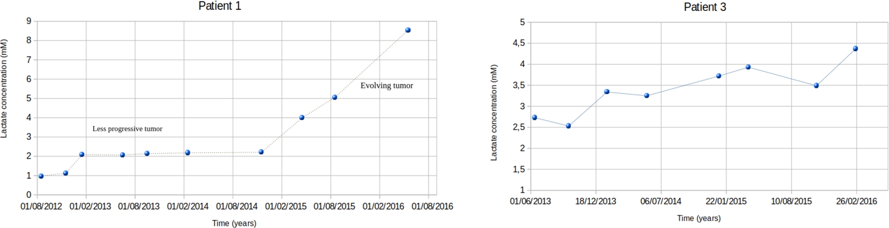
In this paragraph, our goal is to identify the parameters J, κ, $κ^{'}$ of equation (5.2). To this end, we use six in vivo data, collected by Magnetic Resonance Imaging (MRI) at the University Hospital of Poitiers, and corresponding to six anonymous patients suffering from glioma. For instance, Fig. 1 displays the lactate trajectories over the years, for patient 1 and patient 3.

Since we only have global data, we first assume that the lactate concentration is spatially constant in the brain. Hence equation (2.1) (with $ω = 0$ ) reduces to $\begin{array}{rcl} (5.1) & \partial_{t} φ + \frac{κ φ}{κ^{'} + | φ |} = J . \end{array}$ The identification is done using a descent algorithm based on (5.1) and its associated adjoint equation (see Section 5.2 for details).

Let us first focus on the parameters identification for patient 1. We can notice that the evolution of the lactates can be split into two phases: a first phase with almost constant lactates, corresponding to a slow tumor evolution and a second phase where the lactates evolve sharply, corresponding to a rapid tumor growth. Recalling that κ and J are tumor dependent, we proceed in the following way:

Fig. 1.

MRI data of glioma.

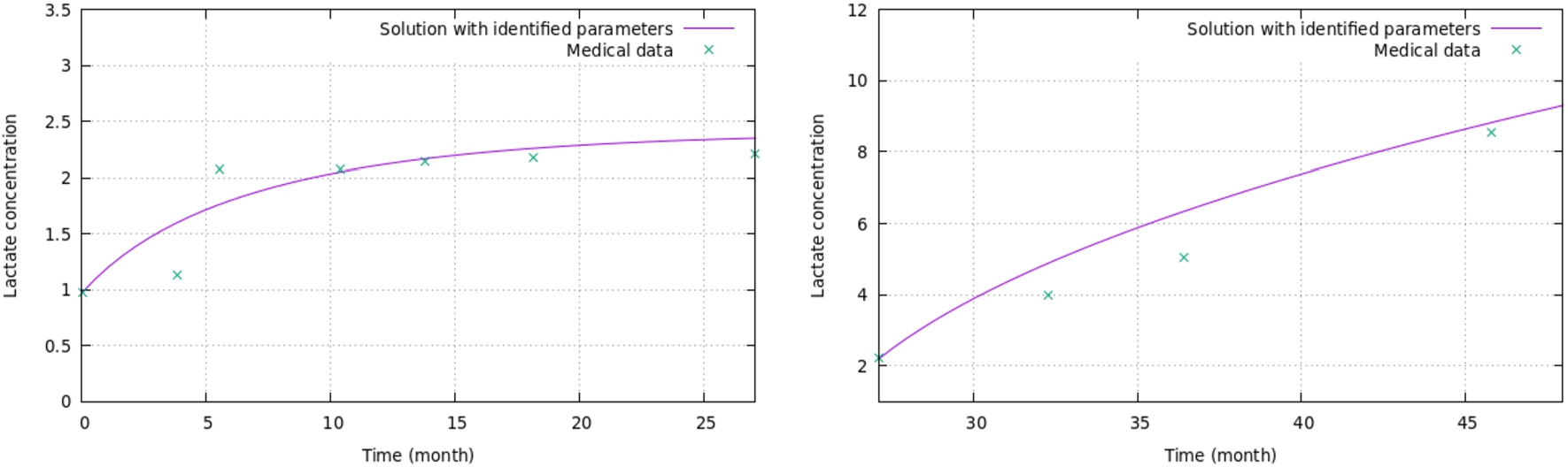
We identify κ, $κ^{'}$ and J, using the data corresponding to the first phase (slow evolution). We obtain $J_{1} = 0.726$ mM/month, $κ_{1} = 1, 122$ mM/month and $κ^{'} = 1.31$ mM. Then, we keep $κ^{'} = 1.31$ mM and identify $J_{2}$ and $κ_{2}$ , from the data of the second phase (see Fig. 2 and Table 1).

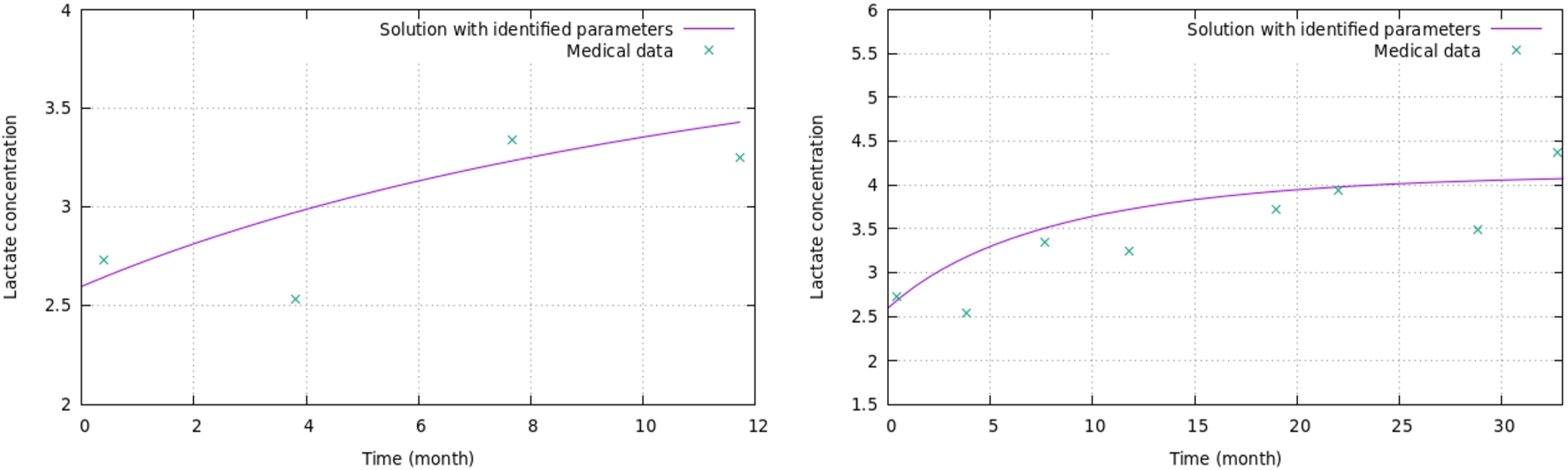
We proceed in a slightly different way for patients whose lactate trajectories can not be split into two phases (patient 3 for example). In this case we identify $κ_{1}$ , $κ^{'}$ and $J_{1}$ using the first points of the graph, then fix $κ^{'}$ and identify $κ_{2}$ and $J_{2}$ with the whole set of points (see Fig. 3). Table 1 displays the parameters $J_{1}$ , $κ_{1}$ , $κ^{'}$ , $J_{2}$ , $k_{2}$ for each of the six patients. Figure 2 and 3 display, for patients 1 and 3, the reconstructed lactate trajectories obtained thanks to the identified parameters.

Fig. 2.

Approximated lactate trajectory with identified parameters for patient 1. On the left, the phase with low variations. On the right the phase with larger variations.

Table 1

Parameters values of each patient

Patient	$J_{1}$ ( $mM/month$ )	$κ_{1}$ ( $mM/month$ )	$J_{2}$ ( $mM/month$ )	$κ_{2}$ ( $mM/month$ )	$κ^{'}$ ( $mM$ )
1	0.726	1.122	2.05	2.097	1.31
2	0.5477	1.442	1.55	2.721	5.582
3	2.034	2.292	3.44	3.87	0.515
4	0.203	1.074	1.194	2.729	6.599
5	0.34	1.34	0.385	1.515	10.564
6	0.106	1.144	0.355	1.725	7.724

Fig. 3.

Approximated lactate trajectory with identified parameters for patient 3. On the left, the phase with low variations, on the right the whole lactate trajectory.

5.2. Treatment optimization

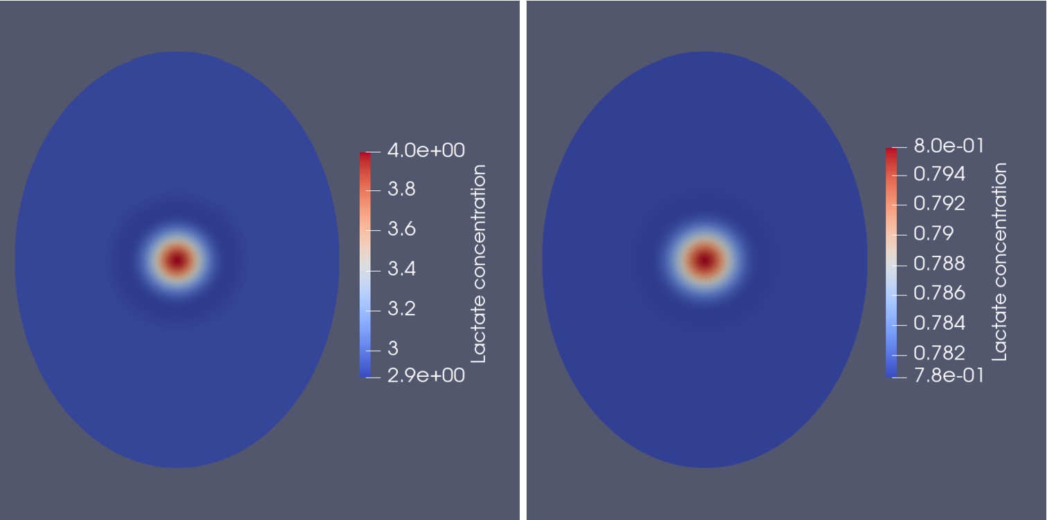
For the numerical simulations presented below, Ω is an ellipse parametrized by $x = 6 cos θ$ and $y = 8 sin θ$ , with $θ \in [0, 2 π]$ representing the part of the brain surrounding the tumor. Inside the ellipse, the initial tumor area is delimited by a circle of radius $r = 0.8$ . The target value of the lactate concentration is taken as $\hat{φ} = 0.8$ mM everywhere in the brain, corresponding to normal levels of intracellular lactate concentration.

In this section the control parameter ω is associated with J, meaning that the treatment has an impact on the production and consumption of the lactates (see Remark 2). Then, the equation for lactate reads: $\begin{matrix} (5.2) & \partial_{t} φ + α Δ^{2} φ - Δ f (φ) + \frac{κ φ}{κ^{'} + | φ |} = (1 - ω) J . \end{matrix}$ Here we assume that ω is constant (with respect to time and space) and that the duration of the treatment is fixed. Hence the functional reduces to: $\begin{array}{rcl} \tilde{J} (φ, ω) = \frac{1}{2} \int_{0}^{T} \int_{Ω} {(φ - \hat{φ})}^{2} d x d t + \frac{1}{2} \int_{Ω} {(φ (T) - \hat{φ} (T))}^{2} d x + \frac{1}{2} ω^{2} \end{array}$ For the simulations, we set $T = 6$ months, $\hat{φ} (x, t) = 0.8$ mM $\forall x \in Ω$ , $\forall t \in [0, T]$ . The algorithm is summarized on Algorithm 1.

Algorithm 1

Descent optimization algorithm

We use a finite element method for the space discretization of equation (5.2) and its associated adjoint equation, and a Crank–Nicolson scheme for the time discretization.

For each patient, we choose the parameters $κ^{'}$ , $κ_{2}$ and $J_{2}$ computed in the previous paragraph and recapitulated in Table 1.

For all of them, we take $φ_{0} = 0.8$ mM outside the tumor area, which corresponds to a normal lactate concentration. Inside the tumor area, we take for $φ_{0}$ the maximum lactate value reached by the patient before treatment. For instance, we take $φ_{0} = 8.56$ mM for patient 1 (see Fig. 1(a) at $t = 45.8$ months). After computations, we get $ω^{*} = 0.804$ . For patient 3, we take $φ_{0} = 4.37$ mM (see Fig. 1(b) at $t = 33$ months) and get $ω^{*} = 0.322$ . Table 2 shows the optimal dose of treatment and the value of $(1 - ω^{*}) J_{2}$ after treatment for every patients. In most cases, this latter value which is expected to be closed to the “normal” value of J, is indeed smaller than $J_{1}$ .

Table 2

Optimal treatment dose for all patients

Patient	optimal treatment $ω^{*}$	(1- $ω^{*}$ ) $J_{2}$ ( $mM/month$ )	$J_{1}$ ( $mM/month$ )
1	0.804	0.4018	0.726
2	0.856	0.2232	0.5477
3	0.322	2.3323	2.034
4	0.867	0.1588	0.203
5	0.744	0.0985	0.34
6	0.828	0.0610	0.106

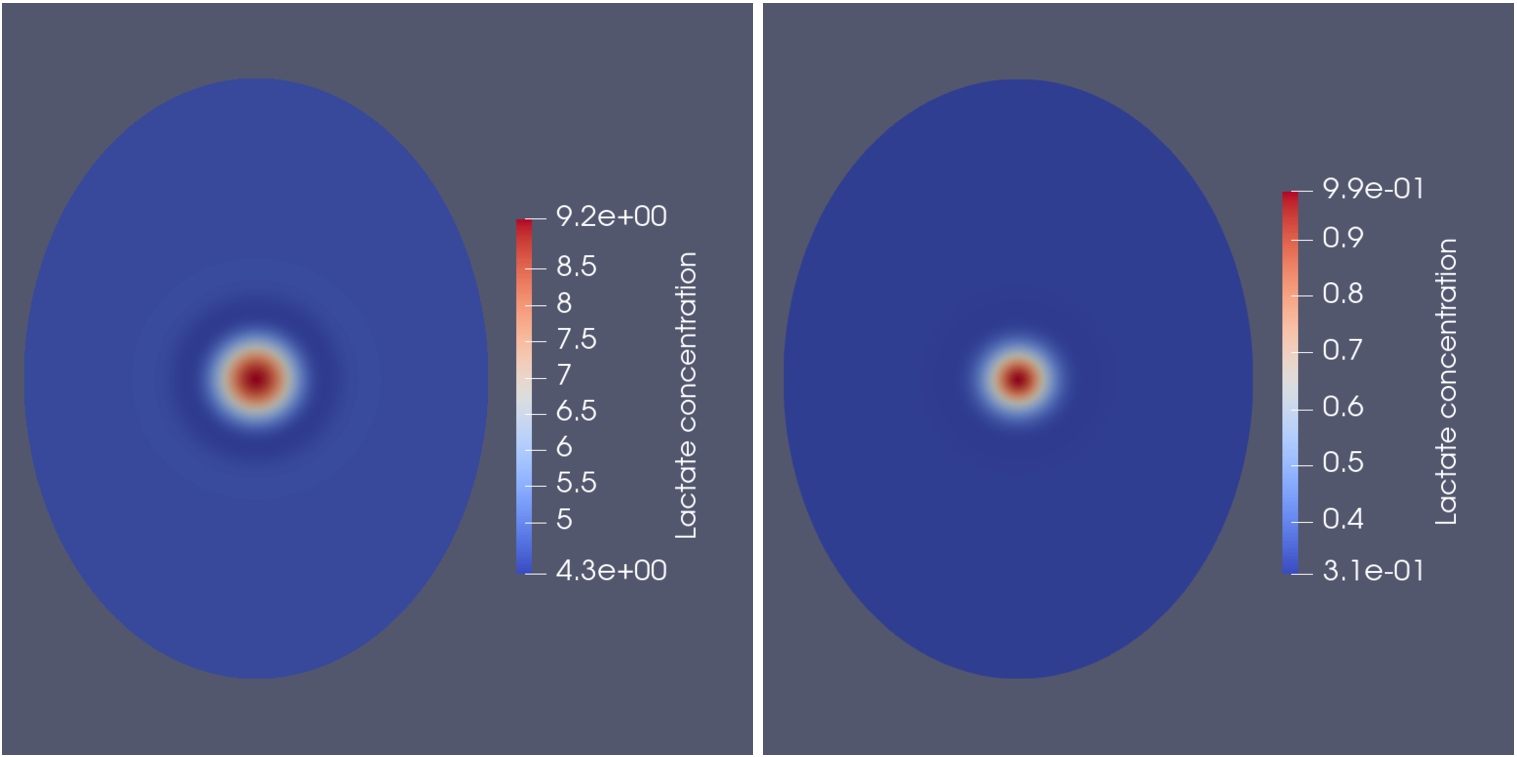
Figure 4 displays the final simulated lactate concentrations for patient 1, after 6 months, without treatment (left) and with the optimal treatment $ω^{*} = 0.804$ (right). Figure 5 displays the final lactate concentrations for patient 3, after 6 months, without treatment (left) and with the optimal treatment $ω^{*} = 0.322$ (right). These figures show that the treatment makes it possible to drastically reduce the concentration of lactate in the area of the tumor.

Fig. 4.

Spatial distribution of lactate levels at $T = 6$ months for patient 1. On the left, the patient didn’t get treatment. On the right the patient has undergone the optimal treatment.

Fig. 5.

Spatial distribution of lactate levels at $T = 6$ months for patient 3. On the left, the patient didn’t get treatment. On the right the patient has undergone the optimal treatment.

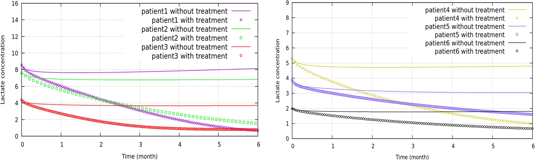
In Fig. 6 we compare, for every patient, the temporal evolution of their average values of lactate concentration in the tumor area, with and without treatment. The lactate levels stagnate without treatment, while, as expected, they decrease under the effect of the optimal treatment, until they reach (or get close to) the desired targets after six months.

Fig. 6.

Temporal evolution of lactate levels in the tumor area.

Footnotes

Derivation of the adjoint system

In order to derive the adjoint system, we apply the Lagrangian principle, defining the Lagrangian function with Lagrange multipliers ξ and π by: $\begin{array}{l} L (φ, μ, ω, τ, ξ, π) \\ = J_{r} (φ, ω, τ) - \int_{0}^{τ} \int_{Ω} (\partial_{t} φ - Δ μ + (1 - ω) g (φ) - J) ξ d x d t \\ - \int_{0}^{τ} \int_{Ω} (μ + α Δ φ - f (φ)) π d x d t \\ = J_{r} (φ, ω, τ) - \int_{0}^{τ} [- \int_{Ω} \partial_{t} ξ φ d x + \int_{Ω} \nabla μ \nabla ξ d x + \int_{Ω} (1 - ω) g (φ) ξ d x - \int_{Ω} J ξ d x] d t \\ - \int_{Ω} [ξ (τ) φ (τ) - ξ (0) φ (0)] d x - \int_{0}^{τ} [\int_{Ω} μ π d x - α \int_{Ω} \nabla φ \nabla π d x - \int_{Ω} f (φ) π d x] d t \end{array}$ The adjoint system is obtained by: $\begin{matrix} D_{φ} L (φ^{*}, μ^{*}, ω^{*}, τ^{*}, ξ, π) δ φ + D_{μ} L (φ^{*}, μ^{*}, ω^{*}, τ^{*}, ξ, π) δ μ = 0 \end{matrix}$ with $\begin{array}{l} D_{φ} L (φ^{*}, μ^{*}, ω^{*}, τ^{*}, ξ, π) δ φ \\ = \int_{0}^{τ^{*}} \int_{Ω} (φ^{*} - \hat{φ}) δ φ d x d t + \frac{1}{r} \int_{τ^{*} - r}^{τ^{*}} \int_{Ω} (φ^{*} - \hat{φ}) δ φ d x d t \\ + \int_{0}^{τ^{*}} \int_{Ω} \partial_{t} ξ δ φ d x d t - \int_{0}^{τ^{*}} \int_{Ω} (1 - ω^{*}) g^{'} (φ) ξ δ φ d x d t - \int_{0}^{τ^{*}} \int_{Ω} α Δ π δ φ d x d t \\ + \int_{0}^{τ^{*}} \int_{Γ} α \frac{\partial π}{\partial ν} δ φ d σ d t + \int_{0}^{τ^{*}} \int_{Ω} f^{'} (φ^{*}) π δ φ d x d t \\ - \int_{Ω} ξ (τ^{*}) δ φ (τ^{*}) d x + \int_{Ω} ξ (0) δ φ (0) d x \end{array}$ and $\begin{array}{l} D_{μ} L (φ^{*}, μ^{*}, ω^{*}, τ^{*}, ξ, π) δ μ \\ = \int_{0}^{τ^{*}} \int_{Ω} Δ ξ δ μ d x d t - \int_{0}^{τ^{*}} \int_{Γ} \frac{\partial ξ}{\partial ν} δ μ d σ d t - \int_{0}^{τ^{*}} \int_{Ω} π δ μ d x d t . \end{array}$

So the adjoint system reads $\begin{array}{l} - \partial_{t} ξ + α Δ π = f^{'} (φ^{*}) π - (1 - ω^{*}) g^{'} (φ^{*}) ξ + (φ^{*} - \hat{φ}) \\ + \frac{1}{r} (χ_{[τ^{*} - r, τ^{*}]} (t) (φ^{*} - \hat{φ})) on (0, τ^{*}) \times Ω \\ π = Δ ξ on (0, τ^{*}) \times Ω \\ \partial_{ν} ξ = \partial_{ν} π = 0 on (0, τ^{*}) \times Γ \\ ξ (τ^{*}) = 0 in Ω \end{array}$

References

Alsayed ,

Fakih ,

Miranville and

Wehbe , On an optimal control problem describing lactate production inhibition, Applicable Analysis (2022). doi:10.1080/00036811.2021.1999418.

Alsayed ,

Fakih ,

Miranville and

Wehbe , On an optimal control problem describing lactate transport inhibition, 2022, HAL-03850509.

Aubert ,

Costalat ,

P.J.

Magistretti and

Pellerin , Brain lactate kinetics: Modeling evidence for neuronal lactate uptake upon activation, Proceedings of the National Academy of Sciences of the United States of America 102 (2005), 16448–16453. doi:10.1073/pnas.0505427102.

Bonnans ,

J.-C.

Gilbert ,

Lemaréchal and

Sagastizábal , Optimisation Numérique: Aspects théoriques et pratiques (Mathématiques et Applications), Springer, 1997.

Cherfils ,

Gatti ,

Guillevin ,

Miranville and

Guillevin , On a tumor growth model with brain lactate kinetics, Mathematical Medecine and Biology 39(4) (2022), 382–409. doi:10.1093/imammb/dqac010.

Cherfils ,

Gatti ,

Miranville and

Guillevin , Analysis of a model for tumor growth and lactate exchanges in a glioma, DCDS-S 14(8) (2021), 2729–2749. doi:10.3934/dcdss.2020457.

Cloutier ,

F.B.

Bolger ,

J.P.

Lowry and

Wellstead , An integrative dynamic model of brain energy metabolism using in vivo neurochemical measurements, Journal of Computational Neuroscience 27 (2009), 391–414.

Colli ,

Gomez ,

Lorenzi ,

Marinoschi ,

Reali and

Rocca , Optimal control of cytotoxic and antiangiogenic therapies on prostate cancer growth, Maths. Models Method Appl. Sci. 31(7) (2021), 1419–1468. doi:10.1142/S0218202521500299.

Conti ,

Gatti and

Miranville , Mathematical analysis of a phase-field model of brain cancers with chemotherapy and antiangiogenic therapy effects, AIMS Mathematics 7(1) (2022), 1536–1561. doi:10.3934/math.2022090.

10.

Garcke ,

K.F.

Lam and

Rocca , Optimal control of treatment time in a diffuse interface model of tumor growth, Appl Math Optim 78 (2018), 495–544.

11.

C.E.

Griguer ,

C.R.

Oliva and

G.Y.

Gillespie , Glucose metabolism heterogeneity in human and mouse malignant glioma cell lines, Journal of Neuro-oncology 74 (2005), 123–133. doi:10.1007/s11060-004-6404-6.

12.

Guillevin ,

Miranville and

Perillat-Mercerot , Analysis of a mathematical model for brain lactate kinetics, Mathematical Biosciences and Engineering 15(5) (2018), 1225–1242. doi:10.3934/mbe.2018056.

13.

Guillevin ,

Menuel ,

J.-N.

Vallée ,

J.-P.

Françoise ,

Capelle ,

Habas ,

De Marco ,

Chiras and

Costalat , Mathematical modeling of energy metabolism and hemodynamics of WHO grade II gliomas using in vivo MR data, Comptes rendus biologies 334 (2011), 31–38.

14.

Jacquet and

Stéphanou , Metabolic reprogramming, questioning, and implications for cancer, Biology 10 (2021), 129. doi:10.3390/biology10020129.

15.

Lahutte-Auboin ,

Costalat ,

J.-P.

Françoise and

Guillevin , Dip and Buffering in a fast-slow system associated to Brain Lactacte Kinetics, preprint, arXiv:1308.0486.

16.

Lahutte-Auboin ,

Guillevin ,

J.-P.

Françoise ,

J.-N.

Vallée and

Costalat , On a minimal model for hemodynamics and metabolism of lactate: Application to low grade glioma and therapeutic strategies, Acta Biotheoretica 61 (2013), 79–89.

17.

Li ,

Miranville and

Guillevin , Cahn–Hilliard models for glial cells, Appl Math Optim 84 (2021), 1821–1842.

18.

P.J.

Magistretti and

Allaman , A cellular perspective on brain energy metabolism and functional imaging, Neuron 86 (2015), 883–901. doi:10.1016/j.neuron.2015.03.035.

19.

Mangia ,

Garreffa ,

Bianciardi ,

Giove ,

Di Salle and

Maraviglia , The aerobic brain: Lactate decrease at the onset of neural activity, Neuroscience 118 (2003), 7–10. doi:10.1016/S0306-4522(02)00792-3.

20.

J.R.

Mangiardi and

Yodice , Metabolism of the malignant astrocytoma, Neurosurgery 26 (1990), 1–19. doi:10.1227/00006123-199001000-00001.

21.

Miranville , The Cahn-Hilliard Equation: Recent Advances and Applications, Society for Industrial and Applied Mathematics, 2019.

22.

Signori , Optimal distributed control of an extended model of tumor growth with logarithmic potential, Appl Math Optim 82 (2020), 517–549. doi:10.1007/s00245-018-9538-1.

23.

Signori , Penalisation of Long Treatment Time and Optimal Control of a Tumour Growth Model of Cahn–Hilliard Type with Singular Potential, 23 May 2020, arXiv:1906.03460v2 [math.AP].

24.

Sonveaux

et al., Targeting lactate-fueled respiration selectively kills hypoxic tumor cells in mice, J. Clim. Invest. 118(12) (2008), 3930–3942.