Polynomial stabilization for thermoelastic Reissner–Mindlin–Timoshenko plates with structural damping

Abstract

In this paper, we are interested in studying the well-posedness, optimal polynomial stability, and the lack of exponential stability for a class of thermoelastic system of Reissner–Mindlin–Timoshenko plates with structural damping, that is, with the dissipation of Kelvin–Voigt type on the equations for the rotation angles. We also consider the thermal effect with thermal variables described by Fourier’s law of heat conduction.

Keywords

35B40 35L51 74D05 74F05

1. Introduction

The aim of this paper is to prove a result that characterizes polynomial stability for the a thermoelastic Reissner–Mindlin–Timoshenko plates with structural damping given by $\begin{array}{l} (1.1) & ρ_{1} ω_{t t} - K {(ω_{x} + ψ)}_{x} - K {(ω_{y} + φ)}_{y} = 0 in Ω \times R^{+}, \\ (1.2) & ρ_{2} ψ_{t t} - D L_{1} (ψ, φ) + K (ω_{x} + ψ) - γ L_{1} (ψ_{t}, φ_{t}) + β θ_{x} = 0 in Ω \times R^{+}, \\ (1.3) & ρ_{2} φ_{t t} - D L_{2} (ψ, φ) + K (ω_{y} + φ) - γ L_{2} (ψ_{t}, φ_{t}) + β θ_{y} = 0 in Ω \times R^{+}, \\ (1.4) & θ_{t} - κ Δ θ + β (ψ_{x t} + φ_{y t}) = 0 in Ω \times R^{+}, \end{array}$ where $\begin{array}{rcl} (1.5) & L_{1} (u, v) & : = & u_{x x} + (\frac{1 - μ}{2}) u_{y y} + (\frac{1 + μ}{2}) v_{x y} in Ω \times R^{+}, \\ (1.6) & L_{2} (u, v) & : = & v_{y y} + (\frac{1 - μ}{2}) v_{x x} + (\frac{1 + μ}{2}) u_{x y} in Ω \times R^{+} . \end{array}$ Here $ρ_{1} = ρ h$ , $ρ_{2} = \frac{ρ h^{3}}{12}$ where ρ is the (constant) mass per unit of surface area, h is the (uniform) plate thickness, μ is Poisson’s ratio ( $0 < μ < 1 / 2$ ), $D = \frac{E h^{3}}{12 (1 - μ^{2})}$ is the modulus of flexural rigidity, $K = \frac{k E h}{2 (1 + μ)}$ is the shear modulus where E is the Young’s modulus and k is the shear correction. Moreover, the functions ω, ψ and φ depend on $(x, y, t) \in Ω \times R^{+}$ and denote the transverse displacement of the plate and the rotational angles of a filament of the plate, respectively. More precise details will be given below about the derivation of our hyperbolic system. In the undamped case, in opposite to the 1-dimensional case, two rotational angles equations as well as the transverse displacement equation of a filament of the elastic structure are included in the mathematical modelling.

The initial data is given by $\begin{array}{l} (1.7) & ω (x, y, 0) = ω_{0} (x, y), ω_{t} (x, y, 0) = ω_{1} (x, y) in Ω, \\ (1.8) & ψ (x, y, 0) = ψ_{0} (x, y), ψ_{t} (x, y, 0) = ψ_{1} (x, y) in Ω, \\ (1.9) & φ (x, y, 0) = φ_{0} (x, y), φ_{t} (x, y, 0) = φ_{1} (x, y) in Ω, \\ (1.10) & θ (x, y, 0) = θ_{0} (x, y) in Ω, \end{array}$ where $Ω \subset R^{2}$ is a bounded domain with boundary $Γ = {\overline{Γ}}_{1} \cup {\overline{Γ}}_{2}$ , where $Γ_{1}$ and $Γ_{2}$ are non–empty. We will adopt the following boundary conditions provide in [7] $\begin{array}{l} (1.11) & w = θ = 0 on Γ \times R^{+}, \\ (1.12) & K (w_{x} + ψ, w_{y} + φ) \cdot n = 0 on Γ \times R^{+}, \\ (1.13) & φ = 0, (ψ_{x} + μ φ_{y}, \frac{1 - μ}{2} (φ_{x} + ψ_{y})) \cdot n = 0 on Γ_{1} \times R^{+}, \\ (1.14) & ψ = 0, (\frac{1 - μ}{2} (φ_{x} + ψ_{y}), φ_{y} + μ ψ_{x}) \cdot n = 0 on Γ_{2} \times R^{+}, \end{array}$ and in this work, $Ω \subset R^{2}$ is the rectangular region with the configuration given by $\begin{matrix} (1.15) & Ω : = [0, l_{1}] \times [0, l_{2}] with l_{1}, l_{2} > 0, \end{matrix}$ with boundary given by $\begin{array}{l} (1.16) & Γ_{1} & : = {(0, y) : 0 < y < l_{2}} \cup {(l_{1}, y) : 0 < y < l_{2}}, \\ (1.17) & Γ_{2} & : = {(x, 0) : 0 < x < l_{1}} \cup {(x, l_{2}) : 0 < x < l_{1}}, \end{array}$ satisfying $Γ : = {\overline{Γ}}_{1} \cup {\overline{Γ}}_{2}$ . We adopt the boundary conditions imposed in (1.11)–(1.14), viz: $\begin{array}{l} (1.18) & w = θ = 0 on Γ \times R^{+}, \\ (1.19) & φ = 0, w_{y} + φ = 0, ψ_{x} + μ φ_{y} = 0 on Γ_{1} \times R^{+}, \\ (1.20) & ψ = 0, w_{x} + ψ = 0, φ_{y} + μ ψ_{x} = 0 on Γ_{2} \times R^{+}, \end{array}$ considering $n = (1, 0)$ on $Γ_{1}$ and $n = (0, 1)$ on $Γ_{2}$ .

The Mindlin–Timoshenko model describes the elastic motion of a thin, homogeneous, isotropic plate. The motion is assumed to be elastic, in the sense that no permanent deformation of the plate occurs, see [4]. This model is considered one of the most important because it takes into account both transverse and rotational deformations. This model is used, for example, to model aircraft wings; see, for instance, [6].

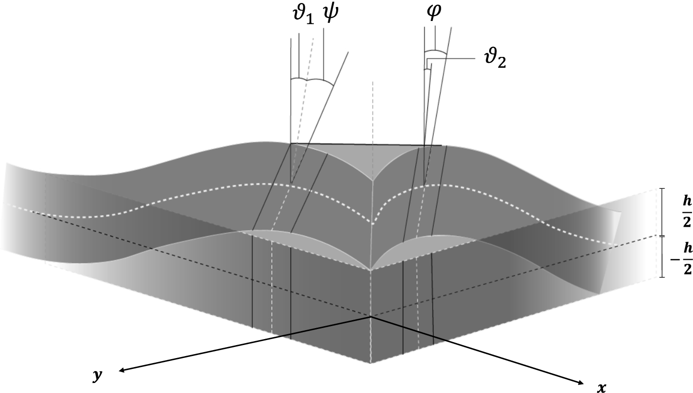
Consider a plate in rectangular coordinates $(x, y, z) \in R^{3}$ , where $Ω \subset R^{2}$ is a bounded domain with a smooth boundary, given as follows $Γ = \partial Ω$ . Here, we take into account the thickness of the plate h and we assume that, in a state of equilibrium, it occupies the region $R = Ω \times (- h / 2, h / 2)$ , that is, the faces are in the plane $z = h / 2$ , called the midplane of the plate (see Fig. 1). The functions $ψ (x, y, t)$ and $φ (x, y, t)$ represent the angles of rotation of a filament of the plate and the function $ω (x, y, t)$ represents the transverse displacement of the average surface of the plate, for $(x, y) \in Ω$ , $t > 0$ .

Fig. 1.

A deformed Mindlin–Timoshenko plate. We denote $ϑ_{1} : = - \frac{\partial w}{\partial x}$ the bending rotation in the x direction and $ϑ_{2} : = - \frac{\partial w}{\partial y}$ the bending rotation in the y direction.

In the model of Mindlin–Timoshenko [14,15], the plate filaments remain normal to the midplane if they are not subjected to any strain stress, but these filaments do not necessarily remain perpendicular to the midplane of the plate under deformation (see Fig. 1). This occurs because the deformation of the cross section is considered, which leads us to the following approximate relations $\begin{matrix} ψ \approx - (\frac{\partial ω}{\partial x} + \tilde{ψ}) and φ \approx - (\frac{\partial ω}{\partial y} + \tilde{φ}), \end{matrix}$ where $\tilde{ψ}$ , $\tilde{φ}$ represent a correction factor due to clipping effect, that is, the angles of rotation of the cross sections $x =$ const., $y =$ const. containing the filament which, when the plate is in equilibrium, is perpendicular to the middle surface at the point $(x, y, 0)$ . With the previous descriptions, the linear version of Mindlin–Timoshenko system is $\begin{array}{l} ρ h ω_{t t} - K {(ω_{x} + ψ)}_{x} - K {(ω_{y} + φ)}_{y} = 0 in Q, \\ \frac{1}{12} ρ h^{3} ψ_{t t} - L_{1} (ψ, φ) + K (ω_{x} + ψ) = 0 in Q, \\ \frac{1}{12} ρ h^{3} φ_{t t} - L_{2} (ψ, φ) + K (ω_{y} + φ) = 0 in Q, \end{array}$ with appropriate boundary conditions which will be better described below, where $L_{1} (\cdot, \cdot)$ and $L_{2} (\cdot, \cdot)$ are defined in (1.5) and (1.6), respectively. For a non-linear version see [15], see also [1] where an important conjecture for the non-linear model was proved and some open problems are described including the existence of solutions.

There are quite a few works on this type of system: [15] studied its well-posedness and analyzed its asymptotic limit when the parameter k tends to infinity. [14] studied problems of existence, uniqueness and some other important properties as the asymptotic behavior in time when some damping effects are considered.

Among the works that consider the thermal effect. [9] studied the strong stabilization of models for the Reissner–Mindlin plate equations with second sound, more precisely, the model considered includes thermal effects described according to Cattaneo’s law of heat conduction instead of Fourier’s law in classical thermoelasticity. The authors considered two different models regarding the property of compactness or non-compactness of the resolvent of the respective generators of the semigroup. In accordance with the compactness or non-compactness of the resolvent operator, a different criterion for strong stability was implemented to achieve the strong stabilization of each model. In a continuation paper, in [11], was showed the strong stability of models involving the thermoelastic Mindlin–Timoshenko plate equations with second sound and without applying any mechanical damping mechanism, in that the plate configuration was a single plate, in radially symmetric domains. Further to this result, was established the non-exponential stability of the model for a particular configuration under mixed boundary conditions on the shear angle variables and Dirichlet boundary conditions on the displacement and thermal variables when the heat flux is described by Fourier’s law of heat conduction, that is, the flux condition $q = - κ \nabla θ$ , $q$ the flux vector, θ the temperature function, is used to describe the temperature distribution in the beam or plate. Also, was computed the rate of polynomial decay of weak solutions of the model in a radially symmetric region under Dirichlet boundary conditions. Also, the model present thermal variables and free boundary conditions on the shear angle variables. More specifically, the configuration studied was $Ω \subset R^{2}$ as in (1.15).

The PDE system studied was $\begin{matrix} (1.21) & \begin{array}{l} ρ h w_{t t} - K {(w_{x} + ψ)}_{x} - K {(w_{y} + φ)}_{y} = 0, \\ \frac{ρ h^{3}}{12} ψ_{t t} - D L_{1} (ψ, φ) + K (w_{x} + ψ) + α D (\frac{1 + μ}{2}) θ_{x} = 0, \\ \frac{ρ h^{3}}{12} φ_{t t} - D L_{2} (ψ, φ) + K (w_{y} + φ) + α D (\frac{1 + μ}{2}) θ_{y} = 0, \\ γ θ_{t} - κ Δ θ + α D (\frac{1 + μ}{2}) (ψ_{t x} + φ_{t y}) = 0, \end{array} \end{matrix}$ with the boundary conditions: $\begin{array}{l} ψ = 0, ((\frac{1 - μ}{2}) (ψ_{y} + φ_{x}), φ_{y} + μ ψ_{x}) \cdot n = 0 on Γ_{1}, \\ φ = 0, (ψ_{x} + μ φ_{y}, (\frac{1 - μ}{2}) (ψ_{y} + φ_{x})) \cdot n = 0 on Γ_{2}, \\ w = 0 on Γ, \\ θ = 0 on Γ, \end{array}$ which, with $n = (0, 1)$ on $Γ_{1}$ and $n = (1, 0)$ on $Γ_{2}$ , yield for the shear angle variables the mixed boundary conditions $\begin{array}{l} ψ = 0, φ_{y} + μ ψ_{x} = 0 on Γ_{1} \\ φ = 0, ψ_{x} + μ φ_{y} = 0 on Γ_{2} . \end{array}$

In [12], was studied the polynomial stabilization of a two-dimensional thermoelastic Mindlin–Timoshenko plate model with no mechanical damping, with Dirichlet boundary conditions on the elastic as well as the thermal variables. The work complements the earlier work in [11] on the polynomial stabilization of a Mindlin–Timoshenko model in a radially symmetric domain with Dirichlet boundary conditions, thermal variables and free boundary conditions on the shear angle variables as described above. In particular, was investigated the effect of the Dirichlet boundary conditions on all the variables on the polynomial decay rate of the model.

In [16], was considered the linear Reissner–Mindlin–Timosheko plate equations $\begin{matrix} (1.22) & \begin{array}{l} ρ_{1} w_{t t} - K {(w_{x} + ψ)}_{x} - K {(w_{y} + φ)}_{y} = 0, \\ ρ_{2} ψ_{t t} - D L_{1} (ψ, φ) + K (w_{x} + ψ) + γ θ_{x} = 0, \\ ρ_{2} φ_{t t} - D L_{2} (ψ, φ) + K (w_{y} + φ) + γ θ_{y} = 0, \\ ρ_{3} θ_{t} + κ div q + β θ + γ (ψ_{t x} + φ_{t y}) = 0, \\ τ_{0} q_{t} + δ q + κ \nabla θ = 0 . \end{array} \end{matrix}$ in a bounded domain. Firstly, using the semigroup theory was showed that the initial-boundary value problem (1.22) subject to corresponding initial conditions as well as homogeneous Dirichlet and Neumann boundary conditions on both elastic and thermal variables on different portions of the boundary is well-posed. Second, was proved the lack of strong stability for this problem provided Γ is smooth for a particular set of boundary conditions. Further was shown that mechanical damping for all three variables w, φ, and ψ leads to an exponential decay rate under Dirichlet boundary conditions for the elastic and Neumann boundary conditions for the thermal part of the system. Restricting the domain Ω and the data to the rotationally symmetric case, was proved that a single mechanical damping on w is enough to exponentially stabilize the system.

Among the works without the thermal effect. [10] handled a linear model for the magnetoelastic interactions in a two-dimensional electrically conducting Mindlin–Timoshenko plate. The unique solvability of the model was established within the framework of semigroup theory. Spectral analysis methods are used to show strong asymptotic stability and determine the polynomial decay rate of weak solutions.

In [18], the authors proved the asymptotic stability of Mindlin–Timoshenko plates with dissipation of Kelvin–Voigt type on the equations for the rotation angles, that is, the system $\begin{matrix} (1.23) & \begin{array}{l} ρ h w_{t t} - K {(w_{x} + ψ)}_{x} - K {(w_{y} + φ)}_{y} - D_{0} Δ w_{t} = 0 in Ω \times R^{+}, \\ \frac{ρ h^{3}}{12} ψ_{t t} - D L_{1} (ψ, φ) + K (w_{x} + ψ) - D_{1} L_{1} (ψ_{t}, φ_{t}) = 0 in Ω \times R^{+}, \\ \frac{ρ h^{3}}{12} φ_{t t} - D L_{2} (ψ, φ) + K (w_{y} + φ) - D_{1} L_{2} (ψ_{t}, φ_{t}) = 0 in Ω \times R^{+}, \end{array} \end{matrix}$ where Ω is a bounded domain of $R^{2}$ with Lipschitz boundary $Γ = \partial Ω$ , and $L_{1} (\cdot, \cdot)$ , $L_{2} (\cdot, \cdot)$ are defined in (1.5) and (1.6), respectively. This system models the vibrations of a thin plate with reference configuration Ω by taking into account the displacements and rotations caused by the movement. We notice that the damping terms $L_{1} (ψ_{t}, φ_{t})$ and $L_{2} (ψ_{t}, φ_{t})$ correspond to the called Kelvin–Voigt damping. Indeed, materials with Kelvin–Voigt damping are characterized by having stress proportional to strain and strain rate, see, for instance, [18] and references therein for more details.

To the system (1.23) was considered the initial conditions $\begin{array}{l} w (x, y, 0) = w_{0} (x, y), w_{t} (x, y, 0) = w_{1} (x, y) in Ω, \\ ψ (x, y, 0) = ψ_{0} (x, y), ψ_{t} (x, y, 0) = ψ_{1} (x, y) in Ω, \\ φ (x, y, 0) = φ_{0} (x, y), φ_{t} (x, y, 0) = φ_{1} (x, y) in Ω, \end{array}$ and two different types of boundary conditions: the Dirichlet condition $\begin{matrix} w = ψ = φ = 0 on Γ \times [0, \infty), \end{matrix}$ or a mixed condition $\begin{array}{l} w = 0 on Γ \times [0, \infty), \\ ψ = 0, (\frac{1 - μ}{2} (φ_{x} + ψ_{y}), φ_{y} + μ ψ_{x}) \cdot ν = 0 on Γ_{1} \times [0, \infty), \\ φ = 0, (ψ_{x} + μ φ_{y}, \frac{1 - μ}{2} (φ_{x} + ψ_{y})) \cdot ν = 0 on Γ_{2} \times [0, \infty), \end{array}$ where $Γ = {\bar{Γ}}_{1} \cup {\bar{Γ}}_{2}$ is a partition of Γ given by nonempty disjoint open sets $Γ_{1}$ , $Γ_{2}$ , and $ν = (ν_{1}, ν_{2})$ is the unit exterior normal to Γ. The authors in [18] proved that the corresponding evolution semigroup is analytic if a viscoelastic damping is also effective over the equation for the transversal displacements. On the contrary, if the transversal displacement is undamped, was shown that the semigroup is neither analytic nor exponentially stable. In addition, in the latter case, was shown that the solution decays polynomially and we prove that the decay rate found is optimal. It is noteworthy that the work [18] was the first to consider the Kelvin Voigt damping effect, proving analyticity and exponential decay with optimal rate.

More recently, we can consider [4] and [5]. In [4] was shown that there exists a critical number that stabilizes the Reissner–Mindlin–Timoshenko system with frictional dissipation acting only on the equation for the transverse displacement, more precisely, related to the system $\begin{array}{l} ρ_{1} ω_{t t} - K {(ω_{x} + ψ)}_{x} - K {(ω_{y} + φ)}_{y} + d_{1} ω_{t} = 0 in Ω \times R^{+}, \\ ρ_{2} ψ_{t t} - D L_{1} (ψ, φ) + K (ω_{x} + ψ) = 0 in Ω \times R^{+}, \\ ρ_{2} φ_{t t} - D L_{2} (ψ, φ) + K (ω_{y} + φ) = 0 in Ω \times R^{+} . \end{array}$ Recording that, $ρ_{1} = ρ h$ , $ρ_{2} = \frac{ρ h^{3}}{12}$ where ρ is the (constant) mass per unit of surface area, h is the (uniform) plate thickness, μ is Poisson’s ratio $(0 < μ < 1 / 2)$ , $D = \frac{E h^{3}}{12 (1 - μ^{2})}$ is the modulus of flexural rigidity, $K = \frac{k E h}{2 (1 + μ)}$ is the shear modulus where E is the Young’s modulus and k is the shear correction. The authors in [4] proved that the Reissner–Mindlin–Timoshenko system has two speed characteristics $v_{1}^{2} : = K / ρ_{1}$ and $v_{2}^{2} : = D / ρ_{2}$ and we show that the system is exponentially stable if, and only if, $\begin{matrix} (1.24) & v_{1}^{2} = v_{2}^{2} . \end{matrix}$ Moreover, they proved that the system is polynomially stable with optimal decay rate. Numerical experiments using finite differences where given to confirm the analytical results.

In [5], the authors proved that the critical number that stabilizes the Reissner–Mindlin–Timoshenko system still holds, now adding the frictional dissipation acting on rotation angles, that is, the system $\begin{array}{l} ρ_{1} ω_{t t} - K {(ω_{x} + ψ)}_{x} - K {(ω_{y} + φ)}_{y} = 0, \\ ρ_{2} ψ_{t t} - D L_{1} (ψ, φ) + K (ω_{x} + ψ) + d_{1} ψ_{t} = 0, \\ ρ_{2} φ_{t t} - D L_{2} (ψ, φ) + K (ω_{y} + φ) + d_{2} φ_{t} = 0, \end{array}$ and they showed that the system is exponentially stable if and only if (1.24) holds. Moreover, for $v_{1}^{2} \neq v_{2}^{2}$ , was proved that the system is polynomially stable and determined an optimal estimate for the decay. To confirm the analytical results, was computed the numerical solutions by means of several numerical experiments by using a finite difference method. It is worth noting that the works [4] and [5] were the first to prove the exponential decay depending on the known relationship of equality between the speeds.

Also more recently, in notorious paper [1], the authors showed how the so-called von Kármán model (the model obtained when one assumes the filament of the plate to remain orthogonal to the deformed middle surface and the transverse shear effects are neglected; see [15]) can be obtained as a singular limit of a Mindlin–Timoshenko system when the modulus of elasticity in shear K tends to infinity. The result gave a positive answer to a conjecture by Lagnese and Lions in 1988. Introducing damping mechanisms, they also obtained that the energy of solutions for this modified Mindlin–Timoshenko system decays exponentially, uniformly with respect to the parameter K. As $K \to \infty$ , they obtained the damped von Kármán model with associated energy exponentially decaying to zero as well. It is noteworthy that the model of Mindlin–Timoshenko studied in [1] was a complete and non-linear model as described in [15]. For more details see, for instance, [1] and the reference therein.

The paper is organized as follows. In Section 2, we discuss two theorems as main tools related to exponential stability and polynomial stability. In Section 3, we will show the well-posedness of the system (1.1)–(1.4) using the semigroup techniques. In Section 4, we will prove the lack of exponential decay to the system (1.1)–(1.4). Section 5, is concerned with the polynomial decay and its optimal estimate to the system.

2. Main tools

Concerning the mathematical analysis, the method that we use to determine the asymptotic behaviour is based on Gearhart–Herbst–Prüss–Huang Theorem for dissipative systems [13,17].

Theorem 2.1.
Let $S (t) = e^{A t}$ be a $C_{0}$ -semigroup of contractions on a Hilbert space $H$ . Then $S (t)$ is exponentially stable if and only if $\begin{array}{l} (2.1) & i R \equiv {i λ : λ \in R} \subset ϱ (A) \end{array}$ and $\begin{array}{l} (2.2) & \underset{| λ | \to \infty}{lim^{‾}} {‖ {(i λ I - A)}^{- 1} ‖}_{L (H)} < \infty, \end{array}$ hold, where $ϱ (A)$ is the resolvent set of the differential operator $A$ .

On the other hand, to show the polynomial stability and the optimality of its rate we use the result due to Borichev & Tomilov (see [2], Theorem 2.4). Theorem 2.2.
Let $S (t) = e^{A t}$ be a contraction semigroup on a complex Hilbert space $H$ . Suppose that $i R \subset ϱ (A)$ . Then, for every fixed $α > 0$ , $\begin{matrix} {‖ {(i λ I - A)}^{- 1} ‖}_{L (H)} = O (| λ |^{α}) as | λ | \to \infty \end{matrix}$ if and only if $\begin{matrix} {‖ S (t) A^{- 1} ‖}_{L (H)} = O (t^{- 1 / α}) as t \to \infty . \end{matrix}$

3. Semigroup setting and existence result

In this section, we will show that the system (1.1)–(1.4) is well posed using the semigroup techniques. Let us denote by $\begin{array}{l} (3.1) & H : = H_{0}^{1} (Ω) \times L^{2} (Ω) \times H_{Γ_{1}}^{1} (Ω) \times L^{2} (Ω) \times H_{Γ_{2}}^{1} (Ω) \times L^{2} (Ω) \times H_{0}^{1} (Ω), \end{array}$ the Hilbert space with internal product given by $\begin{array}{l} {(U, V)}_{H} = & ρ_{1} \int_{Ω} W^{1} \overline{W^{2}} d x d y + ρ_{2} \int_{Ω} Ψ^{1} \overline{Ψ^{2}} d x d y + ρ_{2} \int_{Ω} Φ^{1} \overline{Φ^{2}} d x d y \\ + K \int_{Ω} (w_{x}^{1} + ψ^{1}) (\overline{w_{x}^{2} + ψ^{2}}) d x d y + K \int_{Ω} (w_{y}^{1} + φ^{1}) (\overline{w_{y}^{2} + φ^{2}}) d x d y \\ + D (1 - μ) \int_{Ω} ψ_{x}^{1} \overline{ψ_{x}^{2}} d x d y + D (1 - μ) \int_{Ω} φ_{y}^{1} \overline{φ_{y}^{2}} d x d y \\ + \frac{D (1 - μ)}{2} \int_{Ω} (ψ_{y}^{1} + φ_{x}^{1}) (\overline{ψ_{y}^{2} + φ_{x}^{2}}) d x d y \\ (3.2) & + D μ \int_{Ω} (ψ_{x}^{1} + φ_{y}^{1}) \overline{(ψ_{x}^{2} + φ_{y}^{2})} d x d y + \int_{Ω} θ^{1} \overline{θ^{2}} d x d y \end{array}$ and norm given by $\begin{array}{rcl} ‖ U ‖_{H}^{2} & = & {‖ {(w^{1}, W^{1}, ψ^{1}, Ψ^{1}, φ^{1}, Φ^{1}, θ^{1})}^{⊤} ‖}_{H}^{2} \\ = & ρ_{1} {‖ W^{1} ‖}^{2} + ρ_{2} {‖ Ψ^{1} ‖}^{2} + ρ_{2} {‖ Φ^{1} ‖}^{2} + K {‖ w_{x}^{1} + ψ^{1} ‖}^{2} + K {‖ w_{y}^{1} + φ^{1} ‖}^{2} \\ + D (1 - μ) {‖ ψ_{x}^{1} ‖}^{2} + D (1 - μ) {‖ φ_{y}^{1} ‖}^{2} + \frac{D (1 - μ)}{2} {‖ ψ_{y}^{1} + φ_{x}^{1} ‖}^{2} \\ + D μ {‖ ψ_{x}^{1} + φ_{y}^{1} ‖}^{2} + {‖ θ^{1} ‖}^{2}, \end{array}$ where $U = {(w^{1}, W^{1}, ψ^{1}, Ψ^{1}, φ^{1}, Φ^{1}, θ^{1})}^{⊤}$ , $V = {(w^{2}, W^{2}, ψ^{2}, Ψ^{2}, φ^{2}, Φ^{2}, θ^{2})}^{⊤}$ and $\begin{matrix} H_{Γ_{i}}^{1} (Ω) : = {f \in H^{1} (Ω) | f = 0 on Γ_{i}}, i = 1, 2 . \end{matrix}$

If we write $U = {(ω, ω_{t}, ψ, ψ_{t}, φ, φ_{t}, θ)}^{⊤}$ and $U_{0} = {(ω_{0}, ω_{1}, ψ_{0}, ψ_{1}, φ_{0}, φ_{1}, θ_{0})}^{⊤}$ then the equations (1.1)–(1.4) can be rewritten as follows $\begin{array}{l} (3.3) & \frac{d U (t)}{d t} = A U (t), for t > 0, \\ (3.4) & U (0) = U_{0}, \end{array}$ where $A : D (A) \subset H \to H$ is the operator defined formally by $\begin{array}{l} A : = (\begin{matrix} 0 & I_{d} (\cdot) & 0 & 0 & 0 & 0 & 0 \\ \frac{K}{ρ_{1}} Δ (\cdot) & 0 & \frac{K}{ρ_{1}} \partial_{x} (\cdot) & 0 & \frac{K}{ρ_{1}} \partial_{y} (\cdot) & 0 & 0 \\ 0 & 0 & 0 & I_{d} (\cdot) & 0 & 0 & 0 \\ - \frac{K}{ρ_{2}} \partial_{x} (\cdot) & 0 & B_{1} (\cdot) & {\tilde{B}}_{1} (\cdot) & \frac{D}{ρ_{2}} (\frac{1 + μ}{2}) \partial_{x y}^{2} (\cdot) & \frac{γ}{ρ_{2}} (\frac{1 + μ}{2}) \partial_{x y}^{2} (\cdot) & - \frac{β}{ρ_{2}} \partial_{x} (\cdot) \\ 0 & 0 & 0 & 0 & 0 & I_{d} (\cdot) & 0 \\ - \frac{K}{ρ_{2}} \partial_{y} (\cdot) & 0 & \frac{D}{ρ_{2}} (\frac{1 + μ}{2}) \partial_{x y}^{2} (\cdot) & \frac{γ}{ρ_{2}} (\frac{1 + μ}{2}) \partial_{x y}^{2} (\cdot) & B_{2} (\cdot) & {\tilde{B}}_{2} (\cdot) & - \frac{β}{ρ_{2}} \partial_{y} (\cdot) \\ 0 & 0 & 0 & - β \partial_{x} (\cdot) & 0 & - β \partial_{y} (\cdot) & κ Δ (\cdot) \end{matrix}), \end{array}$ where the operators $B_{i} (\cdot)$ and ${\tilde{B}}_{i} (\cdot)$ ( $i = 1, 2$ ) are given by $\begin{array}{l} B_{1} (\cdot) : = \frac{D}{ρ_{2}} [\partial_{x}^{2} (\cdot) + (\frac{1 - μ}{2}) \partial_{y}^{2} (\cdot)] - \frac{K}{ρ_{2}} I_{d} (\cdot), {\tilde{B}}_{1} (\cdot) : = \frac{γ}{ρ_{2}} [\partial_{x}^{2} (\cdot) + (\frac{1 - μ}{2}) \partial_{y}^{2} (\cdot)], \\ B_{2} (\cdot) : = \frac{D}{ρ_{2}} [(\frac{1 - μ}{2}) \partial_{x}^{2} (\cdot) + \partial_{y}^{2} (\cdot)] - \frac{K}{ρ_{2}} I_{d} (\cdot), {\tilde{B}}_{2} (\cdot) : = \frac{γ}{ρ_{2}} [(\frac{1 - μ}{2}) \partial_{x}^{2} (\cdot) + \partial_{y}^{2} (\cdot)], \end{array}$ $I_{d} (\cdot)$ is the identity operator and $\begin{array}{rcl} D (A) & = & \{U : = {(ω, W, ψ, Ψ, φ, Φ, θ)}^{⊤} \in H | \\ (3.5) & \begin{matrix} U satisfies (1.18)–(1.20), ω, θ \in H^{2} (Ω), W \in H_{0}^{1} (Ω), \\ Ψ \in H_{Γ_{1}}^{1} (Ω), D L_{1} (ψ, φ) + γ L_{1} (Ψ, Φ) \in L^{2} (Ω), \\ Φ \in H_{Γ_{2}}^{1} (Ω), D L_{2} (ψ, φ) + γ L_{2} (Ψ, Φ) \in L^{2} (Ω) . \end{matrix}\} . \end{array}$ Note that $D L_{1} (ψ, φ) + γ L_{1} (Ψ, Φ)$ , $D L_{2} (ψ, φ) + γ L_{2} (Ψ, Φ) \in L^{2} (Ω)$ gives more regularity to functions $(ψ, φ, Ψ, Φ)$ .

In the next theorem we assume that $Γ_{1}$ is non-empty, $\overline{Γ_{1}} \cap \overline{Γ_{2}}$ is empty and $\partial Ω$ is either $C^{2}$ or piecewise $C^{2}$ with all of the cusps being of angle of at least $π / 2$ [14].

Theorem 3.1.
The operator $A$ generates a C ₀ -semigroup $S (t)$ of contraction on $H$ . Thus, for any initial data $U_{0} \in H$ , the problem ( 1.1 )–( 1.4 ) has a unique mild solution $U \in C^{0} ([0, \infty), H)$ . Moreover, if $U_{0} \in D (A)$ , then U is a classical solution of ( 1.1 )–( 1.4 ), i.e., $U \in C^{1} ([0, \infty), H) \cap C^{0} ([0, \infty), D (A))$ .
Proof.
Firstly we note that $A$ is a dissipative operator in $H$ . Simple calculations give us $\begin{array}{l} Re {(A U, U)}_{H} = & - γ (1 - μ) (‖ Ψ_{x} ‖^{2} + ‖ Φ_{y} ‖^{2}) - γ μ ‖ Ψ_{x} + Φ_{y} ‖^{2} \\ (3.6) & - γ (\frac{1 - μ}{2}) ‖ Ψ_{y} + Φ_{x} ‖^{2} - κ ‖ \nabla θ ‖^{2} ⩽ 0, \end{array}$ from where it follows that $A$ is a dissipative operator. Next, to prove that $0 \in ϱ (A)$ (resolvent set of $A$ ), we let $F = {(f^{1}, f^{2}, f^{3}, f^{4}, f^{5}, f^{6}, f^{7})}^{⊤} \in H$ and we look for a unique $U = {(ω, W, ψ, Ψ, φ, Φ, θ)}^{⊤} \in D (A)$ such that $\begin{array}{rcl} (3.7) & - A U = F, \end{array}$ and $\begin{array}{rcl} (3.8) & ‖ U ‖_{H} ⩽ C ‖ F ‖_{H}, \end{array}$ for some $C > 0$ independent of F and U. Equivalently, we get $W = - f^{1}$ , $Ψ = - f^{3}$ , $Φ = - f^{5}$ and the following system $\begin{array}{l} (3.9) & - \frac{K}{ρ_{1}} {(ω_{x} + ψ)}_{x} - \frac{K}{ρ_{1}} {(ω_{y} + φ)}_{y} = f^{2}, \\ (3.10) & - \frac{D}{ρ_{2}} L_{1} (ψ, φ) + \frac{K}{ρ_{2}} (ω_{x} + ψ) + \frac{β}{ρ_{2}} θ_{x} = f^{4} - \frac{γ}{ρ_{2}} L_{1} (f^{3}, f^{5}), \\ (3.11) & - \frac{D}{ρ_{2}} L_{2} (ψ, φ) + \frac{K}{ρ_{2}} (ω_{y} + φ) + \frac{β}{ρ_{2}} θ_{y} = f^{6} - \frac{γ}{ρ_{2}} L_{2} (f^{3}, f^{5}), \\ (3.12) & - κ Δ θ = f^{7} + β (f_{x}^{3} + f_{y}^{5}) . \end{array}$ Multiplying (3.9)–(3.12) by ${\overline{ω}}^{}$ , ${\overline{ψ}}^{}$ , ${\overline{φ}}^{}$ , $σ {\overline{θ}}^{}$ ( $σ > 0$ ) respectively, integrating in Ω and taking the sum, we obtain the equivalent variational problem: $\begin{array}{rcl} (3.13) & B_{σ} ((ω, ψ, φ, θ), (ω^{}, ψ^{}, φ^{}, θ^{})) & = & Z_{σ} (ω^{}, ψ^{}, φ^{}, θ^{}), \end{array}$ where $B_{σ} (\cdot, \cdot)$ is the sesquilinear form in $H_{0}^{1} (Ω) \times H_{Γ_{1}}^{1} (Ω) \times H_{Γ_{2}}^{1} (Ω) \times H_{0}^{1} (Ω)$ given by $\begin{array}{l} B_{σ} ((ω, ψ, φ, θ), (ω^{}, ψ^{}, φ^{}, θ^{})) \\ (3.14) & : = K \int_{Ω} (ω_{x} + ψ) \overline{(ω_{x}^{} + ψ^{})} d x d y + K \int_{Ω} (ω_{y} + φ) \overline{(ω_{y}^{} + φ^{})} d x d y \\ + D (1 - μ) \int_{Ω} ψ_{x} {\overline{ψ}}_{x}^{} d x d y + D (1 - μ) \int_{Ω} φ_{y} {\overline{φ}}_{y}^{} d x d y \\ + D (\frac{1 - μ}{2}) \int_{Ω} (ψ_{y} + φ_{x}) \overline{(ψ_{y}^{} + φ_{x}^{})} d x d y \\ + D μ \int_{Ω} (ψ_{x} + φ_{y}) \overline{(ψ_{x}^{} + φ_{y}^{})} d x d y - β \int_{Ω} θ {\overline{ψ}}_{x}^{} d x d y \\ (3.15) & - β \int_{Ω} θ {\overline{φ}}_{y}^{} d x d y + σ κ \int_{Ω} \nabla θ \cdot \nabla {\overline{θ}}^{} d x d y, \end{array}$ and $Z_{σ} (\cdot, \cdot, \cdot, \cdot)$ is a continuous linear form in $H_{0}^{1} (Ω) \times H_{Γ_{1}}^{1} (Ω) \times H_{Γ_{2}}^{1} (Ω) \times H_{0}^{1} (Ω)$ given by $\begin{array}{rcl} Z_{σ} (ω^{}, ψ^{}, φ^{}, θ^{}) & : = & ρ_{1} \int_{Ω} f^{2} {\overline{ω}}^{} d x d y + ρ_{2} \int_{Ω} f^{4} {\overline{ψ}}^{} d x d y + ρ_{2} \int_{Ω} f^{6} {\overline{ψ}}^{} d x d y \\ + σ \int_{Ω} f^{7} {\overline{θ}}^{} d x d y + γ (1 - μ) \int_{Ω} f_{x}^{3} {\overline{ψ}}_{x}^{} d x d y \\ + γ (\frac{1 - μ}{2}) \int_{Ω} (f_{y}^{3} + f_{x}^{5}) \overline{(ψ_{y}^{} + φ_{x}^{})} d x d y \\ + γ μ \int_{Ω} (f_{x}^{3} + f_{y}^{5}) \overline{(ψ_{x}^{} + φ_{y}^{})} d x d y + γ (1 - μ) \int_{Ω} f_{y}^{5} {\overline{φ}}_{y}^{} d x d y \\ (3.16) & + σ β \int_{Ω} (f_{x}^{3} + f_{y}^{5}) {\overline{θ}}^{} d x d y . \end{array}$

The parameter $σ > 0$ is chosen large enough to ensure the coercivity. Since $\begin{array}{rcl} B_{σ} ((ω, ψ, φ, θ), (ω, ψ, φ, θ)) & : = & K ‖ ω_{x} + ψ ‖^{2} + K ‖ ω_{y} + φ ‖^{2} + D (1 - μ) ‖ ψ_{x} ‖^{2} \\ + D (1 - μ) ‖ φ_{y} ‖^{2} + D (\frac{1 - μ}{2}) ‖ ψ_{y} + φ_{x} ‖^{2} + D μ ‖ ψ_{x} + φ_{y} ‖^{2} \\ + σ κ ‖ \nabla θ ‖^{2} - β \int_{Ω} θ {\overline{ψ}}_{x} d x d y - β \int_{Ω} θ {\overline{φ}}_{y} d x d y, \end{array}$ the sesquilinear form $B_{σ} (\cdot, \cdot)$ is strongly coercive on $H_{0}^{1} (Ω) \times H_{Γ_{1}}^{1} (Ω) \times H_{Γ_{2}}^{1} (Ω) \times H_{0}^{1} (Ω)$ , and since (3.16) defines a continuous linear functional of $(ω^{}, ψ^{}, φ^{}, θ^{})$ , by Lax-Milgram’s Theorem, problem (3.13) admits a unique solution $(ω, ψ, φ, θ) \in H_{0}^{1} (Ω) \times H_{Γ_{1}}^{1} (Ω) \times H_{Γ_{2}}^{1} (Ω) \times H_{0}^{1} (Ω)$ . By taking test functions in the form $(ω_{1}, 0, 0, 0)$ , $(0, ψ_{1}, 0, 0)$ , $(0, 0, φ_{1}, 0)$ and $(0, 0, 0, θ_{1})$ with $ω_{1}, ψ_{1}, φ_{1}, θ_{1} \in D (Ω)$ (space of test functions), it is easy to see that $(ω, ψ, φ, θ)$ satisfies system (3.9)–(3.12) in the distributional sense. This also shows that $ω, θ \in H^{2} (Ω)$ and also $D L_{1} (ψ, φ) + γ L_{1} (Ψ, Φ), D L_{2} (ψ, φ) + γ L_{2} (Ψ, Φ) \in L^{2} (Ω)$ , because $\begin{array}{l} (3.17) & K (ω_{x x} + ω_{y y}) = - K (ψ_{x} + φ_{y}) - ρ_{1} f^{2} \in L^{2} (Ω), \\ (3.18) & D L_{1} (ψ, φ) + γ L_{1} (Ψ, Φ) = β θ_{x} + K (ω_{x} + ψ) - ρ_{2} f^{4} \in L^{2} (Ω), \\ (3.19) & D L_{2} (ψ, φ) + γ L_{2} (Ψ, Φ) = β θ_{y} + K (ω_{y} + φ) - ρ_{2} f^{6} \in L^{2} (Ω), \\ (3.20) & κ Δ θ = - β (f_{x}^{3} + f_{y}^{5}) - f^{7} \in L^{2} (Ω) . \end{array}$ Since $W = - f^{1} \in H_{0}^{1} (Ω)$ , $Ψ = - f^{3} \in H_{Γ_{1}}^{1} (Ω)$ and $Φ = - f^{5} \in H_{Γ_{2}}^{1} (Ω)$ we have shown that ${(ω, W, ψ, Ψ, φ, Φ, θ)}^{⊤}$ belongs to $D (A)$ and is a solution of $- A U = F$ . Therefore, we deduce that $0 \in ϱ (A)$ . □

4. Lack of exponential decay

In this section, we will prove that the system (1.1)–(1.4) is not exponentially stable. As main tool, we will use the following standard result due to Gearhart–Herbst–Prüss–Huang Theorem [8] from semigroup theory (see also [13,17].

Theorem 4.1.
Let $S (t) = e^{A t}$ be a $C_{0}$ -semigroup of contractions on a Hilbert space $H$ . Then $S (t)$ is exponentially stable if and only if $\begin{array}{l} (4.1) & i R \equiv {i λ : λ \in R} \subset ϱ (A) \end{array}$ and $\begin{array}{l} (4.2) & {lim^{‾}}_{| λ | \to \infty} {‖ {(i λ I - A)}^{- 1} ‖}_{L (H)} < \infty, \end{array}$ hold, where $ϱ (A)$ is the resolvent set of the differential operator $A$ .

The main result of this section is given by the following theorem Theorem 4.2.
The Mindlin–Timoshenko system ( 1.1 )–( 1.4 ) with boundary conditions ( 1.11 )–( 1.14 ) is not exponentially stable, independent of any relation between the constants of the system.
Proof.
To prove this result we will argue by contradiction, for this, we will show that there exists a sequence of values $(λ_{n}) \subset R$ with ${lim}_{n \to \infty} | λ_{n} | = \infty$ and $U_{n} = {(ω_{n}, W_{n}, ψ_{n}, Ψ_{n}, φ_{n}, Φ_{n}, θ_{n})}^{⊤} \in D (A)$ for $F_{n} = {(f^{1 n}, f^{2 n}, f^{3 n}, f^{4 n}, f^{5 n}, f^{6 n}, f^{7 n})}^{⊤} \in H$ , such that the solution of there solvent equation $\begin{array}{l} (4.3) & (i λ_{n} I - A) U_{n} = F_{n}, \end{array}$ with $F_{n}$ is bounded in $H$ , verifies $\begin{array}{l} (4.4) & lim_{n \to \infty} ‖ U_{n} ‖_{H} = lim_{n \to \infty} {‖ {(i λ_{n} I - A)}^{- 1} F_{n} ‖}_{H} = \infty, \end{array}$ what contradicts the Theorem 4.1. Then, to start with, let us rewrite the spectral equation (4.3) in term of its components, we have $\begin{array}{l} (4.5) & i λ ω - W = f^{1}, \\ (4.6) & i λ W - \frac{K}{ρ_{1}} {(ω_{x} + ψ)}_{x} - \frac{K}{ρ_{1}} {(ω_{y} + φ)}_{y} = f^{2}, \\ (4.7) & i λ ψ - Ψ = f^{3}, \\ (4.8) & i λ Ψ - \frac{D}{ρ_{2}} L_{1} (ψ, φ) + \frac{K}{ρ_{2}} (ω_{x} + ψ) - \frac{γ}{ρ_{2}} L_{1} (Ψ, Φ) + \frac{β}{ρ_{2}} θ_{x} = f^{4}, \\ (4.9) & i λ φ - Φ = f^{5}, \\ (4.10) & i λ Φ - \frac{D}{ρ_{2}} L_{2} (ψ, φ) + \frac{K}{ρ_{2}} (ω_{y} + φ) - \frac{γ}{ρ_{2}} L_{2} (Ψ, Φ) + \frac{β}{ρ_{2}} θ_{y} = f^{6}, \\ (4.11) & i λ θ - κ Δ θ + β (Ψ_{x} + Φ_{y}) = f^{7} . \end{array}$ Here for simplicity we remove the subindex n. Having this in mind, we choose $F = F_{n} = {(0, f^{2}, 0, 0, 0, 0)}^{⊤}$ with $\begin{array}{l} f^{2} : = sin (δ λ_{1} x) sin (δ λ_{2} y), \end{array}$ where $\begin{array}{l} (4.12) & λ_{j} = λ_{j, n} : = \frac{n π}{δ l_{j}}, j = 1, 2 and n \in N, δ : = \sqrt{\frac{ρ_{1}}{K}}, \end{array}$ and we define $\begin{array}{l} (4.13) & λ : = \sqrt{λ_{1}^{2} + λ_{2}^{2}} . \end{array}$

Taking into account the above notation and noting that $L_{j} (Ψ, Φ) = i λ L_{j} (ψ, φ)$ , $j = 1, 2$ , the equations (4.5)–(4.11) can be rewritten as $\begin{array}{l} (4.14) & - ρ_{1} λ^{2} ω - K {(ω_{x} + ψ)}_{x} - K {(ω_{y} + φ)}_{y} = ρ_{1} sin (δ λ_{1} x) sin (δ λ_{2} y), \\ (4.15) & - ρ_{2} λ^{2} ψ - D (1 + \frac{i γ λ}{D}) (ψ_{x x} + \frac{1 - μ}{2} ψ_{y y} + \frac{1 + μ}{2} φ_{x y}) + K (ω_{x} + ψ) + β θ_{x} = 0, \\ (4.16) & - ρ_{2} λ^{2} φ - D (1 + \frac{i γ λ}{D}) (\frac{1 - μ}{2} φ_{x x} + φ_{y y} + \frac{1 + μ}{2} ψ_{x y}) + K (ω_{y} + φ) + β θ_{y} = 0, \\ (4.17) & i λ θ - κ Δ θ + i β λ (ψ_{x} + φ_{y}) = 0 . \end{array}$ Because of the boundary conditions we can take solution of type $\begin{array}{l} ω (x, y) & = A sin (δ λ_{1} x) sin (δ λ_{2} y), ψ (x, y) = B cos (δ λ_{1} x) sin (δ λ_{2} y), \\ φ (x, y) & = C sin (δ λ_{1} x) cos (δ λ_{2} y), θ (x, y) = E sin (δ λ_{1} x) sin (δ λ_{2} y), \end{array}$ where A, B, C and E will be determined in the next steps. Thus, taking into account the definition of λ in (4.13), system (4.14)–(4.17) is equivalent to finding A, B, C and E such that $\begin{array}{l} (4.18) & - (ρ_{1} λ^{2} - K δ^{2} λ^{2}) A + K δ λ_{1} B + K δ λ_{2} C = ρ_{1}, \\ (4.19) & \begin{matrix} K δ λ_{1} A - [ρ_{2} λ^{2} - D (1 + \frac{i γ λ}{D}) δ^{2} λ^{2} + D (\frac{1 + μ}{2}) (1 + \frac{i γ λ}{D}) δ^{2} λ_{2}^{2} - K] B \\ + D (\frac{1 + μ}{2}) (1 + \frac{i γ λ}{D}) δ^{2} λ_{1} λ_{2} C + β δ λ_{1} E = 0, \end{matrix} \\ (4.20) & \begin{matrix} K δ λ_{2} A + D (\frac{1 + μ}{2}) (1 + \frac{i γ λ}{D}) δ^{2} λ_{1} λ_{2} B - [ρ_{2} λ^{2} - D (1 + \frac{i γ λ}{D}) δ^{2} λ^{2} \\ + D (\frac{1 + μ}{2}) (1 + \frac{i γ λ}{D}) δ^{2} λ_{1}^{2} - K] C + β δ λ_{2} E = 0, \end{matrix} \\ (4.21) & - i β δ λ (λ_{1} B + λ_{2} C) + (i λ + κ δ^{2} λ^{2}) E = 0 . \end{array}$ Substituting the definition of δ given by Eq. (4.12) in (4.18), we obtain $\begin{matrix} (4.22) & C = \frac{δ}{λ_{2}} - \frac{λ_{1}}{λ_{2}} B . \end{matrix}$ From (4.22) in (4.21), we get $\begin{array}{l} (4.23) & E = \frac{i β δ^{2}}{i + κ δ^{2} λ} . \end{array}$ Now, using (4.22) in the equations (4.19) and (4.20), respectively, it results $\begin{array}{l} K δ λ_{1} A - [(ρ_{2} - D \frac{ρ_{1}}{K}) λ^{2} - i δ^{2} γ λ^{3} + D (\frac{1 + μ}{2}) (1 + \frac{i γ λ}{D}) δ^{2} λ^{2} - K] B \\ (4.24) & = - D (\frac{1 + μ}{2}) (1 + \frac{i γ λ}{D}) δ^{3} λ_{1} - β δ λ_{1} E \end{array}$ and $\begin{array}{l} K δ λ_{2} A + [(ρ_{2} - D \frac{ρ_{1}}{K}) λ^{2} - i δ^{2} γ λ^{3} + D (\frac{1 + μ}{2}) (1 + \frac{i γ λ}{D}) δ^{2} λ^{2} - K] \frac{λ_{1}}{λ_{2}} B \\ (4.25) & = [(ρ_{2} - D \frac{ρ_{1}}{K}) λ^{2} - i δ^{2} γ λ^{3} + D (\frac{1 + μ}{2}) (1 + \frac{i γ λ}{D}) δ^{2} λ_{1}^{2} - K] \frac{δ}{λ_{2}} - β δ λ_{2} E . \end{array}$ Multiplying Eqs (4.24) and (4.25) by $λ_{2}$ and $- λ_{1}$ , respectively, and summing up the product result we obtain $\begin{array}{l} [(ρ_{2} - D \frac{ρ_{1}}{K}) λ^{2} - i δ^{2} γ λ^{3} + D (\frac{1 + μ}{2}) (1 + \frac{i γ λ}{D}) δ^{2} λ^{2} - K] λ_{2} B \\ + [(ρ_{2} - D \frac{ρ_{1}}{K}) λ^{2} - i δ^{2} γ λ^{3} + D (\frac{1 + μ}{2}) (1 + \frac{i γ λ}{D}) δ^{2} λ^{2} - K] \frac{λ_{1}^{2}}{λ_{2}} B \\ = [(ρ_{2} - D \frac{ρ_{1}}{K}) λ^{2} - i δ^{2} γ λ^{3} + D (\frac{1 + μ}{2}) (1 + \frac{i γ λ}{D}) δ^{2} λ_{1}^{2} - K] \frac{δ λ_{1}}{λ_{2}} \\ + D (\frac{1 + μ}{2}) (1 + \frac{i γ λ}{D}) δ^{3} λ_{1} λ_{2} . \end{array}$ Then, multiplying the above equation by $λ_{2}$ and considering $(δ^{2} λ_{1}^{2} + δ^{2} λ_{2}^{2}) δ λ_{1} = (δ^{2} λ^{2}) δ λ_{1}$ we have $\begin{array}{l} [(ρ_{2} - D \frac{ρ_{1}}{K}) λ^{2} - i δ^{2} γ λ^{3} + D (\frac{1 + μ}{2}) (1 + \frac{i γ λ}{D}) δ^{2} λ^{2} - K] λ_{2}^{2} B \\ = [(ρ_{2} - D \frac{ρ_{1}}{K}) λ^{2} - i δ^{2} γ λ^{3} + D (\frac{1 + μ}{2}) (1 + \frac{i γ λ}{D}) δ^{2} λ^{2} - K] δ λ_{1}, \end{array}$ from where we obtain $\begin{array}{l} (4.26) & B = \frac{δ λ_{1}}{λ^{2}} . \end{array}$ Consequently, from (4.26) in (4.22), we get $\begin{array}{l} (4.27) & C = \frac{δ λ_{2}}{λ^{2}} . \end{array}$ Substituting Eqs (4.26) and (4.23) in (4.24), it follows that $\begin{array}{l} (4.28) & A = - \frac{(1 + i λ κ δ^{2}) β^{2} δ^{2}}{(1 + {(λ κ δ^{2})}^{2}) K} + [(ρ_{2} - D \frac{ρ_{1}}{K}) λ^{2} - i δ^{2} γ λ^{3} - K] \frac{1}{λ^{2} K}, \end{array}$ that is $\begin{array}{l} A_{n} : = A \approx O (n) . \end{array}$ Then, recalling that $\begin{array}{l} W = i λ ω = i λ_{n} A_{n} sin (δ λ_{1} x) sin (δ λ_{2} y), \end{array}$ we now have $\begin{array}{l} ‖ U_{n} ‖_{H}^{2} & ⩾ ‖ W_{n} ‖_{L^{2}}^{2} = α | λ_{n} A_{n} |^{2} \approx O (n^{4}) \to \infty, with n \to \infty, \end{array}$ where $α : = l_{1} l_{2} / 4$ . Thus, it was shown that (4.4) is valid. Therefore, the corresponding semigroup is not exponentially stable, which occurs independent of any relation between the constants of the system. □

5. Polynomial decay and its optimal estimate

In this section we will get some important properties of the asymptotic behaviour of the energy associated with the Reissner–Mindlin–Timoshenko system (1.1)–(1.4) on a rectangular domain. In particular, we show that the system is polynomially stable regardless of the wave speeds being equal. To do this, we will verify that the assumptions of Theorem 2.2 are satisfied. Indeed, let us consider the product in $H$ of $U = {(ω, W, ψ, Ψ, φ, Φ, θ)}^{⊤} \in D (A)$ with the resolvent equation of $A$ , that is $\begin{array}{l} i λ ‖ U ‖_{H}^{2} - {(A U, U)}_{H} = {(F, U)}_{H} . \end{array}$ Then taking the real part and using the inequality (3.6), we obtain $\begin{array}{l} (5.1) & ‖ Ψ_{x} ‖^{2} + ‖ Φ_{y} ‖^{2} + ‖ Ψ_{x} + Φ_{y} ‖^{2} + ‖ Ψ_{y} + Φ_{x} ‖^{2} + ‖ \nabla θ ‖^{2} ⩽ C ‖ U ‖_{H} ‖ F ‖_{H}, \end{array}$ where $F = {(f^{1}, f^{2}, f^{3}, f^{4}, f^{5}, f^{6}, f^{7})}^{⊤} \in H$ . Now, taking account of the resolvent system in terms of the coefficients, we obtain $\begin{array}{l} (5.2) & i λ ω - W = f^{1}, \\ (5.3) & i λ ρ_{1} W - K {(ω_{x} + ψ)}_{x} - K {(ω_{y} + φ)}_{y} = ρ_{1} f^{2}, \\ (5.4) & i λ ψ - Ψ = f^{3}, \\ (5.5) & i λ ρ_{2} Ψ - D L_{1} (ψ, φ) + K (ω_{x} + ψ) - γ L_{1} (Ψ, Φ) + β θ_{x} = ρ_{2} f^{4}, \\ (5.6) & i λ φ - Φ = f^{5}, \\ (5.7) & i λ ρ_{2} Φ - D L_{2} (ψ, φ) + K (ω_{y} + φ) - γ L_{2} (Ψ, Φ) + β θ_{y} = ρ_{2} f^{6}, \\ (5.8) & i λ θ - κ Δ θ + β (Ψ + Φ) = f^{7}, \end{array}$ where $λ \in R$ . Firstly, we will show that $i R \cap σ (A) = \emptyset$ , where $σ (A)$ is the spectrum of $A$ . By the Lax–Milgram Theorem (see [3]) we have that $0 \in ϱ (A)$ . Therefore, $A^{- 1}$ is bounded and it is a bijection between $H$ and the domain $D (A)$ . Since $D (A)$ has compact embedding into $H$ it follows that $A^{- 1}$ is a compact operator, which implies that the spectrum of $A$ is discrete.

Lemma 5.1.

With the above notation we have $\begin{array}{l} (5.9) & i R \subset ϱ (A) . \end{array}$

Proof.

To prove (5.9) we only need to show that $A$ has no imaginary eigenvalue. Let’s use argument of contradiction. Assuming that there exists an imaginary eigenvalue $i λ$ with eigenvector $U = {(ω, W, ψ, Ψ, φ, Φ, θ)}^{⊤} \in D (A)$ with $‖ U ‖_{H} = 1$ such that $A U = i λ U$ .

From (5.1) and using Poincaré’s inequality we have $Ψ = Φ = Ψ_{x} + Φ_{y} = Ψ_{y} + Φ_{x} = θ = 0$ . Then, from (5.4) and (5.6), with $f^{3} = f^{5} = 0$ , we get $ψ = φ = 0$ . Now, from (5.5) and (5.7), with $f^{4} = f^{6} = 0$ , and using Poincaré’s inequality, we conclude that $ω = 0$ . Consequently, from (5.2), with $f^{1} = 0$ , it follows that $W = 0$ . Therefore, $U = 0$ , but this is a contradiction. □

Remark.

As a consequence of this result, the semigroup is strongly stable, that is $S (t) U_{0} \to 0$ as $t \to \infty$ , where $S (t) : = e^{A t}$ is the $C_{0}$ -semigroup of contractions on Hilbert space $H$ and $U_{0}$ is the initial data.

Lemma 5.2.

There exists $C > 0$ independent of λ such that $\begin{array}{l} (5.10) & ‖ ψ_{x} ‖^{2} + ‖ φ_{y} ‖^{2} + ‖ ψ_{x} + φ_{y} ‖^{2} + ‖ ψ_{y} + φ_{x} ‖^{2} ⩽ C ‖ U ‖_{H} ‖ F ‖_{H}, \end{array}$ for $λ \neq 0$ .

Proof.

It follows from (5.4) and (5.6) that $\begin{array}{rcl} (5.11) & ‖ ψ_{x} ‖^{2} ⩽ \frac{1}{λ^{2}} ‖ Ψ_{x} ‖^{2} + \frac{C}{| λ |} ‖ U ‖_{H} ‖ F ‖_{H} and ‖ φ_{y} ‖^{2} ⩽ \frac{1}{λ^{2}} ‖ Φ_{y} ‖^{2} + \frac{C}{| λ |} ‖ U ‖_{H} ‖ F ‖_{H}, \end{array}$ since $λ \neq 0$ . On the other hand, combining (5.4) and (5.6) we have $\begin{array}{rcl} i λ (ψ_{x} + φ_{y}) - (Ψ_{x} + Φ_{y}) = (f_{x}^{3} + f_{y}^{5}) and i λ (ψ_{y} + φ_{x}) - (Ψ_{y} + Φ_{x}) = (f_{y}^{3} + f_{x}^{5}) . \end{array}$ Hence it comes that $\begin{array}{rcl} (5.12) & ‖ ψ_{x} + φ_{y} ‖^{2} ⩽ \frac{1}{λ^{2}} ‖ Ψ_{x} + Φ_{y} ‖^{2} + \frac{C}{| λ |} ‖ U ‖_{H} ‖ F ‖_{H}, \\ (5.13) & ‖ ψ_{y} + φ_{x} ‖^{2} ⩽ \frac{1}{λ^{2}} ‖ Ψ_{y} + Φ_{x} ‖^{2} + \frac{C}{| λ |} ‖ U ‖_{H} ‖ F ‖_{H} . \end{array}$ Adding estimates (5.11)–(5.13) and using estimate (5.1) we complete the proof. □

Lemma 5.3.

There exists $C > 0$ independent of λ such that $\begin{array}{l} (5.14) & ‖ θ ‖^{2}, ‖ Ψ ‖^{2} + ‖ Φ ‖^{2} + ‖ \nabla θ ‖^{2} ⩽ C ‖ U ‖_{H} ‖ F ‖_{H} . \end{array}$

Proof.

The proof immediately follows from (5.1). □

Lemma 5.4.

There exists $C > 0$ independent of λ such that $\begin{array}{l} (5.15) & ‖ ω_{x} + ψ ‖^{2} + ‖ ω_{y} + φ ‖^{2} ⩽ λ^{2} C ‖ U ‖_{H} ‖ F ‖_{H} + ε ‖ U ‖_{H}^{2}, for all ε > 0, \end{array}$ for $λ \neq 0$ .

Proof.

Multiplying Eq. (5.5) by $\overline{(ω_{x} + ψ)}$ and integrating over Ω we have $\begin{array}{l} i λ ρ_{2} \int_{Ω} Ψ \overline{(ω_{x} + ψ)} d x d y - D \int_{Ω} L_{1} (ψ, φ) \overline{(ω_{x} + ψ)} d x d y + K \int_{Ω} (ψ + ω_{x}) \overline{(ω_{x} + ψ)} d x d y \\ - γ \int_{Ω} L_{1} (Ψ, Φ) \overline{(ω_{x} + ψ)} d x d y + β \int_{Ω} θ_{x} \overline{(ω_{x} + ψ)} d x d y = ρ_{2} \int_{Ω} f^{4} \overline{(ω_{x} + ψ)} d x d y . \end{array}$ Suitably organizing the terms and using the divergence theorem we obtain $\begin{array}{l} i λ ρ_{2} \int_{Ω} Ψ \overline{(ω_{x} + ψ)} d x d y + (1 - μ) D \int_{Ω} ψ_{x} {\overline{(ω_{x} + ψ)}}_{x} d x d y \\ + (\frac{1 - μ}{2}) D \int_{Ω} (ψ_{y} + φ_{x}) \overline{{(ω_{x} + ψ)}_{y}} d x d y \\ + μ D \int_{Ω} (ψ_{x} + φ_{y}) {\overline{(ω_{x} + ψ)}}_{x} d x d y + K ‖ ω_{x} + ψ ‖^{2} + (1 - μ) γ \int_{Ω} Ψ_{x} {\overline{(ω_{x} + ψ)}}_{x} d x d y \\ + (\frac{1 - μ}{2}) γ \int_{Ω} (Ψ_{y} + Φ_{x}) {\overline{(ω_{x} + ψ)}}_{y} d x d y + μ γ \int_{Ω} (Ψ_{x} + Φ_{y}) {\overline{(ω_{x} + ψ)}}_{x} d x d y \\ + β \int_{Ω} θ_{x} \overline{(ω_{x} + ψ)} d x d y = ρ_{2} \int_{Ω} f^{4} \overline{(ω_{x} + ψ)} d x d y . \end{array}$ On the other hand, multiplying Eq. (5.7) by $\overline{(ω_{y} + φ)}$ we obtain $\begin{array}{l} i λ ρ_{2} \int_{Ω} Φ \overline{(ω_{y} + φ)} d x d y + (1 - μ) D \int_{Ω} φ_{y} {\overline{(ω_{y} + φ)}}_{y} d x d y \\ + (\frac{1 - μ}{2}) D \int_{Ω} (ψ_{y} + φ_{x}) \overline{{(ω_{y} + φ)}_{x}} d x d y \\ + μ D \int_{Ω} (ψ_{x} + φ_{y}) {\overline{(ω_{y} + φ)}}_{y} d x d y + K ‖ ω_{y} + φ ‖^{2} + (1 - μ) γ \int_{Ω} Φ_{y} {\overline{(ω_{y} + φ)}}_{y} d x d y \\ + (\frac{1 - μ}{2}) γ \int_{Ω} (Ψ_{y} + Φ_{x}) {\overline{(ω_{y} + φ)}}_{x} d x d y + μ γ \int_{Ω} (Ψ_{x} + Φ_{y}) {\overline{(ω_{y} + φ)}}_{y} d x d y \\ + β \int_{Ω} θ_{y} \overline{(ω_{y} + φ)} d x d y = ρ_{2} \int_{Ω} f^{6} \overline{(ω_{y} + φ)} d x d y . \end{array}$ After adding up the results obtained we arrive at $\begin{array}{l} K ‖ ω_{x} + ψ ‖^{2} + K ‖ ω_{y} + φ ‖^{2} + i λ ρ_{2} \int_{Ω} Ψ \overline{(ω_{x} + ψ)} d x d y + i λ ρ_{2} \int_{Ω} Φ \overline{(ω_{y} + φ)} d x d y \\ + (\frac{1 - μ}{2}) D \int_{Ω} (ψ_{y} + φ_{x}) \overline{{(ω_{y} + φ)}_{x}} d x d y + (\frac{1 - μ}{2}) D \int_{Ω} (ψ_{y} + φ_{x}) {\overline{(ω_{x} + ψ)}}_{y} d x d y \\ + (\frac{1 - μ}{2}) γ \int_{Ω} (Ψ_{y} + Φ_{x}) {\overline{(ω_{y} + φ)}}_{x} d x d y + (\frac{1 - μ}{2}) γ \int_{Ω} (Ψ_{y} + Φ_{x}) {\overline{(ω_{x} + ψ)}}_{y} d x d y \\ + μ [D \int_{Ω} (ψ_{x} + φ_{y}) \underset{I_{1} : =}{\underset{︸}{({\overline{(ω_{x} + ψ)}}_{x} + {\overline{(ω_{y} + φ)}}_{y})}} d x d y \\ + γ \int_{Ω} (Ψ_{x} + Φ_{y}) \underset{I_{1} : =}{\underset{︸}{({\overline{(ω_{x} + ψ)}}_{x} + {\overline{(ω_{y} + φ)}}_{y})}} d x d y] \\ + (1 - μ) [D \underset{I_{2} : =}{\underset{︸}{\int_{Ω} (ψ_{x} {\overline{(ω_{x} + ψ)}}_{x} + φ_{y} {\overline{(ω_{y} + φ)}}_{y}) d x d y}} \\ + γ \underset{{\tilde{I}}_{2} : =}{\underset{︸}{\int_{Ω} (Ψ_{x} {\overline{(ω_{x} + ψ)}}_{x} + Φ_{y} {\overline{(ω_{y} + φ)}}_{y}) d x d y}}] \\ + β \int_{Ω} θ_{x} \overline{(ω_{x} + ψ)} d x d y + β \int_{Ω} θ_{y} \overline{(ω_{y} + φ)} d x d y \\ = ρ_{2} \int_{Ω} f^{4} \overline{(ω_{x} + ψ)} d x d y + ρ_{2} \int_{Ω} f^{6} \overline{(ω_{y} + φ)} d x d y . \end{array}$ Now, taking the conjugate of Eq. (5.3) and multiplying by $K^{- 1} (ψ_{x} + φ_{y})$ we have $\begin{array}{l} I_{2} : = & \int_{Ω} (ψ_{x} {(\overline{ω_{x} + ψ})}_{x} + φ_{y} {(\overline{ω_{y} + φ})}_{y}) d x d y \\ = & - i λ \frac{ρ_{1}}{K} \int_{Ω} \overline{W} (ψ_{x} + φ_{y}) d x d y \\ \underset{I_{3} : =}{\underset{︸}{- \int_{Ω} ψ_{x} {(\overline{ω_{y} + φ})}_{y} d x d y - \int_{Ω} φ_{y} {(\overline{ω_{x} + ψ})}_{x} d x d y}} \\ (5.16) & - \frac{ρ_{1}}{K} \int_{Ω} \overline{f^{2}} (ψ_{x} + φ_{y}) d x d y . \end{array}$ By using the divergence theorem into $I_{3}$ we obtain $\begin{array}{l} I_{2} : = & \int_{Ω} (ψ_{x} {(\overline{ω_{x} + ψ})}_{x} + φ_{y} {(\overline{ω_{y} + φ})}_{y}) d x d y \\ = & - i λ \frac{ρ_{1}}{K} \int_{Ω} \overline{W} (ψ_{x} + φ_{y}) d x d y - \int_{Ω} ψ_{y} {(\overline{ω_{y} + φ})}_{x} d x d y \\ (5.17) & - \int_{Ω} φ_{x} {(\overline{ω_{x} + ψ})}_{y} d x d y - \frac{ρ_{1}}{K} \int_{Ω} \overline{f^{2}} (ψ_{x} + φ_{y}) d x d y . \end{array}$ Similarly taking the conjugate of Eq. (5.3) and multiplying by $K^{- 1} (Ψ_{x} + Φ_{y})$ we have $\begin{array}{l} {\tilde{I}}_{2} : = & \int_{Ω} (Ψ_{x} {(\overline{ω_{x} + ψ})}_{x} + Φ_{y} {(\overline{ω_{y} + φ})}_{y}) d x d y \\ = & - i λ \frac{ρ_{1}}{K} \int_{Ω} \overline{W} (Ψ_{x} + Φ_{y}) d x d y - \int_{Ω} Ψ_{y} {(\overline{ω_{y} + φ})}_{x} d x d y \\ (5.18) & - \int_{Ω} Φ_{x} {(\overline{ω_{x} + ψ})}_{y} d x d y - \frac{ρ_{1}}{K} \int_{Ω} \overline{f^{2}} (Ψ_{x} + Φ_{y}) d x d y . \end{array}$ Substituting (5.3) into $I_{1}$ and (5.17), (5.18) into $I_{2}$ , ${\tilde{I}}_{2}$ respectively, we get $\begin{array}{l} K ‖ ω_{x} + ψ ‖^{2} + K ‖ ω_{y} + φ ‖^{2} + (\frac{1 - μ}{2}) D ‖ ψ_{y} - φ_{x} ‖^{2} + i λ ρ_{2} \int_{Ω} Ψ \overline{(ω_{x} + ψ)} d x d y \\ + i λ ρ_{2} \int_{Ω} Φ \overline{(ω_{y} + φ)} d x d y - i λ \frac{D ρ_{1}}{K} \int_{Ω} \overline{W} (ψ_{x} + φ_{y}) d x d y \\ - i λ \frac{γ ρ_{1}}{K} \int_{Ω} \overline{W} (Ψ_{x} + Φ_{y}) d x d y + (\frac{1 - μ}{2}) γ \int_{Ω} \underset{I_{4} : =}{\underset{︸}{(Ψ_{y} - Φ_{x}) \overline{(ψ_{y} - φ_{x})}}} d x d y \\ + β \int_{Ω} θ_{x} \overline{(ω_{x} + ψ)} d x d y + β \int_{Ω} θ_{y} \overline{(ω_{y} + φ)} d x d y \\ = ρ_{2} \int_{Ω} f^{4} \overline{(ω_{x} + ψ)} d x d y + ρ_{2} \int_{Ω} f^{6} \overline{(ω_{y} + φ)} d x d y + \frac{γ ρ_{1}}{K} \int_{Ω} \overline{f^{2}} (Ψ_{x} + Φ_{y}) d x d y \\ + \frac{D ρ_{1}}{K} \int_{Ω} \overline{f^{2}} (ψ_{x} + φ_{y}) d x d y . \end{array}$ Using equations (5.4) and (5.6) in $I_{4}$ , taking the real part and using the Cauchy–Schwarz and Young inequalities we get $\begin{array}{l} K ‖ ω_{x} + ψ ‖^{2} + K ‖ ω_{y} + φ ‖^{2} ⩽ & λ^{2} C (‖ Ψ ‖^{2} + ‖ Φ ‖^{2} + ‖ Ψ_{x} + Φ_{y} ‖^{2}) + ε ‖ U ‖_{H}^{2} \\ (5.19) & + C ‖ \nabla θ ‖^{2} + C ‖ U ‖_{H} ‖ F ‖_{H} . \end{array}$ Now, using the Lemma 5.3 and inequality (5.1) we have the conclusion of the lemma. □

Lemma 5.5.

There exists $C > 0$ independent of λ such that $\begin{array}{l} (5.20) & ‖ W ‖^{2} ⩽ λ^{2} C ‖ U ‖_{H} ‖ F ‖_{H} + ε ‖ U ‖_{H}^{2}, for all ε > 0, \end{array}$ for $λ \neq 0$ .

Proof.

Multiplying Eq. (5.3) by $\overline{ω}$ , integrating over Ω and using the divergence theorem we have $\begin{array}{l} \underset{I_{4} : =}{\underset{︸}{i λ ρ_{1} \int_{Ω} W \overline{ω} d x d y}} + K \int_{Ω} (ω_{x} + ψ) {\overline{ω}}_{x} d x d y + K \int_{Ω} (ω_{y} + φ) {\overline{ω}}_{y} d x d y = \int_{Ω} f^{2} \overline{ω} d x d y . \end{array}$ Substituting ω given by (5.2) into $I_{4}$ we have $\begin{array}{l} ρ_{1} ‖ W ‖^{2} - K ‖ ω_{x} + ψ ‖^{2} d x d y - K ‖ ω_{y} + φ ‖^{2} + K \int_{Ω} (ψ + ω_{x}) \overline{ψ} d x d y \\ + K \int_{Ω} (φ + ω_{y}) \overline{φ} d x d y = - ρ_{1} \int_{Ω} \overline{f^{1}} W d x d y - \int_{Ω} f^{2} \overline{ω} d x d y . \end{array}$ Then, substituting ψ, φ given by (5.4) and (5.6), using Young’s inequality we have $\begin{array}{l} ρ_{1} ‖ W ‖^{2} ⩽ \frac{1}{2 λ^{2}} (‖ Ψ ‖^{2} + ‖ Φ ‖^{2}) + C ‖ ω_{x} + ψ ‖^{2} + C ‖ ω_{y} + φ ‖^{2} + C ‖ U ‖_{H} ‖ F ‖_{H} . \end{array}$ Therefore using Lemmas 5.3 and 5.4 we have the conclusion of the lemma. □

Now, we are in a position to prove the main result of this article.

Theorem 5.6.

The semigroup associated with the Reissner–Mindlin–Timoshenko system ( 1.1 )–( 1.4 ) is polynomially stable, that is, there exists a positive constant C such that $\begin{matrix} {‖ S (t) U_{0} ‖}_{H} ⩽ \frac{C}{\sqrt{t}} ‖ U_{0} ‖_{D (A)}, for all U_{0} \in D (A) . \end{matrix}$ Moreover, this rate of decay is optimal.

Proof.

From Lemmas 5.2–5.5 we have $\begin{array}{rcl} ‖ U ‖_{H}^{2} & ⩽ & λ^{2} C ‖ U ‖_{H} ‖ F ‖_{H} + ε ‖ U ‖_{H}^{2} + C ‖ U ‖_{H} ‖ F ‖_{H} \\ ⩽ & (λ^{2} + 1) C ‖ U ‖_{H} ‖ F ‖_{H} + ε ‖ U ‖_{H}^{2} . \end{array}$ Then choosing $ε : = 1 / 2$ it follows that there exists a positive constant C, such that $\begin{array}{l} ‖ U ‖_{H}^{2} ⩽ λ^{2} (1 + 1 / λ^{2}) C ‖ U ‖_{H} ‖ F ‖_{H}, \end{array}$ for $λ \neq 0$ . Consequently, we have $\begin{array}{l} \frac{1}{λ^{2}} ‖ U ‖_{H} ⩽ C ‖ F ‖_{H}, \end{array}$ which is equivalent to $\begin{array}{l} {‖ {(i λ I - A)}^{- 1} ‖}_{L (H)} ⩽ λ^{2} C . \end{array}$

Then by Theorem 2.2 we get the first conclusion of the theorem. Also, we can prove that the rate is optimal and for this we use the same ideas as in the proof of Theorem 4.2 and the details will be omitted here. The proof is now complete. □

Footnotes

Acknowledgements

A.J.A. Ramos was partially supported by CNPq Grant 310729/2019-0.

A.L.A. Araújo was partially supported by the projects FAPEMIG Processes APQ-02375-21, RED-00133-21 and CNPq Grant 307575/2019-5.

M.M. Freitas was partially supported by CNPq Grant 313081/2021-2.

L.S. Veras was partially supported by Capes.

References

F.D.

Araruna,

Braz e Silva and

Queiroz-Souza, Asymptotic limits and stabilization for the 2D nonlinear Mindlin–Timoshenko system, Analysis & PDE 11(2) (2017), 351–382. doi:10.2140/apde.2018.11.351.

Borichev and

Tomilov, Optimal polynomial decay of functions and operator semigroups, Math Ann. 347(2) (2009), 455–478. doi:10.1007/s00208-009-0439-0.

Brezis, Analyse Fonctionelle, Théorie et Applications, Masson, Paris, 1992.

A.D.S.

Campelo,

D.S.

AlmeidaJúnior and

M.L.

Santos, Stability to the dissipative Reissner–Mindlin–Timoshenko acting on displacement equation, Eur. J. Appl. Math. 27(2) (2016), 157–193. doi:10.1017/S0956792515000467.

A.D.S.

Campelo,

D.S.

AlmeidaJúnior and

M.L.

Santos, Stability of weakly dissipative Reissner–Mindlin–Timoshenko plates: A sharp result, Eur. J. Appl. Math. 29(2) (2018), 226–252. doi:10.1017/S0956792517000092.

J.F.

Doyle, Wave Propagation in Structures: Spectral Analysis Using Fast Discrete Fourier Transforms, Springer, 1997.

H.D.

Fernándes Sare, On the stability of Mindlin–Timoshenko plates, Q. Appl. Math. 67 (2009), 249–263. doi:10.1090/S0033-569X-09-01110-2.

Gearhart, Spectral theory for contraction semigroups on Hilbert space, Trans. Amer. Math. Soc. 236 (1978), 385–394. doi:10.1090/S0002-9947-1978-0461206-1.

Grobbelaar-Van Dalsen, Strong stabilization of models incorporating the thermoelastic Reissner–Mindlin plate equations with second sound, Appl. Anal. 90 (2011), 1419–1449. doi:10.1080/00036811.2010.530259.

10.

Grobbelaar-Van Dalsen, On the dissipative effect of a magnetic field in a Mindlin–Timoshenko plate model, Z. Angew. Math. Phys. 63(6) (2012), 1047–1065. doi:10.1007/s00033-012-0206-z.

11.

Grobbelaar-Van Dalsen, Stabilization of a thermoelastic Mindlin–Timoshenko plate model revisited, Z. Angew. Math. Phys. 64 (2013), 1305–1325. doi:10.1007/s00033-012-0289-6.

12.

Grobbelaar-Van Dalsen, Polynomial decay rate of a thermoelastic Mindlin–Timoshenko plate model with Dirichlet boundary conditions, Z. Angew. Math. Phys. 66(1) (2015), 113–128. doi:10.1007/s00033-013-0391-4.

13.

F.L.

Huang, Characteristic conditions for exponential stability of linear dynamical systems in Hilbert spaces, Ann. Differential Equations. 1 (1985), 43–56.

14.

Lagnese, Boundary Stabilization of Thin Plates, SIAM, Philadelphia, 1989.

15.

Lagnese and

Lions, Modelling, Analysis and Control of Thin Plates, Collection RMA, Masson, Paris, 1988.

16.

Pokojovy, On stability of hyperbolic thermoelastic Reissner–Mindlin–Timoshenko plates, Mathematical Methods in Applied Science. 38(7) (2015), 1225–1246. doi:10.1002/mma.3140.

17.

Prüss, On the spectrum of

C_{0}

-semigroups, Trans Am Math Soc. 284 (1984), 847–857.

18.

M.J.

Silva,

T.F.

Ma and

J.E.

Muñoz Rivera, Mindlin–Timoshenko systems with Kelvin–Voigt: Analyticity and optimal decay rates, J. Math. Anal. Appl. 417(1) (2014), 164–179. doi:10.1016/j.jmaa.2014.02.066.