On the asymptotic behavior of the energy for evolution models with oscillating time-dependent damping

Abstract

In the present paper, we study the influence of oscillations of the time-dependent damping term $b (t) u_{t}$ on the asymptotic behavior of the energy for solutions to the Cauchy problem for a σ-evolution equation $\begin{matrix} \{\begin{matrix} u_{t t} + {(- Δ)}^{σ} u + b (t) u_{t} = 0, (t, x) \in [0, \infty) \times R^{n}, \\ u (0, x) = u_{0} (x), u_{t} (0, x) = u_{1} (x), x \in R^{n}, \end{matrix} \end{matrix}$ where $σ > 0$ and b is a continuous and positive function. Mainly we consider damping terms that are perturbations of the scale invariant case $b (t) = β {(1 + t)}^{- 1}$ , with $β > 0$ , and we discuss the influence of oscillations of b on the energy estimates according to the size of β.

Keywords

time-dependent damping energy estimates effective dissipation non-effective dissipation

1. Introduction

Let us consider the Cauchy problem $\begin{matrix} (1) & \{\begin{matrix} u_{t t} - a^{2} (t) Δ u = 0, (t, x) \in [0, \infty) \times R^{n}, \\ u (0, x) = u_{0} (x), u_{t} (0, x) = u_{1} (x), x \in R^{n} . \end{matrix} \end{matrix}$ If $0 < a_{0} ⩽ a (t) ⩽ a_{1}$ for any $t ⩾ 0$ , then the energy is given by $\begin{matrix} E_{1} (t) = \frac{1}{2} ({‖ \nabla u (t, \cdot) ‖}_{L^{2}}^{2} + {‖ u_{t} (t, \cdot) ‖}_{L^{2}}^{2}) . \end{matrix}$ Although the energy is conserved for the classical wave equation with $a (t) \equiv 1$ , oscillations of the time-dependent coefficient $a = a (t)$ may have a deteriorating influence on the energy behavior of solutions, see [3] and [11]. On the other hand, if $a \in C^{2}$ and $\begin{matrix} | a^{(k)} (t) | ⩽ C_{k} {(1 + t)}^{- k} for k = 1, 2 \end{matrix}$ (so only very slow oscillations are allowed), then the so-called generalized energy conservation property holds [7,10]. This means, there exist positive constants $C_{0}$ and $C_{1}$ such that the inequalities $\begin{matrix} C_{0} E_{1} (0) ⩽ E_{1} (t) ⩽ C_{1} E_{1} (0) \end{matrix}$ are valid for all $t \in [0, \infty)$ , where the constants are independent of the data.

We address the interested reader to [1,6,7] for other results concerning (1).

Let us consider some known results for the following linear Cauchy problem to the wave equation with time-dependent dissipation: $\begin{matrix} (2) & \{\begin{matrix} u_{t t} - Δ u + b (t) u_{t} = 0, (t, x) \in [0, \infty) \times R^{n}, \\ u (0, x) = u_{0} (x), u_{t} (0, x) = u_{1} (x), x \in R^{n}, \end{matrix} \end{matrix}$ where $b (t) ⩾ 0$ . We mention some statements about special classes of the models (2) and explanations about the influence of the dissipation term $b (t) u_{t}$ on asymptotic properties of the solutions.

If $b (t) = \frac{μ}{1 + t}$ with a constant $μ > 0$ , that is, the scale-invariant case, in [14] the author obtained the $L^{p} - L^{q}$ decay estimates and showed that the parameter μ influences the decay rate. Therefore, this dissipation term is called critical.

Later, in [15] and [16], the author proposed a classification of the time-dependent dissipation $b (t) u_{t}$ : effective dissipation and non-effective dissipation. Assuming a suitable control on the oscillations of $b = b (t)$ , namely, $\begin{matrix} (3) & | \frac{d^{k}}{d t^{k}} b (t) | ⩽ C_{k} {(1 + t)}^{- k - 1}, k = 1, 2, \end{matrix}$ he proved that the asymptotic profile of the solutions strongly changes according to this classification. If $b \in L^{1}$ , it is easy to conclude the so-called generalized energy conservation (see [7]) $\begin{matrix} C_{0} E_{1} (0) ⩽ E_{1} (t) ⩽ C_{1} E_{1} (0), \end{matrix}$ for some positive constants $C_{0}$ , $C_{1}$ . Moreover, a scattering result to the free wave equation holds (see [15]). Else, if ${lim sup}_{t \to \infty} t b (t) < 1$ (see [15]) or in the case $b (t) = \frac{μ}{1 + t}$ for $μ \in (0, 2]$ (see [14]), the profile of the energy for the damped wave is given by $\begin{matrix} E_{1} (t) ⩽ C e^{- \int_{0}^{t} b (τ) d τ} (E_{1} (0) + ‖ u_{0} ‖_{L^{2}}^{2}) . \end{matrix}$ This latter case is called non-effective dissipation. If ${lim}_{t \to \infty} t b (t) = \infty$ , the dissipation is called effective and the profile of the energy is similar to the one for the classical damped wave equation, namely, $\begin{matrix} E_{1} (t) ⩽ C {(1 + \int_{0}^{t} \frac{1}{b (τ)} d τ)}^{- 1} (E_{1} (0) + ‖ u_{0} ‖_{L^{2}}^{2}), \end{matrix}$ exception given for the case $1 / b \in L^{1}$ . Indeed, in this latter case, an overdamping effect appears and the energy no longer decays for $t \to \infty$ .

In the case of non-effective dissipation, the control on the oscillations of $b = b (t)$ were weakened in the spirit of [7] to allow faster oscillations. More precisely, in [8] the authors assumed that $b (t) = μ (t) + ω (t)$ , where $μ (t)$ is a monotonically decreasing shape function and $ω (t)$ carries the oscillations. The $C^{m}$ theory and stabilization condition were used with non-effective time-dependent dissipation. They proved that, under the so-called stabilization condition, namely, if there exists a suitable (uniquely determined) $ω_{\infty} > 0$ and a function $Θ (t)$ such that $\begin{matrix} (4) & \int_{0}^{t} | exp (\int_{0}^{τ} ω (s) d s) - ω_{\infty} | d τ ≲ Θ (t) = o (t), \end{matrix}$ satisfying $\begin{matrix} (5) & | b^{(k)} (t) | ⩽ C_{k} Ξ^{- k - 1} (t) for k = 1, 2, \dots, m \end{matrix}$ with $Θ (t) ≲ Ξ (t)$ , together with the following compatibility condition between (4) and (5): $\begin{matrix} (6) & \int_{t}^{\infty} Ξ^{- m - 1} (s) d s ≲ Θ^{- m} (t) . \end{matrix}$ Then, $ω (t)$ has no influence on the decay rates. As far as we know, it is still an open problem to discuss about the necessity of such conditions.

Nowadays, it is well known that for some classes of wave equation with time-dependent dissipation, oscillations on the damping term b do not have any influence on the profile of the energy for solutions to (2). As far as we know, this effect was first observed in [17], where b assumed to be continuous, of bounded variation, periodic and almost everywhere positive. Recently in [13] the authors extended this conclusion to general dissipation terms satisfying ${lim}_{t \to \infty} t b (t) = \infty$ without further assumptions on derivatives of b.

Now, let us consider some known results for the following linear Cauchy problem to the so-called structurally damped σ-evolution equation with time-dependent dissipation: $\begin{matrix} (7) & \{\begin{matrix} u_{t t} + {(- Δ)}^{σ} u + b (t) {(- Δ)}^{δ} u_{t} = 0, (t, x) \in [0, \infty) \times R^{n}, \\ u (0, x) = u_{0} (x), u_{t} (0, x) = u_{1} (x), x \in R^{n}, \end{matrix} \end{matrix}$ where $b (t) ⩾ 0$ and $0 ⩽ δ < σ$ .

In the case $δ \in (0, σ)$ , the authors in [5] introduced a classification distinguishing between effective damping and non-effective damping for the model of interest $b (t) = μ {(1 + t)}^{α}$ with $μ > 0$ and $α \in (- 1, 1)$ . In particular, in the effective damping case, the authors proved that the asymptotic profile of Sobolev solutions to (7) is the same as that to an anomalous diffusion equation under a suitable choice of data. This means there appears the diffusion phenomenon.

Recently, in [12] and [13] the authors studied the Cauchy problem (7) with $0 ⩽ δ ⩽ σ$ considering low regularity in the coefficient $b = b (t)$ . In other words, without further assumptions on derivatives the authors classified general dissipation term as non-effective dissipation and effective dissipation in [12] and [13], respectively. They derived $L^{p} - L^{q}$ decay estimates with $1 ⩽ p ⩽ 2 ⩽ q ⩽ \infty$ for the solution and its first derivative in time to (7) employing the energy method in Fourier space and zones with energy multipliers. Precisely, they assume that there exist $a_{1}$ and $a_{2}$ such that $a_{1} g (t) ⩽ b (t) ⩽ a_{2} g (t)$ for all $t ⩾ t_{0}$ , where $g (t) = {(1 + t)}^{α} {ln}^{γ} (1 + t)$ . Under suitable assumptions on δ, σ and α, in [12] with $0 < δ ⩽ σ$ and $α \in [- 1, 1)$ , they studied the non-effective dissipation, whereas in [13] with $0 ⩽ δ < σ$ and $α \in (- 1, 1)$ , they studied the effective dissipation. One can see that here in both cases, in the same time $α = - 1$ and $δ = 0$ cannot be considered. This case implies to a perturbation of the scale-invariant case, which is a more delicate problem, because it is somehow a threshold between the effectiveness and the non-effectiveness. This is exactly the situation we want to examine in this paper.

1.1. Main purpose of the paper

In the present paper, we consider the following Cauchy problem for a linear σ-evolution equation with a time-dependent damping term $b (t) u_{t}$ : $\begin{matrix} (8) & \{\begin{matrix} u_{t t} + {(- Δ)}^{σ} u + b (t) u_{t} = 0, (t, x) \in [0, \infty) \times R^{n}, \\ u (0, x) = u_{0} (x), u_{t} (0, x) = u_{1} (x), x \in R^{n} . \end{matrix} \end{matrix}$ The term ${(- Δ)}^{σ}$ , $σ > 0$ , stands for possibly non-integer powers of the Laplace operator. In the non-integer case, ${(- Δ)}^{σ} f = F^{- 1} ({| ξ |}^{2 σ} \hat{f})$ , for $f \in S$ and its action is extended by density. Equations whose “principal part” is $\begin{matrix} w_{t t} + {(- Δ)}^{σ} w = 0, \end{matrix}$ like the plate equation which is attained for $σ = 2$ , are called σ-evolution equations in the sense of Petrowsky, since their symbols $τ^{2} + | ξ |^{2 σ}$ have only pure imaginary, distinct, roots $τ = \pm i | ξ |^{σ}$ for all $ξ \neq 0$ . The set of 1-evolution operators coincides with the set of strictly hyperbolic operators. However, several properties of the hyperbolic operators are missing when $σ \neq 1$ .

The term $b (t) u_{t}$ represents a damping, a term whose action may dissipate the energy $\begin{matrix} (9) & E (t) = \frac{1}{2} {‖ u_{t} (t, \cdot) ‖}_{L^{2}}^{2} + \frac{1}{2} {‖ {(- Δ)}^{\frac{σ}{2}} u (t, \cdot) ‖}_{L^{2}}^{2} . \end{matrix}$ Indeed, if $b ⩾ 0$ then $\begin{matrix} E^{'} (t) = - b (t) {‖ u_{t} (t, \cdot) ‖}_{L^{2}}^{2} ⩽ 0 . \end{matrix}$ Our purpose in this paper is to study the energy behavior of solutions to the Cauchy problem (8) depending on the properties of time-dependent coefficient $b (t) = μ (t) + ω (t)$ , where $μ = μ (t)$ is a shape function and $ω = ω (t)$ is an oscillating function. To achieve this we use the energy method in the phase space (see [2,12] and [13]) and method of the zones similarly as considered in the diagonalization procedure (see [5,10,15] and [16]). This method allows us to have less regularity on b without further control on the oscillations. Since the case ${lim}_{t \to \infty} t b (t) = \infty$ was considered in [13], our goal is to understand if oscillations on the time-dependent coefficient $b (t)$ satisfying ${lim sup}_{t \to \infty} t b (t) < \infty$ have any influence in the energy behavior of solutions to (8). We split our analysis in two cases. If ${lim sup}_{t \to \infty} t b (t) < 2$ , we may consider $b = b (t)$ with arbitrary oscillations, but we have to assume $ω \in L^{1}$ . In this case the energy behavior of solutions to (8) is determined at high frequencies of the phase space and may be dependent of the damping term $b (t) u_{t}$ (see Theorem 1). If $b = b (t)$ is a perturbation of the scale-invariant case satisfying ${lim inf}_{t \to \infty} t b (t) > 2$ , then no further control on the oscillations $b (t)$ is required and the energy solution to (8) is determined at low frequencies of the phase space and is independent of the damping term $b (t) u_{t}$ (see Theorem 2). Finally, in Section 4.1, we consider the limit case $b (t) = 2 {(1 + t)}^{- 1} + ω (t)$ , with $ω \in L^{1}$ .

In this paper, we use the following notations.

Notation 1.
Let $f, g : Ω \subset R^{n} \to R$ be two strictly positive functions. We use the notation $f \approx g$ if there exist two constants $C_{1}, C_{2} > 0$ such that $C_{1} g (y) ⩽ f (y) ⩽ C_{2} g (y)$ for all $y \in Ω$ . If the inequality is one-sided, namely, if $f (y) ⩽ C g (y)$ (resp. $f (y) ⩾ C g (y)$ ) for all $y \in Ω$ , then we write $f ≲ g$ (resp. $f ≳ g$ ).

2. Main results

2.1. Models with the behavior of energy solutions determined at high frequencies

Hypothesis 1.
We assume that the function b is positive, continuous and can be written as $b (t) = μ (t) + ω (t)$ , where $μ = μ (t) \in C^{2} ([0, \infty))$ is a shape function and $ω = ω (t)$ is an oscillating function. These functions satisfy the following conditions:
$ω \in L^{1} ([0, \infty))$ ,

${lim sup}_{t \to \infty} t b (t) < 2$ ,

${lim}_{t \to \infty} \frac{ω (t)}{μ (t)} = 0$ ,

$μ (t) > 0$ , $μ^{'} (t) < 0$ , $- μ^{'} (t) = O (μ {(t)}^{2})$ and there exists $ε > 0$ such that $2 μ^{'} (t) + (1 + ε) μ {(t)}^{2}$ is a non-decreasing function for any $t ⩾ t_{0}$ , with $t_{0} > 0$ sufficiently large.

Example 1.
As a simple example we may take $\begin{matrix} ω (t) = \frac{sin (t / {(ln (e + t))}^{α})}{(1 + t) {(ln (e + t))}^{γ}} with α \in R, γ > 1 and μ (t) = \frac{β}{1 + t} with β \in (0, 2) . \end{matrix}$ It is clear that $ω \in L^{1}$ and $\begin{matrix} \frac{d}{d t} (2 μ^{'} (t) + μ {(t)}^{2}) = 2 μ^{″} (t) + 2 μ^{'} (t) μ (t) = 2 \frac{β}{{(1 + t)}^{3}} (2 - β) > 0, iff β < 2 . \end{matrix}$
Remark 1.
We stress that conditions (4)–(6) are not satisfied for some values of α and γ in Example 1. Indeed, let us consider first the stabilization condition (4) with $ω_{\infty} = exp (\int_{0}^{\infty} ω (s) d s)$ and $t_{0} ≫ 1$ : $\begin{array}{l} \int_{t_{0}}^{t} | exp (\int_{0}^{τ} ω (s) d s) - ω_{\infty} | d τ & = \int_{t_{0}}^{t} | exp (\int_{0}^{τ} \frac{sin (s / {(ln (e + s))}^{α})}{(1 + s) {(ln (e + s))}^{γ}} d s) - ω_{\infty} | d τ \\ = ω_{\infty} \int_{t_{0}}^{t} | exp (- \int_{τ}^{\infty} \frac{sin (s / {(ln (e + s))}^{α})}{(1 + s) {(ln (e + s))}^{γ}} d s) - 1 | d τ \\ ≲ \int_{t_{0}}^{t} \frac{1}{{(ln (e + τ))}^{γ}} | \int_{τ}^{\infty} \frac{sin (s / {(ln (e + s))}^{α})}{(1 + s)} d s | d τ \\ = \int_{t_{0}}^{t} \frac{1}{{(ln (e + τ))}^{γ}} | \int_{y (τ)}^{\infty} \frac{sin y}{y} d y | d τ \\ ≲ \int_{t_{0}}^{t} \frac{y {(τ)}^{- 1}}{{(ln (e + τ))}^{γ}} d τ = \int_{t_{0}}^{t} \frac{d τ}{(1 + τ) {(ln (e + τ))}^{γ - α}} \\ ≲ \{\begin{matrix} {(ln (e + t))}^{1 - γ + α} & if 1 - γ + α > 0, \\ (ln (ln (e + t)) & if 1 - γ + α = 0, \\ 1 & if 1 - γ + α < 0, \end{matrix} \end{array}$ where we applied the change of variables with $y (s) = s / {(ln (e + s))}^{α}$ and used that $\int_{τ}^{\infty} \frac{sin s}{s} d s = O (τ^{- 1})$ . Moreover, we have $\begin{matrix} | ω^{'} (t) | ≲ \frac{{(ln (e + t))}^{- α}}{(1 + t) {(ln (e + t))}^{γ}} . \end{matrix}$ Choosing $Ξ^{- 2} (t) = \frac{{(ln (e + t))}^{- α}}{(1 + t) {(ln (e + t))}^{γ}}$ , we may see that the compatibility condition (6) with $m = 1$ $\begin{matrix} \int_{t}^{\infty} \frac{{(ln (e + s))}^{- α}}{(1 + s) {(ln (e + s))}^{γ}} d s ≲ Θ {(t)}^{- 1} \end{matrix}$ does not hold if $α < 1 - γ$ , since $Θ (t) \equiv 1$ if $α < γ - 1$ . In other words, we have shown an example which is not in the class of [8].
Theorem 1.
Let $u_{0} \in H^{σ}$ , $u_{1} \in L^{2}$ and let us assume Hypothesis 1 . Then, the energy solution to the Cauchy problem ( 8 ) satisfies the estimate $\begin{matrix} E (t) ⩽ C exp (- \int_{0}^{t} μ (s) d s) (E (0) + ‖ u_{0} ‖_{L^{2}}^{2}), \end{matrix}$ where $E (t)$ is defined in ( 9 ).
Example 2.
We consider $\begin{matrix} b (t) = \frac{β {(ln (e + t))}^{γ}}{1 + t} + ω (t), γ \in [- 1, 0], \end{matrix}$ with $β \in (0, 2)$ if $γ = 0$ and $ω (t)$ satisfies Hypothesis 1. Then, Theorem 1 implies the following estimates of the energy: $\begin{array}{l} E (t) & ⩽ C (E (0) + ‖ u_{0} ‖_{L^{2}}^{2}) \{\begin{matrix} {(1 + t)}^{- β} & if γ = 0, \\ exp (- \frac{β}{γ + 1} ({(ln (e + t))}^{γ + 1}) & if γ \in (- 1, 0), \\ {(ln (e + t))}^{- β} & if γ = - 1 . \end{matrix} \end{array}$
2.2. A model with the behavior of energy solutions determined at low frequencies

In this section we are interested in damping terms $b (t) u_{t}$ satisfying ${lim inf}_{t \to \infty} t b (t) > 2$ and ${lim sup}_{t \to \infty} t b (t) < \infty$ . For this reason, in the following we restrict ourselves to the case that $b (t)$ is a perturbation of the scale invariant case with $β > 2$ .

Hypothesis 2.
We assume that the function b is positive, continuous and can be written as $b (t) = μ (t) + ω (t)$ , where $μ (t)$ will determine the shape of the coefficient, while $ω (t)$ contains oscillations. These two functions satisfy the following conditions:
$μ (t) = \frac{β}{1 + t}$ , $β > 2$ ,

there exists $ε > 0$ such that $β - 3 ε > 2$ and $| ω (t) | ⩽ ε {(1 + ε)}^{- 1} μ (t)$ for all $t ⩾ 0$ .

Theorem 2.
Let $u_{0} \in H^{σ}$ , $u_{1} \in L^{2}$ and let us assume Hypothesis 2 . Then, the energy solution to the Cauchy problem ( 8 ) satisfies the estimate $\begin{matrix} E (t) ⩽ C {(1 + t)}^{- 2} (E (0) + ‖ u_{0} ‖_{L^{2}}^{2}), \end{matrix}$ where $E (t)$ is defined in ( 9 ).
Remark 2.
Conditions (B1) and (B2) imply that ${lim inf}_{t \to \infty} t b (t) > 2$ . In this case, the asymptotic behavior of the energy solution is mainly determined at low frequencies in the phase space and the decay rate is the same for all damping terms $b (t) u_{t}$ .
Example 3.
Let us consider $\begin{matrix} b (t) = \underset{: = μ (t)}{\underset{︸}{\frac{β}{1 + t}}} + \underset{: = ω (t)}{\underset{︸}{\frac{ε {(1 + ε)}^{- 1} β sin t}{1 + t}}}, \end{matrix}$ where $β > 2 + 3 ε$ , with $ε > 0$ . From Theorem 2 we conclude the same decay rate ${(1 + t)}^{- 2}$ for the energy of solutions to (8) for a class of effective damping $b (t) u_{t}$ that does not satisfy the condition $| b^{'} (t) | ⩽ C {(1 + t)}^{- 1} b (t)$ , assumed in [16] in order to apply the diagonalization procedure.

3. Proof of the main results

We perform the partial Fourier transformation with respect to the spatial variables to (8) $\begin{matrix} (10) & \{\begin{matrix} {\hat{u}}_{t t} + | ξ |^{2 σ} \hat{u} + b (t) {\hat{u}}_{t} = 0, (t, ξ) \in [0, \infty) \times R^{n}, \\ \hat{u} (0, ξ) = {\hat{u}}_{0} (ξ), {\hat{u}}_{t} (0, ξ) = {\hat{u}}_{1} (ξ), ξ \in R^{n} . \end{matrix} \end{matrix}$ We define the pointwise energy to the solution of the Cauchy problem (10) as follows: $\begin{matrix} (11) & E (t, ξ) : = \frac{1}{2} (| {\hat{u}}_{t} |^{2} + | ξ |^{2 σ} | \hat{u} |^{2}), t ⩾ 0 . \end{matrix}$ Due to the damping term we have $\begin{matrix} E^{'} (t, ξ) = - b (t) | u_{t} |^{2} ⩽ 0 . \end{matrix}$ First we recall that if $u_{0} \in H^{σ}$ and $u_{1} \in L^{2}$ , then the pointwise energy is bounded, in particular, $E (t, ξ) ⩽ C E (0, ξ)$ for all $t \in [0, t_{0}]$ . In the following, our goal is to prove that the energy of solutions may have a decay behavior.

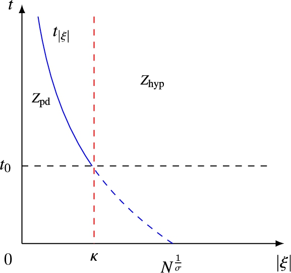
We define hyperbolic zone and pseudo differential zone respectively on the phase space as follows: $\begin{array}{l} Z_{hyp} (N) : = {(t, ξ) \in [t_{0}, \infty) \times R^{n} : (1 + t) | ξ |^{σ} ⩾ N}, \\ Z_{pd} (N) : = {(t, ξ) \in [t_{0}, \infty) \times R^{n} : (1 + t) | ξ |^{σ} ⩽ N}, \end{array}$ with the positive constants $t_{0}$ and N to be chosen later (see Fig. 1).

Fig. 1.

Sketch of the zones.

We define $\begin{array}{l} (12) & S = \{\begin{matrix} t_{| ξ |} & if | ξ | ⩽ κ, \\ t_{0} & if | ξ | ⩾ κ, \end{matrix} \end{array}$ where $t_{| ξ |}$ is the separating line between the zones is defined by $\begin{array}{l} t_{| ξ |} = \{\begin{matrix} \frac{N}{| ξ |^{σ}} - 1 & if | ξ |^{σ} ⩽ N, \\ 0 & if | ξ |^{σ} ⩾ N . \end{matrix} \end{array}$

3.1. Proof of Theorem 1

3.1.1. Considerations in $Z_{hyp} (N)$

Lemma 1.
We assume Hypothesis 1 . Then, we have the following estimate in $Z_{hyp} (N)$ : $\begin{matrix} E (t, ξ) ≲ exp (- \int_{S}^{t} μ (s) d s) E (S, ξ) for all t ⩾ S, \end{matrix}$ where $E (t, ξ)$ is defined by ( 11 ) and S is given by ( 12 ).
Proof.
Let us introduce $\begin{array}{l} (13) & δ (t) : = exp (\int_{S}^{t} b (τ) d τ) . \end{array}$ First, we multiply our equation (10) by $δ (t) {\overline{\hat{u}}}_{t}$ and extract the real part as follows: $\begin{matrix} δ (t) Re ({\hat{u}}_{t t} {\overline{\hat{u}}}_{t}) + | ξ |^{2 σ} δ (t) Re ({\hat{u}}_{t} \overline{\hat{u}}) + δ (t) b (t) | {\hat{u}}_{t} |^{2} = 0 . \end{matrix}$ Using $\begin{matrix} Re ({\hat{u}}_{t t} {\overline{\hat{u}}}_{t}) = \frac{1}{2} \frac{d}{d t} | {\hat{u}}_{t} |^{2} and Re ({\hat{u}}_{t} \overline{\hat{u}}) = \frac{1}{2} \frac{d}{d t} | \hat{u} |^{2}, \end{matrix}$ we can rewrite the last statement as follows: $\begin{matrix} δ (t) \frac{1}{2} \frac{d}{d t} (| {\hat{u}}_{t} |^{2} + | ξ |^{2 σ} | \hat{u} |^{2}) + δ (t) b (t) | {\hat{u}}_{t} |^{2} = 0 . \end{matrix}$ Then, we have $\begin{matrix} δ (t) \frac{d}{d t} E (t, ξ) + δ (t) b (t) | {\hat{u}}_{t} |^{2} = 0 . \end{matrix}$ We may rewrite the last equality in the following way: $\begin{matrix} \frac{d}{d t} (δ (t) E (t, ξ)) + δ (t) b (t) | {\hat{u}}_{t} |^{2} = δ^{'} (t) E (t, ξ), \end{matrix}$ and by using (13), we have $\begin{matrix} \frac{d}{d t} (δ (t) E (t, ξ)) + δ (t) b (t) | {\hat{u}}_{t} |^{2} = δ (t) b (t) E (t, ξ) . \end{matrix}$ If write the statement of $E (t, ξ)$ explicitly on the right hand-side of the last equality, we get $\begin{array}{l} (14) & \frac{d}{d t} (δ (t) E (t, ξ)) = \frac{1}{2} | ξ |^{2 σ} δ (t) b (t) | \hat{u} |^{2} - \frac{1}{2} δ (t) b (t) | {\hat{u}}_{t} |^{2} . \end{array}$ Now we multiply (10) by $K (t) δ (t) \overline{\hat{u}}$ , with the function $K (t)$ to be chosen later, and extract the real part in the following way: $\begin{array}{l} (15) & a (t) Re ({\hat{u}}_{t t} \hat{u}) + | ξ |^{2 σ} a (t) | \hat{u} |^{2} + a (t) b (t) Re ({\hat{u}}_{t} \overline{\hat{u}}) = 0, \end{array}$ where $a (t) : = K (t) δ (t)$ . Here we can use $\begin{array}{l} Re ({\hat{u}}_{t t} \hat{u}) = \frac{d}{d t} Re ({\hat{u}}_{t} \overline{\hat{u}}) - | {\hat{u}}_{t} |^{2}, \\ (16) & \begin{matrix} a (t) Re ({\hat{u}}_{t t} \hat{u}) & = a (t) \frac{d}{d t} Re ({\hat{u}}_{t} \overline{\hat{u}}) - a (t) | {\hat{u}}_{t} |^{2} \\ = \frac{d}{d t} (a (t) Re ({\hat{u}}_{t} \overline{\hat{u}})) - a^{'} (t) Re ({\hat{u}}_{t} \overline{\hat{u}}) - a (t) | {\hat{u}}_{t} |^{2} . \end{matrix} \end{array}$ Here we have $\begin{array}{l} a^{'} (t) & = K^{'} (t) δ (t) + K (t) δ^{'} (t) \\ = K^{'} (t) δ (t) + K (t) δ (t) b (t) \\ (17) & = K^{'} (t) δ (t) + a (t) b (t) . \end{array}$ Inserting (17) into (16), we find $\begin{array}{l} (18) & a (t) Re ({\hat{u}}_{t t} \hat{u}) = \frac{d}{d t} (a (t) Re ({\hat{u}}_{t} \overline{\hat{u}})) - K^{'} (t) δ (t) Re ({\hat{u}}_{t} \overline{\hat{u}}) - a (t) b (t) Re ({\hat{u}}_{t} \overline{\hat{u}}) - a (t) | {\hat{u}}_{t} |^{2} . \end{array}$ Let us insert (18) into (15). This implies $\begin{array}{l} \frac{d}{d t} (a (t) Re ({\hat{u}}_{t} \overline{\hat{u}})) = - | ξ |^{2 σ} a (t) | \hat{u} |^{2} + a (t) | {\hat{u}}_{t} |^{2} + K^{'} (t) δ (t) Re ({\hat{u}}_{t} \overline{\hat{u}}) . \end{array}$ Using $a (t) = K (t) δ (t)$ in the last statement, we arrive at $\begin{array}{l} (19) & \frac{d}{d t} (K (t) δ (t) Re ({\hat{u}}_{t} \overline{\hat{u}})) = - | ξ |^{2 σ} K (t) δ (t) | \hat{u} |^{2} + K (t) δ (t) | {\hat{u}}_{t} |^{2} + K^{'} (t) δ (t) Re ({\hat{u}}_{t} \overline{\hat{u}}) . \end{array}$ By adding (14) and (19), we find $\begin{array}{l} \frac{d}{d t} (δ (t) E (t, ξ) + K (t) δ (t) Re ({\hat{u}}_{t} \overline{\hat{u}})) \\ = (\frac{b (t)}{2} - K (t)) | ξ |^{2 σ} δ (t) | \hat{u} |^{2} + (K (t) - \frac{b (t)}{2}) δ (t) | {\hat{u}}_{t} |^{2} + K^{'} (t) δ (t) Re ({\hat{u}}_{t} \overline{\hat{u}}) . \end{array}$ Let us choose $K (t) = \frac{μ (t)}{2}$ , where μ satisfies condition (A4) in Hypothesis 1. Since $b (t) = μ (t) + ω (t)$ we have, $\begin{array}{l} \frac{d}{d t} (δ (t) E (t, ξ) + K (t) δ (t) Re ({\hat{u}}_{t} \overline{\hat{u}})) ⩽ | ω (t) | δ (t) E (t, ξ) + K^{'} (t) δ (t) Re ({\hat{u}}_{t} \overline{\hat{u}}) . \end{array}$ Integrating the last inequality on $[S, t]$ we have $\begin{array}{l} δ (t) E (t, ξ) + K (t) δ (t) Re ({\hat{u}}_{t} \overline{\hat{u}}) \\ ⩽ E (S, ξ) + K (S) | Re ({\hat{u}}_{t} (S, ξ) \overline{\hat{u} (S, ξ)}) | \\ + \int_{S}^{t} | ω (s) | δ (s) E (s, ξ) d s + \int_{S}^{t} K^{'} (s) δ (s) \underset{= \frac{1}{2} \frac{d}{d t} | \hat{u} |^{2}}{\underset{︸}{Re ({\hat{u}}_{t} \overline{\hat{u}})}} d s \\ = E (S, ξ) + K (S) | Re ({\hat{u}}_{t} (S, ξ) \overline{\hat{u} (S, ξ)}) | + \int_{S}^{t} | ω (s) | δ (s) E (s, ξ) d s \\ + \frac{1}{2} K^{'} (s) δ (s) {| \hat{u} (s, ξ) |}^{2} |_{S}^{t} - \frac{1}{2} \int_{S}^{t} (K^{″} (s) + K^{'} (s) b (s)) δ (s) {| \hat{u} (s, ξ) |}^{2} d s . \end{array}$ Thanks to condition (A3) for given $ε > 0$ , there exists $t_{0} > 0$ such that $(1 - ε) μ (t) ⩽ b (t) ⩽ (1 + ε) μ (t)$ for all $t ⩾ t_{0}$ . Hence, employing condition (A4), for $ε > 0$ sufficiently small we get $\begin{array}{l} K^{″} (s) + K^{'} (s) b (s) & = \frac{1}{2} (μ^{″} (s) + μ^{'} (s) b (s)) \\ ⩾ \frac{1}{2} (μ^{″} (s) + (1 + ε) μ^{'} (s) μ (s)) \\ = \frac{1}{4} \frac{d}{d s} (2 μ^{'} (s) + (1 + ε) μ {(s)}^{2}) ⩾ 0 for all s ⩾ t_{0} . \end{array}$ Therefore $\begin{matrix} δ (t) E (t, ξ) + K (t) δ (t) Re ({\hat{u}}_{t} \overline{\hat{u}}) ⩽ \frac{1}{2} K^{'} (t) δ (t) {| \hat{u} (t, ξ) |}^{2} + J (S, ξ) + \int_{S}^{t} | ω (s) | δ (s) E (s, ξ) d s, \end{matrix}$ where $\begin{matrix} J (S, ξ) : = E (S, ξ) + K (S) | Re ({\hat{u}}_{t} (S, ξ) \overline{\hat{u} (S, ξ)}) | - \frac{1}{2} K^{'} (S) {| \hat{u} (S, ξ) |}^{2} . \end{matrix}$ Now, by using (A2)–(A3), for given $ε \in (0, 1)$ , there exist $C > 0$ and $t_{0} > 0$ such that we may estimate $\begin{matrix} K (t) = \frac{μ (t)}{2} ⩽ \frac{b (t)}{2 (1 - ε)} ⩽ C N^{- 1} | ξ |^{σ} for all t ⩾ t_{0} \end{matrix}$ and $\begin{array}{l} | K (t) Re ({\hat{u}}_{t} \overline{\hat{u}}) | & ⩽ K (t) | {\hat{u}}_{t} | | \hat{u} | ⩽ \frac{ε}{2} | {\hat{u}}_{t} |^{2} + \frac{1}{2 ε} K {(t)}^{2} | \hat{u} |^{2} \\ ⩽ \frac{ε}{2} | {\hat{u}}_{t} |^{2} + \frac{ε}{2} | ξ |^{2 σ} | \hat{u} |^{2} ⩽ ε E (t, ξ), \end{array}$ for all $t ⩾ t_{0}$ and $N ⩾ C ε^{- 1}$ . By conditions (A2)–(A4), we may estimate $\begin{matrix} - K^{'} (t) = - \frac{1}{2} μ^{'} (t) ⩽ C μ {(t)}^{2} ⩽ ε | ξ |^{2 σ} \end{matrix}$ for all $t ⩾ t_{0}$ and $N ⩾ C ε^{- 1}$ . Hence, we get $\begin{matrix} - \frac{1}{2} K^{'} (S) {| \hat{u} (S, ξ) |}^{2} ⩽ ε E (S, ξ) . \end{matrix}$ Therefore, we have $\begin{matrix} J (S, ξ) ⩽ (1 + 2 ε) E (S, ξ) . \end{matrix}$ This implies $\begin{matrix} (20) & (1 - ε) δ (t) E (t, ξ) ⩽ (1 + 2 ε) E (S, ξ) + \int_{S}^{t} | ω (s) | δ (s) E (s, ξ) d s, \end{matrix}$ where S is defined in (12). Applying Gronwall’s inequality (cf. Lemma A.2) to (20), we get $\begin{matrix} δ (t) E (t, ξ) ⩽ (\frac{1 + 2 ε}{1 - ε}) E (S, ξ) exp (\frac{1}{1 - ε} \int_{S}^{t} | ω (s) | d s) ≲ E (S, ξ) exp (\frac{1}{1 - ε} \int_{S}^{t} | ω (s) | d s) . \end{matrix}$ Thus, since $ω \in L^{1} ([0, \infty))$ , we may conclude $\begin{matrix} E (t, ξ) ≲ \frac{1}{δ (t)} exp (\frac{1}{1 - ε} \int_{S}^{t} | ω (s) | d s) E (S, ξ) ≲ exp (- \int_{S}^{t} μ (s) d s) E (S, ξ), \end{matrix}$ where $δ (t)$ is defined in (13). □
3.1.2. Considerations in $Z_{pd} (N)$

We consider the micro-energy $\begin{matrix} U (t, ξ) = {(i \frac{N}{1 + t} \hat{u}, {\hat{u}}_{t})}^{T} . \end{matrix}$ Then, by (10) we obtain that $U = U (t, ξ)$ satisfies the following system of first order: $\begin{matrix} (21) & \partial_{t} U = \underset{A (t, ξ)}{\underset{︸}{(\begin{matrix} - \frac{1}{1 + t} & i \frac{N}{1 + t} \\ i \frac{(1 + t) | ξ |^{2 σ}}{N} & - b (t) \end{matrix})}} U . \end{matrix}$ Since we can estimate the pointwise energy $E (t, ξ)$ in (11) by $\begin{matrix} 2 E (t, ξ) \equiv {| {\hat{u}}_{t} (t, ξ) |}^{2} + | ξ |^{2 σ} {| \hat{u} (t, ξ) |}^{2} ⩽ C_{N} ({| {\hat{u}}_{t} (t, ξ) |}^{2} + \frac{1}{{(1 + t)}^{2}} {| \hat{u} (t, ξ) |}^{2}), \end{matrix}$ and, on the other hand, $\begin{matrix} {| U_{0} (ξ) |}^{2} \equiv {| {\hat{u}}_{0} (ξ) |}^{2} + {| {\hat{u}}_{1} (ξ) |}^{2} ⩽ (1 + | ξ |^{2 σ}) {| {\hat{u}}_{0} (ξ) |}^{2} + {| {\hat{u}}_{1} (ξ) |}^{2} = E (0, ξ) + {| {\hat{u}}_{0} (ξ) |}^{2}, \end{matrix}$ we have to prove a pointwise estimate for the fundamental solution $E_{pd} (t, ξ)$ to (21), i.e. $\begin{matrix} \partial_{t} E_{pd} (t, ξ) = A (t, ξ) E_{pd} (t, ξ), E_{pd} (0, ξ) = I_{2} for all 0 ⩽ t ⩽ t_{ξ} . \end{matrix}$ According to Lemma 8 in [15] and Lemma 3.9 in [18], we have to split our analysis in two cases, ${lim sup}_{t \to \infty} t b (t) < 1$ and ${lim sup}_{t \to \infty} t b (t) > 1$ , see Lemma 2 and Lemma 3, respectively. We present the proof of both Lemma in order to make the paper self-contained.

The exceptional case $b (t) = \frac{1}{1 + t} + ω (t)$ , with $ω \in L^{1}$ , for which ${lim}_{t \to \infty} t b (t) = 1$ , can be treated as in the case ${lim sup}_{t \to \infty} t b (t) < 1$ .

We introduce the following auxiliary functions that will be used to derive the estimates in $Z_{pd} (N)$ .

Definition 1.
Let $b \in C^{0} ([0, \infty))$ be a positive real-valued function. We define $\begin{array}{l} λ (t) ≐ exp (- \int_{0}^{t} b (τ) d τ), \\ Λ (t) ≐ 1 + \int_{0}^{t} λ (τ) d τ . \end{array}$
Remark 3.
If ${lim sup}_{t \to \infty} t b (t) < 1$ , then $\begin{matrix} \frac{Λ (t)}{(1 + t) \sqrt{λ (t)}} ⩽ C, \end{matrix}$ where C is a positive constant. Indeed, by hypothesis, for any given $ε \in (0, 1)$ , there exists $t_{0} > 0$ such that $(1 + t) b (t) < 1 - ε$ for all $t ⩾ t_{0}$ sufficiently large. Integration by parts yields $\begin{array}{l} Λ (t) - Λ (t_{0}) & = \int_{t_{0}}^{t} λ (τ) d τ = λ (τ) (1 + τ) |_{t_{0}}^{t} - \int_{t_{0}}^{t} (1 + τ) λ^{'} (τ) d τ \\ ⩽ λ (t) (1 + t) + \int_{t_{0}}^{t} (1 + τ) b (τ) λ (τ) d τ \\ ⩽ λ (t) (1 + t) + (1 - ε) \int_{t_{0}}^{t} λ (τ) d τ \\ ⩽ λ (t) (1 + t) + (1 - ε) Λ (t) . \end{array}$ Then, we arrive at $\begin{matrix} ε Λ (t) ⩽ Λ (t_{0}) + λ (t) (1 + t), \end{matrix}$ which gives the desired estimate $\begin{matrix} \frac{ε Λ (t)}{(1 + t) \sqrt{λ (t)}} ⩽ \frac{Λ (t_{0})}{(1 + t) \sqrt{λ (t)}} + \sqrt{λ (t)} ⩽ C, \end{matrix}$ thanks to $(1 + t) \sqrt{λ (t)}$ be an increasing function for all $t ⩾ t_{0}$ .
Lemma 2.
Let us assume Hypothesis 1 . If ${lim sup}_{t \to \infty} t b (t) < 1$ , then it holds the following estimates of the energy $E = E (t, ξ)$ in $Z_{pd} (N)$ for all $0 ⩽ t ⩽ t_{ξ}$ : $\begin{array}{l} E (t, ξ) & ⩽ C exp (- \int_{0}^{t} μ (s) d s) (E (0, ξ) + {| {\hat{u}}_{0} (ξ) |}^{2}) . \end{array}$ The same conclusion holds in the limit case $μ (t) = \frac{1}{1 + t}$ .
Proof.
We put $\begin{matrix} U = {(i η (t) \hat{u}, {\hat{u}}_{t})}^{T}, U_{0} (ξ) = {(i {\hat{u}}_{0} (ξ), {\hat{u}}_{1} (ξ))}^{T}, and U = \sqrt{λ (t)} V, \end{matrix}$ with $η (t) = {(1 + t)}^{- 1}$ and λ as in Definition 1, such that $\begin{matrix} (22) & \partial_{t} V = \underset{A (t, ξ)}{\underset{︸}{(\begin{matrix} \frac{η^{'}}{η} + \frac{b}{2} & i η \\ \frac{i | ξ |^{2 σ}}{η} & - \frac{b}{2} \end{matrix})}} V, V (0, ξ) = V_{0} (ξ) . \end{matrix}$ Since $ω \in L^{1} ([0, \infty))$ , it remains to prove that the fundamental solution $E (t, ξ)$ to (22), i.e. $\begin{matrix} \partial_{t} E = A (t, ξ) E, E (0, ξ) = I_{2}, \end{matrix}$ is bounded. If we put $E = {(E_{i j})}_{i, j = 1, 2}$ , then we can write for $j = 1, 2$ the following integral equations: $\begin{array}{l} (23) & E_{1 j} = \frac{η (t)}{\sqrt{λ (t)}} (δ_{1 j} + i \int_{0}^{t} \sqrt{λ (τ)} E_{2 j} (τ, ξ) d τ), \\ (24) & E_{2 j} = \sqrt{λ (t)} (δ_{2 j} + i \int_{0}^{t} \frac{1}{\sqrt{λ (s)}} \frac{{| ξ |}^{2 s}}{η (s)} E_{1 j} (s, ξ) d s), \end{array}$ with $δ_{j k} = 1$ if $j = k$ and $δ_{j k} = 0$ otherwise.

By replacing (24) into (23) we get $\begin{array}{l} (25) & E_{1 j} = & (I) + (II) + (III) = \frac{η (t)}{\sqrt{λ (t)}} δ_{1 j} + i \frac{η (t) (Λ (t) - 1)}{\sqrt{λ (t)}} δ_{2 j} \\ (26) & - \frac{η (t)}{\sqrt{λ (t)}} \int_{0}^{t} λ (τ) (\int_{0}^{τ} \frac{1}{\sqrt{λ (s)}} \frac{{| ξ |}^{2 σ}}{η (s)} E_{1 j} (s, ξ) d s) d τ . \end{array}$ Thanks to Remark 3, the terms (I) and (II) in (25) are bounded. We consider the term (III) in (26), that is, integrating by parts, $\begin{matrix} (III) = - \frac{η (t)}{\sqrt{λ (t)}} \int_{0}^{t} \frac{1}{\sqrt{λ (s)}} \frac{{| ξ |}^{2 σ}}{η (s)} E_{1 j} (s, ξ) (\int_{s}^{t} λ (τ) d τ) d s . \end{matrix}$ Since λ is a decreasing function and using that $(1 + t) {| ξ |}^{σ} ⩽ N$ in $Z_{pd} (N)$ we get $\begin{matrix} {| ξ |}^{2 σ} \int_{s}^{t} λ (τ) d τ ⩽ λ (s) {| ξ |}^{2 σ} (1 + t) ⩽ N {| ξ |}^{σ} λ (s) . \end{matrix}$ The estimate of $E_{1 j} (t, ξ)$ immediately follows from Lemma A.2 since $\begin{matrix} | E_{1 j} | ⩽ \frac{η (t) Λ (t)}{\sqrt{λ (t)}} exp (C N \int_{0}^{t} {| ξ |}^{σ} d s) ⩽ e^{C N^{2}} \frac{η (t) Λ (t)}{\sqrt{λ (t)}} . \end{matrix}$ By the boundedness of $E_{1 j}$ and using again that λ is a decreasing function, we can estimate (24) by $\begin{array}{l} | E_{2 j} | ⩽ \sqrt{λ (t)} (1 + C \int_{0}^{t} \frac{1}{\sqrt{λ (s)}} \frac{{| ξ |}^{2 σ}}{η (s)} d s) ⩽ C_{1} + C_{2} \int_{0}^{t} {| ξ |}^{σ} d s ⩽ C . \end{array}$ We proved that $E (t, ξ)$ is bounded, that is, $| V (t, ξ) | ⩽ C | V_{0} (ξ) |$ , therefore $\begin{matrix} E (t, ξ) ⩽ C^{'} λ (t) E (0, ξ) for all (t, ξ) \in Z_{pd} (N) . \end{matrix}$ □
Proposition 1.
We assume that ${lim inf}_{t \to \infty} (1 + t) b (t) > 1$ . This implies $λ (t) \in L^{1} ([0, \infty))$ such that $\begin{matrix} \int_{t}^{\infty} λ (τ) d τ ≲ (1 + t) λ (t) . \end{matrix}$ Moreover, $(1 + t) λ (t)$ is monotonously decreasing for large $t ⩾ t_{0}$ .

The proof of this proposition may be found in Proposition 3.7 of [18].
Lemma 3.
We assume $b ⩾ 0$ and ${lim inf}_{t \to \infty} (1 + t) b (t) > 1$ . Then, we have the following energy estimate in $Z_{pd} (N)$ : $\begin{matrix} E (t, ξ) ⩽ C {(1 + t)}^{- 2} (E (0, ξ) + {| {\hat{u}}_{0} (ξ) |}^{2}) . \end{matrix}$
Proof.
We are interested in the fundamental solution $\begin{matrix} E_{pd} (t, ξ) = (\begin{matrix} E_{pd}^{(11)} & E_{pd}^{(12)} \\ E_{pd}^{(21)} & E_{pd}^{(22)} \end{matrix}) \end{matrix}$ to the system (21). Thus, the solution $U = U (t, ξ)$ is represented as $\begin{matrix} U (t, ξ) = E_{pd} (t, ξ) U (0, ξ) for all 0 ⩽ t ⩽ t_{ξ} . \end{matrix}$ Then, by direct calculations we get for $j = 1, 2$ $\begin{array}{l} E_{pd}^{(1 j)} (t, ξ) = \frac{δ_{1 j}}{1 + t} + i \frac{N}{1 + t} \int_{0}^{t} E_{pd}^{(2 j)} (τ, ξ) d τ, \\ E_{pd}^{(2 j)} (t, ξ) = λ (t) δ_{2 j} + \frac{i λ (t) | ξ |^{2 σ}}{N} \int_{0}^{t} (1 + τ) \frac{1}{λ (τ)} E_{pd}^{(1 j)} (τ, ξ) d τ . \end{array}$ Plugging the representation for $E_{pd}^{(21)} (t, ξ)$ into the integral equation for $E_{pd}^{(11)} (t, ξ)$ gives $\begin{array}{l} E_{pd}^{(11)} (t, ξ) & = \frac{1}{1 + t} + i \frac{N}{1 + t} \int_{0}^{t} (\frac{i λ (τ) | ξ |^{2 σ}}{N} \int_{0}^{τ} (1 + θ) \frac{1}{λ (θ)} E_{pd}^{(11)} (θ, ξ) d θ) d τ \\ = \frac{1}{1 + t} - \frac{| ξ |^{2 σ}}{1 + t} \int_{0}^{t} \int_{0}^{τ} \frac{λ (τ)}{λ (θ)} (1 + θ) E_{pd}^{(11)} (θ, ξ) d θ d τ . \end{array}$ It follows $\begin{matrix} (1 + t) E_{pd}^{(11)} (t, ξ) = 1 - | ξ |^{2 σ} \int_{0}^{t} \int_{θ}^{t} \frac{λ (τ)}{λ (θ)} (1 + θ) E_{pd}^{(11)} (θ, ξ) d τ d θ . \end{matrix}$ By setting $y (t, ξ) : = (1 + t) E_{pd}^{(11)} (t, ξ)$ and applying Gronwall’s inequality we get $\begin{array}{l} | y (t, ξ) | ≲ 1 + | ξ |^{2 σ} \int_{0}^{t} \int_{θ}^{t} \underset{⩽ 1}{\underset{︸}{\frac{λ (τ)}{λ (θ)}}} | y (θ, ξ) | d τ d θ, \\ | y (t, ξ) | ≲ exp (| ξ |^{2 σ} \int_{0}^{t} \int_{0}^{t} d τ d θ) ≲ exp (| ξ |^{2 σ} {(1 + t)}^{2}) ≲ 1, \end{array}$ where we used the definition of $Z_{pd} (N)$ . Hence, we may conclude that $| E_{pd}^{(11)} (t, ξ) | ≲ {(1 + t)}^{- 1}$ . Now we consider $E_{pd}^{(21)} (t, ξ)$ . By using the estimate for $| E_{pd}^{(11)} (t, ξ) |$ we obtain $\begin{array}{l} | E_{pd}^{(21)} (t, ξ) | & ≲ | ξ |^{2 σ} \int_{0}^{t} (1 + τ) \underset{⩽ 1}{\underset{︸}{\frac{λ (t)}{λ (τ)}}} | E_{pd}^{(11)} (τ, ξ) | d τ \\ ≲ | ξ |^{2 σ} \int_{0}^{t} d τ ≲ | ξ |^{2 σ} (1 + t) ≲ {(1 + t)}^{- 1} . \end{array}$ Plugging the representation for $E_{pd}^{(22)} (t, ξ)$ into the integral equation for $E_{pd}^{(12)} (t, ξ)$ gives $\begin{array}{l} E_{pd}^{(12)} (t, ξ) & = i \frac{N}{1 + t} \int_{0}^{t} (λ (τ) + \frac{i λ (τ) | ξ |^{2 σ}}{N} \int_{0}^{τ} (1 + θ) \frac{1}{λ (θ)} E_{pd}^{(12)} (θ, ξ) d θ) d τ \\ = i \frac{N}{1 + t} \int_{0}^{t} λ (τ) d τ - \frac{| ξ |^{2 σ}}{1 + t} \int_{0}^{t} \int_{0}^{τ} \frac{λ (τ)}{λ (θ)} (1 + θ) E_{pd}^{(12)} (θ, ξ) d θ d τ . \end{array}$ Then, we have $\begin{array}{l} (1 + t) | E_{pd}^{(12)} (t, ξ) | & ≲ \int_{0}^{t} λ (τ) d τ + | ξ |^{2 σ} \int_{0}^{t} \int_{θ}^{t} \underset{⩽ 1}{\underset{︸}{\frac{λ (τ)}{λ (θ)}}} (1 + θ) | E_{pd}^{(12)} (θ, ξ) | d τ d θ \\ ≲ λ (0) + | ξ |^{2 σ} \int_{0}^{t} \int_{0}^{t} (1 + θ) | E_{pd}^{(12)} (θ, ξ) | d τ d θ, \end{array}$ where we used Proposition 1. Then, applying Gronwall’s inequality from Lemma A.2 we get the estimate $\begin{array}{l} (1 + t) | E_{pd}^{(12)} (t, ξ) | ≲ exp (| ξ |^{2 σ} \int_{0}^{t} \int_{0}^{t} d τ d θ) ≲ exp (| ξ |^{2 σ} {(1 + t)}^{2}) ≲ 1, \end{array}$ where we used the definition of $Z_{pd} (N)$ . Thus, we get $| E_{pd}^{(12)} (t, ξ) | ≲ {(1 + t)}^{- 1}$ . Finally, let us consider $E_{pd}^{(22)} (t, ξ)$ by using the estimate for $| E_{pd}^{(12)} (t, ξ) |$ . It holds $\begin{array}{l} | E_{pd}^{(22)} (t, ξ) | & ≲ λ (t) + \frac{| ξ |^{2 σ}}{N} \int_{0}^{t} \underset{⩽ 1}{\underset{︸}{\frac{λ (t)}{λ (τ)}}} (1 + τ) | E_{pd}^{(12)} (τ, ξ) | d τ \\ ≲ λ (t) + \frac{| ξ |^{2 σ}}{N} \int_{0}^{t} d τ ≲ λ (t) + | ξ |^{2 σ} (1 + t) . \end{array}$ Then, we have $\begin{array}{l} (1 + t) | E_{pd}^{(22)} (t, ξ) | & ≲ (1 + t) λ (t) + | ξ |^{2 σ} {(1 + t)}^{2} ≲ 1 . \end{array}$ This shows that $| E_{pd}^{(22)} (t, ξ) | ≲ {(1 + t)}^{- 1}$ . This completes the proof. □

By using the Parseval–Plancherel theorem and the pointwise estimates of the partial Fourier transform of solutions in the Fourier space, the proof of Theorem 1 follows immediately from the following Corollary. Corollary 1.
Under the assumption of Hypothesis 1 we have the following estimates of the energy $E = E (t, ξ)$ in $Z_{hyp} (N)$ for all $t ⩾ S$ : $\begin{array}{l} E (t, ξ) & ≲ exp (- \int_{S}^{t} μ (s) d s) E (S, ξ), \end{array}$ where S is given by ( 12 ) with sufficiently large $t_{0}$ . In $Z_{pd} (N)$ , we have for all $t \in [0, t_{ξ}]$ $\begin{array}{l} E (t, ξ) ≲ \{\begin{matrix} exp (- \int_{0}^{t} μ (s) d s) (E (0, ξ) + | {\hat{u}}_{0} (ξ) |^{2}) & if {lim sup}_{t \to \infty} (1 + t) b (t) < 1, \\ {(1 + t)}^{- 2} (E (0, ξ) + | {\hat{u}}_{0} (ξ) |^{2}) & if {lim inf}_{t \to \infty} (1 + t) b (t) > 1 . \end{matrix} \end{array}$ Then, for all $t ⩾ t_{0}$ we arrive at $\begin{matrix} E (t, ξ) ⩽ C exp (- \int_{0}^{t} μ (s) d s) (E (0, ξ) + {| \hat{u_{0}} (ξ) |}^{2}) . \end{matrix}$
Proof.
First, we recall that the pointwise energy is bounded for $t \in [0, t_{0}]$ , i.e. $E (t, ξ) ⩽ C E (0, ξ)$ for all $t \in [0, t_{0}]$ . By Hypotheses of $ω \in L^{1} ([0, \infty))$ and ${lim sup}_{t \to \infty} (1 + t) b (t) < 2$ , there exists $t_{0} > 0$ sufficiently large such that $\begin{matrix} exp (- \int_{t_{0}}^{t} μ (s) d s) ⩾ C exp (- \int_{t_{0}}^{t} b (s) d s) ⩾ C {(1 + t)}^{- 2} for all t ⩾ t_{0} . \end{matrix}$ For $| ξ | ⩾ κ$ the conclusion follows from the estimate in $Z_{hyp} (N)$ zone. For $| ξ | ⩽ κ$ and for $t ⩽ t_{ξ}$ we use the estimate in $Z_{pd} (N)$ zone, whereas for $t ⩾ t_{ξ}$ we have to glue the estimates in both zones, namely, $\begin{array}{l} E (t, ξ) & ⩽ C exp (- \int_{t_{ξ}}^{t} μ (s) d s) E (t_{ξ}, ξ) \\ ⩽ C exp (- \int_{t_{ξ}}^{t} μ (s) d s) (- \int_{0}^{t_{ξ}} μ (s) d s) (E (0, ξ) + {| \hat{u_{0}} (ξ) |}^{2}) \\ ⩽ C exp (- \int_{0}^{t} μ (s) d s) (E (0, ξ) + {| \hat{u_{0}} (ξ) |}^{2}) . \end{array}$ □

3.2. Proof of Theorem 2

In this section we may take $t_{0} = 0$ in $Z_{hyp} (N)$ (see Fig. 1).

3.2.1. Considerations in $Z_{hyp} (N)$

Lemma 4.
Under the assumption of Hypothesis 2 , we have the following estimate in $Z_{hyp} (N)$ : $\begin{matrix} E (t, ξ) ⩽ C \frac{{(1 + t_{ξ})}^{2}}{{(1 + t)}^{2}} (| ξ |^{2 σ} {| \hat{u} (t_{ξ}, ξ) |}^{2} + {| {\hat{u}}_{t} (t_{ξ}, ξ) |}^{2}) for all t ⩾ t_{ξ}, \end{matrix}$ where $E (t, ξ)$ is defined in ( 11 ).
Proof.
If we multiply both sides of (10) by ${\hat{u}}_{t}$ , we get $\begin{matrix} (27) & \frac{1}{2} \frac{d}{d t} (| {\hat{u}}_{t} |^{2} + | ξ |^{2 σ} | \hat{u} |^{2}) + b (t) | {\hat{u}}_{t} |^{2} = 0 . \end{matrix}$ If we integrate the equation (27) on $[S, T]$ , we arrive at $\begin{matrix} E (T, ξ) + \int_{S}^{T} b (s) | u_{t} |^{2} d s = E (S, ξ) . \end{matrix}$ Let $Z \subset [0, \infty) \times R^{n}$ and define $K : Z \to [0, \infty)$ . Now we multiply both sides of (27) by $K (t, ξ) \hat{u}$ . Then, we have for $(t, ξ) \in Z$ $\begin{array}{l} \frac{d}{d t} (K (t, ξ) Re ({\hat{u}}_{t} \hat{u})) + b (t) K (t, ξ) Re ({\hat{u}}_{t} \hat{u}) + K (t, ξ) | ξ |^{2 σ} | \hat{u} |^{2} \\ (28) & = K (t, ξ) | {\hat{u}}_{t} |^{2} + (\frac{d}{d t} K (t, ξ)) Re ({\hat{u}}_{t} \hat{u}) . \end{array}$ Let us integrate (28) on $[S, T]$ . Then, we may write $\begin{array}{l} \int_{S}^{T} K (s, ξ) | ξ |^{2 σ} | \hat{u} |^{2} d s & : = \sum_{k = 1}^{4} I_{k} (S, T, ξ), \end{array}$ where $\begin{array}{l} I_{1} (S, T, ξ) : = \int_{S}^{T} K (s, ξ) | {\hat{u}}_{t} |^{2} d s, \\ I_{2} (S, T, ξ) : = \int_{S}^{T} (\frac{d}{d s} K (s, ξ)) Re ({\hat{u}}_{t} \hat{u}) d s, \\ I_{3} (S, T, ξ) : = - \int_{S}^{T} \frac{d}{d s} (K (s, ξ) Re ({\hat{u}}_{t} \hat{u})) d s, \\ I_{4} (S, T, ξ) : = - \int_{S}^{T} b (s) K (s, ξ) Re ({\hat{u}}_{t} \hat{u}) d s . \end{array}$ We define the multiplier of the energy in $Z_{hyp} (N)$ as follows: $\begin{matrix} K (t, ξ) : = μ (t) . \end{matrix}$ We get for $I_{1} (S, T, ξ)$ the estimate $\begin{array}{l} I_{1} (S, T, ξ) & = \int_{S}^{T} K (s, ξ) | {\hat{u}}_{t} |^{2} d s = \int_{S}^{T} μ (s) | {\hat{u}}_{t} |^{2} d s \\ ⩽ (1 + ε) \int_{S}^{T} b (s) | {\hat{u}}_{t} |^{2} d s ⩽ (1 + ε) E (S, ξ), \end{array}$ where due to condition (B2) we have used $μ (t) ⩽ (1 + ε) b (t)$ . The estimate for $I_{2} (S, T, ξ)$ satisfies $\begin{array}{l} I_{2} (S, T, ξ) & = \int_{S}^{T} (\frac{d}{d s} K (s, ξ)) Re ({\hat{u}}_{t} \hat{u}) d s ⩽ C \int_{S}^{T} | {\hat{u}}_{t} | \frac{μ (s)}{1 + s} | \hat{u} | d s \\ ⩽ C ϵ \int_{S}^{T} μ (s) | {\hat{u}}_{t} |^{2} d s + \frac{C}{ϵ} \int_{S}^{T} μ (s) \frac{1}{{(1 + s)}^{2}} | \hat{u} |^{2} d s \\ ⩽ C ϵ (1 + ε) E (S, ξ) + \frac{C}{N^{2} ϵ} \int_{S}^{T} μ (s) | ξ |^{2 σ} | \hat{u} |^{2} d s \\ ⩽ C ϵ (1 + ε) E (S, ξ) + ϵ \int_{S}^{T} μ (s) | ξ |^{2 σ} | \hat{u} |^{2} d s, \end{array}$ for any $ϵ > 0$ and $N^{2} ⩾ \frac{C}{ϵ^{2}}$ . Now, using the estimate $\begin{array}{l} | K (t, ξ) Re ({\hat{u}}_{t} \hat{u}) | & ⩽ \frac{β}{1 + t} | {\hat{u}}_{t} | | \hat{u} | ⩽ β ϵ | u_{t} |^{2} + \frac{β}{ϵ {(1 + t)}^{2}} | \hat{u} |^{2} \\ ⩽ β ϵ | u_{t} |^{2} + \frac{β}{N^{2} ϵ} | ξ |^{2 σ} | \hat{u} |^{2} ⩽ 2 β ϵ E (t, ξ), \end{array}$ for $N^{2} ⩾ \frac{1}{ϵ^{2}}$ , then we arrive at the following estimate for $I_{3} (S, T, ξ)$ : $\begin{array}{l} I_{3} (S, T, ξ) & = - \int_{S}^{T} \frac{d}{d s} (K (s, ξ) Re ({\hat{u}}_{t} \hat{u})) d s \\ = K (S, ξ) Re ({\hat{u}}_{t} \hat{u}) - K (T, ξ) Re ({\hat{u}}_{t} \hat{u}) \\ ⩽ K (S, ξ) | {\hat{u}}_{t} | | \hat{u} | + K (T, ξ) | {\hat{u}}_{t} | | \hat{u} | \\ ⩽ 2 β ϵ E (S, ξ) + 2 β ϵ E (T, ξ) ⩽ 4 β ϵ E (S, ξ) for T ⩾ S, \end{array}$ where we have the last estimate, because the energy is decreasing. Finally, we estimate $I_{4} (S, T, ξ)$ as follows: $\begin{array}{l} I_{4} (S, T, ξ) & = \int_{S}^{T} b (s) K (s, ξ) Re ({\hat{u}}_{t} \hat{u}) d s ⩽ ϵ \int_{S}^{T} b (s) | {\hat{u}}_{t} |^{2} d s + \frac{1}{ϵ} \int_{S}^{T} b (s) K {(s, ξ)}^{2} | \hat{u} |^{2} d s \\ ⩽ ϵ E (S, ξ) + \frac{2 β^{2}}{ϵ} \int_{S}^{T} μ (s) \frac{1}{{(1 + s)}^{2}} | \hat{u} |^{2} d s \\ ⩽ ϵ E (S, ξ) + \frac{2 β^{2}}{ϵ} \frac{1}{N^{2}} \int_{S}^{T} μ (s) | ξ |^{2 σ} | \hat{u} |^{2} d s \\ ⩽ ϵ E (S, ξ) + ϵ \int_{S}^{T} μ (s) | ξ |^{2 σ} | \hat{u} |^{2} d s, \end{array}$ with $N ⩾ \frac{\sqrt{2} β}{ϵ}$ . Therefore, using the derived estimates from $I_{1} (S, T, ξ)$ to $I_{4} (S, T, ξ)$ , we get $\begin{array}{l} (1 - 2 ϵ) \int_{S}^{T} K (s, ξ) | ξ |^{2 σ} | \hat{u} |^{2} d s & ⩽ (1 + ε + C ϵ (1 + ε) + 4 β ϵ + ϵ) E (S, ξ) \\ ⩽ (1 + 2 ε) E (S, ξ), \end{array}$ where $C ϵ (1 + ε) + 4 β ϵ + ϵ ⩽ ε$ with $ϵ > 0$ is sufficiently small. Consequently, we conclude $\begin{array}{l} \int_{S}^{T} μ (s) E (s, ξ) d s = \int_{S}^{T} μ (s) \underset{: = E (s, ξ)}{\underset{︸}{\frac{1}{2} (| u_{t} |^{2} + | ξ |^{2 σ} | \hat{u} |^{2})}} d s ⩽ (\frac{1}{2} + ε + \frac{1}{2} + \frac{ε}{2}) E (S, ξ) . \end{array}$ Then, applying Lemma A.1 we can get the following estimate: $\begin{matrix} E (t, ξ) ⩽ C exp (- \frac{ϵ_{0}}{C^{'}} \int_{t_{ξ}}^{t} μ (s) d s) E (t_{ξ}, ξ) ⩽ C \frac{{(1 + t_{ξ})}^{2}}{{(1 + t)}^{2}} E (t_{ξ}, ξ), \end{matrix}$ for all $t ⩾ t_{ξ}$ , for any $ϵ_{0} \in (0, 1)$ and $C^{'} : = 1 + 3 ε / 2$ . Here from conditions (B1)–(B2) we used that $μ (t) = \frac{β}{1 + t}$ with $β > 2 + 3 ε$ . □

We may conclude the proof of Theorem 2 easily by Lemma 3 and Lemma 4 after using the Parseval–Plancherel theorem.

1. Case: $| ξ | ⩾ N^{\frac{1}{σ}}$

Then, the statement of Lemma 4 implies immediately $\begin{matrix} E (t, ξ) ⩽ C {(1 + t)}^{- 2} (| ξ |^{2 σ} {| \hat{u} (0, ξ) |}^{2} + {| {\hat{u}}_{t} (0, ξ) |}^{2}) for all t ⩾ 0 . \end{matrix}$

2. Case: $| ξ | ⩽ N^{\frac{1}{σ}}$

We may use Lemma 3 for $0 ⩽ t ⩽ t_{ξ}$ , whereas the statements of Lemma 4 and Lemma 3 give immediately $\begin{array}{l} E (t, ξ) & ⩽ C \frac{{(1 + t_{ξ})}^{2}}{{(1 + t)}^{2}} (| ξ |^{2 σ} {| \hat{u} (t_{ξ}, ξ) |}^{2} + {| {\hat{u}}_{t} (t_{ξ}, ξ) |}^{2}) \\ ⩽ C \frac{{(1 + t_{ξ})}^{2}}{{(1 + t)}^{2}} {(1 + t_{ξ})}^{- 2} (E (0, ξ) + {| {\hat{u}}_{0} (ξ) |}^{2}) \\ ⩽ C {(1 + t)}^{- 2} (E (0, ξ) + {| {\hat{u}}_{0} (ξ) |}^{2}) for all t ⩾ t_{ξ} . \end{array}$ This completes the proof of Theorem 2.
4. Concluding remarks

4.1. The limit case

For the sake of simplicity, let us consider the Cauchy problem (8) with $σ = 1$ $\begin{matrix} (29) & \{\begin{matrix} u_{t t} - Δ u + b (t) u_{t} = 0, (t, x) \in [0, \infty) \times R^{n}, \\ u (0, x) = u_{0} (x), u_{t} (0, x) = u_{1} (x), x \in R^{n}, \end{matrix} \end{matrix}$ where $\begin{matrix} b (t) = \frac{2}{1 + t} + ω (t) and ω \in L^{1} ([0, \infty)) . \end{matrix}$ If we use the transformation $\begin{matrix} u (t, x) = {(1 + t)}^{- 1} v (t, x), \end{matrix}$ then $v = v (t, x)$ solves the following Cauchy problem $\begin{matrix} (30) & \{\begin{matrix} v_{t t} - Δ v + ω (t) v_{t} - \frac{ω (t)}{1 + t} v = 0, (t, x) \in [0, \infty) \times R^{n}, \\ v (0, x) = u_{0} (x), v_{t} (0, x) = u_{0} (x) + u_{1} (x), x \in R^{n} . \end{matrix} \end{matrix}$ Since $ω \in L^{1} ([0, \infty))$ , then the energy for solutions to (30) is bounded, see Theorem 2 in [4]. Therefore, if $u_{0} \in H^{σ}$ and $u_{1} \in L^{2}$ , the energy solution to (29) satisfies $\begin{matrix} E (t) ⩽ C {(1 + t)}^{- 2} (E (0) + ‖ u_{0} ‖_{L^{2}}^{2}) for all t ⩾ 0 . \end{matrix}$

Footnotes

Acknowledgements

The authors thank Edson Cilos Vargas Júnior (UFSC), Cleverson Roberto da Luz (UFSC) and Michael Reissig (TU Freiberg) for theirs numerous hints and discussions in the preparation of the paper. The authors also would like to thank the referees for their careful reading of the paper and valuable comments.

Halit S. Aslan has been supported by Grant 2021/01743-3 from “Fundação de Amparo à Pesquisa do Estado de São Paulo (FAPESP)”. Marcelo R. Ebert is partially supported by Grant 2020/08276-9 from “FAPESP” and Grant 304408/2020-4 from “Conselho Nacional de Desenvolvimento Científico e Tecnológico (CNPq)”.

Appendix

The following lemma plays a fundamental role in order to prove our main theorems. The proof may be found in Lemma 2.1 of [12].

For the proof see Theorem 1.3.1 in [9].

References

Boiti and

Manfrin, On the asymptotic boundedness of the energy of solutions of the wave equation

u_{t t} - a (t) Δ u = 0

, Ann. Univ. Ferrara 58 (2012), 251–289. doi:10.1007/s11565-012-0148-6.

R.C.

Charão,

C.R.

da Luz and

Ikehata, Sharp decay rates for wave equations with a fractional damping via new method in the Fourier space, J. Math. Anal. Appl. 408 (2013), 247–255. doi:10.1016/j.jmaa.2013.06.016.

Colombini, Energy estimates at infinity for hyperbolic equations with oscillating coefficients, J. Differential Equations 231(2) (2006), 598–610. doi:10.1016/j.jde.2006.05.014.

D’Abbicco and

M.R.

Ebert, A class of dissipative wave equations with time-dependent speed and damping, J. Math. Anal. Appl. 399 (2013), 255–278.

D’Abbicco and

M.R.

Ebert, A classification of structural dissipations for evolution operators, Math. Methods Appl. Sci. 39 (2016), 2558–2582. doi:10.1002/mma.3713.

M.R.

Ebert and

Reissig, The influence of oscillations on global existence for a class of semi-linear wave equations, Math. Methods Appl. Sci. 34 (2011), 1289–1307. doi:10.1002/mma.1430.

Hirosawa, On the asymptotic behavior of the energy for the wave equation with time depending coefficients, Math. Ann. 339(4) (2007), 819–838. doi:10.1007/s00208-007-0132-0.

Hirosawa and

Wirth,

C^{m}

-theory of damped wave equations with stabilisation, J. Math. Anal. Appl. 343(2) (2008), 1022–1035. doi:10.1016/j.jmaa.2008.02.024.

B.G.

Pachpatte, Inequalities for Differential and Integral Equations, Mathematics in Science and Engineering, Vol. 197, Academic Press, Inc., San Diego, CA, 1998.

10.

Reissig and

Smith,

L^{p} - L^{q}

estimate for wave equation with bounded time-dependent coefficient, Hokkaido Math. J. 34(3) (2005), 541–586. doi:10.14492/hokmj/1285766286.

11.

Reissig and

Yagdjian, About the influence of oscillations on Strichartz-type decay estimates, in: Partial Differential Operators (Torino, 2000), Rem. Sem. Mat. Univ. Politec. Torino, Vol. 58, 2000, pp. 375–388.

12.

E.C.

Vargas Júnior and

C.R.

da Luz, σ-evolution models with low regular time-dependent non-effective structural damping, Asymptotic Analysis 119 (2020), 61–86. doi:10.3233/ASY-191566.

13.

E.C.

Vargas Júnior and

C.R.

da Luz, σ-evolution models with low regular time-dependent effective structural damping, J. Math. Anal. Appl. 499(2) (2021), 125030. doi:10.1016/j.jmaa.2021.125030.

14.

Wirth, Solution representations for a wave equation with weak dissipation, Math. Methods Appl. Sci. 27(1) (2004), 101–124. doi:10.1002/mma.446.

15.

Wirth, Wave equations with time-dependent dissipation I. Non-effective dissipation, J. Differential Equations 222(2) (2006), 487–514. doi:10.1016/j.jde.2005.07.019.

16.

Wirth, Wave equations with time-dependent dissipation II. Effective dissipation, J. Differential Equations 232(1) (2007), 74–103. doi:10.1016/j.jde.2006.06.004.

17.

Wirth, On the influence of time-periodic dissipation on energy and dispersive estimates, Hiroshima Math. J. 38(3) (2008), 397–410. doi:10.32917/hmj/1233152777.

18.

Wirth, Asymptotic properties of solutions to wave equations with time-dependent dissipation, PhD thesis, TU Bergakademie Freiberg, 2004, 146 pp.

On the asymptotic behavior of the energy for evolution models with oscillating time-dependent damping

Abstract

Keywords

1. Introduction

1.1. Main purpose of the paper

2.1. Models with the behavior of energy solutions determined at high frequencies

3.1.1. Considerations in Z hyp ( N )

3.2.1. Considerations in Z hyp ( N )

4.1. The limit case

Footnotes

Acknowledgements

Appendix

References

3.1.1. Considerations in $Z_{hyp} (N)$

3.2.1. Considerations in $Z_{hyp} (N)$