Puiseux asymptotic expansions for convection-dominated transport problems in thin graph-like networks: Strong boundary interactions

Abstract

This article completes the study of the influence of the intensity parameter α in the boundary condition $ε \partial_{ν_{ε}} u_{ε} - u_{ε} \vec{V_{ε}} \cdot ν_{ε} = ε^{α} φ_{ε}$ given on the boundary of a thin three-dimensional graph-like network consisting of thin cylinders that are interconnected by small domains (nodes) with diameters of order $O (ε)$ . Inside of the thin network a time-dependent convection-diffusion equation with high Péclet number of order $O (ε^{- 1})$ is considered. The novelty of this article is the case of $α < 1$ , which indicates a strong intensity of physical processes on the boundary, described by the inhomogeneity $φ_{ε}$ (the cases $α = 1$ and $α > 1$ were previously studied by the same authors).

A complete Puiseux asymptotic expansion is constructed for the solution $u_{ε}$ as $ε \to 0$ , i.e., when the diffusion coefficients are eliminated and the thin network shrinks into a graph. Furthermore, the corresponding uniform pointwise and energy estimates are proved, which provide an approximation of the solution with a given accuracy in terms of the parameter ε.

Keywords

Asymptotic expansion convection-diffusion problem boundary interactions thin graph-like junction hyperbolic limit model

1. Introduction

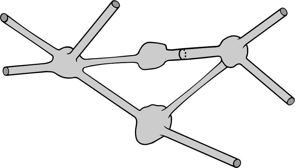
In this paper we continue our study [20,21] of parabolic transport problems for some species’ concentration in graph-like networks. For ε being a small parameter, these consist of thin cylinders that are interconnected by small domains (nodes) of order $O (ε)$ in diameter, see Fig. 1. The parameter ε is not only characterising the geometry of the thin network but also the strength of certain physical processes. First, we consider a high Péclet number regime of order $O (ε^{- 1})$ , i.e. a high ratio of convective to diffusive transport rates. This assumption leads to a re-scaled diffusion operator in the parabolic differential equation $\begin{matrix} (1.1) & \partial_{t} u_{ε} - ε Δ_{x} u_{ε} + {div}_{x} (\vec{V_{ε}} u_{ε}) = 0, \end{matrix}$ governing the unknown species concentration $u_{ε}$ . In (1.1), $\vec{V_{ε}}$ is a given convective vector field with small transversal velocity components. In order to study additionally the influence of external influences via boundary interactions, in the paper [21] an additional parameter α was introduced in the inhomgeneous boundary conditions $\begin{matrix} ε \partial_{ν_{ε}} u_{ε} - u_{ε} \vec{V_{ε}} \cdot ν_{ε} = ε^{α} φ_{ε}^{(i)}, i \in {0, 1, \dots, M}, \end{matrix}$ which hold both on the lateral surfaces of thin cylinders and on the boundaries of nodes forming the thin network. Here, a given function $φ^{(i)}$ describes physical processes on the surface of the ith component of the network.

Fig. 1.

Network of thin cylinders connected by nodes of arbitrary geometry.

Three qualitatively different cases can be identified for the asymptotic behaviour (as $ε \to 0$ ) of the solution $u_{ε}$ depending on the value of α, namely $α > 1$

low intensity of boundary processes (if $α ⩾ 2$ they can simply be ignored, if $α \in (1, 2)$ their influence appears in the second-order terms of the asymptotics);

α = 1

moderate intensity, then the boundary processes directly affect the first terms ${w_{0}^{(i)}}_{i}$ of the asymptotics, which represent the solution of the limit problem consisting of first-order hyperbolic equations $\begin{matrix} (1.2) & \partial_{t} w_{0}^{(i)} (x_{i}, t) + \partial_{x_{i}} (v_{i}^{(i)} (x_{i}, t) w_{0}^{(i)} (x_{i}, t)) = - {\hat{φ}}^{(i)}, \end{matrix}$ each of which is defined on the i-th edge of the corresponding metric graph, to which the thin network shrinks (here $- {\hat{φ}}^{(i)}$ is the limit transformation of the boundary interaction $φ^{(i)}$ into the right-hand side of the differential equation);

α < 1

strong intensity (it was only noted in the conclusion of [21] that the question of finding the asymptotics remains open and one should expect that the solution will be unbounded as $ε \to 0$ ).

In this paper we present a complete analysis of the latter, qualitatively different case whereas the first two ones have been analyzed in [21].

Studying the influence of inhomogeneous Neumann or Fourier boundary conditions on the processes in the entire domain is a very timely task, especially in regions with complex structures, e.g., see papers [1,4–9,12–14,23] for perforated domains, [2,15,17] for thin domains, [3,19] for domains with rapidly oscillating boundaries, [10,11,22] for thick junctions or domains with a highly oscillating boundary. The problems considered in these works are mathematical models of various reaction-diffusion, adsorption and transport phenomena in hydrogeology, chemistry, biology, medicine, and thermal conductivity.

In the vast majority of these works, the intensity of the processes at the boundaries is not high, which leads to the appearance of an additional term in the corresponding limit differential equation (it depends on the ratio between the total size of the surfaces and the intensity of the processes on these surfaces). In [10] the author gave an example of a boundary-value problem with a large boundary interaction in a domain with a highly oscillating boundary and proved that the solution becomes unbounded as the oscillation parameter tends to zero. Additional assumptions that guarantee a priori estimates for the solution regardless of the small parameter can help to prove the convergence theorem even for large boundary interactions (see, e.g., [11]). However, in the general case, physical processes at the boundary of regions with a complex structure can provoke cardinal changes in the global phenomenon throughout the region.

The principal novelty of the present paper is the study of the impact of strong boundary interactions (the case $α < 1$ and without any additional assumptions guaranteeing a priori estimates) on the asymptotic behaviour (as $ε \to 0$ ) of the solution to the parabolic convection-dominated transport problem in a thin graph-like network.

To do this, we use the asymptotic expansion method, which is a very powerful tool for studying various perturbed problems. Usually the corresponding first term in the expansion gives the basic limiting behavior for the solution of interest; the subsequent terms allow to estimate the sensitivity of the model to smaller scale perturbations. Therefore, convergence results used in studies of perturbed models may not be acceptable in cases where the values of the perturbation parameters are not small enough. Asymptotic expansions allow the influence of other features of the model to be taken into account through higher-order terms in the expansions, and improve the accuracy of the corresponding numerical procedures by combining them with asymptotic results. It should be noted that in asymptotic analysis it is very important to guess the form of the asymptotic ansatz, which is affected by various parameters of the problem (see. e.g., [18,23]).

In the present work we compose effective recurrent algorithms for constructing asymptotic Puiseux expansions. Such series are a generalization of power series that allow negative and fractional exponents of the indeterminate; in our case, these are real exponents of the parameter ε, which depend on the parameter α. We show that the principal part of the Puiseux series (it consists of unbounded coefficients as $ε \to 0$ ; see Definition 3.1), which determines the main behaviour of the solution in the ith thin cylinder of the network, is as follows $\begin{matrix} (1.3) & ε^{α - 1} w_{α - 1}^{(i)} (x_{i}, t) + ε^{α} w_{α}^{(i)} (x_{i}, t) + \sum_{k = 2}^{- ⌊ α ⌋} ε^{α + k - 1} (w_{α + k - 1}^{(i)} (x_{i}) + u_{α + k - 1}^{(i)} (x_{i}, \frac{{\overline{x}}_{i}}{ε}, t)) . \end{matrix}$ Note that, for $α \in [0, 1)$ , there is only one term $ε^{α - 1} w_{α - 1}^{(i)}$ in the principal part. The coefficients ${w_{α - 1}^{(i)}}_{i}$ form the solution to the corresponding hyperbolic transport problem on the graph, the right-hand sides of which are the averaged characteristics of the boundary interactions (see (3.27)). The coefficients ${w_{α}^{(i)}}_{i}$ represent the solution to the hyperbolic transport problem (3.35), and they take into account interactions on the node boundary, physical processes inside the node and geometric characteristics of the network through the special gluing condition $\begin{matrix} (1.4) & \sum_{i} v_{i} h_{i}^{2} w_{α}^{(i)} (0, t) = d_{α} (t) \end{matrix}$ at the graph vertex, where $d_{α} (t)$ is determined in (3.34).

It is worth noting another interesting feature in the study of boundary-value problems with a predominance of convection in thin networks, namely that the corresponding first-order hyperbolic problems for the coefficients of the asymptotic expansion have only a Kirchhoff-type transmission condition (similar to (1.4)) at the graph vertices; no other condition, commonly called the continuity condition. This means that such solutions, generally speaking, are not continuous at the vertices, which is explained by the wave-particle duality of first-order hyperbolic differential equations (for more details see the conclusion section of our paper [20]). To neutralize this duality and to ensure continuity of the approximation in the vicinities of nodes, a special node-layer part of the asymptotics is introduced whose coefficients are special solutions (with polynomial growth at infinity) to boundary value problems in an unbounded domain with different outlets at infinity (see (3.19)). Writing down the solvability conditions for such problems, Kirchhoff-type conditions are derived at the vertex of the graph for terms of the regular expansion.

For the sake of clarity of presentation and to focus more on the study of the effects of boundary processes, we consider a simple model of a thin graph-like network consisting of three thin cylinders located along the coordinate axes, respectively, and the Laplace equation for modelling diffusion processes. A more general diffusion operator $ε {div}_{x} (D (\frac{x}{ε}) \nabla_{x} u_{ε})$ as well as thin junctions with curvilinear cylinders were considered in our previous paper [20], and general thin networks with different convective vector field dynamics in [21].

The paper is structured as follows. In Section 2, we describe a model thin graph-like junction, make assumptions for a given convection vector field and for boundary interactions, and formulate a problem. Section 3 is devoted to the construction of a formal asymptotic expansion of the solution to the problem (2.7). The asymptotic expansion consists of three parts: the regular part of the asymptotics located inside each thin cylinder, the boundary-layer part located near the bases of some thin cylinders, and the node-layer part located in the vicinity of the node. Here we prove the solvability of all interrelated recurrent procedures that determine coefficients of these parts of the asymptotics. A complete asymptotic expansion $U^{(ε)}$ in the whole thin graph-like junction is constructed in Section 4, where we also calculate residuals that its partial sum $U_{M}^{(ε)}$ leaves in the problem (2.7). Our main result is Theorem 4.1 that justifies the constructed asymptotic expansion and provides both the asymptotic uniform pointwise and energy estimates for the difference between the solution $u_{ε}$ and the partial sum for any $M \in N$ and $M > \frac{3}{2} (1 - ⌊ α ⌋)$ . The article ends with a section of conclusions and remarks.

2. Problem statement

For a small positive parameter ε, a model thin graph-like junction $Ω_{ε}$ consists of three thin cylinders $\begin{matrix} Ω_{ε}^{(i)} = {x = (x_{1}, x_{2}, x_{3}) \in R^{3} : ε ℓ_{0} < x_{i} < ℓ_{i}, \sum_{j = 1}^{3} (1 - δ_{i, j}) x_{j}^{2} < ε^{2} h_{i}^{2}}, i = 1, 2, 3, \end{matrix}$ that are connected with a domain $Ω_{ε}^{(0)}$ (referred to as the “node”). Here $ℓ_{0} \in (0, \frac{1}{3})$ , $ℓ_{i} ⩾ 1$ , $h_{i} > 0$ are given numbers, $δ_{i, j}$ denotes the Kronecker delta, i.e., $δ_{i i} = 1$ and $δ_{i j} = 0$ if $i \neq j$ .

We denote the lateral surface of the thin cylinder $Ω_{ε}^{(i)}$ by $\begin{matrix} Γ_{ε}^{(i)} : = \partial Ω_{ε}^{(i)} \cap {x \in R^{3} : ε ℓ_{0} < x_{i} < ℓ_{i}} \end{matrix}$ and by $\begin{matrix} Υ_{ε}^{(i)} (μ) : = Ω_{ε}^{(i)} \cap {x \in R^{3} : x_{i} = μ} \end{matrix}$ its cross-section at the point $μ \in [ε ℓ_{0}, ℓ_{i}]$ .

Fig. 2.

The node $Ω_{ε}^{(0)}$ .

The node $Ω_{ε}^{(0)}$ (see Fig. 2) is formed by the homothetic transformation with coefficient ε from a bounded domain $Ξ^{(0)} \subset R^{3}$ containing the origin, i.e., $Ω_{ε}^{(0)} = ε Ξ^{(0)}$ . In addition, we assume that the boundary $\partial Ξ^{(0)}$ of $Ξ^{(0)}$ contains the disks $Υ_{1}^{(i)} (ℓ_{0}) : = \overline{Ξ^{(0)}} \cap {x : x_{i} = ℓ_{0}}$ , $i \in {1, 2, 3}$ , that are the bases of some right cylinders, respectively, and the lateral surfaces of these cylinders belong to $\partial Ξ^{(0)}$ . So, the boundary of the node $Ω_{ε}^{(0)}$ consists of the disks $Υ_{ε}^{(i)} (ε ℓ_{0}), i \in {1, 2, 3}$ , and the surface $\begin{matrix} Γ_{ε}^{(0)} : = \partial Ω_{ε}^{(0)} ∖ {\overline{Υ_{ε}^{(1)} (ε ℓ_{0})} \cup \overline{Υ_{ε}^{(2)} (ε ℓ_{0})} \cup \overline{Υ_{ε}^{(3)} (ε ℓ_{0})}} . \end{matrix}$

Thus, $Ω_{ε}$ is the interior of the union $⋃_{i = 0}^{3} \overline{Ω_{ε}^{(i)}}$ (see Fig. 3), and we assume that the surface $\partial Ω_{ε} ∖ ⋃_{i = 0}^{3} \overline{Υ_{ε}^{(i)} (ℓ_{i})}$ is smooth of the class $C^{3}$ .

Fig. 3.

The model thin graph-like junction $Ω_{ε}$ .

The given vector-valued function $\vec{V_{ε}}$ depends on the parts of $Ω_{ε}$ and has the following structure: $\begin{array}{c} \vec{V_{ε}} (x) = (v_{1}^{(0)} (\frac{x}{ε}), v_{2}^{(0)} (\frac{x}{ε}), v_{3}^{(0)} (\frac{x}{ε})) = : {\vec{V_{ε}}}^{(0)} (x), x \in Ω_{ε}^{(0)}, \\ (2.1) & \vec{V_{ε}} (x) = (v_{1}^{(1)} (x_{1}), ε v_{2}^{(1)} (x_{1}, \frac{{\overline{x}}_{1}}{ε}), ε v_{3}^{(1)} (x_{1}, \frac{{\overline{x}}_{1}}{ε})) = : {\vec{V_{ε}}}^{(1)} (x), x \in Ω_{ε}^{(1)} (v_{1}^{(1)} < 0), \\ (2.2) & \vec{V_{ε}} (x) = (ε v_{1}^{(2)} (x_{2}, \frac{{\overline{x}}_{2}}{ε}), v_{2}^{(2)} (x_{2}), ε v_{3}^{(2)} (x_{2}, \frac{{\overline{x}}_{2}}{ε})) = : {\vec{V_{ε}}}^{(2)} (x), x \in Ω_{ε}^{(2)} (v_{2}^{(2)} > 0), \\ (2.3) & \vec{V_{ε}} (x) = (ε v_{1}^{(3)} (x_{3}, \frac{{\overline{x}}_{3}}{ε}), ε v_{2}^{(3)} (x_{3}, \frac{{\overline{x}}_{3}}{ε}), v_{3}^{(3)} (x_{3})) = : {\vec{V_{ε}}}^{(3)} (x), x \in Ω_{ε}^{(3)} (v_{3}^{(3)} > 0), \end{array}$ where $\begin{matrix} {\overline{x}}_{i} = \{\begin{array}{ll} (x_{2}, x_{3}), & if i = 1, \\ (x_{1}, x_{3}), & if i = 2, \\ (x_{1}, x_{2}), & if i = 3 . \end{array} \end{matrix}$ For a fixed value of the index $i \in {1, 2, 3}$ , the function $v_{i}^{(i)}$ belongs to the space $C^{3} ([0, ℓ_{i}])$ and is equal to a constant $v_{i}$ in a neighbourhood of the origin; the other components of ${\vec{V_{1}}}^{(i)}$ are smooth of class $C^{3}$ in ${\overline{Ω}}_{1}^{(i)}$ and have compact supports with respect to the longitudinal variable $x_{i}$ , in particular, we will assume that they vanish in $[0, δ_{i}]$ , $(δ_{i} > 0)$ . Hence, the main direction of the vector field ${\vec{V_{ε}}}^{(i)}$ is oriented along the axis of the cylinder $Ω_{ε}^{(i)}$ (see Fig. 3).

To describe the dynamics of the velocity field $\vec{V_{ε}}$ in the node $Ω_{ε}^{(0)}$ , we make the following assumptions. The velocity field is conservative in the node and its potential p is a solution to the boundary-value problem $\begin{matrix} (2.4) & \{\begin{array}{l} Δ_{ξ} p (ξ) = 0, ξ \in Ξ^{(0)}, \\ \frac{\partial p (ξ)}{\partial ξ_{i}} = v_{i}, ξ \in Υ_{1}^{(i)} (ℓ_{0}), i \in {1, 2, 3}, \\ \frac{\partial p (ξ)}{\partial ν} = 0, ξ \in Γ^{(0)} : = \partial Ξ^{(0)} ∖ (⋃_{i = 1}^{3} Υ_{1}^{(i)} (ℓ_{0})); \int_{Ξ^{(0)}} p (ξ) d ξ = 0 . \end{array} \end{matrix}$ Here $Δ_{ξ}$ is the Laplace operator in the variables $ξ = (ξ_{1}, ξ_{2}, ξ_{3})$ , $\frac{\partial p}{\partial ν}$ is the derivative along the outward unit normal $ν$ to $\partial Ξ^{(0)}$ . The Neumann problem (2.4) has a unique solution if and only if the conservation condition $\begin{matrix} (2.5) & \sum_{i = 1}^{3} h_{i}^{2} (0) v_{i} = 0 \end{matrix}$ holds. Thus, $\begin{matrix} (2.6) & {\vec{V_{ε}}}^{(0)} (x) = \nabla_{ξ} p (ξ) |_{ξ = \frac{x}{ε}} = ε \nabla_{x} (p (\frac{x}{ε})), x \in Ω_{ε}^{(0)}, \end{matrix}$ and, clearly, ${div}_{x} {\vec{V_{ε}}}^{(0)} = 0$ in $Ω_{ε}^{(0)}$ , i.e., ${\vec{V_{ε}}}^{(0)}$ is incompressible in $Ω_{ε}^{(0)}$ .

In $Ω_{ε}$ , we consider the following parabolic convection-diffusion problem: $\begin{matrix} (2.7) & \{\begin{array}{l} \partial_{t} u_{ε} - ε Δ_{x} u_{ε} + {div}_{x} (\vec{V_{ε}} u_{ε}) = 0, in Ω_{ε} \times (0, T), \\ - ε \partial_{ν_{ε}} u_{ε} + u_{ε} \vec{V_{ε}} \cdot ν_{ε} = ε^{α} φ_{ε}^{(i)} on Γ_{ε}^{(i)} \times (0, T), i \in {0, 1, 2, 3}, \\ u_{ε} |_{x \in Υ_{ε}^{(i)} (ℓ_{i})} = q_{i} (t), t \in (0, T), i \in {1, 2, 3}, \\ u_{ε} |_{t = 0} = 0, in Ω_{ε}, \end{array} \end{matrix}$ where $ν_{ε}$ is the outward unit normal to $\partial Ω_{ε}$ , $\partial_{ν_{ε}}$ denotes the derivative along $ν_{ε}$ , the intensity parameter α is less then 1. Given functions ${φ_{ε}^{(i)}}_{i = 0}^{3}$ are determined as follows $\begin{array}{c} φ_{ε}^{(0)} (x, t) : = φ^{(0)} (\frac{x}{ε}, t), (x, t) \in \overline{Γ_{ε}^{(0)}} \times [0, T], \\ φ_{ε}^{(i)} (x, t) : = φ^{(i)} (\frac{{\overline{x}}_{i}}{ε}, x_{i}, t), (x, t) \in \overline{Γ_{ε}^{(i)}} \times [0, T], i \in {1, 2, 3}, \end{array}$ where the function $φ^{(0)} (ξ, t), (ξ, t) \in \overline{Ξ^{(0)}} \times [0, T]$ , and the functions $\begin{matrix} φ^{(i)} ({\overline{ξ}}_{i}, x_{i}, t), ({\overline{ξ}}_{i}, x_{i}, t) \in {| {\overline{ξ}}_{i} | ⩽ h_{i}, x_{i} \in [0, ℓ_{i}], t \in [0, T]}, i \in {1, 2, 3}, \end{matrix}$ belong to the class $C^{2}$ in their domains of definition. In addition, $φ^{(0)}$ vanishes uniformly with respect to $t \in [0, T]$ in neighborhoods of $Υ_{1}^{(i)} (ℓ_{0}), i \in {1, 2, 3}$ , the functions ${φ^{(i)}}_{i = 1}^{3}$ vanish uniformly with respect to t and ${\overline{ξ}}_{i}$ in neighborhoods of the ends of the corresponding closed interval $[0, ℓ_{i}]$ .

Given functions ${q_{i} (t), t \in [0, T]}_{i = 1}^{3}$ are smooth and nonnegative. To satisfy the zero- and first-order matching conditions for the problem (2.7), we assume that $\begin{matrix} (2.8) & q_{i} (0) = \frac{d q_{i}}{d t} (0) = 0, i \in {1, 2, 3}, φ^{(i)} |_{t = 0} = 0, i \in {0, 1, 2, 3} . \end{matrix}$

Thus, due to the classical theory of parabolic initial-boundary problem there exists a unique classical solution to the problem (2.7) (see e.g. [16, Chapt. IV, §5]). Obviously, it is also a weak solution in the Sobolev space $L^{2} (0, T; H^{1} (Ω_{ε}))$ .

Our goal is to construct the complete asymptotic expansion for the solution to the problem (2.7) as $ε \to 0$ , i.e., when the thin junction $Ω_{ε}$ is shrunk into the graph $\begin{matrix} I : = I_{1} \cup I_{2} \cup I_{3}, \end{matrix}$ where $I_{i} : = {x : x_{i} \in [0, ℓ_{i}], {\overline{x}}_{i} = (0, 0)}$ , $i \in {1, 2, 3}$ .

3. Formal asymptotics

To approximate the solution $u^{ε}$ , the following Puiseux series approaches are suggested:

$\begin{matrix} (3.1) & \sum_{k = 0}^{+ \infty} \sum_{p = 0}^{1} ε^{p α + k - 1} (w_{p α + k - 1}^{(i)} (x_{i}) + u_{p α + k - 1}^{(i)} (x_{i}, \frac{{\overline{x}}_{i}}{ε}, t)) \end{matrix}$ for the regular part of the asymptotics in each thin cylinder $Ω_{ε}^{(i)}$ ( $i \in {1, 2, 3}$ );

$\begin{matrix} (3.2) & \sum_{k = 0}^{+ \infty} \sum_{p = 0}^{1} ε^{p α + k - 1} N_{p α + k - 1} (\frac{x}{ε}, t) \end{matrix}$ for the node-layer part of the asymptotics in a neighborhood of the node $Ω_{ε}^{(0)}$ ;

$\begin{matrix} (3.3) & \sum_{k = 0}^{+ \infty} \sum_{p = 0}^{1} ε^{p α + k - 1} Π_{p α + k - 1}^{(i)} (\frac{ℓ_{i} - x_{i}}{ε}, \frac{{\overline{x}}_{i}}{ε}, t) \end{matrix}$ for the boundary-layer part of the asymptotics in a neighborhood of the base $Υ_{ε}^{(i)} (ℓ_{i})$ ( $i \in {2, 3}$ ).

Remark 3.1.
The ansatzes (3.1)–(3.3) are suitable for constructing the asymptotics of the solution to the problem (2.7) for any real value of the parameter α. Each of these ansatzes is the formal sum of two ansatzes, namely $\begin{matrix} (3.4) & \sum_{k = 0}^{+ \infty} ε^{k - 1} B_{k - 1} + \sum_{k = 0}^{+ \infty} ε^{α + k - 1} B_{α + k - 1} . \end{matrix}$ In the case of $α \in Z$ , these ansatzes are transformed into ansatzes in integer powers of ε, which have the following form: $\begin{matrix} \sum_{k = 0}^{+ \infty} ε^{k} B_{k} for α \in N, and \sum_{k = α - 1}^{+ \infty} ε^{k} B_{k} for α \in Z, α ⩽ 0 . \end{matrix}$

In this paper we consider the more complicated case $α \in R ∖ Z$ and $α < 1$ , always assuming that coefficients with negative integer indices and coefficients with indices less than $α - 1$ vanish in all series and equations.

For such series, we give the following definition of an asymptotic expansion.
Definition 3.1.
Let 𝔹 be a Banach space, $f (ε)$ be an element in 𝔹, which depends on a small parameter ε, and $α \in R ∖ Z$ , $α < 1$ . We say that a Puiseux series $\begin{matrix} (3.5) & \sum_{k = 0}^{+ \infty} \sum_{p = 0}^{1} ε^{p α + k - 1} b_{p α + k - 1} \end{matrix}$ whose coefficients belong to 𝔹 is the asymptotic expansion of $f (ε)$ in the Banach space 𝔹 if for any $N > 0$ there exists a positive integer $M_{0}$ such that for all $M \in N$ and $M ⩾ M_{0}$ $\begin{matrix} (3.6) & {‖ f (ε) - L_{M} (ε) ‖}_{𝔹} = O (ε^{N}) as ε \to 0, \end{matrix}$ where $L_{M} (ε)$ is the partial sum of (3.5), which is defined as follows $\begin{matrix} (3.7) & L_{M} (ε) = \sum_{k = 0}^{- ⌊ α ⌋} ε^{α + k - 1} b_{α + k - 1} + \sum_{k = 1}^{M + ⌊ α ⌋} ε^{k - 1} b_{k - 1} + \sum_{k = - ⌊ α ⌋ + 1}^{M} ε^{α + k - 1} b_{α + k - 1}, \end{matrix}$ and $⌊ \cdot ⌋$ is the floor function. The first sum $\sum_{k = 0}^{- ⌊ α ⌋} ε^{α + k - 1} b_{α + k - 1}$ is called the principal part of the Puiseux series (3.5).
Remark 3.2.
It can be seen from Definition 3.1 that the number of terms in the principal part of the Puiseux series (3.5) depends on the parameter α and each term in the principal part is unbounded as $ε \to 0$ . For example, if $α \in (0, 1)$ , then the principal part contains only one term $ε^{α - 1} b_{α - 1}$ .

Formally substituting (3.1) into the differential equation of the problem (2.7) and into the boundary condition on the lateral surface of the thin cylinder $Ω_{ε}^{(i)}$ (the index i is fixed), collecting coefficients at the same power of ε, we get the following relations for each $k \in N_{0} \cup {- 1}$ and $p \in {0, 1}$ : $\begin{aligned} Δ_{{\bar{ξ}}_{i}} u_{p α + k}^{(i)} (x_{i}, {\bar{ξ}}_{i}, t) \\ = {(v_{i}^{(i)} (x_{i}) [w_{p α + k - 1}^{(i)} (x_{i}, t) + u_{p α + k - 1}^{(i)} (x_{i}, {\bar{ξ}}_{i}, t)])}^{'} + \partial_{t} w_{p α + k - 1}^{(i)} (x_{i}, t) \\ + \partial_{t} u_{p α + k - 1}^{(i)} (x_{i}, {\bar{ξ}}_{i}, t) + {div}_{{\bar{ξ}}_{i}} ({\overline{V}}^{(i)} (x_{i}, {\bar{ξ}}_{i}) [w_{p α + k - 1}^{(i)} (x_{i}, t) + u_{p α + k - 1}^{(i)} (x_{i}, {\bar{ξ}}_{i}, t)]) \\ (3.8) & - {(w_{p α + k - 2}^{(i)} (x_{i}, t) + u_{p α + k - 2}^{(i)} (x_{i}, {\bar{ξ}}_{i}, t))}^{″}, {\bar{ξ}}_{i} \in Υ_{i}, \end{aligned}$ where ${\bar{ξ}}_{i} = \frac{{\overline{x}}_{i}}{ε}$ , $Υ_{i} : = {{\overline{ξ}}_{i} \in R^{2} : | {\overline{ξ}}_{i} | < h_{i}}$ , “′” denotes the derivative with respect to the longitudinal variable $x_{i}$ , $\begin{array}{c} {\overline{V}}^{(1)} : = (v_{2}^{(1)} (x_{1}, {\bar{ξ}}_{1}), v_{3}^{(1)} (x_{1}, {\bar{ξ}}_{1})), \\ {\overline{V}}^{(2)} : = (v_{1}^{(2)} (x_{2}, {\bar{ξ}}_{2}), v_{3}^{(2)} (x_{2}, {\bar{ξ}}_{2})), \\ {\overline{V}}^{(3)} : = (v_{1}^{(3)} (x_{3}, {\bar{ξ}}_{3}), v_{2}^{(3)} (x_{3}, {\bar{ξ}}_{3})); \end{array}$ and $\begin{matrix} (3.9) & \partial_{{\bar{ν}}_{{\bar{ξ}}_{i}}} u_{p α + k}^{(i)} = (w_{p α + k - 1}^{(i)} + u_{p α + k - 1}^{(i)}) {\overline{V}}^{(i)} \cdot {\bar{ν}}_{{\bar{ξ}}_{i}} - δ_{p α + k - 1, α - 1} φ^{(i)} ({\bar{ξ}}_{i}, x_{i}, t), {\bar{ξ}}_{i} \in \partial Υ_{i}, \end{matrix}$ where $\partial_{{\bar{ν}}_{{\bar{ξ}}_{i}}}$ is the derivative along the outward unit normal ${\bar{ν}}_{{\bar{ξ}}_{i}}$ to the boundary of the disk $Υ_{i}$ , $δ_{p α + k - 1, α - 1}$ is the Kronecker delta, ${\overline{V}}^{(i)} \cdot {\bar{ν}}_{{\bar{ξ}}_{i}}$ is the scalar product of the vectors ${\overline{V}}^{(i)}$ and ${\bar{ν}}_{{\bar{ξ}}_{i}}$ .
Remark 3.3.
In (3.9) and below, we will omit the dependence of some coefficients on variables to simplify the writing of equations, if this does not cause confusion.

The equations (3.8) and (3.9) form the Neumann problems in $Υ_{i}$ with respect to the variables ${\bar{ξ}}_{i}$ to find $u_{p α + k}^{(i)}$ . In the right-hand sides of (3.8) and (3.9) there are coefficients of the ansatz (3.1) with lower priorities. The variables $x_{i}$ and t in these problems are considered as parameters from the set $I_{ε}^{(i)} \times (0, T)$ , where $I_{ε}^{(i)} : = {x_{i} : x_{i} \in (ε ℓ_{0}, ℓ_{i}), {\bar{x}}_{i} = (0, 0)}$ . To ensure uniqueness, we provide each problem with the condition $\begin{matrix} (3.10) & {⟨ u_{p α + k}^{(i)} (x_{1}, \cdot, t) ⟩}_{Υ_{i}} : = \int_{Υ_{i}} u_{p α + k}^{(i)} (x_{i}, {\bar{ξ}}_{i}, t) d {\bar{ξ}}_{i} = 0 . \end{matrix}$

Considering the last part of Remark 3.1, the Neumann problem for $u_{α - 1}^{(i)}$ ( $k = - 1$ , $p = 1$ ) is as follows $\begin{matrix} (3.11) & Δ_{{\bar{ξ}}_{i}} u_{α - 1}^{(i)} = 0 in Υ_{i}, \partial_{{\bar{ν}}_{{\bar{ξ}}_{i}}} u_{α - 1}^{(i)} = 0 on \partial Υ_{i}, {⟨ u_{α - 1}^{(i)} ⟩}_{Υ_{i}} = 0, \end{matrix}$ whence $u_{α - 1}^{(i)} \equiv 0$ . Similarly, we obtain $u_{0}^{(i)} \equiv 0$ ( $k = p = 0$ ).

Thus, the ansatz (3.1) begins with the summand $ε^{α - 1} w_{α - 1}^{(i)}$ .

For $k = 0$ , $p = 1$ in (3.8) and (3.9), we have the problem $\begin{matrix} (3.12) & \{\begin{array}{l} Δ_{{\bar{ξ}}_{i}} u_{α}^{(i)} = {(v_{i}^{(i)} w_{α - 1}^{(i)})}^{'} + \partial_{t} w_{α - 1}^{(i)} + w_{α - 1}^{(i)} {div}_{{\bar{ξ}}_{i}} {\overline{V}}^{(i)} in Υ_{i}, \\ \partial_{{\bar{ν}}_{{\bar{ξ}}_{i}}} u_{α}^{(i)} = w_{α - 1}^{(i)} {\overline{V}}^{(i)} \cdot {\bar{ν}}_{{\bar{ξ}}_{i}} - φ^{(i)} ({\bar{ξ}}_{i}, x_{i}, t) on \partial Υ_{i}, {⟨ u_{α}^{(i)} ⟩}_{Υ_{i}} = 0; \end{array} \end{matrix}$ and for $k = 1$ , $p = 0$ the problem $\begin{matrix} (3.13) & \{\begin{array}{l} Δ_{{\bar{ξ}}_{i}} u_{1}^{(i)} = {(v_{i}^{(i)} w_{0}^{(i)})}^{'} + \partial_{t} w_{0}^{(i)} + w_{0}^{(i)} {div}_{{\bar{ξ}}_{i}} {\overline{V}}^{(i)} in Υ_{i}, \\ \partial_{{\bar{ν}}_{{\bar{ξ}}_{i}}} u_{1}^{(i)} = w_{0}^{(i)} {\overline{V}}^{(i)} \cdot {\bar{ν}}_{{\bar{ξ}}_{i}} on \partial Υ_{i}, {⟨ u_{1}^{(i)} ⟩}_{Υ_{i}} = 0 . \end{array} \end{matrix}$

Writing down the solvability condition for each of these problems, we deduce the differential equations for the coefficients $w_{α - 1}^{(i)}$ and $w_{0}^{(i)}$ : $\begin{matrix} (3.14) & \partial_{t} w_{α - 1}^{(i)} (x_{i}, t) + {(v_{i}^{(i)} (x_{i}) w_{α - 1}^{(i)} (x_{i}, t))}^{'} = - {\hat{φ}}^{(i)} (x_{i}, t), (x_{i}, t) \in I_{ε}^{(i)} \times (0, T), \end{matrix}$ and $\begin{matrix} (3.15) & \partial_{t} w_{0}^{(i)} (x_{i}, t) + {(v_{i}^{(i)} (x_{i}) w_{0}^{(i)} (x_{i}, t))}^{'} = 0, (x_{i}, t) \in I_{ε}^{(i)} \times (0, T), \end{matrix}$ where $\begin{matrix} (3.16) & {\hat{φ}}^{(i)} (x_{i}, t) : = \frac{1}{π h_{i}^{2}} \int_{\partial Υ_{i}} φ^{(i)} (x_{i}, {\bar{ξ}}_{i}, t) d σ_{{\bar{ξ}}_{i}} . \end{matrix}$ Let $w_{α - 1}^{(i)}$ and $w_{0}^{(i)}$ be solutions to the equations (3.14) and (3.15), respectively. We will show below how to choose suitable unique solutions. Then there exist unique solutions to the problems (3.13) and (3.12), respectively, and the differential equations in these problems become $\begin{matrix} Δ_{{\bar{ξ}}_{i}} u_{α}^{(i)} = - {\hat{φ}}^{(i)} + w_{α - 1}^{(i)} {div}_{{\bar{ξ}}_{i}} {\overline{V}}^{(i)} and Δ_{{\bar{ξ}}_{i}} u_{1}^{(i)} = w_{0}^{(i)} {div}_{{\bar{ξ}}_{i}} {\overline{V}}^{(i)} . \end{matrix}$

Writing down the solvability condition for the problem (3.8)–(3.10), we get the differential equation $\begin{matrix} (3.17) & \partial_{t} w_{p α + k - 1}^{(i)} (x_{i}, t) + {(v_{i}^{(i)} (x_{i}) w_{p α + k - 1}^{(i)} (x_{i}, t))}^{'} = {(w_{p α + k - 2}^{(i)} (x_{i}, t))}^{″}, (x_{i}, t) \in I_{ε}^{(i)} \times (0, T) . \end{matrix}$ Let $w_{p α + k - 1}^{(i)}$ be a solution of (3.17). Then there exists a unique solution to the problem (3.8)–(3.10) and the differential equation in this problem becomes $\begin{aligned} Δ_{{\bar{ξ}}_{i}} u_{p α + k}^{(i)} (x_{i}, {\bar{ξ}}_{i}, t) & = {(v_{i}^{(i)} (x_{i}) u_{p α + k - 1}^{(i)} (x_{i}, {\bar{ξ}}_{i}, t))}^{'} + \partial_{t} u_{p α + k - 1}^{(i)} (x_{i}, {\bar{ξ}}_{i}, t) - {(u_{p α + k - 2}^{(i)} (x_{i}, {\bar{ξ}}_{i}, t))}^{″} \\ (3.18) & + {div}_{{\bar{ξ}}_{i}} ({\overline{V}}^{(i)} (x_{i}, {\bar{ξ}}_{i}) [w_{p α + k - 1}^{(i)} (x_{i}, t) + u_{p α + k - 1}^{(i)} (x_{i}, {\bar{ξ}}_{i}, t)]), {\bar{ξ}}_{i} \in Υ_{i} . \end{aligned}$
Remark 3.4.
Since the functions ${φ^{(i)}}_{i = 1}^{3}$ and ${{\overline{V}}^{(i)}}_{i = 1}^{3}$ have compact supports with respect to the corresponding longitudinal variable, the coefficients ${u_{p α + k - 1}^{(i)}}$ vanish in the corresponding neighborhoods of the ends of the segment $[0, ℓ_{i}]$ .

To find transmission conditions for the functions ${w_{p α + k - 1}^{(i)}}, i \in {1, 2, 3}$ at the point 0, we should run the node-layer part (3.2) of the asymptotics in a neighborhood of the node $Ω_{ε}^{(0)}$ . For this purpose we pass to the scaled variables $ξ = \frac{x}{ε}$ . Then, letting ε to 0, we see that the domain $Ω_{ε}$ is transformed into the unbounded domain Ξ that is the union of the domain $Ξ^{(0)}$ and three semi-infinite cylinders $\begin{matrix} Ξ^{(i)} = {ξ = (ξ_{1}, ξ_{2}, ξ_{3}) \in R^{3} : ℓ_{0} < ξ_{i} < + \infty, | {\overline{ξ}}_{i} | < h_{i}}, i \in {1, 2, 3}, \end{matrix}$ i.e., Ξ is the interior of the set $⋃_{i = 0}^{3} \overline{Ξ^{(i)}}$ .

Next, repeating the same procedure with the ansatz (3.2), considering the incompressibility of ${\vec{V_{ε}}}^{(0)}$ in $Ω_{ε}^{(0)}$ , and matching ansatzes (3.1) and (3.2), we get the problem $\begin{matrix} (3.19) & \{\begin{array}{l} - Δ_{ξ} N_{p α + k} (ξ, t) + \vec{V} (ξ) \cdot \nabla_{ξ} N_{p α + k} (ξ, t) = - \partial_{t} N_{p α + k - 1} (ξ, t), ξ \in Ξ^{(0)}, \\ - \partial_{ν_{ξ}} N_{p α + k} (ξ, t) = δ_{p α + k, α} φ^{(0)} (ξ, t), ξ \in Γ_{0}, \\ - Δ_{ξ} N_{p α + k} (ξ, t) + v_{i} \partial_{ξ_{i}} N_{p α + k} (ξ, t) = - \partial_{t} N_{p α + k - 1} (ξ, t), ξ \in Ξ^{(i)}, \\ \partial_{{\bar{ν}}_{{\bar{ξ}}_{i}}} N_{p α + k} (ξ, t) = 0, ξ \in Γ_{i}, \\ N_{p α + k} (ξ, t) \sim w_{p α + k}^{(i)} (0, t) + Ψ_{p α + k}^{(i)} (ξ_{i}, t) as ξ_{i} \to + \infty, ξ \in Ξ^{(i)}, i \in {1, 2, 3}, \end{array} \end{matrix}$ for each $k \in N_{0} \cup {- 1}$ and $p \in {0, 1}$ , where $\begin{matrix} (3.20) & Ψ_{p α + k}^{(i)} (ξ_{i}, t) = \sum_{j = 1}^{k + 1} \frac{ξ_{i}^{j}}{j!} \frac{\partial^{j} w_{p α + k - j}^{(i)}}{\partial x_{i}^{j}} (0, t), i \in {1, 2, 3} . \end{matrix}$ Note that the variable t appears as a parameter in the steady convection-diffusion problems (3.19).

A solution with such a polynomial asymptotics at different exits to infinity is sought in the form $\begin{matrix} (3.21) & N_{p α + k} (ξ, t) = \sum_{i = 1}^{3} (w_{p α + k}^{(i)} (0, t) + Ψ_{p α + k}^{(i)} (ξ_{i}, t)) χ_{ℓ_{0}} (ξ_{i}) + {\tilde{N}}_{p α + k} (ξ, t), \end{matrix}$ where $χ_{ℓ_{0}} \in C^{\infty} (R)$ is a smooth cut-off function such that $0 ⩽ χ_{ℓ_{0}} ⩽ 1$ , $χ_{ℓ_{0}} (s) = 0$ if $s ⩽ 2 ℓ_{0}$ and $χ_{ℓ_{0}} (s) = 1$ if $s ⩾ 3 ℓ_{0}$ . Then ${\tilde{N}}_{p α + k}$ must be a solution to the problem $\begin{matrix} (3.22) & \{\begin{array}{l} - Δ_{ξ} {\tilde{N}}_{p α + k} + \vec{V} (ξ) \cdot \nabla_{ξ} {\tilde{N}}_{p α + k} = - \partial_{t} N_{p α + k - 1} (ξ, t), ξ \in Ξ^{(0)}, \\ - \partial_{ν_{ξ}} {\tilde{N}}_{p α + k} (ξ, t) = δ_{p α + k, α} φ^{(0)} (ξ, t), ξ \in Γ_{0}, \\ - Δ_{ξ} {\tilde{N}}_{p α + k} + v_{i} \partial_{ξ_{i}} {\tilde{N}}_{p α + k} = F_{p α + k} (ξ_{i}, t) - \partial_{t} N_{p α + k - 1} (ξ, t), ξ \in Ξ^{(i)}, \\ \partial_{{\bar{ν}}_{{\bar{ξ}}_{i}}} {\tilde{N}}_{p α + k} (ξ, t) = 0, ξ \in Γ_{i}, \\ {\tilde{N}}_{p α + k} (ξ, t) \to 0 as ξ_{i} \to + \infty, ξ \in Ξ^{(i)}, i \in {1, 2, 3}, \end{array} \end{matrix}$ where $\begin{aligned} F_{p α + k} (ξ_{i}, t) & : = w_{p α + k}^{(i)} (0, t) χ_{ℓ_{0}}^{″} (ξ_{i}) - v_{i} w_{p α + k}^{(i)} (0, t) χ_{ℓ_{0}}^{'} (ξ_{i}) \\ + \partial_{ξ_{i} ξ_{i}}^{2} (Ψ_{p α + k}^{(i)} (ξ_{i}, t)) χ_{ℓ_{0}} (ξ_{i})) - v_{i} \partial_{ξ_{i}} (Ψ_{p α + k}^{(i)} (ξ_{i}, t)) χ_{ℓ_{0}} (ξ_{i})) . \end{aligned}$

Proposition A.1 from [21, Appendix A] asserts that the necessary and sufficient condition for the unique solvability of the problem (3.22) in the Sobolev space of functions exponentially decreasing to zero is the equality $\begin{matrix} (3.23) & \sum_{i = 1}^{3} \int_{Ξ^{(i)}} (F_{p α + k} - \partial_{t} N_{p α + k - 1}) d ξ = \int_{Ξ^{(0)}} \partial_{t} N_{p α + k - 1} d ξ + δ_{p α + k, α} \int_{Γ_{0}} φ^{(0)} d σ_{ξ} . \end{matrix}$

Since $\begin{matrix} \partial_{ξ_{i} ξ_{i}}^{2} Ψ_{p α + k}^{(i)} (ξ_{i}, t) - v_{i} \partial_{ξ_{i}} Ψ_{p α + k}^{(i)} (ξ_{i}, t) = \partial_{t} w_{p α + k - 1}^{(i)} (0, t) + \partial_{t} Ψ_{p α + k - 1}^{(i)} (ξ_{i}, t), \end{matrix}$ the difference $\begin{array}{c} F_{p α + k} (ξ_{i}, t) - \partial_{t} N_{p α + k - 1} (ξ, t) \\ = w_{p α + k}^{(i)} (0, t) χ_{ℓ_{0}}^{″} (ξ_{i}) - v_{i} w_{p α + k}^{(i)} (0, t) χ_{ℓ_{0}}^{'} (ξ_{i}) + (\partial_{ξ_{i}} Ψ_{p α + k}^{(i)} (ξ_{i}, t) - v_{i} Ψ_{p α + k}^{(i)} (ξ_{i}, t)) χ_{ℓ_{0}}^{'} (ξ_{i}) \\ (3.24) & + {(Ψ_{p α + k}^{(i)} (ξ_{i}, t) χ_{ℓ_{0}}^{'} (ξ_{i}))}^{'} - \partial_{t} {\tilde{N}}_{p α + k - 1} (ξ, t) . \end{array}$

Using (3.24), the equality (3.23) can be rewritten as the gluing condition for the functions ${w_{p α + k}^{(i)}}_{i = 1}^{3}$ at the origin $\begin{matrix} (3.25) & \sum_{i = 1}^{3} v_{i} h_{i}^{2} w_{p α + k}^{(i)} (0, t) = d_{p α + k} (t), \end{matrix}$ where $\begin{aligned} d_{p α + k} (t) & = - δ_{p α + k, α} \frac{1}{π} \int_{Γ_{0}} φ^{(0)} d σ_{ξ} - \frac{1}{π} \int_{Ξ^{(0)}} \partial_{t} N_{p α + k - 1} d ξ - \frac{1}{π} \sum_{i = 1}^{3} \int_{Ξ^{(i)}} \partial_{t} {\tilde{N}}_{p α + k - 1} d ξ \\ (3.26) & + \sum_{i = 1}^{3} h_{i}^{2} \int_{2 ℓ_{0}}^{3 ℓ_{0}} (\partial_{ξ_{i}} Ψ_{p α + k}^{(i)} (ξ_{i}, t) - v_{i} Ψ_{p α + k}^{(i)} (ξ_{i}, t)) χ_{ℓ_{0}}^{'} (ξ_{i}) d ξ . \end{aligned}$

For $p = 1$ , $k = - 1$ and $p = 0$ , $k = 0$ the value $d_{p α + k} \equiv 0$ . Thus, to determine ${w_{α - 1}^{(i)}}_{i = 1}^{3}$ and ${w_{0}^{(i)}}_{i = 1}^{3}$ we get the following problems on the graph $I$ : $\begin{matrix} (3.27) & \{\begin{array}{l} \partial_{t} w_{α - 1}^{(i)} (x_{i}, t) + {(v_{i}^{(i)} (x_{i}) w_{α - 1}^{(i)} (x_{i}, t))}^{'} = - {\hat{φ}}^{(i)} (x_{i}, t), (x_{i}, t) \in (0, ℓ_{i}) \times (0, T), i \in {1, 2, 3}, \\ \sum_{i = 1}^{3} v_{i} h_{i}^{2} w_{α - 1}^{(i)} (0, t) = 0 for any t \in [0, T], \\ w_{α - 1}^{(1)} (ℓ_{1}, t) = 0 for any t \in [0, T], w_{α - 1}^{(i)} (x_{i}, 0) = 0 for any x_{i} \in [0, ℓ_{i}], i \in {1, 2, 3}; \end{array} \end{matrix}$ and $\begin{matrix} (3.28) & \{\begin{array}{l} \partial_{t} w_{0}^{(i)} (x_{i}, t) + {(v_{i}^{(i)} (x_{i}) w_{0}^{(i)} (x_{i}, t))}^{'} = 0, (x_{i}, t) \in (0, ℓ_{i}) \times (0, T), i \in {1, 2, 3}, \\ \sum_{i = 1}^{3} v_{i} h_{i}^{2} w_{0}^{(i)} (0, t) = 0 for any t \in [0, T], \\ w_{0}^{(1)} (ℓ_{1}, t) = q_{1} (t) for any t \in [0, T], w_{0}^{(i)} (x_{i}, 0) = 0 for any x_{i} \in [0, ℓ_{i}], i \in {1, 2, 3} . \end{array} \end{matrix}$ In these problems, there is only one boundary condition at the end $x_{1} = ℓ_{1}$ because there is only one input cylinder with respect to the vector field $\vec{V_{ε}}$ . This is in full agreement with the approach proposed in [20, §3.2.1]. According to this approach, we first find a solution to the corresponding hyperbolic mixed problem with a given boundary condition and initial condition. For example, for (3.27) this is the following problem: $\begin{matrix} (3.29) & \{\begin{array}{l} \partial_{t} w_{α - 1}^{(i)} (x_{1}, t) + {(v_{1}^{(1)} (x_{1}) w_{α - 1}^{(1)} (x_{1}, t))}^{'} = - {\hat{φ}}^{(1)} (x_{1}, t), (x_{1}, t) \in (0, ℓ_{1}) \times (0, T), \\ w_{α - 1}^{(1)} (ℓ_{1}, t) = 0 for any t \in [0, T], w_{α - 1}^{(1)} (x_{1}, 0) = 0 for any x_{1} \in [0, ℓ_{1}] . \end{array} \end{matrix}$ The solvability criteria base on the characteristics method. Since ${\hat{φ}}^{(1)} (ℓ_{1}, 0) = 0$ , the problem (3.29) has a unique classical solution; in addition the explicit representation is possible for it (see [20, §3.2.1]). From this representation it follows that $\partial_{t} w_{α - 1}^{(1)} (0, 0) = 0$ .

Then $w_{α - 1}^{(2)}$ and $w_{α - 1}^{(3)}$ are defined as classical solutions to the problems $\begin{matrix} (3.30) & \{\begin{array}{l} \partial_{t} w_{α - 1}^{(i)} (x_{i}, t) + {(v_{i}^{(i)} (x_{i}) w_{α - 1}^{(i)} (x_{i}, t))}^{'} = - {\hat{φ}}^{(i)} (x_{i}, t), (x_{i}, t) \in (0, ℓ_{i}) \times (0, T), \\ w_{α - 1}^{(i)} (0, t) = w_{α - 1}^{(1)} (0, t) for any t \in [0, T], w_{α - 1}^{(i)} (x_{i}, 0) = 0 for any x_{i} \in [0, ℓ_{i}], \end{array} \end{matrix}$ $i \in {2, 3}$ , respectively. Since $w_{α - 1}^{(1)} (0, 0) = \partial_{t} w_{α - 1}^{(1)} (0, 0) = 0$ and ${\hat{φ}}^{(2)} (0, 0) = {\hat{φ}}^{(3)} (0, 0) = 0$ , the solvability conditions are satisfied for these problem. Moreover, thanks to (2.5), the gluing condition at the origin is fulfilled in the problem (3.27).

Thus, the problem (3.27) has a unique classical solution, and, interestingly, the continuity condition and the Kirchhoff condition are simultaneously satisfied at the graph vertex. In the same way, we justify the existence and uniqueness of the classical solution to the problem (3.28) (now due to (2.8)), for which the continuity condition and the Kirchhoff condition are also satisfied.

Having found these solutions, we can uniquely determine both solutions to the problems (3.12) and (3.13) and solutions to the problems $\begin{matrix} (3.31) & \{\begin{array}{l} - Δ_{ξ} {\tilde{N}}_{p α + k} + \vec{V} (ξ) \cdot \nabla_{ξ} {\tilde{N}}_{p α + k} = 0 in Ξ^{(0)}, \\ - Δ_{ξ} {\tilde{N}}_{p α + k} + v_{i} \partial_{ξ_{i}} {\tilde{N}}_{p α + k} = w_{p α + k}^{(i)} (0, t) (χ_{ℓ_{0}}^{″} (ξ_{i}) - v_{i} χ_{ℓ_{0}}^{'} (ξ_{i})) in Ξ^{(i)}, \\ - \partial_{ν_{ξ}} {\tilde{N}}_{p α + k} = 0 on \partial Ξ, \\ {\tilde{N}}_{p α + k} (ξ, t) \to 0 as ξ_{i} \to + \infty, ξ \in Ξ^{(i)}, i \in {1, 2, 3}, \end{array} \end{matrix}$ for $p = 1$ , $k = - 1$ and for $p = k = 0$ , respectively. Since the right-hand sides in the problem (3.31) are uniformly bounded with respect to $(ξ, t) \in Ξ \times [0, T]$ and have compact supports, the corresponding solutions $N_{α - 1}$ and $N_{0}$ have the following asymptotics uniform with respect to $t \in [0, T]$ : $\begin{array}{c} N_{p α + k} (ξ, t) = w_{p α + k}^{(i)} (0, t) + O (exp (- β_{0} ξ_{i})) \\ (3.32) & as ξ_{i} \to + \infty, ξ \in Ξ^{(i)}, i = {1, 2, 3} (β_{0} > 0) \end{array}$ for $p = 1$ , $k = - 1$ and $p = k = 0$ . It is easy to verify that $\partial_{t} N_{α - 1}$ and $\partial_{t} N_{0}$ have similar uniform asymptotics as well. In addition, $\begin{array}{c} N_{p α + k} |_{t = 0} \equiv {\tilde{N}}_{p α + k} |_{t = 0} \equiv 0, \partial_{t} N_{p α + k} |_{t = 0} \equiv \partial_{t} {\tilde{N}}_{p α + k} |_{t = 0} \equiv 0, \\ u_{p α + k + 1}^{(i)} |_{t = 0} \equiv 0, i \in {1, 2, 3} \end{array}$ for $p = 1$ , $k = - 1$ and $p = k = 0$ .
Remark 3.5.
It follows from the differential equations (3.17) and (3.18) that ${w_{p α + k - 1}^{(i)}}$ and ${u_{p α + k}^{(i)}}$ are defined in terms of the second derivatives of ${w_{p α + k - 2}^{(i)}}$ and ${u_{p α + k - 2}^{(i)}}$ . This means that ${w_{α - 1}^{(i)}}_{i = 1}^{3}$ and ${w_{0}^{(i)}}_{i = 1}^{3}$ , as well as the other coefficients, must be infinitely differentiable. Therefore, additional smoothness of the given functions and additional matching conditions are necessary, namely
${φ^{(i)}, q_{i}, {\overline{V}}^{(i)}, v_{i}^{(i)}}_{i = 1}^{3}$ belong to the class $C^{\infty}$ in their domains of definition, the function $φ^{(0)}$ is infinitely differentiable in $t \in [0, T]$ ,

for each $n \in N$ and $i \in {1, 2, 3}$ $\begin{matrix} (3.33) & \frac{d^{n} q_{1}}{d t^{n}} |_{t = 0} = 0 and \frac{\partial^{n} φ^{(0)}}{\partial t^{n}} |_{t = 0} = 0 . \end{matrix}$

Using the explicit representation and additional assumptions, it can be verified that $\partial_{t}^{n} w_{α - 1}^{(i)} (0, 0) = 0$ and $\partial_{t}^{n} w_{0}^{(i)} (0, 0) = 0$ for each $n \in N$ . This means also that $\partial_{t}^{n} N_{p α + k} |_{t = 0} \equiv \partial_{t}^{n} {\tilde{N}}_{p α + k} |_{t = 0} \equiv 0$ for $p = 1$ , $k = - 1$ and $p = k = 0$ .

The influence of the interaction on the node boundary begins to manifest itself from the coefficient $N_{α}$ that is a solution to the problem (3.19) for $p = 1$ , $k = 0$ . In this case, the solvability condition (3.25) for ${\tilde{N}}_{α}$ has the non-zero right-hand side $\begin{aligned} d_{α} (t) & = - \frac{1}{π} \int_{Γ_{0}} φ^{(0)} d σ_{ξ} - \frac{1}{π} \int_{Ξ^{(0)}} \partial_{t} N_{α - 1} d ξ - \frac{1}{π} \sum_{i = 1}^{3} \int_{Ξ^{(i)}} \partial_{t} {\tilde{N}}_{α - 1} d ξ \\ (3.34) & + \sum_{i = 1}^{3} h_{i}^{2} \partial_{x_{i}} w_{α - 1}^{(i)} (0, t) (1 - v_{i} \int_{2 ℓ_{0}}^{3 ℓ_{0}} ξ_{i} χ_{ℓ_{0}}^{'} (ξ_{i}) d ξ_{i}) . \end{aligned}$ The coefficients ${w_{α}^{(i)}}_{i = 1}^{3}$ form a solution to the problem $\begin{matrix} (3.35) & \{\begin{array}{l} \partial_{t} w_{α}^{(i)} (x_{i}, t) + {(v_{i}^{(i)} (x_{i}) w_{α}^{(i)} (x_{i}, t))}^{'} = {(w_{α - 1}^{(i)} (x_{i}, t))}^{″}, (x_{i}, t) \in (0, ℓ_{i}) \times (0, T), i \in {1, 2, 3}, \\ \sum_{i = 1}^{3} v_{i} h_{i}^{2} w_{α}^{(i)} (0, t) = d_{α} (t) for any t \in [0, T], \\ w_{α}^{(1)} (ℓ_{1}, t) = 0 for any t \in [0, T], w_{α}^{(i)} (x_{i}, 0) = 0 for any x_{i} \in [0, ℓ_{i}], i \in {1, 2, 3} . \end{array} \end{matrix}$ As before, $w_{α}^{(1)}$ is a solution to the corresponding hyperbolic mixed problem. But now, since $d_{α} \neq 0$ , we cannot additionally satisfy the continuity condition at the vertex, as for the problems (3.27) and (3.28). Following approach of [21], we propose the weighted incoming concentration average in the boundary conditions for $w_{α}^{(2)}$ and $w_{α}^{(3)}$ , namely $\begin{matrix} (3.36) & w_{α}^{(i)} (0, t) = \frac{1}{2 v_{i} h_{i}^{2}} (d_{α} (t) - v_{1} h_{1}^{2} w_{α}^{(1)} (0, t)), t \in [0, T], i \in {2, 3} . \end{matrix}$ Taking into account the assumptions made in Remark 3.5, we check the validity of the classical solvability criteria $(d_{α} (0) = {d_{α}}^{'} (0) = 0)$ and the infinitely differentiability of solutions.

Thus, the problem (3.35) has a classical solution. This means that the solvability condition both for the problem to define ${\tilde{N}}_{α}$ (the problem (3.22) for $p = 1$ and $k = 0$ ) and for the Neumann problem (3.18), (3.9) and (3.10) $(p = k = 1)$ to define $u_{α + 1}^{(i)}$ is satisfied. In addition, since $\partial_{t} {\tilde{N}}_{α - 1}$ uniformly in $t \in [0, T]$ decreases exponentially to zero (see (3.32)) and the other summands in the right-hand side $\begin{aligned} F_{α} - \partial_{t} N_{p α - 1} & = - \partial_{t} {\tilde{N}}_{α - 1} (ξ, t) + w_{α}^{(i)} (0, t) χ_{ℓ_{0}}^{″} (ξ_{i}) - v_{i} w_{α}^{(i)} (0, t) χ_{ℓ_{0}}^{'} (ξ_{i}) \\ + \partial_{x_{i}} w_{α - 1}^{(i)} (0, t) (1 - v_{i} ξ_{i}) χ_{ℓ_{0}}^{'} (ξ_{i}) + \partial_{x_{i}} w_{α - 1}^{(i)} (0, t) {(ξ_{i} χ_{ℓ_{0}}^{'} (ξ_{i}))}^{'} \end{aligned}$ in the problem (3.22) $(p = 1, k = 0)$ are uniformly bounded with respect to $(ξ, t) \in Ξ \times [0, T]$ and have the compact supports, the solution $N_{α}$ to the problem (3.19) has the following asymptotics uniform with respect to $t \in [0, T]$ : $\begin{array}{c} N_{α} (ξ, t) = w_{α}^{(i)} (0, t) + ξ_{i} \partial_{x_{i}} w_{α - 1}^{(i)} (0, t) + O (exp (- β_{0} ξ_{i})) \\ (3.37) & as ξ_{i} \to + \infty, ξ \in Ξ^{(i)}, i \in {1, 2, 3} . \end{array}$ It is easy to verify that $\begin{matrix} N_{α} |_{t = 0} \equiv \partial_{t} N_{α} |_{t = 0} \equiv \partial_{t}^{2} N_{α} |_{t = 0} \equiv 0, u_{α + 1}^{(i)} |_{t = 0} \equiv 0, i \in {1, 2, 3} . \end{matrix}$

Next, assuming that all coefficients $\begin{matrix} {{w_{p α + m}^{(i)}}_{i = 1}^{3}, N_{p α + m}}_{p \in {0, 1}, m \in {- 1, 0, \dots, k - 1}} and {u_{p α + m}^{(i)}}_{i \in {1, 2, 3}, p \in {0, 1}, m \in {- 1, 0, \dots, k}} \end{matrix}$ are determined and that they and their derivatives in t vanish at $t = 0$ , we first determine the value $d_{p α + k} (t)$ by (3.26), then the coefficients
${w_{p α + k}^{(i)}}_{i = 1}^{3}$ as a solution to the problem $\begin{matrix} (3.38) & \{\begin{array}{l} \partial_{t} w_{p α + k}^{(i)} + {(v_{i}^{(i)} (x_{i}) w_{p α + k}^{(i)})}^{'} = {(w_{p α + k - 1}^{(i)})}^{″}, (x_{i}, t) \in (0, ℓ_{i}) \times (0, T), i \in {1, 2, 3}, \\ \sum_{i = 1}^{3} v_{i} h_{i}^{2} w_{p α + k}^{(i)} (0, t) = d_{p α + k} (t) for any t \in [0, T], \\ w_{p α + k}^{(1)} (ℓ_{1}, t) = 0 for any t \in [0, T], w_{p α + k}^{(i)} (x_{i}, 0) = 0 for any x_{i} \in [0, ℓ_{i}], i \in {1, 2, 3}; \end{array} \end{matrix}$

then for each $i \in {1, 2, 3}$ the coefficient $u_{p α + k + 1}^{(i)}$ as a solution to the corresponding Neumann problem (3.18), (3.9), (3.10);

and finally, the coefficient $N_{p α + k}$ as a solution to the problem (3.19), which has the following asymptotics uniform with respect to $t \in [0, T]$ : $\begin{matrix} (3.39) & N_{p α + k} (ξ, t) = w_{p α + k}^{(i)} (0, t) + Ψ_{p α + k}^{(i)} (ξ_{i}, t) + O (exp (- β_{0} ξ_{i})) as ξ_{i} \to + \infty, ξ \in Ξ^{(i)}, \end{matrix}$ where $Ψ_{p α + k}^{(i)}$ is defined in (3.20), $i = {1, 2, 3}$ , and $β_{0} > 0$ .
In addition, it is easy to verify that all these coefficients vanish at $t = 0$ .

Unfortunately, the regular ansatzes $U_{ε}^{(2)}$ and $U_{ε}^{(3)}$ don’t satisfy the boundary conditions at the bases $Υ_{ε}^{(2)} (ℓ_{2})$ and $Υ_{ε}^{(3)} (ℓ_{3})$ , respectively. Therefore, we must run the boundary-layer parts (3.3) of the asymptotics compensating the residuals of the regular one at $Υ_{ε}^{(2)} (ℓ_{2})$ and $Υ_{ε}^{(3)} (ℓ_{3})$ .

It is additionally assumed that the component $v_{i}^{(i)}$ of the vector-valued function ${\vec{V_{ε}}}^{(i)}$ is independent of the variable $x_{i}$ in a neighborhood of $Υ_{ε}^{(i)} (ℓ_{i})$ ( $i \in {2, 3}$ ). This is a technical assumption. In the general case, the function $v_{i}^{(i)}$ must be expanded in a Taylor series in a neighborhood of the point $ℓ_{i}$ .

Substituting (3.3) into the differential equation and boundary conditions of the problem (2.7) in a neighborhood the base $Υ_{ε}^{(i)} (ℓ_{i})$ of the thin cylinder $Ω_{ε}^{(i)}$ and collecting coefficients at the same powers of ε, we get the following problems: $\begin{matrix} (3.40) & \{\begin{array}{l} Δ_{η} Π_{p α + k}^{(i)} (η, t) + v_{i}^{(i)} (ℓ_{i}) \partial_{η_{i}} Π_{p α + k}^{(i)} (η, t) = \partial_{t} Π_{p α + k - 1}^{(i)} (η, t), η \in C_{+}^{(i)}, \\ \partial_{ν_{{\overline{η}}_{1}}} Π_{p α + k}^{(i)} (η, t) = 0, η \in \partial C_{+}^{(i)} ∖ Υ^{(i)}, \\ Π_{p α + k}^{(i)} |_{η_{i} = 0} = Φ_{p α + k}^{(i)} (t), {\overline{η}}_{i} \in Υ^{(i)}, \\ Π_{p α + k}^{(i)} (η, t) \to 0 as η_{i} \to + \infty, \end{array} \end{matrix}$ for $k \in N_{0} \cup {- 1}$ , $p \in {0, 1}$ , $i \in {2, 3}$ . In this sequence of problems, $η = (η_{1}, η_{2}, η_{3})$ , $η_{i} = \frac{ℓ_{i} - x_{i}}{ε}$ , ${\overline{η}}_{i} = \frac{{\overline{x}}_{i}}{ε}$ , $\begin{array}{c} Υ^{(i)} : = {{\overline{η}}_{i} \in R^{2} : | {\overline{η}}_{i} | < h_{i}}, C_{+}^{(i)} : = {η : {\overline{η}}_{i} \in Υ^{(i)}, η_{i} \in (0, + \infty)}, \\ Φ_{p α + k}^{(i)} (t) : = δ_{p α + k, 0} q_{i} (t) - w_{p α + k}^{(i)} (ℓ_{i}, t), Π_{- 2}^{(i)} \equiv Π_{- 1}^{(i)} \equiv Π_{α - 2}^{(i)} \equiv 0 . \end{array}$

Using the Fourier method, we find solutions to these problems step by step, e.g., $\begin{matrix} (3.41) & \begin{aligned} Π_{α - 1}^{(i)} (η_{i}, t) = Φ_{α - 1} (t) e^{- v_{i}^{(i)} (ℓ_{i}) η_{i}}, Π_{0}^{(i)} (η_{i}, t) = Φ_{0} (t) e^{- v_{i}^{(i)} (ℓ_{i}) η_{i}}, \\ Π_{α}^{(i)} (η_{1}, t) = (Φ_{α} (t) - \frac{\partial_{t} Φ_{α - 1} (t)}{v_{i}^{(i)} (ℓ_{3})} η_{1}) e^{- v_{i}^{(i)} (ℓ_{i}) η_{i}} . \end{aligned} \end{matrix}$ Since $v_{i}^{(i)} (ℓ_{i}) > 0$ and the factor near $e^{- v_{i}^{(i)} η_{i}}$ are bounded with respect to $t \in [0, T]$ , $\begin{matrix} (3.42) & Π_{p α + k}^{(i)} (η_{1}, t) = O (e^{- θ_{i} η_{i}}) as η_{i} \to + \infty \end{matrix}$ uniformly in $t \in [0, T]$ , where $θ_{i} = \frac{v_{i}^{(i)} (ℓ_{i})}{2}$ . Obviously, $Π_{p α + k}^{(i)} |_{t = 0} = 0$ .

Thus, we can successively determine all coefficients of the ansatzes (3.1)–(3.3).
4. Justification and asymptotic estimates

With the help of the smooth cut-off functions $χ_{ℓ_{0}}$ (see (3.21)) and $\begin{matrix} (4.1) & χ_{δ}^{(i)} (x_{i}) = \{\begin{array}{ll} 1, & if x_{i} ⩾ ℓ_{i} - δ, \\ 0, & if x_{i} ⩽ ℓ_{i} - 2 δ, \end{array} i \in {2, 3}, \end{matrix}$ where δ is a sufficiently small fixed positive number such that $χ_{δ}^{(i)}$ vanishes in the support of $φ_{ε}^{(i)}$ , and the ansatzes (3.1)–(3.3), we construct the following series in $Ω_{ε}$ : $\begin{array}{c} U^{(ε)} \\ (4.2) & : = \sum_{k = 0}^{+ \infty} \sum_{p = 0}^{1} ε^{p α + k - 1} \{\begin{array}{ll} U_{p α + k - 1}^{(1)} (x, t; ε) & in Ω_{ε, 3 ℓ_{0}, γ}^{(1)}, \\ U_{p α + k - 1}^{(i)} (x, t; ε) + P_{p α + k - 1}^{(i)} (x_{i}, t; ε) & in Ω_{ε, 3 ℓ_{0}, γ}^{(i)}, i \in {2, 3}, \\ N_{p α + k - 1} (\frac{x}{ε}, t) & in Ω_{ε, γ}^{(0)}, \\ χ_{ℓ_{0}} (\frac{x_{i}}{ε^{γ}}) w_{p α + k - 1}^{(i)} (x_{i}) + (1 - χ_{ℓ_{0}} (\frac{x_{i}}{ε^{γ}})) N_{p α + k - 1} & in Ω_{ε, 2 ℓ_{0}, 3 ℓ_{0}, γ}^{(i)}, i \in {1, 2, 3}, \end{array} \end{array}$ where γ is a fixed number from the interval $(\frac{2}{3}, 1)$ , $\begin{matrix} (4.3) & \begin{aligned} U_{p α + k - 1}^{(i)} (x, t; ε) : = w_{p α + k - 1}^{(i)} (x_{i}) + u_{p α + k - 1}^{(i)} (x_{i}, \frac{{\overline{x}}_{i}}{ε}, t), \\ P_{p α + k - 1}^{(i)} (x_{i}, t; ε) : = χ_{δ}^{(i)} (x_{i}) Π_{p α + k}^{(i)} (\frac{ℓ_{i} - x_{i}}{ε}, t), \end{aligned} \end{matrix}$ and the parts of the thin graph-like junction $Ω_{ε}$ are defined as follows $\begin{array}{c} Ω_{ε, 3 ℓ_{0}, γ}^{(i)} : = Ω_{ε}^{(i)} \cap {x : x_{i} \in [3 ℓ_{0} ε^{γ}, ℓ_{i}]}, Ω_{ε, 2 ℓ_{0}, 3 ℓ_{0}, γ}^{(i)} : = Ω_{ε}^{(i)} \cap {x : x_{i} \in [2 ℓ_{0} ε^{γ}, 3 ℓ_{0} ε^{γ}]}, \\ Ω_{ε, γ}^{(0)} : = Ω_{ε}^{(0)} \cup (⋃_{i = 1}^{3} Ω_{ε}^{(i)} \cap {x : x_{i} \in [ε ℓ_{0}, 2 ℓ_{0} ε^{γ}]}) . \end{array}$

Take any $M \in N$ and $M > \frac{3}{2} (1 - ⌊ α ⌋)$ and denote by $U_{M}^{(ε)}$ the partial sum of (4.2) (see Definition 3.1). Based on the properties of the coefficients of the series (3.1)–(3.3) proved above, we have $\begin{matrix} U_{M}^{(ε)} |_{t = 0} = 0, U_{M}^{(ε)} |_{x_{i} = ℓ_{i}} = q_{i} (t), i \in {1, 2, 3} . \end{matrix}$

In $Ω_{ε, 3 ℓ_{0}, γ}^{(1)}$ $\begin{aligned} U_{M}^{(ε)} (x, t) & = \sum_{k = 0}^{M} ε^{α + k - 1} (w_{α + k - 1}^{(1)} (x_{1}, t) + u_{α + k - 1}^{(1)} (x_{1}, \frac{{\overline{x}}_{1}}{ε}, t)) \\ + \sum_{k = 1}^{M + ⌊ α ⌋} ε^{k - 1} (w_{k - 1}^{(1)} (x_{1}, t) + u_{k - 1}^{(1)} (x_{1}, \frac{{\overline{x}}_{1}}{ε}, t)), \end{aligned}$ and due to (3.17) and (3.18) this partial sum satisfies the differential equation $\begin{matrix} (4.4) & \partial_{t} U_{M}^{(ε)} - ε Δ_{x} U_{M}^{(ε)} + {div}_{x} (\vec{V_{ε}} U_{M}^{(ε)}) = ε^{M + ⌊ α ⌋ - 1} R_{M + ⌊ α ⌋ - 1}^{(1)} + ε^{α + M - 1} R_{α + M - 1}^{(1)} in Ω_{ε, γ}^{(1)} \times (0, T) \end{matrix}$ where $\begin{array}{rcl} R_{p - 1}^{(1)} (x_{1}, {\bar{ξ}}_{1}, t) & = & {(v_{1}^{(1)} (x_{1}) u_{p - 1}^{(1)} (x_{1}, {\bar{ξ}}_{1}, t))}^{'} + \partial_{t} u_{p - 1}^{(1)} (x_{1}, {\bar{ξ}}_{1}, t) - {(u_{p - 2}^{(1)} (x_{1}, {\bar{ξ}}_{1}, t))}^{″} \\ (4.5) & + {div}_{{\bar{ξ}}_{1}} ({\overline{V}}^{(1)} (x_{1}, {\bar{ξ}}_{1}) [w_{p - 1}^{(1)} (x_{1}, t) + u_{p - 1}^{(1)} (x_{1}, {\bar{ξ}}_{1}, t)]) - ε {(u_{p - 1}^{(1)} (x_{1}, {\bar{ξ}}_{1}, t))}^{″} \end{array}$ for $p \in {M + ⌊ α ⌋, α + M}$ . Thanks to our assumptions, $\begin{matrix} (4.6) & sup_{Ω_{ε, γ}^{(i)} \times (0, T)} | R_{p - 1}^{(1)} (x_{1}, \frac{{\bar{x}}_{1}}{ε}, t) | ⩽ C_{M}^{(1)}, \end{matrix}$ where the constant $C_{M}^{(1)}$ is independent of ε.

Remark 4.1.
Hereinafter, all constants in inequalities are independent of the parameter ε.

In $Ω_{ε, 3 ℓ_{0}, γ}^{(2)}$ and $Ω_{ε, 3 ℓ_{0}, γ}^{(3)}$ the partial sum $U_{M}^{(ε)}$ additionally contains the partial sum of the boundary-layer ansatz (see (4.2)). Therefore, residuals from this partial sum in the corresponding differential equation are the sum of the terms $\sum_{p \in {M + ⌊ α ⌋, α + M}} ε^{p - 1} R_{p + M - 1}^{(i)}$ , where $R_{p + M - 1}^{(i)}$ is estimated in the same way as in (4.6) $(i \in {2, 3})$ , and $\begin{array}{c} χ_{δ}^{(i)} (x_{i}) \sum_{p \in {M + ⌊ α ⌋, α + M}} ε^{p - 1} \partial_{t} Π_{p - 1}^{(i)} \\ + \sum_{k = 0}^{M} ε^{α + k - 1} (2 {(χ_{δ}^{(i)})}^{'} \partial_{ξ_{i}} Π_{α + k - 1}^{(i)} + v_{i}^{(i)} (ℓ_{i}) {(χ_{δ}^{(i)})}^{'} Π_{α + k - 1}^{(i)} - ε {(χ_{δ}^{(3)})}^{″} Π_{α + k - 1}^{(i)}) \\ + \sum_{k = 1}^{M + ⌊ α ⌋} ε^{k - 1} (2 {(χ_{δ}^{(i)})}^{'} \partial_{ξ_{i}} Π_{k - 1}^{(i)} + v_{i}^{(i)} (ℓ_{i}) {(χ_{δ}^{(i)})}^{'} Π_{k - 1}^{(i)} - ε {(χ_{δ}^{(3)})}^{″} Π_{k - 1}^{(i)}) . \end{array}$ The supports of summands in the second and third lines coincide with $supp ({(χ_{δ}^{(i)})}^{'})$ , where the functions ${Π_{p α + k - 1}^{(i)}}$ exponentially small as ε tends to zero (see (3.42)). Therefore, residuals from $U_{M}^{(ε)}$ in the differential equation in $Ω_{ε, 3 ℓ_{0}, γ}^{(i)}$ are also of order $O (ε^{M + ⌊ α ⌋ - 1}) + O (ε^{α + M - 1})$ for sufficiently small ε.

Using (3.9) and taking the zero Neumann boundary condition for the solutions ${Π_{p α + k - 1}^{(i)}}$ (see (3.40)) into account, we have $\begin{matrix} (4.7) & - ε \partial_{ν_{ε}} U_{M}^{(ε)} + U_{M}^{(ε)} \vec{V_{ε}} \cdot ν_{ε} = ε^{α} φ_{ε}^{(i)} + \sum_{p \in {M + ⌊ α ⌋, α + M}} ε^{p} Φ_{p}^{(i)} on Γ_{ε, γ}^{(i)} \times (0, T), \end{matrix}$ where the lateral surfaces $Γ_{ε, γ}^{(i)} : = Γ_{ε}^{(i)} \cap {x : x_{i} \in [3 ℓ_{0} ε^{γ}, ℓ_{i})}$ , $i \in {1, 2, 3}$ , $\begin{matrix} (4.8) & Φ_{p}^{(i)} (x_{i}, {\bar{ξ}}_{i}, t) : = (w_{p - 1}^{(i)} + u_{p - 1}^{(i)}) {\overline{V}}^{(i)} \cdot {\bar{ν}}_{{\bar{ξ}}_{i}}, \end{matrix}$ and there are positive constants $ε_{0}$ and ${\tilde{C}}_{M}^{(i)}$ such that for all $ε \in (0, ε_{0})$ $\begin{matrix} (4.9) & sup_{Γ_{ε, γ}^{(i)} \times (0, T)} | Φ_{p + M}^{(i)} (x_{i}, \frac{{\bar{x}}_{i}}{ε}, t) | ⩽ {\tilde{C}}_{M}^{(i)} . \end{matrix}$ In addition, the functions ${Φ_{p}^{(i)}}_{i = 1}^{3}$ vanish at circular strips on the lateral surfaces of the thin cylinders near their bases ${Υ_{ε}^{(i)} (ℓ_{i})}_{i = 1}^{3}$ , since the functions ${{\overline{V}}^{(i)}}$ and ${φ_{ε}^{(i)}}$ vanish there.

In virtue of (3.19), we get $\begin{matrix} (4.10) & \partial_{t} U_{M}^{(ε)} - ε Δ_{x} U_{M}^{(ε)} + {div}_{x} (\vec{V_{ε}} U_{M}^{(ε)}) = - \sum_{p \in {M + ⌊ α ⌋, α + M}} ε^{p - 1} \partial_{t} N_{p - 1} in Ω_{ε, γ}^{(0)} \times (0, T), \end{matrix}$ and $\begin{matrix} (4.11) & - ε \partial_{ν_{ε}} U_{M}^{(ε)} = ε^{α} φ_{ε}^{(0)} on (\partial Ω_{ε, γ}^{(0)} ∖ {⋃_{i = 1}^{3} \overline{Υ_{ε}^{(i)} (2 ℓ_{0} ε^{γ})}}) \times (0, T) . \end{matrix}$

Now it remains to calculate and estimate residuals left by $U_{M}^{(ε)}$ in the differential equations in the thin and small cylinders $Ω_{ε, 2 ℓ_{0}, 3 ℓ_{0}, γ}^{(i)}$ , $i \in {1, 2, 3}$ , and in the boundary conditions on their lateral surfaces. Since $φ_{ε}^{(i)}$ , ${\overline{V}}^{(i)}$ vanish there, $\begin{matrix} (4.12) & - ε \partial_{ν_{ε}} U_{M}^{(ε)} + U_{M}^{(ε)} \vec{V_{ε}} \cdot ν_{ε} = 0 \end{matrix}$ on the corresponding lateral surface of $Ω_{ε, 2 ℓ_{0}, 3 ℓ_{0}, γ}^{(i)}$ . Similar to (4.4) and (4.10), but now taking into account Remark 3.4, we find $\begin{array}{c} \partial_{t} U_{M}^{(ε)} - ε Δ_{x} U_{M}^{(ε)} + {div}_{x} (\vec{V_{ε}} U_{M}^{(ε)}) \\ = - \sum_{p \in {M + ⌊ α ⌋, α + M}} ε^{p - 1} [ε χ_{ℓ_{0}} (\frac{x_{i}}{ε^{γ}}) {(w_{p - 1}^{(i)} (x_{i}, t))}^{″} + (1 - χ_{ℓ_{0}} (\frac{x_{i}}{ε^{γ}})) \partial_{t} N_{p - 1}] \\ - χ_{ℓ_{0}}^{″} (\frac{x_{i}}{ε^{γ}}) \sum_{k = 1}^{M + ⌊ α ⌋} ε^{k - 2 γ} (w_{k - 1}^{(i)} (x_{i}) - N_{k - 1}) + v_{i} χ_{ℓ_{0}}^{'} (\frac{x_{i}}{ε^{γ}}) \sum_{k = 1}^{M + ⌊ α ⌋} ε^{k - 1 - γ} (w_{k - 1}^{(i)} (x_{i}) - N_{k - 1}) \\ - 2 χ_{ℓ_{0}}^{'} (\frac{x_{i}}{ε^{γ}}) \sum_{k = 1}^{M + ⌊ α ⌋} ε^{k - γ} (\partial_{x_{i}} w_{k - 1}^{(i)} (x_{i}) - ε^{- 1} \partial_{ξ_{i}} N_{k - 1}) \\ - χ_{ℓ_{0}}^{″} (\frac{x_{i}}{ε^{γ}}) \sum_{k = 0}^{M} ε^{α + k - 2 γ} (w_{α + k - 1}^{(i)} (x_{i}) - N_{α + k - 1}) \\ + v_{i} χ_{ℓ_{0}}^{'} (\frac{x_{i}}{ε^{γ}}) \sum_{k = 0}^{M} ε^{α + k - 1 - γ} (w_{α + k - 1}^{(i)} (x_{i}) - N_{α + k - 1}) \\ (4.13) & - 2 χ_{ℓ_{0}}^{'} (\frac{x_{i}}{ε^{γ}}) \sum_{k = 0}^{M} ε^{α + k - γ} (\partial_{x_{i}} w_{α + k - 1}^{(i)} (x_{i}) - ε^{- 1} \partial_{ξ_{i}} N_{α + k - 1}) in Ω_{ε, 2 ℓ_{0}, 3 ℓ_{0}, γ}^{(i)} . \end{array}$ The terms in the first line of the right-hand side of (4.13) are of order $O (ε^{M + ⌊ α ⌋ - 1}) + O (ε^{α + M - 1})$ . The rest of the terms are localized in the support of $χ_{ℓ_{0}}^{'} (\frac{x_{i}}{ε^{γ}})$ . Therefore, using the Taylor formula for the functions ${w_{p α + k - 1}^{(i)}}$ at the point $x_{i} = 0$ and the formula (3.21), the summands in the other lines of (4.13) can be rewritten as follows $\begin{array}{c} χ_{ℓ_{0}}^{″} (\frac{x_{i}}{ε^{γ}}) \sum_{k = 1}^{M + ⌊ α ⌋} ε^{k - 2 γ} {\tilde{N}}_{k - 1} + O (ε^{γ (M + ⌊ α ⌋ - 2) + 1}) \\ - v_{i} χ_{ℓ_{0}}^{'} (\frac{x_{i}}{ε^{γ}}) \sum_{k = 1}^{M + ⌊ α ⌋} ε^{k - 1 - γ} {\tilde{N}}_{k - 1} + O (ε^{γ (M + ⌊ α ⌋ - 1)}) \\ + 2 χ_{ℓ_{0}}^{'} (\frac{x_{i}}{ε^{γ}}) \sum_{k = 0}^{M + ⌊ α ⌋ - 1} ε^{k - γ} \partial_{ξ_{i}} {\tilde{N}}_{k} + O (ε^{γ (M + ⌊ α ⌋ - 2) + 1}) \\ + χ_{ℓ_{0}}^{″} (\frac{x_{i}}{ε^{γ}}) \sum_{k = 0}^{M} ε^{α + k - 2 γ} {\tilde{N}}_{α + k - 1} + O (ε^{α + γ M - γ}) \\ - v_{i} χ_{ℓ_{0}}^{'} (\frac{x_{i}}{ε^{γ}}) \sum_{k = 0}^{M} ε^{α + k - 1 - γ} {\tilde{N}}_{α + k - 1} + O (ε^{α + γ M - 1}) \\ + 2 χ_{ℓ_{0}}^{'} (\frac{x_{i}}{ε^{γ}}) \sum_{k = - 1}^{M - 1} ε^{k - γ} \partial_{ξ_{i}} {\tilde{N}}_{α + k} + O (ε^{α + γ M - γ}) . \end{array}$ Taking into account (3.21) and (3.39), the maximum of $| {\tilde{N}}_{m} |$ and $| \partial_{ξ_{i}} {\tilde{N}}_{m} |$ over $\begin{matrix} (Ω_{ε}^{(i)} \cap {x : x_{i} \in [2 ℓ_{0} ε^{γ}, 3 ℓ_{0} ε^{γ}]}) \times [0, T] \end{matrix}$ are of order $exp (- β_{0} 2 ℓ_{0} ε^{γ - 1})$ , i.e., these terms exponentially decrease as the parameter ε tends to zero. Thus, the right-hand side of (4.13) is of order $O (ε^{γ (M + ⌊ α ⌋ - 1)}) + O (ε^{α + γ M - 1})$ , and these values are infinitesimal as $ε \to 0$ , since $M \in N$ , $M > \frac{3}{2} (1 - ⌊ α ⌋)$ , and $γ \in (\frac{2}{3}, 1)$ . In addition, if $γ > 1 - \frac{α - ⌊ α ⌋}{1 - ⌊ α ⌋}$ , then $γ (M + ⌊ α ⌋ - 1) < α + γ M - 1$ , and therefore, $O (ε^{γ (M + ⌊ α ⌋ - 1)}) + O (ε^{α + γ M - 1}) = O (ε^{γ (M + ⌊ α ⌋ - 1)})$ . In what follows, we consider the parameter $\begin{matrix} (4.14) & γ \in (max {\frac{2}{3}, 1 - \frac{α - ⌊ α ⌋}{1 - ⌊ α ⌋}}, 1) . \end{matrix}$ It should be noted here that $1 - \frac{α - ⌊ α ⌋}{1 - ⌊ α ⌋} < 1$ and ${lim}_{α \to - \infty} (1 - \frac{α - ⌊ α ⌋}{1 - ⌊ α ⌋}) = 1$ .
Remark 4.2.
As was noted in Remark 4.1, constants in inequalities are independent of ε, but they depend on the value of the parameters M, α, γ, and i. In what follow we indicate only the dependence of M and use the same notation $C_{M}$ for all constants.
Theorem 4.1.
Let assumptions made in Section 2 , in Remark 3.5 and ( 4.14 ) hold. Then the series ( 4.2 ) is the asymptotic expansion for the solution $u_{ε}$ to the problem ( 2.7 ) in both the Banach space $C ({\overline{Ω}}_{ε} \times [0, T])$ and the Sobolev space $L^{2} ((0, T); H^{1} (Ω_{ε}))$ ; and for any $M \in N$ and $M > \frac{3}{2} (1 - ⌊ α ⌋)$ there exist $C_{M} > 0$ and $ε_{0} > 0$ such that for all $ε \in (0, ε_{0})$ the estimates $\begin{matrix} {‖ u_{ε} - U_{P}^{(ε)} ‖}_{C ({\overline{Ω}}_{ε} \times [0, T])} ⩽ C_{M} ε^{γ (M + ⌊ α ⌋ - 1)} \end{matrix}$ and $\begin{matrix} (4.15) & \frac{1}{\sqrt{| Ω_{ε} |}} {‖ \nabla_{x} (u_{ε} - U_{P + 1}^{(ε)}) ‖}_{L^{2} (Ω_{ε} \times (0, T))} ⩽ C_{M} ε^{γ (M + ⌊ α ⌋ - 1) - \frac{1}{2}} \end{matrix}$ are satisfied, where $U_{P}^{(ε)}$ is the partial sum of the series ( 4.2 ), $P = ⌊ γ (M + ⌊ α ⌋ - 1) ⌋ + 1 - ⌊ α ⌋$ , and $| Ω_{ε} |$ is the Lebesque measure of $Ω_{ε}$ .
Proof.
1. From calculations above it follows that the partial sum $U_{M}^{(ε)}$ leaves the biggest residuals in $Ω_{ε, 2 ℓ_{0}, 3 ℓ_{0}, γ}^{(i)}$ , $i \in {1, 2, 3}$ . Therefore, taking into account the estimates of residuals carried out in this section, the difference between the partial sum $U_{M}^{(ε)}$ of (4.2) and the solution to the problem (2.7) satisfies the following relations: $\begin{array}{c} \partial_{t} (U_{M}^{(ε)} - u_{ε}) - ε Δ_{x} (U_{M}^{(ε)} - u_{ε}) + {div}_{x} ({\vec{V_{ε}}}^{(i)} (U_{M}^{(ε)} - u_{ε})) \\ (4.16) & = ε^{γ (M + ⌊ α ⌋ - 1)} R_{γ (M + ⌊ α ⌋ - 1)}^{(i)} in Ω_{ε}^{(i)} \times (0, T), \\ - ε \partial_{ν_{ε}} (U_{M}^{(ε)} - u_{ε}) + (U_{M}^{(ε)} - u_{ε}) \vec{V_{ε}} \cdot ν_{ε} = \sum_{p \in {M + ⌊ α ⌋, α + M}} ε^{p} Φ_{p}^{(i)} on Γ_{ε, γ}^{(i)} \times (0, T), \\ (U_{M}^{(ε)} - u_{ε}) |_{x_{i} = ℓ_{i}} = 0 on Υ_{ε}^{(i)} (ℓ_{i}) \times (0, T), i \in {1, 2, 3}, \\ \partial_{t} (U_{M}^{(ε)} - u_{ε}) - ε Δ_{x} (U_{M}^{(ε)} - u_{ε}) + {\vec{V_{ε}}}^{(0)} \cdot \nabla_{x} (U_{M}^{(ε)} - u_{ε}) \\ (4.17) & = - \sum_{p \in {M + ⌊ α ⌋, α + M}} ε^{p - 1} R_{p - 1}^{(0)} in Ω_{ε, γ}^{(0)} \times (0, T), \\ - ε \partial_{ν_{ε}} (U_{M}^{(ε)} - u_{ε}) = 0 on Γ_{ε}^{(0)} \times (0, T), \\ (U_{M}^{(ε)} - u_{ε}) |_{t = 0} = 0 on Ω_{ε}, \end{array}$ where $R_{p - 1}^{(0)} = - \partial_{t} N_{p - 1}$ for $p \in {M + ⌊ α ⌋, α + M}$ , the residual $Φ_{p}^{(i)}$ is determined in (4.8) and satisfied the estimate (4.9), $\begin{matrix} sup_{Ω_{ε}^{(i)} \times (0, T)} | R_{γ (M + ⌊ α ⌋ - 1)}^{(i)} (x, t; ε) | ⩽ C_{M} . \end{matrix}$

From the maximum principle proved in [20, Lemma 5.1] for parabolic problems in thin graph-like junctions, we obtain $\begin{matrix} (4.18) & {‖ u_{ε} - U_{M}^{(ε)} ‖}_{C ({\overline{Ω}}_{ε} \times [0, T])} : = max_{\overline{Ω_{ε}} \times [0, T]} | u_{ε} - U_{M}^{(ε)} | ⩽ C_{M} ε^{γ (M + ⌊ α ⌋ - 1)} . \end{matrix}$ Since M is an arbitrary natural number and $M > \frac{3}{2} (1 - ⌊ α ⌋)$ , the inequality (4.18) means, based on Definition 3.1, that the series (4.2) is the asymptotic expansion of the solution $u_{ε}$ in $C ({\overline{Ω}}_{ε} \times [0, T])$ .

The partial sum $U_{M}^{(ε)}$ contains terms that are infinitesimal with respect to $ε^{γ (M + ⌊ α ⌋ - 1)}$ for $ε \to 0$ . Therefore, from (4.18) it follows the inequality $\begin{matrix} (4.19) & {‖ u_{ε} - U_{P}^{(ε)} ‖}_{C ({\overline{Ω}}_{ε} \times [0, T])} ⩽ C_{M} ε^{γ (M + ⌊ α ⌋ - 1)}, \end{matrix}$ where $P = ⌊ γ (M + ⌊ α ⌋ - 1) ⌋ + 1 - ⌊ α ⌋$ ; it is easy to verify that $1 - ⌊ α ⌋ ⩽ P ⩽ M - 1$ .

2. We multiply the differential equations (4.16) and (4.17) with $U_{ε} : = U_{M}^{(ε)} - u_{ε}$ and integrate them over the corresponding domain and over $(0, τ)$ , where τ is an arbitrary number from $(0, T)$ . Integrating by parts and taking into account the boundary conditions and the initial condition for $U_{ε}$ , (4.10), (4.9), and the volume of the domains being integrated over, we derive $\begin{aligned} ‖ \nabla_{x} U_{ε} ‖_{L^{2} (Ω_{ε} \times (0, τ))}^{2} & ⩽ \frac{1}{ε} \int_{0}^{τ} (\int_{Ω_{ε}^{(0)}} U_{ε} \vec{V_{ε}} \cdot \nabla_{x} U_{ε} d x + \sum_{i = 1}^{3} \int_{Ω_{ε}^{(i)}} U_{ε} \vec{V_{ε}} \cdot \nabla_{x} U_{ε} d x) d t \\ (4.20) & + C_{M} (ε^{M + ⌊ α ⌋} + ε^{γ (M + ⌊ α ⌋) + 1}) ‖ U_{ε} ‖_{C ({\overline{Ω}}_{ε} \times [0, T])} . \end{aligned}$

Owing to the assumptions for the vector field $\vec{V_{ε}}$ , in particular the incompressibleness of ${\vec{V_{ε}}}^{(0)}$ in $Ω_{ε}^{(0)}$ and the Dirichlet conditions for $U_{ε}$ on ${Υ_{ε}^{(i)} (ℓ_{i})}_{i = 1}^{3}$ , $\begin{aligned} \frac{1}{ε} | \int_{Ω_{ε}^{(0)}} U_{ε} \vec{V_{ε}} \cdot \nabla_{x} U_{ε} d x + \sum_{i = 1}^{3} \int_{Ω_{ε}^{(i)}} U_{ε} \vec{V_{ε}} \cdot \nabla_{x} U_{ε} d x | \\ = \frac{1}{ε} | - \frac{1}{2} \sum_{i = 1}^{3} \int_{Ω_{ε}^{(i)}} U_{ε}^{2} \partial_{x_{i}} v_{i}^{(i)} d x + ε \sum_{i = 1}^{3} \int_{Ω_{ε}^{(i)}} U_{ε} {\overline{V}}^{(i)} \cdot \nabla_{{\bar{x}}_{i}} U_{ε} d x | \\ (4.21) & ⩽ C ε ‖ U_{ε} ‖_{C ({\overline{Ω}}_{ε} \times [0, T])}^{2} + \frac{1}{2} ‖ \nabla_{x} U_{ε} ‖_{L^{2} (Ω_{ε} \times (0, τ))}^{2} . \end{aligned}$

Using (4.18), we derive from (4.20) and (4.21) the inequality $\begin{matrix} (4.22) & {‖ \nabla_{x} (u_{ε} - U_{M}^{(ε)}) ‖}_{L^{2} (Ω_{ε} \times (0, T))} ⩽ C_{M} ε^{γ (M + ⌊ α ⌋ - 1) + \frac{1}{2}} . \end{matrix}$

The inequality (4.22) implies that the series (4.2) is the asymptotic expansion of the solution $u_{ε}$ in the Sobolev space $L^{2} ((0, T); H^{1} (Ω_{ε}))$ . It should be emphasized that $‖ u ‖_{L^{2} (Ω_{ε})} ⩽ C ‖ \nabla_{x} u ‖_{L^{2} (Ω_{ε})}$ for any function from the Sobolev space $H^{1} (Ω_{ε})$ whose traces on the bases ${Υ_{ε}^{(i)} (ℓ_{i})}_{i = 1}^{3}$ are equal to zero (for more detail see [18, Section 2]). From (4.22) follows (4.15), with the rescaled $L^{2}$ -norm on the left side. □

For applied problems it is not necessary to construct a complete asymptotic expansion of the solution. It is sufficient to approximate the solution to the required accuracy. Weaker assumptions about the smoothness of the coefficients and the given functions are then required. For instance, let us consider case when $α \in (0, 1)$ . Then, writing (4.19) and (4.15) for $M = 2$ , we get $\begin{matrix} (4.23) & {‖ u_{ε} - U_{1}^{(ε)} ‖}_{C ({\overline{Ω}}_{ε} \times [0, T])} ⩽ C_{2} ε^{γ} \end{matrix}$ and $\begin{matrix} (4.24) & \frac{1}{\sqrt{| Ω_{ε} |}} {‖ \nabla_{x} (u_{ε} - U_{2}^{(ε)}) ‖}_{L^{2} (Ω_{ε} \times (0, T))} ⩽ C_{2} ε^{γ - \frac{1}{2}} \end{matrix}$ where γ is a fixed number from the interval $(max {\frac{2}{3}, 1 - α}, 1)$ . The partial sum $\begin{matrix} U_{1}^{(ε)} = \{\begin{array}{ll} ε^{α - 1} w_{α - 1}^{(1)} (x_{1}, t) + w_{0}^{(1)} (x_{1}, t) + ε^{α} (w_{α}^{(1)} (x_{1}, t) + u_{α}^{(1)} (x_{1}, \frac{{\overline{x}}_{1}}{ε}, t)), & x \in Ω_{ε, 3 ℓ_{0}, γ}^{(1)}, \\ ε^{α - 1} w_{α - 1}^{(i)} (x_{i}, t) + w_{0}^{(i)} (x_{i}, t) + ε^{α} (w_{α}^{(i)} (x_{i}, t) + u_{α}^{(i)} (x_{i}, \frac{{\overline{x}}_{i}}{ε}, t)) \\ + χ_{δ}^{(i)} (x_{i}) (ε^{α - 1} Π_{α - 1}^{(i)} (\frac{ℓ_{i} - x_{i}}{ε}, t) + Π_{0}^{(i)} (\frac{ℓ_{i} - x_{i}}{ε}, t) + ε^{α} Π_{α}^{(i)}), & x \in Ω_{ε, 3 ℓ_{0}, γ}^{(i)}, \\ i \in {2, 3}, \\ ε^{α - 1} N_{α - 1} (\frac{x}{ε}, t) + N_{0} (\frac{x}{ε}, t) + ε^{α} N_{α} (\frac{x}{ε}, t), & x \in Ω_{ε, γ}^{(0)}, \\ χ_{ℓ_{0}}^{(i)} (\frac{x_{i}}{ε^{γ}}) (ε^{α - 1} w_{α - 1}^{(i)} (x_{i}, t) + w_{0}^{(i)} (x_{i}, t) + ε^{α} w_{α}^{(i)} (x_{i}, t)) \\ + (1 - χ_{ℓ_{0}}^{(i)} (\frac{x_{i}}{ε^{γ}})) (ε^{α - 1} N_{α - 1} (\frac{x}{ε}, t) + N_{0} (\frac{x}{ε}, t) + ε^{α} N_{α} (\frac{x}{ε}, t)), & x \in Ω_{ε, 2 ℓ_{0}, 3 ℓ_{0}, γ}^{(i)}, \\ i \in {1, 2, 3}, \end{array} \end{matrix}$ where the coefficients ${w_{α - 1}^{(i)}}_{i = 1}^{3}$ , ${w_{0}^{(i)}}_{i = 1}^{3}$ and ${w_{α}^{(i)}}_{i = 1}^{3}$ form classical solutions to the problems (3.27), (3.28) and (3.35), respectively; the terms $Π_{α - 1}^{(i)}$ , $Π_{0}^{(i)}$ , and $Π_{α}$ are determined in (3.41); and $N_{α - 1}$ , $N_{0}$ , and $N_{α}$ are solutions to the problem (3.19) for the corresponding values of the indices p and k.

To obtain the estimate (4.23), it is necessary to construct the partial sum $U_{2}^{(ε)}$ that additionally contains the coefficients ${w_{1}^{(i)}}_{i = 1}^{3}$ , ${w_{α + 1}^{(i)}}_{i = 1}^{3}$ , ${u_{1}^{(i)}}_{i = 1}^{3}$ and ${u_{α + 1}^{(i)}}_{i = 1}^{3}$ . This means that ${w_{0}^{(i)}}_{i = 1}^{3}$ , ${w_{α}^{(i)}}_{i = 1}^{3}$ and ${w_{α - 1}^{(i)}}_{i = 1}^{3}$ must have $C^{2}$ and $C^{3}$ smoothness, respectively, on the corresponding edges of the graph (see Remark 3.5). To derive (4.24), the partial sum $U_{3}^{(ε)}$ should be constructed and, as a result of which additional smoothness of the coefficients is required. Therefore, the following statements hold. Corollary 4.1.
Let $α \in (0, 1)$ and, in addition to the assumptions made in Section 2 the functions ${φ^{(i)}}_{i = 1}^{3}$ belong to the smoothness class $C^{4}$ in their domains, $q_{1} \in C^{2} ([0, T])$ , and $\begin{matrix} \partial_{t} φ^{(0)} |_{t = 0} = \partial_{t t}^{2} φ^{(0)} |_{t = 0} = 0, q_{1}^{″} (0) = 0 . \end{matrix}$

Then the inequality ( 4.23 ) hold.
Corollary 4.2.
Let $α \in (0, 1)$ and, in addition to the assumptions made in Section 2 , the functions ${φ^{(i)}}_{i = 1}^{3}$ belong to the smoothness class $C^{5}$ in their domains, $φ^{(0)}$ belongs to $C^{3}$ in $t \in [0, T]$ , $q_{1} \in C^{3} ([0, T])$ , $v_{i}^{(i)} \in C^{4} ([0, ℓ_{i}])$ , $i \in {1, 2, 3}$ , and $\begin{matrix} \partial_{t} φ^{(0)} |_{t = 0} = \partial_{t t}^{2} φ^{(0)} |_{t = 0} = \partial_{t t t}^{3} φ^{(0)} |_{t = 0} = 0, q_{1}^{″} (0) = q_{1}^{‴} (0) = 0 . \end{matrix}$

Then the inequality ( 4.24 ) hold.

5. Concluding remarks

1. We have studied the influence of large boundary interactions $(α < 1)$ on the asymptotic behaviour of the solution $u_{ε}$ to the problem (2.7). The constructed asymptotic expansion has revealed the dependence of the solution on the parameters ε and α and other parameters of the problem (the geometric structure of the thin junction, including the local geometric irregularity of the node, through the constants ${h_{i}}$ and the values ${d_{p α + k} (t)}$ in the relations (3.25) and (3.26)). The principal part of the Puiseux asymptotic expansion (4.2) shows that the physical processes on the lateral surfaces of thin cylinders do cause cardinal changes in the global behavior of the solution (it becomes larger as the parameter ε decreases). From a physical point of view, it is advisable to consider the parameter α from the interval $(0, 1)$ , since for smaller values of the parameter α the solution becomes too large, indicating the instability of the transport process in this case.

The approximation $U_{1}^{(ε)}$ constructed for the case $α \in (0, 1)$ indicates that

the principal coefficients ${ε^{α - 1} w_{α - 1}^{(i)}}_{i = 1}^{3}$ are directly affected by the boundary interactions ${φ^{(i)}}_{i = 1}^{3}$ on the lateral surfaces of the thin cylinders through the solutions ${u_{α}^{(i)}}_{i = 1}^{3}$ , respectively;

the coefficients ${w_{0}^{(i)}}_{i = 1}^{3}$ take into account the inhomogeneous Dirichlet conditions on the bases of the thin cylinders;

and only the coefficients ${ε^{α} w_{α}^{(i)}}_{i = 1}^{3}$ begin to feel the influence of the node boundary condition and physical processes inside the node through the value $d_{α} (t)$ (see (3.34)), which depends on both the interaction $φ^{(0)}$ on the node boundary and on the solution $N_{α - 1}$ .

The node-layer solutions $N_{α - 1}$ , $N_{0}$ , and $N_{α}$ ensure the smoothness of the approximation $U_{1}^{(ε)}$ at the node, while the boundary-layer solutions $Π_{α - 1}^{(i)}$ , $Π_{0}^{(i)}$ , and $Π_{α}^{(i)}$ ensure the fulfillment of the boundary condition at the base of the thin cylinder $Ω_{ε}^{(i)}$ , $i \in {2, 3}$ .

The estimates (4.15) and (4.19), proved in Theorem 4.1, allow us to construct approximations of the solution with a given accuracy with respect to the small parameter ε, which indicates the efficiency and usefulness of the proposed asymptotic approach.

2. In the case when different intensities of boundary processes are observed in different parts of the boundary of a thin network, it is necessary to consider the corresponding intensity parameters. For example, $α_{1}$ , $α_{2}$ , $α_{3}$ respectively for the lateral surfaces of the thin cylinders $Ω_{ε}^{(1)}$ , $Ω_{ε}^{(2)}$ , $Ω_{ε}^{(3)}$ , and $α_{0}$ for the node boundary. Then, for instance, the regular part of the asymptotics in each thin cylinder $Ω_{ε}^{(i)}$ will have the form $\begin{matrix} (5.1) & \sum_{i = 0}^{3} \sum_{k = 0}^{+ \infty} ε^{α_{i} + k - 1} (w_{α_{i} + k - 1}^{(i)} (x_{i}) + u_{α_{i} + k - 1}^{(i)} (x_{i}, \frac{{\overline{x}}_{i}}{ε}, t)) + \sum_{k = 0}^{+ \infty} ε^{k} (w_{k}^{(i)} (x_{i}) + u_{k}^{(i)} (x_{i}, \frac{{\overline{x}}_{i}}{ε}, t)) . \end{matrix}$

The ansatz (5.1) shows that if $α_{0}$ is less than $α_{1}$ , $α_{2}$ , $α_{3}$ , then activities at the node boundary can cause crucial changes in the entire transport process in a thin network.

Footnotes

Acknowledgements

The authors thank for funding by the Deutsche Forschungsgemeinschaft (DFG, German Research Foundation) – Project Number 327154368 – SFB 1313.

References

Anguiano, Existence, uniqueness and homogenization of nonlinear parabolic problems with dynamical boundary conditions in perforated media, Mediterr. J. Math. 17 (2020), 18. doi:10.1007/s00009-019-1459-y.

Cardone,

G.P.

Panasenko and

Sirakov, Asymptotic analysis and numerical modeling of mass transport in tubular structures, Mathematical Models and Methods in Applied Sciences 20(03) (2010), 397–421. doi:10.1142/S0218202510004283.

Chechkin,

Friedman and

Piatnitski, The boundary-value problem in domains with very rapidly oscillating boundary, Journal of Mathematical Analysis and Applications 231 (1999), 213–234. doi:10.1006/jmaa.1998.6226.

Cioranescu,

Damlamian,

Donato,

Griso and

Zaki, The periodic unfolding method in domains with holes, SIAM Journal on Mathematical Analysis 44 (2012), 718–760. doi:10.1137/100817942.

Conca,

Diaz,

Linan and

Timofte, Homogenization in chemical reactive flows, Electron. J. Differential Equations 2004 (2004), 40. http://eudml.org/doc/116613 .

Conca,

Diaz and

Timofte, Effective chemical processes in porous media, Mathematical Models and Methods in Applied Sciences 13(10) (2003), 1437–1462. doi:10.1142/S0218202503002982.

Conca and

Donato, Non-homogeneous Neumann problems in domains with small holes, M2AN, Modélisation mathématique et analyse numérique 22 (1988), 561–607.

Deuflhard and

Hochmut, Multiscale analysis of thermoregulation in the human microvascular system, Math. Meth. Appl. Sci. 27 (2004), 971–989. doi:10.1002/mma.499.

Donato,

Guibé and

Oropeza, Homogenization of quasilinear elliptic problems with nonlinear Robin conditions and

L^{1}

data, Journal de Mathématiques Pures et Appliquées 120 (2018), 91–129. doi:10.1016/j.matpur.2017.10.002.

10.

Gaudiello, Asymptotic behaviour of non-homogeneous Neumann problems in domains with oscillating boundary, Ric. Mat. 43(2) (1994), 239–292.

11.

Gaudiello and

Mel’nyk, Homogenization of a nonlinear monotone problem with a big nonlinear Signorini boundary interaction in a domain with highly rough boundary, Nonlinearity 32 (2019), 5150–5169. doi:10.1088/1361-6544/ab46e9.

12.

Gómez,

Lobo,

Pérez,

Podolskii and

Shaposhnikova, Unilateral problems for the p-Laplace operator in perforated media involving large parameters, ESAIM: COCV 24 (2018), 921–964.

13.

Gómez,

Lobo,

Pérez and

Sanchez-Palencia, Homogenization in perforated domains: A Stokes grill and an adsorption process, Applicable Analysis 97 (2018), 2893–2919. doi:10.1080/00036811.2017.1395863.

14.

Hornung and

Jäger, Diffusion, convection, adsorption and reaction of chemicals in porous media, Journal of Differential Equations 92 (1991), 199–225. doi:10.1016/0022-0396(91)90047-D.

15.

Klevtsovskiy and

Mel’nyk, Influence of the node on the asymptotic behaviour of the solution to a semilinear parabolic problem in a thin graph-like junction, Asymptotic Analysis 113 (2019), 87–121. doi:10.3233/ASY-181511.

16.

Ladyzhenskaya,

Solonnikov and

Ural’tseva, Linear and Quasilinear Equations of Parabolic Type, Transl. Math. Monographs, Vol. 23, AMS, 1968.

17.

Mel’nyk, Asymptotic analysis of a mathematical model of the atherosclerosis development, International Journal of Biomathematics 12 (2019), 1950014. doi:10.1142/S1793524519500141.

18.

Mel’nyk, Asymptotic approximations for eigenvalues and eigenfunctions of a spectral problem in a thin graph-like junction with a concentrated mass in the node, Analysis and Applications 19 (2021), 875–939. doi:10.1142/S0219530520500219.

19.

Mel’nyk and

Popov, Asymptotic analysis of boundary value and spectral problems in thin perforated regions with rapidly changing thickness and different limiting dimensions, Sbornik: Mathematics 203(8) (2012), 1169–1195. doi:10.1070/SM2012v203n08ABEH004259.

20.

Mel’nyk and

Rohde, Asymptotic expansion for convection-dominated transport in a thin graph-like junction, E-print, 2022. arXiv:2208.05812.

21.

Mel’nyk and

Rohde, Asymptotic approximations for semilinear parabolic convection-dominated transport problems in thin graph-like networks, J. Math. Anal. Appl. 529(1) (2024), 127587. doi:10.1016/j.jmaa.2023.127587.

22.

Mel’nyk and

Sadovyj, Multiple-Scale Analysis of Boundary-Value Problems in Thick Multi-Level Junctions of Type 3:2:2, Springer, 2019.

23.

Mel’nyk and

Sivak, Asymptotic approximations for solutions to quasilinear and linear parabolic problems with different perturbed boundary conditions in perforated domains, J Math Sci. 177 (2011), 50–70. doi:10.1007/s10958-011-0447-y.