Recovery of a general nonlinearity in the semilinear wave equation

Abstract

We study the inverse problem of recovery a nonlinearity $f (t, x, u)$ , which is compactly supported in x, in the semilinear wave equation $u_{tt} - Δ u + f (t, x, u) = 0$ . We probe the medium with either complex or real-valued harmonic waves of wavelength $\sim h$ and amplitude $\sim 1$ . They propagate in a regime where the nonlinearity affects the subprincipal but not the principal term, except for the zeroth harmonics. We measure the transmitted wave when it exits ${supp}_{x} f$ . We show that one can recover $f (t, x, u)$ when it is an odd function of u, and we can recover $α (x)$ when $f (t, x, u) = α (x) u^{2 m}$ . This is done in an explicit way as $h \to 0$ .

1. Introduction

Consider the semilinear wave equation $\begin{matrix} (1.1) & u_{tt} - Δ u + f (t, x, u) = 0, (t, x) \in R_{t} \times R_{x}^{n} . \end{matrix}$ We assume that f is smooth and compactly supported in the x variable.

The problem we study is whether we can recover $f (t, x, u)$ for all x and u from remote measurements. We show that this can be done in an explicit way when f is an odd function of u, which covers the case $\begin{matrix} (1.2) & f (t, x, u) = g (t, x, | u |^{2}) u \end{matrix}$ studied extensively in the literature. Without that assumption, we show that we can recover $α (x)$ explicitly when $f (t, x, u) = α (t, x) | u |^{m}$ , with m (an even) integer. We probe the nonlinearity with high-frequency incident waves of wavelength $\sim h$ , $0 < h ≪ 1$ , and look at the asymptotic expansion of the wave at some exit time $t = T$ as $h \to 0$ . We take both complex and real incident waves. The real case is harder and perhaps more relevant for applications. While solvability with not necessarily small initial conditions is not guaranteed unless we make additional assumptions on f, we show that (1.1) is solvable for $t \in [0, T]$ with the waves we use the probe the medium.

In the works on inverse problems for non-linear hyperbolic PDEs so far, it is usually assumed that u is small: one takes an asymptotic expansion of a solution with initial conditions $u_{0} = ε_{1} u_{1} + ε_{2} u_{2} + ε_{3} u_{3} + ε_{4} u_{4}$ chosen so that their weak singularities collide at a chosen point at a chosen time. Then one takes the limit as all ε’s tend to zero. The information about the nonlinearity is extracted from the $ε_{1} ε_{2} ε_{3} ε_{4}$ term in the asymptotic expansion, which has a certain weak singularity; this method is sometimes called higher order linearization. This can and does provide information about the Taylor expansion of $f (t, x, u)$ w.r.t. u at $u = 0$ only, see [25]. In [29], one has three waves instead of four. An exception is the work [1], where g is x-independent (and the nonlinearity is critical, $\sim | u |^{4} u$ , $n = 3$ ); then f is a similar perturbation of a fixed non-zero solution $f_{0}$ rather than a perturbation of the zero one. Recently in [31], the authors studied a cubic nonlinearity $f (x, u) = g (x, | u |^{2}) u = α (x) | u |^{2} u$ and proposed using non-small solutions producing an exit signal of magnitude comparable to the one of the incident field. The solution then is $u \sim h^{- 1 / 2}$ , and propagates in the weakly nonlinear regime. We showed that the propagating wave has a phase shift in the principal term which is proportional to the X-ray transform of α along the characteristic rays; then one can recover α from that information. The method in [31] can be extended to $f (x, u)$ having that type of cubic asymptotic behavior as $| u | \to \infty$ . Aside from those two extremes, $u \to 0$ or $u \to \infty$ , the inverse problem remained open to author’s best knowledge, see also Section 8.

As we emphasized above, methods based on asymptotically small solutions can only recover the nonlinearity at $u = 0$ , and possibly its Taylor expansion there, see for example [12,13,23–25,35]. Moreover, they propagate essentially linearly, where the nonlinearity is negligible. To recover the nonlinearity away from $u = 0$ , we need non-small solutions; and we need a problem allowing such solutions. The main idea of this work is to use high frequency solutions $u \sim 1$ (in the $L^{\infty}$ norm). Assume that f is t-independent for now. Then we drop the dependence on t and simply write $f = f (x, u)$ , $g = g (x, u)$ . When f is an odd function of u as in (1.2), that would put us in the principally linear geometric optics regime (see [26] and Section 8) and the nonlinearity would affect the sub-principal term. The general case is more delicate and does affect the principal term. If the principal part is $u \sim χ (ϕ) e^{i ϕ / h}$ , with $ϕ = - t + x \cdot ω$ , and $0 ⩽ χ \in C_{0}^{\infty}$ , then its modulus is $| χ (ϕ) |$ , and in the PDE, we would have $g (x, χ^{2} (ϕ)) u$ modulo $O (h)$ . So the nonlinearity would act effectively as a time-dependent potential $V (t, x) = g (x, χ^{2} (ϕ))$ , which is independent of time along the light rays parallel to $(1, ω)$ . It can be recovered from near-field scattering data by means of its X-ray transform. In other words, once we justify that claim, we get essentially an inverse problem for the linear wave equation $□ u + V (t, x) u = 0$ , which is well studied. Note that this is not a linearization. The X-ray transform of V is contained in the subprincipal term of the exit wave. Thus we can recover $g (x, p)$ for every p in the range of $χ^{2}$ .

Assume we have real incident fields like $u \sim χ (ϕ) cos (ϕ / h)$ ; then the situation is quite different. This is a solution of the free (linear) wave equation, and would be the principal part of the non-linear solution when f is of the type (1.2). Its square is not $χ^{2} (ϕ)$ anymore. The “effective potential” $V = g (x, χ {(ϕ)}^{2} {cos}^{2} (ϕ / h))$ would be highly oscillatory, and we need to expand it (multiplied by u) in Fourier modes first. This leads to expanding the function $g (x, M^{2} q^{2}) q$ in Chebyshev polynomials over the interval $| q | ⩽ 1$ , see (1.8) below. Then we show that the wave develops (odd) harmonics and each one has an amplitude proportional to the X-ray transform of the corresponding Chebyshev coefficient. This allows us to recover those coefficients and ultimately, g. We also show that the first harmonic only is enough: it leads to an Abel equation, see (3.15), allowing us to recover g.

The case of general f not necessarily an odd function of u is more delicate. We study real incident waves only. Then the self-interaction of the wave creates a zeroth harmonic $u^{(0)}$ , which is known in the physics literature as rectification. Then $u^{(0)}$ affects the principal symbol, in fact, and its principal part solves another semi-linear wave equation with a nonlinearity depending on f, see (4.13). The zeroth harmonic $u^{(0)}$ mixes (interacts) with the non-zero ones and affects all the frequencies of the exit signal. For this reason, it is not clear how to extract information about f from them. When f is a polynomial in u, with x dependent coefficients, the highest harmonic does not depend on $u^{(0)}$ , and we can actually recover the principal term of that polynomial; in particular, we can recover $α_{m}$ when $f = α_{m} (x) u^{m}$ .

We refer to Section 8 for a further discussion of relevant works on inverse problems for semi-linear hyperbolic PDEs and non-linear geometric optics.

Setup and main results. We assume $f = f (x, u)$ is independent of t at the beginning which allows us for a simpler exposition. We explain the modifications needed to cover the general case $f (t, x, u)$ in Section 5.

We describe our setup now. Assume ${supp}_{x} g \subset B (0, R) = {x; | x | < R}$ . We take $n = 2$ or $n = 3$ . We are probing the medium with $\begin{matrix} (1.3) & u_{in}^{C} = e^{i (- t + x \cdot ω) / h} χ (- t + x \cdot ω), ω \in S^{n - 1} . \end{matrix}$ Assume $C_{0}^{\infty} ∋ χ ⩾ 0$ and let $δ > 0$ be such that $supp χ \subset (- δ, δ)$ . We solve (1.1) with initial condition $\begin{matrix} (1.4) & u = u_{in}^{C} for t < - R - δ \end{matrix}$ which solves the free wave equation for such t. We measure $\begin{matrix} (1.5) & Λ (u_{in}^{C}) (x, ω, h) = u |_{t = T, | x \cdot ω - T | ⩽ δ}, \end{matrix}$ where $T > R + δ$ is fixed and u is the unique bounded solution.

Our first main theorem is the following.

Theorem 1.1.
Let the complex $u_{in}^{C}$ be as in ( 1.3 ), and let $K = max χ$ . Assume that $f (x, u)$ is of the form ( 1.2 ) for $| u | ⩽ K$ with g smooth. Then, for $h ≪ 1$ , there is a unique bounded solution to ( 1.1 ), ( 1.4 ) defined for $t \in [0, T]$ . Moreover,

$\begin{aligned} Λ (u_{in}^{C}) & = e^{i (- T + x \cdot ω) / h} χ (- T + x \cdot ω) \\ (1.6) & \times (1 + i \frac{h}{2} \int g (x + s ω, χ^{2} (- T + x \cdot ω)) d s) + O (h^{2}) \end{aligned}$ in the uniform norm.

For every fixed $ω \in S^{n - 1}$ , the second term in the asymptotic expansion of $Λ (u_{in}^{C})$ as $h \to 0$ recovers the X-ray transform of $x \mapsto g (x, p)$ at the direction ω, for every $p \in [0, K^{2}]$ .

$Λ (u_{in}^{C})$ , known for all unit ω, all $0 < h ≪ 1$ , recovers $g (x, p)$ uniquely for all x and $p \in [0, K^{2}]$ .

Rescaling χ allows us to recover g for all x, p if f is of the type (1.2) for all u.

We turn our attention now to the recovery of f with a real-valued incident wave in (1.4) $\begin{matrix} (1.7) & u_{in}^{R} = cos \frac{- t + x \cdot ω}{h} χ (- t + x \cdot ω), ω \in S^{n - 1}, \end{matrix}$ which is just the real part of (1.3), modeling problems where u must be real. Then the solution will stay real. Consider the odd case (1.2) first, then $f (x, u) = g (x, | u |^{2}) u = g (x, u^{2}) u$ . The incident wave is a linear combination of waves $χ (ϕ) e^{i k ϕ / h}$ with $k = - 1, 1$ , and plugging this in the nonlinearity would create higher order odd only harmonics. To compute them, we expand the principal part of the non-linear term $g (x, {cos}^{2} (ϕ / h) χ^{2} (ϕ)) χ (ϕ) cos (ϕ / h)$ into Fourier cosine series in the $ϕ / h$ variable, see (3.3) below. This leads naturally to an expansion of $g (x, M^{2} q^{2}) q$ into Chebyshev polynomials over $q \in [- 1, 1]$ with Chebyshev coefficients $\begin{matrix} (1.8) & γ_{m} (x, M) = \frac{4}{π} \int_{0}^{1} [g (x, M^{2} q^{2}) q] T_{m} (q) \frac{d q}{\sqrt{1 - q^{2}}}, \end{matrix}$ where $T_{m}$ are the Chebyshev polynomials of first kind, and $γ_{m} (x, M) = 0$ for m even. Here M is a parameter which will eventually be replaced by $χ (- T + x \cdot ω)$ .
Theorem 1.2.
Let f be odd for $| u | ⩽ K$ as in Theorem 1.1 . Let the real $u_{in}^{R}$ be as in ( 1.7 ). Then, for $h ≪ 1$ , there is a unique bounded solution to ( 1.1 ) with initial condition ( 1.7 ) for $t < - R - δ$ , defined for $t \in [0, T]$ . Moreover,

$\begin{aligned} Λ (u_{in}^{R}) & = cos \frac{- T + x \cdot ω}{h} χ (- T + x \cdot ω) \\ (1.9) & + h χ (- T + x \cdot ω) \sum_{k ⩾ 1, odd} \frac{1}{2 k} sin \frac{k (- T + x \cdot ω)}{h} X γ_{k} + O (h^{2}), \end{aligned}$ in the uniform norm, where $\begin{matrix} (1.10) & X γ_{k} (x, ω) = \int γ_{k} (x + s ω, χ (- T + x \cdot ω)) d s . \end{matrix}$

The nonlinearity $g (x, p)$ is uniquely determined by the second term above in the asymptotic expansion of $Λ (u_{in}^{R})$ as $h \to 0$ , for all x and $p \in [0, K^{2}]$ .

To prove the theorem, we show that one can recover $X γ_{k}$ first. Those functions look like the Fourier sine coefficients of the second term in the $x_{∥} : = x \cdot ω$ variable but they depend on $x_{∥}$ as well, through $X γ$ . That additional dependence is “slow”, which allows for the separation. Then we can invert the X-ray transform to get $γ_{k}$ , and therefore g. Note that $x_{∥}$ can be fixed here. We also show that we can recover g from $γ_{1}$ alone by solving an Abel equation; then we need all $x_{∥}$ , see (3.16). Details are given in Section 3. In particular, it is shown there that all steps in the recovery are explicit.

Finally, when f is not necessarily even in u, the geometric optics construction still works, see Section 4.2 but we get zeroth harmonics. The zeroth harmonic however solves a semilinear equation of the same type, and requires to assume smallness of χ controlling the size of the initial condition. We do this explicitly for a quadratic nonlinearity $f (x, u) = α (x) u^{2}$ , and show that one can recover α in an explicit way. We discuss the general case in Section 4, and show that once we can solve the zeroth harmonic PDE, one can recover the leading term in the nonlinearity if the latter is polynomial in u. The reconstruction is explicit again and it uses the highest harmonic in the subprincipal term which is not affected by the zeroth one.

Uniqueness in the case $f (x, u) = α (x) u^{m}$ , and stability (for specific small incident waves) was proven in [23] using the higher order linearization method. The analysis there, as explained earlier, is based on the asymptotic behavior of the nonlinearity as $u \to 0$ .

The results here can be extended in several directions; we chose not to do so in order to keep the exposition more transparent. One can involve a Riemannian metric, and one can localize the probing waves on the plane $x ⊥ ω$ as in [5]. We refer to Section 7 for a discussion.

The structure of the paper is as follows. The odd case with a complex incident wave is studied in Section 2, where we prove Theorem 1.1. The odd case with a real incident wave and the related geometric optics construction are considered in Section 3, where we prove Theorem 1.2. Section 4 is devoted to the case of general f. Numerical examples are presented in Section 6, some further remarks can be found in Section 7, and a discussion – in Section 8. In the appendix, we review some known and prove some new results about the solvability of (1.1).
2. Odd nonlinearities. A complex monochromatic incident wave

We assume first $f (x, u)$ odd as in (1.2) and the incident wave complex as in (1.3).

2.1. Geometric optics

Let u be as in Theorem 1.1. We prove first the following.

Proposition 2.1.
Under the assumptions of Theorem 1.1 , there is unique bounded solution for $t \in [0, T]$ when $h ≪ 1$ . Moreover, $\begin{aligned} u (t, x) & = e^{i (- t + x \cdot ω) / h} χ (- t + x \cdot ω) \\ (2.1) & \times (1 - i \frac{h}{2} \int_{- \infty}^{0} g (x + s ω, χ^{2} (- t + x \cdot ω)) d s) + O (h^{2}) \end{aligned}$ uniformly in t and x.
Proof.
As before, we are looking for an asymptotic solution of (1.1) of the form $\begin{matrix} (2.2) & u = e^{i ϕ (t, x, ω) / h} a (t, x, ω, h) \end{matrix}$ with $0 ⩽ h ≪ 1$ , $| ω | = 1$ , and a having some asymptotic expansion in powers of h: $a = a_{0} (t, x) + h a_{1} (t, x) + \dots$ with $a_{j}$ independent of h. Plug (2.2) into (1.1) to get $\begin{aligned} e^{- i ϕ / h} P (e^{i ϕ / h} a) & = e^{- i ϕ / h} □ (e^{i ϕ / h} a) + g (x, | a |^{2}) a \\ = h^{- 2} (- ϕ_{t}^{2} + | \partial_{x} ϕ |^{2}) a + 2 i h^{- 1} (ϕ_{t}, - \partial_{x} ϕ) \cdot (\partial_{t}, \partial_{x}) a \\ + i h^{- 1} (□ ϕ) a + □ a + g (x, | a |^{2}) a \\ (2.3) & = 0, \end{aligned}$ where $P (u)$ is the non-linear operator on the l.h.s. of (1.1).

We are in the linear regime now. The highest order $h^{- 2}$ term gives us the eikonal equation $\begin{matrix} (2.4) & ϕ_{t}^{2} - | \partial_{x} ϕ |^{2} = 0 . \end{matrix}$ The $h^{- 1}$ order term gives us the well-known first transport equation, the same as in the linear case: $\begin{matrix} (2.5) & T a_{0} = 0, T : = 2 (ϕ_{t}, - \partial_{x} ϕ) \cdot (\partial_{t}, \partial_{x}) + □ ϕ . \end{matrix}$ The second transport equation is affected by the nonlinearity: $\begin{matrix} (2.6) & i T a_{1} + □ a_{0} + g (x, | a_{0} |^{2}) a_{0} = 0 . \end{matrix}$ Note that here we used the expansion $g (x, p + h) = g (x, p) + O (h)$ .

Now, with the linear phase $ϕ = - t + x \cdot ω$ , the first transport equation takes the form $\begin{matrix} (2.7) & - 2 (1, ω) \cdot (\partial_{t}, \partial_{x}) a_{0} = 0 . \end{matrix}$ Recall that we have the incoming wave (1.3). In time-space, for a fixed ω, introduce the variables $\begin{matrix} (2.8) & (s, y) = (t, x - t ω); then (t, x) = (s, y + s ω) . \end{matrix}$ Then $\partial_{s} = \partial_{t} + ω \cdot \partial_{x}$ , and $T = - 2 \partial_{s}$ . The first transport equation with its initial condition takes the form $\begin{matrix} (2.9) & - 2 \frac{d}{d s} a_{0} = 0, a_{0} = χ (y \cdot ω) for s ≪ 0 . \end{matrix}$ Therefore, $\begin{matrix} (2.10) & a_{0} = χ (y \cdot ω) = χ (- t + x \cdot ω) . \end{matrix}$

The second transport equation (2.6) takes the form $\begin{matrix} (2.11) & - 2 i \frac{d}{d s} a_{1} + χ (y \cdot ω) g (y + s ω, χ^{2} (y \cdot ω)) = 0, a_{1} |_{s ≪ 0} = 0 . \end{matrix}$ Note that this would have been the transport equation if we had a time dependent potential (depending on the incident direction ω as well) $\begin{matrix} V (t, x) = g (x, χ^{2} (- t + x \cdot ω)) . \end{matrix}$ The solution of (2.11) is $\begin{matrix} (2.12) & a_{1} (s) = - \frac{i}{2} χ (y \cdot ω) \int_{- \infty}^{s} g (y + σ ω, χ^{2} (y \cdot ω)) d σ . \end{matrix}$ If we restrict this to $y \cdot ω = τ$ , corresponding to $t - x \cdot ω = τ$ , we get the effective potential $V (x) = g (x, χ^{2} (τ))$ , as explained in the introduction. Pass to the variables $(t, x)$ to get (2.1).

Let $u_{1} = e^{i ϕ / h} (a_{0} + h a_{1})$ . Then $u_{1}$ solves $\begin{matrix} e^{- i ϕ / h} P (u_{1}) = - h □ a_{1} + f (x, e^{- i ϕ / h} (a_{0} + h a_{1})) - f (x, e^{- i ϕ / h} a_{0}), \end{matrix}$ see (2.3). By (1.2), we can write this as $\begin{matrix} P (u_{1}) = - h e^{i ϕ / h} □ a_{1} + f (x, (a_{0} + h a_{1})) - f (x, a_{0}), \end{matrix}$ so we get $P (u_{1}) = O (h)$ in $L^{\infty}$ but each derivative of the r.h.s. multiplies this by $h^{- 1}$ . By the estimates in Theorem A.3, we get $u - u_{1} = O (h)$ in the energy norm, which is not sufficient. Following [31], we continue the construction to a higher order. Expanding the nonlinearity in Taylor series in h, and at each step, we solve linear ODEs. Thus for every $N > 1$ , we have $u_{N}$ having an expansion similar to (2.1) with a remainder $R_{N}$ satisfying $\begin{matrix} (2.13) & □ u_{N} + f (x, u_{N}) = R_{N} = O (h^{N - s}) in H^{s} . \end{matrix}$ Moreover, $‖ u_{N} ‖_{L^{\infty}} ⩽ C$ for $h < h_{0}$ for every fixed $h_{0} > 0$ and C depending on f and χ. Given $ε > 0$ , we can choose $h_{0}$ so that $C = K + ε$ , where $K = max χ$ . Take κ in (A.5) so that $κ (q^{2}) = 1$ in a neighborhood of $q^{2} ⩽ K$ and $κ = 0$ in a slightly larger one. Then $u_{N}$ solves (2.13) with f replaced by its cut-off version $κ (u^{2}) f (x, u)$ as in (A.5). By Theorem A.2, there exists a unique u solving (1.1) with f replaced by its cutoff version. Choose $s = 2$ in (2.13) to get $u - u_{N} = O (h^{N - 2})$ in $H^{2}$ , uniformly in t, by Theorem A.3. Then by the trace theorem, this is also true in the uniform norm since $n = 2, 3$ . In particular, this shows that $| u |$ has the same upper bound up to $O (h)$ ; therefore, we can remove the cut-off to get that u actually solves (1.1). By Theorem A.1, this solution u is unique among all bounded solutions for $t \in [0, T]$ . □
Remark 2.1.
The statement of the proposition holds for $0 < h ⩽ h_{0}$ with $h_{0}$ depending on χ and on f but uniform in ω. For the purpose of the unique recovery statements in the main theorems, one can take $f_{1}$ and $f_{2}$ ; apply the expansion with the smallest of the two $h_{0}$ ’s, and then prove $f_{1} = f_{2}$ .

We should also remark here that [10] and [30, Theorem 8.3.1] show that, for semilinear systems of order one, at least, once one finds an approximate oscillatory solution $u_{h}$ as above, up to order $h^{\infty}$ , then there exists an exact solution u which is $C^{\infty}$ and such that $u - u_{h} = O (h^{\infty})$ . Proof of Theorem 1.1.
The existence and the uniqueness statement and part (a) follow from Proposition 2.1.

Fixing $- T + x \cdot ω = : τ \in supp χ$ , we recover the X-ray transform of $g (\cdot, χ^{2} (τ))$ at the direction ω. Indeed, writing $x = z + σ ω$ , $z ⊥ ω$ , we get $\begin{aligned} \int g (x + s ω, χ^{2} (- T + x \cdot ω)) d s & = \int g (z + (s + σ) ω, χ^{2} (- T + σ)) d s \\ = \int g (z + s ω, χ^{2} (- T + σ)) d s . \end{aligned}$ When $| T - x \cdot ω | ⩽ δ$ , we have $| T - σ | ⩽ δ$ , so when we fix $τ = - T + x \cdot ω = - T + σ$ , we have $| τ | ⩽ δ$ and the formula above is the X-ray transform of $g (\cdot, χ^{2} (τ))$ for such τ. Varying τ, $χ^{2} (τ)$ runs over the range of $χ^{2}$ which is $[0, K^{2}]$ . This proves (b). Part (c) follows immediately. □

3. Odd nonlinearities. A real incident monochromatic wave

We assume $f (x, u)$ odd as in (1.2) and the incident wave real as in (1.7).

3.1. Heuristic arguments

We would expect $| u |^{2} \sim {cos}^{2} (ϕ / h) χ^{2} (ϕ)$ , $ϕ = - t + x \cdot ω$ , i.e., the principal term in the expansion of u to be unaffected by the nonlinearity but that would change in next section. Plugging this into $g (x, | u |^{2})$ yields the formal potential $\begin{matrix} (3.1) & V : = g (x, {cos}^{2} (ϕ / h) χ^{2} (ϕ)) \end{matrix}$ (up to an $O (h)$ remainder), which oscillates highly, therefore the method we used before needs modifications. The nonlinearity $NL = g (x, | u |^{2}) u$ then takes the form $\begin{matrix} (3.2) & NL = g (x, {cos}^{2} (ϕ / h) χ^{2} (ϕ)) χ (ϕ) cos (ϕ / h) \end{matrix}$ modulo $O (h)$ . We think of ϕ in $χ (ϕ)$ as a second copy of ϕ, independent of the one in the $cos (ϕ / h)$ term. Set $χ (ϕ) = : M$ . We may want to use the formula $2 {cos}^{2} θ = 1 + cos (2 θ)$ . Then $NL = g (x, M^{2} {cos}^{2} (ϕ / h)) M cos (ϕ / h)$ . Let us expand the $2 π$ periodic, even function $θ \mapsto g (x, M^{2} {cos}^{2} θ) cos θ$ (note that we removed the factor M) into a Fourier cosine series $\begin{matrix} (3.3) & g (x, M^{2} {cos}^{2} θ) cos θ = \frac{γ_{0} (x, M)}{2} + \sum_{m ⩾ 1} γ_{m} (x, M) cos (m θ), \end{matrix}$ (we will see that $γ_{0} = 0$ in a moment and that m must be odd), where $\begin{matrix} (3.4) & γ_{m} (x, M) = \frac{2}{π} \int_{0}^{π} g (x, M^{2} {cos}^{2} (θ)) cos θ cos (m θ) d θ . \end{matrix}$ Perform the change of variables $q = cos θ$ to get formula (1.8) stated in the Introduction. Knowing $γ_{m}$ , we can recover $g (x, p)$ for $0 ⩽ p ⩽ M^{2}$ by $\begin{matrix} (3.5) & g (x, M^{2} q^{2}) q = \sum γ_{m} (x, M) T_{m} (q) . \end{matrix}$ The nonlinearity takes the form $\begin{matrix} (3.6) & NL = χ (ϕ) \sum_{m ⩾ 0, odd} γ_{m} (x, χ (ϕ)) cos (m ϕ / h) \end{matrix}$ modulo $O (h)$ .

3.2. Geometric optics in the principally linear, subprincipally nonlinear regime

Assume $\begin{matrix} (3.7) & u \sim \sum_{k \in Z ∖ 0} e^{i k ϕ / h} a^{(k)} (t, x, ω, h), \end{matrix}$ compare with (2.2), where each $a^{(k)}$ has an expansion $a^{(k)} = a_{0}^{(k)} + h a_{1}^{(k)} + \dots$ . Since we want u to stay real, we require ${\bar{a}}^{(k)} = a^{(- k)}$ . Using (2.3), we see that we can take the phase ϕ satisfying the same eikonal equation (2.4); and we take the phase $ϕ = - t + x \cdot ω$ because this is what is dictated by the initial condition (1.7). Plug (3.7) into the equivalent of (2.3) (no absolute value in $| u |^{2}$ there) to get $\begin{aligned} - h^{- 1} \sum_{k} e^{i k ϕ / h} 2 i k \frac{d}{d s} (a_{0}^{(k)} + h a_{1}^{(k)} + \dots) \\ + g (x, {(\sum_{m} e^{i m ϕ / h} (a_{0}^{(m)} + h a_{1}^{(m)} + \dots))}^{2}) \sum_{k} e^{i k ϕ / h} (a_{0}^{(k)} + h a_{1}^{(k)} + \dots) \\ (3.8) & + \sum_{k} e^{i k ϕ / h} □ (a_{0}^{(k)} + h a_{1}^{(k)} + \dots) = 0 . \end{aligned}$ Expand g into a Taylor series in its second variable to get that the second term above multiplied by h equals $\begin{matrix} (3.9) & h g (x, {(\sum_{m} e^{i m ϕ / h} a_{0}^{(m)})}^{2}) \sum_{k} e^{i k ϕ / h} a_{0}^{(k)} + O (h^{2}) . \end{matrix}$ The first transport equations, see also (2.9), says that $a_{0}^{(k)}$ stay constant along the rays, therefore, by (1.7), $\begin{matrix} (3.10) & a_{0}^{(1)} = a_{0}^{(- 1)} = \frac{1}{2} χ (y \cdot ω), \end{matrix}$ in the variables (2.8), and all other $a_{0}^{(k)}$ coefficients vanish. In particular, this means that in (3.9), $m = - 1, 1$ only, same for k there. Then (3.9) takes the form $\begin{matrix} h g (x, M^{2} {cos}^{2} (ϕ / h)) M cos (ϕ / h) + O (h^{2}), \end{matrix}$ which is just $h M NL + O (h^{2}))$ , see (3.2), as expected. We expanded this into Fourier cosine series in (3.6). This, together with (3.8), shows that the second transport equations take the form $\begin{matrix} (3.11) & - 2 i k \frac{d}{d s} a_{1}^{(k)} + \frac{1}{2} γ_{k} (y + s ω, χ (y \cdot ω)) χ (y \cdot ω) = 0, a_{1}^{(k)} |_{s ≪ 0} = 0 \end{matrix}$ with the Chebyshev coefficients $γ_{k}$ given by (1.8). Therefore, $\begin{matrix} (3.12) & a_{1}^{(k)} (s) = - \frac{i}{4 k} χ (y \cdot ω) \int_{- \infty}^{s} γ_{k} (y + σ ω, χ (y \cdot ω)) d σ, \end{matrix}$ compare with (2.12). The coefficients $γ_{m}$ are rapidly converging, locally uniformly with respect of its variables, which makes it easy to prove convergence in (3.13). The construction can be continued up to any finite order with a justification of the expansion as in the previous section.

This proves the following.

Proposition 3.1.
Under the assumptions of Theorem 1.2 , for $0 < h ≪ 1$ , there is unique bounded solution u defined for $t \in [0, T]$ . Moreover, $\begin{aligned} u & = cos \frac{- t + x \cdot ω}{h} χ (- t + x \cdot ω) \\ + h χ (- t + x \cdot ω) \sum_{k ⩾ 1, odd} \frac{1}{2 k} sin \frac{k (- t + x \cdot ω)}{h} \int_{- \infty}^{0} γ_{k} (x + σ ω, χ (- t + x \cdot ω)) d σ \\ (3.13) & + O (h^{2}), \end{aligned}$ uniformly, where the Chebyshev coefficients of the nonlinearity are given by ( 1.8 ).

3.3. The inverse problem. Proof of Theorem 1.2

Proposition 3.1 proves (1.9), which is part (a) of Theorem 1.2. It is convenient to set $\begin{matrix} x = x_{⊥} + x_{∥} ω, \end{matrix}$ where $x_{⊥} = x - (x \cdot ω) ω ⊥ ω$ , $x_{∥} = x \cdot ω$ . Then $\begin{aligned} Λ (u_{in}^{R}) & = χ (- T + x_{∥}) (cos \frac{- T + x_{∥}}{h} + h \sum_{k ⩾ 1, odd} \frac{1}{2 k} sin \frac{k (- T + x_{∥})}{h} X γ_{k}) + O (h^{2}), \end{aligned}$ with $\begin{matrix} (3.14) & X γ_{k} (x, ω) = \int γ_{k} (x_{⊥} + σ ω, χ (- T + x_{∥})) d σ . \end{matrix}$ Given $Λ (u_{in}^{R})$ for $0 < h ≪ 1$ , we know the subprincipal term above. That term looks like a Fourier sine series in the $x_{∥}$ variable with Fourier coefficients $X γ_{k}$ but $X γ_{k}$ depend on $x_{∥}$ as well. On the other hand, they do not oscillate fast with h, so in any interval of length $\sim h$ is constant up to $O (h)$ . Therefore, we can compute the Fourier coefficients for $x_{∥}$ in any fixed interval with length the period $2 π h$ as if $X γ_{k}$ did not depend on $x_{∥}$ , up to $O (h)$ . This shows that we can recover $X γ_{k}$ .

We have recovered the X-ray transform of $γ_{k} (\cdot, χ (- T + x_{∥}))$ in the direction ω. Now we vary ω and take measurements at x with $x_{∥} = x \cdot ω$ unchanged (we can think of it as rotating the setup). Then we recover the Chebyshev coefficients $γ_{k} (x, M)$ for every $M = χ (- T + x \cdot ω)$ . Varying x in the strip $| x \cdot ω - T | ⩽ δ$ allows us to recover $γ_{k} (x, M)$ for every $M \in [0, K]$ with $K = max χ$ as before. Then we can recover $g (x, p^{2}) p$ for $| p | ⩽ K$ , see (3.3).

One downside of this is that to recover all coefficients, we need measurements at increasing frequencies $k / h$ , $k = 1, 3, \dots$ . If we are limited in that, we can recover some finite Fourier expansion only. When we do numerical simulations, higher k means even smaller step sizes if we use finite differences.

There is an alternative way, however. We can recover the first Chebyshev coefficient $γ_{1} (x, M)$ only. By (1.8), we know $\begin{aligned} γ_{1} (x, M) & = \frac{4}{π} \int_{0}^{1} \frac{g (x, M^{2} q^{2}) q^{2}}{\sqrt{1 - q^{2}}} d q \\ = \frac{4}{M^{3} π} \int_{0}^{M} \frac{g (x, q^{2}) q^{2}}{\sqrt{1 - q^{2} / M^{2}}} d q \\ (3.15) & = \frac{4}{M^{2} π} \int_{0}^{M} \frac{g (x, q^{2}) q^{2}}{\sqrt{M^{2} - q^{2}}} d q . \end{aligned}$ This is an Abel equation with an explicit unique solution [8, p. 24] $\begin{matrix} (3.16) & g (x, q^{2}) = \frac{1}{2 q^{2}} \frac{d}{d q} \int_{0}^{q} \frac{M^{3} γ_{1} (x, M)}{\sqrt{q^{2} - M^{2}}} d M . \end{matrix}$

To compensate for noise, in order to extract the Fourier coefficients in (3.18), we may want to integrate over a larger interval of “small” length but independent of h. Next, division by χ is not really needed before integration. Based on that, we propose the following scheme. Denote by $u_{L} (T, x, ω)$ the principal term above. Note that this is exactly the (linear) solution if there were no nonlinearity, i.e., when $g = 0$ . Compute (denoting $x_{∥} = s$ ) $\begin{matrix} (3.17) & A_{k} : = h^{- 1} \int sin \frac{k (- T + s)}{h} (Λ (u_{in}^{R}) (x_{⊥} + s ω, ω) - u_{L} (T, x_{⊥} + s ω, ω)) ψ (σ - s) d s, \end{matrix}$ where $ψ \in C_{0}^{\infty} (R)$ . In other words, we multiply the difference $Λ (u_{in}^{R}) - u_{L}$ by $ψ (σ - s)$ , the variable σ would control the shift; and then, and then we project on a sine Fourier mode.

By (3.17), $\begin{aligned} A_{k} & = \sum_{k^{'} ⩾ 1, odd} \int \frac{1}{2 k^{'}} sin \frac{k (- T + s)}{h} sin \frac{k^{'} (- T + s)}{h} χ (- T + s) X γ_{k^{'}} (x_{⊥} + s ω, ω) \\ \times ψ (σ - s) d s + O (h) \\ (3.18) & = \sum_{k^{'} ⩾ 1, odd} \int \frac{1}{2 k^{'}} sin \frac{k s}{h} sin \frac{k^{'} s}{h} χ (s) X γ_{k^{'}} (x_{⊥} + (s + T) ω, ω) ψ (σ - s - T) d s + O (h) . \end{aligned}$ Set $f_{k} (s) = χ (s) X γ_{k} (x_{⊥} + (s + T) ω, ω) ψ (σ - s - T)$ for a moment, suppressing the other variables. Use the formula $2 sin (k s / h) sin (k^{'} s / h) = cos ((k^{'} - k) s / h)) - cos ((k^{'} + k) s / h)$ to get $\begin{array}{r} A_{k} = \frac{1}{4 k} \sum_{k^{'} ⩾ 1, odd} ℜ ({\hat{f}}_{k} (\frac{k^{'} - k}{h}) - {\hat{f}}_{k} (\frac{k^{'} + k}{h})) = \frac{1}{4 k} \int f_{k} (s) d s + O (h) \end{array}$ since the only non $O (h^{\infty})$ contribution comes from ${\hat{f}}_{k} (0)$ . Indeed, by (3.4), $| \partial_{x}^{α} γ_{k} | ⩽ C_{α}$ independently of k. Then $| {\hat{f}}_{k} (ξ) | ⩽ C_{N} {⟨ ξ ⟩}^{- N}$ , $\forall N$ , independently of k. Then $\begin{aligned} | A_{k} - \frac{1}{4 k} {\hat{f}}_{k} (0) | & ⩽ C_{N} \sum_{k^{'} ⩾ 1, odd, k^{'} \neq k} ({⟨ \frac{k^{'} - k}{h} ⟩}^{- N} + {⟨ \frac{k^{'} + k}{h} ⟩}^{- N}) + O (h) \\ ⩽ C_{N}^{'} \sum_{m ⩾ 1} {⟨ m / h ⟩}^{- N} + O (h) . \end{aligned}$ We have ${⟨ m / h ⟩}^{- 1} = {(1 + {(m / h)}^{2})}^{- 1} = h {(h^{2} + k^{2})}^{- 1 / 2} < h / m$ for $m ⩾ 1$ . Therefore, the sum above can be estimated by $C_{N}^{'} h^{N} \sum_{k ⩾ 1} m^{- N} ⩽ C_{N}^{″} h^{N}$ for $N ⩾ 2$ .

We proved the following.

Proposition 3.2.
With $A_{k}$ defined by ( 3.17 ), we have $\begin{matrix} (3.19) & A_{k} = \frac{1}{4 k} \int χ (s) X γ_{k} (x_{⊥} + (s + T) ω, ω) ψ (σ - s - T) d s + O (h) . \end{matrix}$ In particular, choosing a sequence of ψ converging to the Dirac δ, we can recover $\begin{matrix} (3.20) & χ (σ - T) X γ_{k} (x_{⊥} + σ ω, ω) \end{matrix}$ for every σ, ω and $x_{⊥}$ .

Therefore, we can recover the convolution of $s \mapsto χ (s) X γ_{k} (x_{⊥} + (s + T) ω, ω)$ with arbitrary test functions. In particular, we can recover $X γ_{k} (x_{⊥} + σ ω, ω)$ (think of σ as $x_{∥}$ ) as long as $σ - T \in supp χ$ but the latter is guaranteed when $X γ_{k} (x_{⊥} + σ ω, ω)$ does not vanish, by (1.10). The convenience of (3.19) is that it allows us to recover a convolved (a regularized) version of the latter directly from possibly noisy data. Remark 3.1.
To recover $X γ_{k}$ we had to take two limits: first $h \to 0$ , and next, $ψ \to δ$ in $D^{'}$ . In applications, we would like to take $h ≪ 1$ and get $X γ_{k}$ up to a small error. One can set $ψ_{h} (s) = h^{- μ} ψ (s / h^{μ})$ with $0 < μ < 1$ in (3.17). Then $4 k A_{k}$ would be equal to (3.20) directly plus $o (1)$ as $h \to 0$ , and one can be more specific about the error.

3.4. Recovery algorithms

We deduced two recovery algorithms.

3.4.1. Recovery using all harmonics

Fix χ and recover $X γ_{k} (x, ω)$ for $k = 1, 3, \dots$ , by Proposition 3.2, and all x, ω.

Invert the X-ray transform for every $x_{∥}$ fixed, see (3.14), to recover $γ_{k} (x, M)$ for every x and for every $M \in [0, K]$ , $K : = max χ$ .

Recover $g (x, p)$ by (3.5) for every x and every $p \in [0, K^{2}]$ .

To recover $g (x, p)$ for p on a larger interval, we choose another χ, for example we replace the original one by a scaled version $C χ$ .

This requires measurements or numerical experiments for increasing frequencies $k / h$ , $k = 3, 5, \dots$ . Note that we actually need one value of M to recover g for p in a fixed interval; in fact choosing $M = K$ is enough. This corresponds to making measurements at a fixed $x_{∥}$ which maximizes $χ (x_{∥} - T)$ .

3.4.2. Recovery through the first harmonic

Fix χ and recover $X γ_{1} (x, ω)$ by Proposition 3.2

Invert the X-ray transform for every $x_{∥}$ fixed, see (3.14), to recover $γ_{1} (x, M)$ for every x and for every $M \in [0, K]$ , $K : = max χ$ .

Solve the Abel equation (3.15) to recover $g (x, p)$ by (3.16) for every x and every $p \in [0, K^{2}]$ .

To recover $g (x, p)$ for p on a larger interval, we choose another χ, for example we replace the original one by a scaled version $C χ$ .

Now, we use all $x_{∥}$ in the data but the first harmonic is enough.

3.5. The polynomial (cubic) case

As a special case, we show how our approach works when $g (x, | u |^{2}) u = α (x) u^{3}$ (and u is real-valued), i.e., when $g (x, p) = α (x) p$ . The construction works in the same way for $g (| u |^{2}) u = α (x) u^{2 j + 1}$ , $j ⩾ 1$ integer. This is the case considered in [31] but there we used weakly non-linear solutions with amplitudes $\sim h^{- 1 / 2}$ . The nonlinearity there affects the principal term and creates phase shifts.

Then, see (3.3), $\begin{matrix} g (x, M^{2} {cos}^{2} (θ)) = M^{2} α (x) (\frac{1}{2} + \frac{1}{2} cos (2 θ)), \end{matrix}$ which leads to the effective potential, compare to (3.1), $\begin{matrix} V = α (x) χ^{2} (ϕ) (\frac{1}{2} + \frac{1}{2} cos (2 θ)) . \end{matrix}$ Therefore, after multiplying by u, we get first and third harmonics only in this case. Indeed, $\begin{matrix} (3.21) & g (x, M^{2} {cos}^{2} θ) cos θ = M^{2} α (\frac{3}{4} cos θ + \frac{1}{4} cos (3 θ)), \end{matrix}$ see also (3.3), therefore, $γ_{1} = 3 M^{2} α / 4$ , $γ_{3} = M^{2} α / 4$ , all other vanish.

This leads to an ansatz of the type (3.7) with $a_{1}^{(k)}$ having non-zero entries for $k \in {- 3, 1, 1, 3}$ only: $\begin{aligned} u & \sim a_{0}^{(- 1)} e^{- i ϕ / h} + a_{0}^{(1)} e^{i ϕ / h} \\ + h (a_{1}^{(- 3)} e^{- i ϕ / h} + a_{1}^{(- 1)} e^{i ϕ / h} + a_{1}^{(1)} e^{i ϕ / h} + a_{1}^{(3)} e^{3 i ϕ / h}) + O (h^{2}) \\ (3.22) & = 2 ℜ (a_{0}^{(1)} e^{i ϕ / h} + h (a_{1}^{(1)} e^{i ϕ / h} + a_{0}^{(3)} e^{3 i ϕ / h})) + O (h^{2}) . \end{aligned}$ The $\sim h^{2}$ term would have harmonics $k \in {- 9, - 7, \dots, 7, 9}$ , etc. As before, the principal terms is unaffected by the nonlinearity, so we still have (3.10), therefore the principal part is $u_{0} : = χ (y \cdot ω) cos (ϕ / h)$ in the coordinates (2.8). Then, as in (3.21), $\begin{matrix} α u^{3} = α (\frac{3}{4} cos (ϕ / h) + \frac{1}{4} cos (3 ϕ / h)) χ^{3} (y \cdot ω), \end{matrix}$ which has Fourier coefficients ${1 / 8, 3 / 8, 3 / 8, 1 / 8}$ all multiplied by $M^{3} α$ with M as above. They can be written as $3 M^{3} α / (8 | k |)$ .

By (3.8), the second transport equations are $\begin{matrix} - 2 i k \frac{d}{d s} a_{1}^{(k)} + \frac{3}{8 | k |} M^{3} α (y + s ω) = 0, k = - 3, - 1, 1, 3 . \end{matrix}$ The zero initial conditions imply $\begin{matrix} (3.23) & a_{1}^{(k)} = - \frac{3 i}{16 k^{2}} M^{3} sign (k) \int_{0}^{s} α (y + σ ω) d σ . \end{matrix}$ We compare this with (3.12). We have $\begin{matrix} γ_{1} (y + σ ω, χ (y \cdot ω)) = \frac{3}{4} χ^{2} (y \cdot ω) α (y + σ ω), γ_{3} (y + σ ω, χ (y \cdot ω)) = \frac{1}{4} χ^{2} (y \cdot ω) α (y + σ ω) . \end{matrix}$ Multiply this by $- i / (4 k)$ and integrate in σ to get $\begin{matrix} a_{1}^{(1)} (s) = - \frac{3 i}{16} χ^{3} (y \cdot ω) \int_{0}^{s} α (y + σ ω) d σ, a_{1}^{(3)} (s) = \frac{1}{9} a_{1}^{(1)} (s); \end{matrix}$ also, $a_{1}^{(- 1)} = - a_{1}^{(1)} = {\bar{a}}_{1}^{(1)}$ , $a_{1}^{(- 3)} = - a_{1}^{(3)} = {\bar{a}}_{1}^{(3)}$ , as expected. This confirms (3.23).

The subprincipal term in the expansion (1.9) of u therefore is $\begin{matrix} (3.24) & \frac{h}{8} χ^{3} (ϕ) X α (sin (ϕ / h) + \frac{1}{9} sin (3 ϕ / h)) . \end{matrix}$ The Abel equation (3.15) involving $γ_{1}$ takes the form $\begin{matrix} γ_{1} = \frac{4}{π} \int_{0}^{M} \frac{α (x) M^{2} q^{4}}{\sqrt{1 - q^{2}}} d q, \end{matrix}$ and a direct computation yields $γ_{1} = 3 M^{2} α / 4$ , as we found out earlier. The recovery formula (3.16) takes the form $\begin{matrix} (3.25) & α q^{2} = \frac{1}{2 q^{2}} \frac{d}{d q} \int_{0}^{q} \frac{M^{3} (3 M^{2} α / 4)}{\sqrt{q^{2} - M^{2}}} d M . \end{matrix}$ Set $M = q cos θ$ in the integral to transform the right-hand side to get $\begin{matrix} \frac{3 α}{8 q^{2}} \frac{d}{d q} q^{5} \int_{0}^{π / 2} {cos}^{5} θ d θ = \frac{3 α}{8 q^{2}} \frac{d}{d q} q^{5} . \frac{8}{15} = α q^{2}, \end{matrix}$ which confirms (3.25).

4. Not necessarily odd nonlinearities

Assume now that the nonlinearity is $f (x, u)$ , not necessarily odd in u.

Some heuristic arguments can convince us that we cannot expect the zeroth harmonic to affect the subprincipal (and lower) terms only. If we follow (3.8), we would see that when $k = 0$ , we are missing the first transport equation for the zeroth harmonic leading term $a_{0}^{(0)}$ because that equation would be multiplied by $- 2 i k$ . Similarly, in (3.11), the derivative cancels when $k = 0$ , etc. For this reason, we will seek a zeroth harmonic contribution to the principal term.

4.1. A quadratic nonlinearity

We start with the example $f = α (x) | u |^{2}$ which is interesting on its own. Note that global solvability is not guaranteed and probably not even true. On the other hand, solutions of the type we need do exist, as it follows form our analysis. Assume the real incident wave (1.7) as before. We will look for a solution of the form $\begin{aligned} u & = \frac{χ (ϕ)}{2} (e^{- i ϕ / h} + e^{i ϕ / h}) + u_{0}^{(0)} \\ (4.1) & + h (e^{- 2 i ϕ / h} a_{1}^{(- 2)} + e^{- i ϕ / h} a_{1}^{(- 1)} + u_{1}^{(0)} + e^{i ϕ / h} a_{1}^{(1)} + e^{2 i ϕ / h} a_{1}^{(2)}) + O (h^{2}), \end{aligned}$ where the zeroth harmonic is $u^{(0)} = u_{0}^{(0)} + h u_{1}^{(0)} + \dots$ ; a more consistent notation would be $a^{(0)}$ . We presume that the $k = \pm 1$ harmonics would be the same as those of $u_{in}^{R}$ , and in fact we get that directly from the leading transport equations for $k \neq 0$ . Plugging this into the quadratic nonlinearity, we get a principal part $\begin{matrix} (4.2) & {NL}_{0} : = \frac{1}{2} α χ^{2} (ϕ) (1 + cos (2 ϕ / h)) + α {(u_{0}^{(0)})}^{2} + 2 α χ (ϕ) u_{0}^{(0)} cos (ϕ / h) . \end{matrix}$ The zeroth harmonic is $\begin{matrix} (4.3) & \frac{1}{2} α χ^{2} (ϕ) + α {(u_{0}^{(0)})}^{2} . \end{matrix}$ Plugging this in (1.1) and isolating the zeroth harmonics in the principal term, we can expect the principal part of the zeroth harmonic to solve $\begin{matrix} (4.4) & □ u_{0}^{(0)} + α {(u_{0}^{(0)})}^{2} = - \frac{1}{2} α (x) χ^{2} (- t + x \cdot ω), u_{0}^{(0)} |_{t ≪ 0} = 0 . \end{matrix}$ For any $T > 0$ , this equation has a unique solution $u_{0} (t, x) \in C ([0, T]; H^{s + 1} (R^{n}) \cap C^{1} ([0, T]; H^{s} (R^{n}))$ , provided $‖ χ ‖_{C^{k}} < ε (T) ≪ 1$ , $k > n / 2$ , which we assume from now on. One way to guarantee that is to fix some χ and replace it by $ε χ$ , $ε ≪ 1$ . For the convenience of the reader, we give a proof of this result in Theorem A.5 in appendix x, but one could also arrive at the same result by for example inspecting the proof of [14, Theorem 6.4.11].

Next we determine $a_{1}^{(k)}$ for $k = - 2, - 1, 1, 2$ . The transport equation for $a_{1}^{(1)}$ is $\begin{matrix} (4.5) & - 2 i \frac{d}{d s} a_{1}^{(1)} = - α χ (ϕ) u_{0}^{(0)}, a_{1}^{(1)} |_{t ≪ 0} = 0 . \end{matrix}$ In order to obtain it, we had to select the $k = 1$ harmonic in (4.2) to put on the r.h.s. Since $u_{0}^{(0)}$ is already determined, we can integrate it along the characteristic to get $a_{1}^{(1)}$ . Then $a_{1}^{(- 1)}$ is just its conjugate. In particular, the factor $i = \sqrt{- 1}$ shows that the first harmonic in the subprincipal term has a sine term. For $k = 2$ , we get similarly $\begin{matrix} - 4 i \frac{d}{d s} a_{1}^{(2)} = - \frac{1}{4} α χ^{2} (ϕ), a_{1}^{(2)} |_{t ≪ 0} = 0 . \end{matrix}$ The solution is $\begin{matrix} a_{1}^{(2)} (s) = - \frac{i}{16} χ^{2} (y \cdot ω) \int_{- \infty}^{s} α (y + σ ω) d σ, \end{matrix}$ compare with (3.12). In the $(t, x)$ variables, see (2.8), we get $\begin{matrix} (4.6) & a_{1}^{(2)} (t, x) = - \frac{i}{16} χ^{2} (- t + x \cdot ω) \int_{- \infty}^{0} α (x + σ ω) d σ, \end{matrix}$ and in particular, $\begin{matrix} (4.7) & a_{1}^{(2)} (T, x) = - \frac{i}{16} χ^{2} (- T + x \cdot ω) X α (x, ω), \end{matrix}$ for x as in (1.5). Therefore, this term recovers the X-ray transform of α.

To get the equation for $u_{1}^{(0)}$ (the second order term of the zeroth harmonic), we need to compute the non-oscillating terms in the $\sim h$ term of the nonlinearity, i.e., of twice the product of the $O (1)$ and the $O (h)$ term in (4.1). They can be obtained by combining $k = 0$ and $k = 0$ in each term; or $k = 1$ with $k = - 1$ , respectively $k = - 1$ and $k = 1$ . Since $a_{1}^{(1)} = - a_{1}^{(- 1)}$ , we get $\begin{matrix} (4.8) & □ u_{1}^{(0)} + 2 α u_{0}^{(0)} u_{1}^{(0)} = 0, u_{1}^{(0)} |_{t ≪ 0} = 0, \end{matrix}$ therefore $u_{1}^{(0)} = 0$ .

One can compute a full asymptotic expansion that way. The next order term will have harmonics ${- 4, - 3, \dots, 3, 4}$ , etc. We proved (the justification is as in the odd case) the following.

Proposition 4.1.
When $‖ χ ‖_{C^{2}} ≪ 1$ , supported in $(- 1, 1)$ , the unique bounded solution to $\begin{matrix} (4.9) & □ u + α (x) u^{2} = 0 \end{matrix}$ with initial condition ( 1.7 ) satisfies $\begin{aligned} u & = χ (- t + x \cdot ω) cos \frac{- t + x \cdot ω}{h} + u_{0}^{(0)} \\ (4.10) & + 2 i h a_{1}^{(1)} sin \frac{- t + x \cdot ω}{h} + 2 i h a_{1}^{(2)} sin \frac{2 (- t + x \cdot ω)}{h} + O (h^{2}) . \end{aligned}$

Consider the inverse problem for (4.9) now: recovering α from $Λ (u_{in})$ . The principal term in (4.10), at $t = T$ and x as in (1.5), carries information about α in the zeroth harmonic $u_{0}^{(0)}$ . The latter solves the non-linear wave equation (4.4) however, so recovery of α from it seems not easier than the original problem. Also, since $u_{0}^{(0)}$ is smooth, no additional parameter, it would carry no meaningful resolution about α anyway. We look at the two oscillatory $O (h)$ terms next. The amplitude $2 i a_{1}^{(1)}$ of the first harmonic solves (4.5) which depends on $u_{0}^{(0)}$ along the characteristic, which we do not know. The amplitude $2 i a_{1}^{(2)}$ of the second harmonic however is given by (4.7), which recovers $X α$ explicitly. The next question is whether we can recover $a_{1}^{(2)}$ from (4.10). This can be done as in Proposition 3.2 since the contribution from the zeroth harmonics to $A_{k}$ in (3.17) would contribute an $O (h^{\infty})$ term to its asymptotic. We provide more details below.

In other words, the inverse problem in this case is solvable in an explicit way as well.
4.2. General non-odd nonlinearities

When we plug $u = u_{0} + χ (ϕ) cos (ϕ / h)$ into the nonlinearity, we get $f (x, u_{0} + χ (ϕ) cos (ϕ / h))$ . Following the special case above, we expect the following Fourier coefficients to play a role: $\begin{matrix} (4.11) & f_{k} (x, M, u) = \frac{2}{π} \int_{0}^{π} f (x, u + M cos θ) cos (k θ) d θ, \end{matrix}$ where we will eventually set $M = χ (ϕ)$ as done earlier. The zeroth coefficient $f_{0}$ would be responsible for the leading term of the zeroth harmonic. When $f = q u + α u^{2}$ , for example, we get $f_{0} = 2 q u + α M^{2} + 2 α u^{2}$ , see (4.3). We are looking for u having an asymptotic expansion $\begin{matrix} (4.12) & \begin{aligned} u & = \frac{χ (ϕ)}{2} (e^{- i ϕ / h} + e^{i ϕ / h}) + u_{0}^{(0)} + h u_{1}^{(0)} + h \sum_{k \neq 0} e^{i k ϕ / h} a_{1}^{(k)} + O (h^{2}) . \end{aligned} \end{matrix}$ Then $u_{0}^{(0)}$ must solve $\begin{matrix} (4.13) & □ u_{0}^{(0)} + \frac{1}{2} f_{0} (x, χ (ϕ), u_{0}^{(0)}) = 0, u_{0}^{(0)} |_{t ≪ 0} = 0 . \end{matrix}$ In general, $f_{0} \neq 0$ when $u = 0$ ; and in fact, this is true if and only if g is odd in the u variable for $| u | ⩽ M$ . Then, by uniqueness, we would get $u_{0}^{(0)} = 0$ in (4.13), which is what we got in the odd case. Equation (4.13) is solvable when $‖ χ ‖_{C^{2}} ≪ 1$ by Theorem A.5.

The equivalent of (4.2) without the zeroth order term now is $\begin{matrix} {NL}_{0} = \sum f_{k} (x, χ (ϕ), u_{0}^{(0)}) cos (k ϕ / h) . \end{matrix}$ Plugging (4.12) into the PDE (1.1), and arguing as in (3.8), we see first that (4.13) is justified; and $\begin{matrix} (4.14) & - 2 i k \frac{d}{d s} a_{1}^{(k)} + \frac{1}{2} f_{k} (x, χ (ϕ), u_{0}^{(0)}) = 0, k \neq 0 . \end{matrix}$ The equation for the subprincipal term $u_{1}^{(0)}$ of the zeroth mode looks similar to (4.8) with coefficients obtained by averaging the $\sim h$ term of the Taylor expansion of $f (x, \cdot)$ with the dot there replaced by (4.12). The construction can be extended to higher order and justified as done earlier, assuming that (4.13) is solvable.

4.3. The inverse problem

The appearance of the zeroth modes complicates the inverse problem. They depends on the nonlinearity in an implicit non-linear way. One special case when we can recover the nonlinearity is when it is of the kind $f = α (x) u^{2 m}$ with $m ⩾ 1$ integer, inspired by the quadratic case in Section 4.1.

We show first that the coefficients in (4.12) are recoverable from the data.

Proposition 4.2.
For $A_{k}$ defined in ( 3.17 ), we have $\begin{matrix} (4.15) & A_{k} = \frac{1}{4 k} \int a_{1}^{(k)} (T, x_{⊥} + (s + T) ω, ω) ψ (σ - s - T) d s + O (h), k ⩾ 1 . \end{matrix}$ In particular, choosing a sequence of ψ converging to the Dirac δ, we can recover $\begin{matrix} a_{1}^{(k)} (T, x_{⊥} + σ ω, ω) \end{matrix}$ for every σ, ω and $x_{⊥}$ .
Proof.
The proof is as that in Proposition 3.2. What is new here is that we have zeroth modes but they would give us an $O (h^{\infty})$ contribution. □

We therefore get the following. Theorem 4.1.
Let $f = α_{1} (x) u + \dots + α_{m} (x) u^{m}$ for $| u | ⩽ K$ , $m ⩾ 2$ . Then, if $‖ χ ‖_{C^{2}} ≪ 1$ , there is a unique bounded solution of ( 1.1 ) for $h ≪ 1$ , with a real initial condition ( 1.7 ) for $t < - R - δ$ , defined for $t \in [0, T]$ . Moreover, $Λ (u_{in}^{R})$ , as $h \to 0$ , recovers $α_{m}$ uniquely. In particular, $f (x, u) = α (x) u^{m}$ is recovered uniquely.
Proof.
In this case, $f_{m} = 2^{1 - m} M^{m} α_{m}$ which can be seen easily by expanding ${(u + M cos θ)}^{m}$ by the binomial theorem, and then in Fourier series. Indeed, the highest power of $cos θ$ would be $M^{m} {cos}^{m} θ = M^{m} 2^{1 - m} cos (m θ) + \dots$ . Then $a_{1}^{(m)} = 2^{1 - m} χ^{m} (- T + x \cdot ω) X α_{m}$ for $t = T$ ; therefore we can recover $X α_{m}$ by Proposition 4.2, and then $α_{m}$ . □

5. Time-dependent nonlinearities

We will explain now how to extend the results so far to time-dependent $f (t, x, u)$ . To probe time-dependent coefficients, we need to introduce a time delay parameter, call it $t^{'}$ . Then the phase function $ϕ = - t + x \cdot ω$ will be replaced by $ϕ = - t + t^{'} + x \cdot ω$ . We introduce this parameter in the probing waves (1.3) and (1.7). The initial condition (1.4) will then be replaced by $\begin{matrix} (5.1) & u = u_{in}^{C / R} for t < - R - δ + t^{'} \end{matrix}$ with the upper index either $C$ or $R$ , and we restrict $t^{'}$ to a finite interval $t^{'} \in [0, T^{'}]$ . The r.h.s. of the inequality for t in (5.1) is chosen so that when it turns into an equality, the front of the wave just enters the ball $B (0, R)$ . The solution u would depend on $t^{'}$ as well. We measure $\begin{matrix} (5.2) & Λ (u_{in}^{C / R}) (t^{'}, x, ω, h) = u |_{t = T + t^{'}, | x \cdot ω - T | ⩽ δ} \end{matrix}$ with $T > R + δ$ as in (1.5). With the nonlinearity non-present, we would get $Λ (u_{in}^{C / R}) = e^{i ϕ / h} χ (ϕ)$ with x restricted as above.

The geometric optics construction goes along similar lines. The leading amplitude $a_{0}$ in (2.10) has the form $a_{0} = χ (ϕ)$ again (with our shifted ϕ now). The second transport equation (2.6) is formally the same but g depends on t now. The equivalent of (1.6) takes the form $\begin{aligned} Λ (u_{in}^{C}) & = e^{i (- T + t^{'} + x \cdot ω) / h} χ (- T + t^{'} + x \cdot ω) \\ (5.3) & \times (1 + i \frac{h}{2} \int g (s + T - t^{'}, x + s ω, χ^{2} (- T + t^{'} + x \cdot ω)) d s) + O (h^{2}) . \end{aligned}$ Similarly to the proof of Theorem 1.1, we can recover the light ray transform of $g (t, x, p)$ for $0 ⩽ p ⩽ max χ$ , over the light rays $s \mapsto (s + T - t^{'}, x + s ω)$ , $t^{'} \in [0, T^{'}]$ , $| ω | = 1$ and x as in (5.2). By [34], this recovers $g \cdot$ , ·, $p)$ uniquely along those lines. Note that the proof in [34] relies on analytic microlocal arguments, and the recovery is not stable since the light ray transform cannot recover timelike singularities. In particular, $g (\cdot, \cdot, p)$ is uniquely recovered in the cylinder $\begin{matrix} (5.4) & [0, T^{'}] \times B (0, R) . \end{matrix}$

The analysis of the real valued solutions in Section 3 generalizes in a similar way. The coefficients $γ_{m}$ in (1.8) depend on t now: $γ (t, x, M)$ . Theorem 1.2 holds with obvious modifications similar to the ones above; in (5.5) we get $\begin{matrix} (5.5) & X γ_{k} (x, ω) = \int γ_{k} (s + T - t^{'}, x + s ω, χ (- T + t^{'} + x \cdot ω)) d s . \end{matrix}$ We get uniqueness similar to the one above, and in particular, in the cylinder (5.4). Both algorithms described in Section 3.4 work with obvious modifications.

Finally, we note that the coefficient $α_{k}$ in Theorem 4.1 could depend on t as well; then we can recover $α_{m} (t, x)$ in the cylinder (5.4) (and as noted above, we have uniqueness in a larger set, per [34]).

6. Numerical examples

In the examples below, we work in the square ${[- 1, 1]}^{2}$ discretized to $N \times N$ nodes with N at least $1, 000$ , with $h = 0.005$ . Then the wavelength is $2 π h = 0.0314 \dots$ which is about 15.7 times larger than the step size. We also take $N = 2, 000$ and even $N = 4, 000$ when capturing higher order harmonics is essential. We use a finite difference solver to compute the solution of (1.1) numerically. The terminal time is $T = 1.4$ .

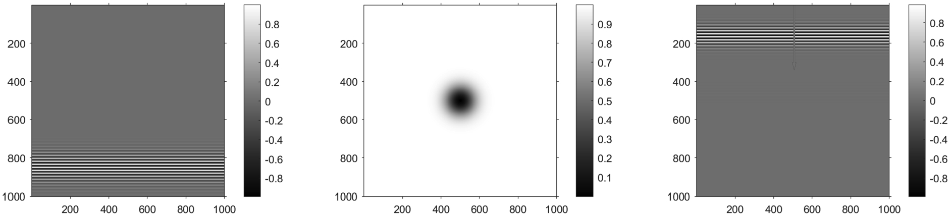
Figure 1 illustrates the setup. The probing wave $u_{in}^{R}$ (or its real part if we take its complex version $u_{in}^{C}$ ) at $t = 0$ is plotted on the left, and the Cauchy condition for its t-derivative is chosen so that it would propagate up. We take nonlinearities of the type $f (x, u) = α (x) F (u)$ (this particular form is not essential for the computations) with α a Gaussian plotted in the middle of the figure. Finally, the plot on the right is that of $Λ (u_{in}^{R})$ (or its real part), i.e., the solution at $t = T = 1.4$ . Since the effect of the nonlinearity is in the subprincipal term, it has no visible effect on that plot. Instead, in some of the figures below, we plot $u - u_{L}$ , where $u_{L}$ is the linear solution; i.e., we subtract the principal term. Then we plot a vertical cross-section of $u - u_{L}$ through the center in the direction shown: from top to bottom. We plot the top $1 / 3$ (approximately) of the cross-section, where $u - u_{L}$ is essentially supported.

Fig. 1.

The setup. All plots are of the real parts. Left: the initial condition. Center: the nonlinearity $α (x)$ . Right: the solution at $t = T$ .

6.1. Cubic nonlinearity, complex incident wave

We start with a complex probing wave.

Example 6.1 (Fig. 2).

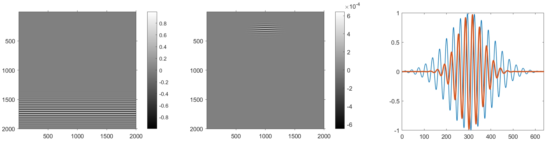
We take the nonlinearity to be $f = α (x) u^{3}$ as in Section 3.5. The subprincipal term in (1.6) then is $\begin{matrix} \frac{h}{2} e^{i (- T + x \cdot ω)} χ^{3} (- T + x_{∥}) X α (x_{⊥}, ω), where X α (x_{⊥}, ω) = \int α (x_{⊥} + s ω) d s . \end{matrix}$

Fig. 2.

$f (x, u) = α (x) u^{3}$ , $N = 2, 000$ , complex $u_{in}$ . All plots are of the real parts. Left: the initial condition. Center: the subprincipal term at $t = 1.4$ . Right: plot of a vertical cross section of the subprincipal term through the center (in red) and that of the linear solution (in blue).

In Fig. 2, we plot the real parts of the subprincipal term (in red) vs. the principal one; with the subprincipal term rescaled to have the same maximal amplitude, i.e., divided by $h (X α) / 2$ . We see that the subprincipal term decays faster away from the center because it has $χ^{3}$ as an envelope of the oscillations instead of χ. The two oscillations are shifted by $π / 2$ which is due to the $i = \sqrt{- 1}$ factor.

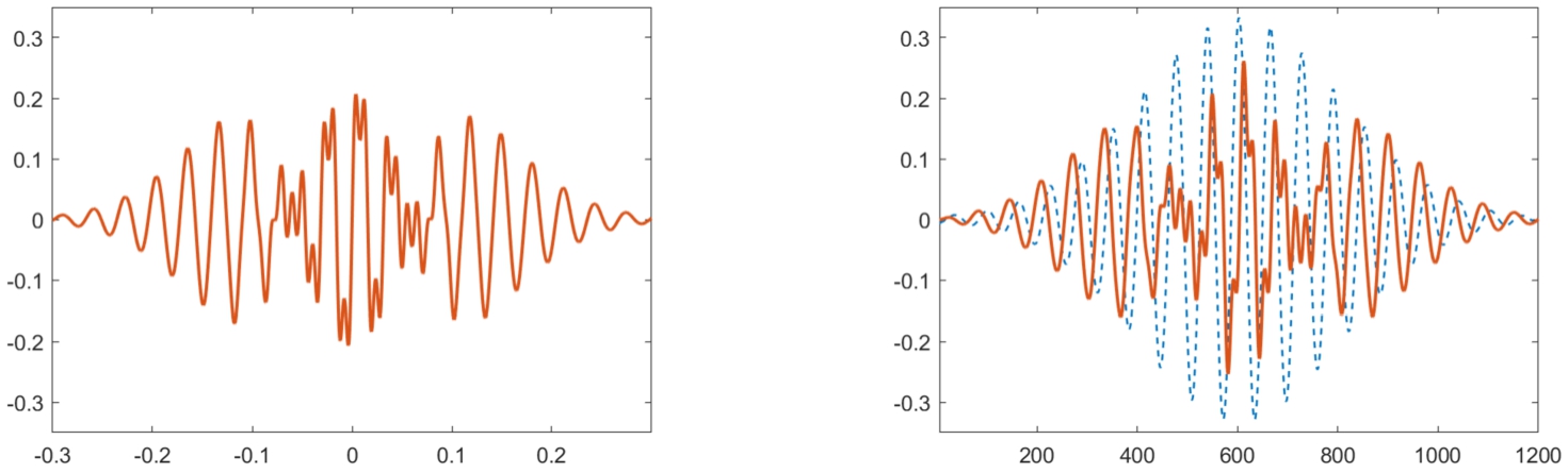
6.2. More general nonlinearities with separated variables, complex incident wave

Assume $f (x, u) = α (x) G (| u |^{2}) u$ . Then (1.6) takes the form $\begin{matrix} (6.1) & Λ (u_{in}) = e^{i ϕ / h} χ (ϕ) + i \frac{h}{2} e^{i ϕ / h} (X α) χ (ϕ) G (χ^{2} (ϕ)) + O (h^{2}), ϕ : = - T + x \cdot ω . \end{matrix}$ The envelope of the oscillations then is proportional to $(X α) χ (- T + x_{∥}) G (χ^{2} (- T + x_{∥}))$ .

Example 6.2 (Fig. 3).

We choose $F (u) : = G (| u |^{2}) u = 1.5 \sqrt{3} (1 - | u |^{2}) u$ . It has a maximum 1 on the interval $[0, 1]$ . Then we chose $χ (s) = exp (- s^{2} / 0.02)$ . A plot of the function $F \circ χ = G (χ^{2} (\cdot)) χ (\cdot)$ and $- F \circ χ$ are shown on Fig. 3, left. By (6.1), it must be the envelope of the oscillations of the subprincipal term and the computed profile in Fig. 3, right, confirms that. The curve in red is the subprincipal term divided by $h (X α) / 2$ as above.

Fig. 3.

$f (x, u) = α (x) 1.5 \sqrt{3} (1 - | u |^{2}) u$ , $N = 1, 000$ , complex $u_{in}$ . All plots are of the real parts. Left: the theoretical envelope $F \circ χ$ of the oscillations. Right: a plot of a vertical cross section of the subprincipal term through the center, rescaled (in red) and that of the linear solution (in blue).

The recovery of g then goes along the following lines. We fix $x_{∥}$ , which fixes $M : = χ (- T + x_{∥})$ . Then the subprincipal term in (6.1) recovers $F (M) X α (x_{⊥}, ω)$ . Knowing this for all ω recovers $F (M) α (x)$ . Now, varying $x_{∥}$ , we vary M on the range of χ, which recovers $F (M) α (x)$ . It is also worth noticing that the envelope of the oscillations in Fig. 3, right, is proportional to $F \circ χ$ , which recovers F, and therefore, f, up to a constant factor even without inverting the X-ray transform.

6.3. Nonlinearities with separated variables, a real incident wave

We assume a nonlinearity as in Section 6.2. Then $f (x, u) = α (x) F (u)$ by definition, where $F (u) = g (| u |^{2}) u$ . We have $\begin{matrix} (6.2) & γ_{m} (x, M) = α (x) {\tilde{γ}}_{m} (M), {\tilde{γ}}_{m} (M) : = \frac{4}{M π} \int_{0}^{1} [F (M q)] T_{m} (q) \frac{d q}{\sqrt{1 - q^{2}}} \end{matrix}$ see (1.8). By (1.10), (3.14), $\begin{matrix} (6.3) & X γ_{k} = (X α) {\tilde{γ}}_{m} (- T + x_{∥}) . \end{matrix}$ Then the subprincipal term in (3.13) takes the form $\begin{matrix} (6.4) & h X α (x_{⊥}) χ (- T + x_{∥}) \sum_{k ⩾ 1, odd} \frac{1}{2 k} sin \frac{k (- T + x_{∥})}{h} {\tilde{γ}}_{k} (χ (- T + x_{∥})) . \end{matrix}$

Assume now that F is a polynomial. Then $F (u) = \sum_{m ⩾ 1, odd} F_{m} u^{m}$ . There is a well known expansions of monomials $q^{m}$ into Chebyshev polynomials; and we can use that in (6.2). We will do this for polynomials F of degree five only. We have $\begin{matrix} q = T_{1} (q), q^{3} = \frac{1}{4} T_{3} (q) + \frac{3}{4} T_{1} (q), q^{5} = \frac{1}{16} T_{5} (q) + \frac{5}{16} T_{3} (q) + \frac{5}{8} T_{1} (q) . \end{matrix}$ Then $\begin{matrix} {\tilde{γ}}_{1} = F_{1} + \frac{3}{4} F_{3} M^{2} + \frac{5}{8} F_{5} M^{4}, {\tilde{γ}}_{3} = \frac{1}{4} F_{3} M^{2} + \frac{5}{16} F_{5} M^{4}, {\tilde{γ}}_{5} = \frac{1}{16} F_{5} M^{4} . \end{matrix}$ The subprincipal term then takes the form, see (6.4), $\begin{aligned} h (X α) M [\frac{1}{2} (F_{1} + \frac{3}{4} F_{3} M^{2} + \frac{5}{8} F_{5} M^{4}) sin \frac{ϕ}{h} \\ (6.5) & + \frac{1}{6} (\frac{1}{4} F_{3} M^{2} + \frac{5}{16} F_{5} M^{4}) sin \frac{3 ϕ}{h} + \frac{1}{10} \cdot \frac{1}{16} F_{5} M^{4} sin \frac{5 ϕ}{h}] . \end{aligned}$ In that case, we can easily demonstrate the two algorithms for recovery of the nonlinearity. To make things simple, assume that α is known. If we know (6.5) for a all M in some interval $[0, K]$ , then we can easily recover $F_{1}$ , $F_{2}$ and $F_{3}$ from the first harmonic in (6.5), which is proportional to ${\tilde{γ}}_{1}$ . On the other hand, if M is fixed, we can recover the three ${\tilde{γ}}_{k}$ , and then recover $F (M q)$ by its Chebyshev expansion.

Example 6.3 (cubic nonlinearity, Fig. 4).

In particular, if $F (u) = | u |^{2} u$ (equal to $u^{3}$ for u real), we get ${\tilde{γ}}_{1} = 3 M^{2} / 4$ , ${\tilde{γ}}_{3} = M^{2} / 4$ , all other zero, see (3.21); therefore, the subprincipal term is $\begin{matrix} (6.6) & h X α (x_{⊥}) χ^{3} (- T + x_{∥}) (\frac{3}{4} sin \frac{- T + x_{∥}}{h} + \frac{1}{24} sin \frac{3 (- T + x_{∥})}{h}) . \end{matrix}$

In Fig. 4, left, we plot a vertical cross-section of $u_{t = T}$ and that of the difference $(u - u_{L}) / (h X α)$ at $t = T$ . The theoretical maximum of that difference would be $3 / 4 + 1 / 24 \approx 0.79$ (modulo $O (h)$ because it would depend on the phase shift of the oscillations in (6.4) related to $x_{∥} = T$ maximizing χ there). This is in good agreement with the experimental plot.

Next to that plot, in Fig. 4, right, we plot the modulus of the Fourier transform of that difference on a log scale. We can see a peak at the incident frequency: the first (the carrier) harmonic, the third harmonic affecting the subprincipal term (and the lower order ones) and the fifth one affecting the lower order terms starting from the sub-subprincipal one.

Fig. 4.

$f (x, u) = α (x) u^{3}$ , $N = 2, 000$ , real $u_{in}$ . Left: a plot of a vertical cross section of $u - u_{L}$ (scaled) through the center (in red) and that of u (in blue). Right: the modulus of the Fourier transform on a log scale of it: the first, third harmonics dominate, and the fifth one is coming from the third order term.

Fig. 5.

$f (x, u) = α (x) (u - 1.9 u^{3})$ , $N = 4, 000$ , real $u_{in}$ . Left: a plot of the theoretical vertical cross section of $(u - u_{L}) / h$ . Right: the computed one vs. $0.33 u_{L}$ .

Example 6.4 (Fig. 5).

In the next example, we choose a polynomial of degree three in order to make the third harmonics not just measurable but also visible. We choose $F_{1} = 1$ , $F_{3} = - 1.9$ , i.e., $\begin{matrix} F (u) = u - 1.9 u^{3} . \end{matrix}$ The first term represents a linear potential $V = 1$ , actually. The coefficients are chosen so that ${\tilde{γ}}_{1} = 0$ for $M \approx 0.84$ , which would kill the first harmonic when $χ \approx 0.84$ (close to its peak $χ = 1$ ). We plot the theoretical profile of the subprincipal term divided by h, versus the computed one in Fig. 5. There is no perfect match because of numerical dispersion: higher frequencies travel slower. Still, one can see evidence of the third harmonics near the center part. The effect is much stronger and eclipses the first harmonic approximately where χ is closer to 0.84. The linear solution is plotted divided by 3.

Fig. 6.

$f (x, u) = α (x) u^{2}$ , $N = 2, 000$ , $t = T = 1.4$ . Left: $u - u_{L}$ , represents the computed zeroth harmonic up to $O (h)$ . Center: $u_{0, theor}^{(0)}$ , the theoretical zeroth harmonic up to $O (h)$ . Right: the difference of the two, representing the subprincipal term up to $O (h^{2})$ .

Fig. 7.

As in Fig. 6. Vertical profiles of $(u - u_{L}) / h$ , left, and $(u - u_{L} - u_{0, theor}^{(0)}) / h$ , right; both plotted against u (in blue).

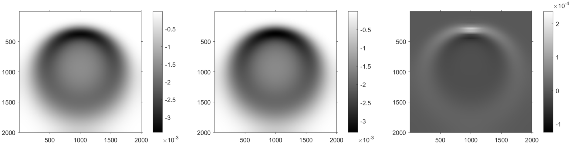
Example 6.5 (quadratic nonlinearity, Figs 6, 7).

Let $f (x, u) = α (x) u^{2}$ . We recall the analysis in Section 4.1. We compute a linear solution $u_{L}$ first, i.e., with $α = 0$ . It is equal to $u_{in}^{R}$ , of course, which also represents the first term in (4.1). Then we compute $u_{0, theor}^{(0)}$ as a numerical solution of (4.4). This would be the theoretical zeroth mode, up to a lower order term. Next, we compute u itself. The zeroth mode $u_{0}^{(0)}$ is relatively small since its size depends on χ as well (which has small “support” in our case), and it propagates in all directions; therefore it spreads. For this reason, we do not plot $u |_{t = T}$ ; it looks more or less as the unperturbed $u_{L} |_{t = T}$ in this case. In Fig. 6, we plot $u - u_{L}$ , $u_{0, theor}^{(0)}$ , and $u - u_{L} - u_{0, theor}^{(0)}$ at $t = T$ . According to (4.1), we should have $\begin{aligned} u - u_{L} = u_{0, theor}^{(0)} + O (h), \\ u - u_{L} - u_{0, theor}^{(0)} = h (- 2 (ℑ a_{1}^{(1)}) sin (ϕ / h) - 2 (ℑ a_{1}^{(2)}) sin (2 ϕ / h)) + O (h^{2}) . \end{aligned}$ Therefore, the first two plots should be very close. Indeed, they are, and in $u - u_{L}$ , we see a slight hint of the oscillations due to the subprincipal term. The third plot represents the difference $u - u_{L} - u_{0, theor}^{(0)}$ , and we see the oscillations. Note that the third plot is on a different scale – about 15 times smaller.

In Fig. 7, we plot vertical profiles of $(u - u_{L}) / h$ , left, and $(u - u_{L} - u_{0, theor}^{(0)}) / h$ , right. Even though $u_{0}^{(0)}$ is a principal order term, as mentioned above, it is much smaller than the leading cosine term but still larger than the harmonic frequencies in the subprincipal term. The red curve on the left is an approximation of $h^{- 1} u_{0}^{(0)}$ plus the subprincipal oscillatory terms. One can see the second harmonic mostly but $u_{0}^{(0)}$ dominates. With that low frequency wave subtracted (computed as a solution of (4.4)), we see, on the right, the second harmonic mostly. Numerical calculations, not shown, using the formula (4.6) to compute the theoretical amplitude of the second harmonic, agree very well with the plot in Fig. 7, right.

7. Remarks

In our main results, we do not impose assumptions on f guaranteeing existence and uniqueness of solutions of (1.1) for $t \in [0, T]$ with arbitrary, even smooth but not small data. We prove that (1.1) is solvable with the initial conditions (1.3), or its real part, for $h ≪ 1$ ; and that the solution is smooth. By Theorem A.1, this solution is unique in the class of the bounded solutions at least (then the bound $‖ u_{j} ‖_{L^{\infty}} ⩽ M$ in Theorem A.1 holds). We do not exclude a priori existence of other, unbounded solutions. If f satisfies the assumptions of Theorem A.4 however, such solutions do not exist.

The methods extend naturally to a wave equation of the type $u_{tt} - Δ_{g} u = 0$ related to a Riemannian metric or even to $Δ_{g}$ involving a magnetic and an electric potential, as long as there are no caustics. In fact, an electric potential term $Vu$ can be absorbed in the nonlinearity. Even Lorentzian wave operators can be treated. On the other hand, the inversion of the light ray transform on non-Minkowski manifolds is a more delicate problem.

One can pose the problem as a boundary value problem, in principle, on a cylinder $[0, T] \times \partial Ω$ , given a certain (non-linear) outgoing Dirichlet-to-Neumann map; where $Ω \subset R^{n}$ is a fixed domain. Under the assumption that the x-support of the nonlinearity is contained in Ω, a reduction from our formulation to such one and back is trivial. If we do not have the support assumption, we would have to deal with the boundary value problem for (1.1) first, a task we wanted to avoid for the purpose of this work. On the other hand, in authors’ view, the Dirichlet-to-Neumann map formulation for the wave equation is a bit artificial, while probing the medium with waves coming from outside at $t = 0$ and measuring them outside again, for $t = T$ is a more natural formulation.

The compactness of ${supp}_{x} f$ does not seem to be needed for the direct problem. It certainly simplifies the exposition though.

One can use probing waves with support localized near a point of the type $u_{in} = e^{i (- t + x \cdot ω)} ψ (x)$ (or its real part), $ψ \in C_{0}^{\infty}$ , at some initial moment, and an appropriate initial condition for $u_{t}$ , compare with (1.3) or (1.7). It was simpler to multiply (1.3) or (1.7) by a $C_{0}^{\infty}$ function of $x_{⊥}$ . Note that this localization would be h-independent, this would add more terms to the asymptotic expansion but it will not change the main idea.

We restrict the space dimension to $n = 2$ or $n = 3$ because the stability estimate (A.17) in Theorem A.3 has a short proof then.

8. Discussion

There has been an increased interest in inverse problems for non-linear hyperbolic equations recently. The pioneering works [22] and [25] suggested the higher order linearization idea mentioned in the introduction: send a wave $u_{0} = ε_{1} u_{1} + ε_{2} u_{2} + ε_{3} u_{3} + ε_{4} u_{4}$ , where $u_{j}$ are chosen so that they carry conormal singularities colliding at a chosen in advance point in time-space. This collision creates a point source through non-linear interaction which emits a spherical wave in the $ε_{1} ε_{2} ε_{3} ε_{4}$ term as all $ε_{j} \to 0$ . This term must be separated from all other, and its (weak) singularity has to be measured to recover the nonlinearity at that point in time-space. This method has been used in other papers, see, e.g., [11–13,23–25,35]. In [29], three such waves are sent and each one is a (linear) Gaussian beam.

In [31], we proposed a different direction: send a wave which propagates in the so-called weakly non-linear regime. It has an amplitude $h^{- 1 / 2}$ and a wavelength $\sim h$ . The math theory of the weakly non-linear propagation has been developed in [3,4,15,16,26,27,30] (and other works), and it is known in the physics literature as well. Most of these work are on fist order non-linear systems. The waves there have the asymptotic behavior $u \sim h^{p} U (ϕ / h, t, x)$ , where p is chosen so that the nonlinearity does not affect the eikonal equation for ϕ but affects the leading transport equation. In the equation $□ u + α | u |^{J - 1} u = 0$ , for example, one gets $p = - 1 / (J - 1)$ ; in particular $p = - 1 / 2$ for a cubic nonlinearity. The first transport equation is a non-linear ODE, or a system of such; and we showed that its solution induces a phase shift proportional to the X-ray transform of α, which allows us to recover α. The essential difference of the approach in [31] with the higher order linearization method is that we propagate waves in an actual non-linear regime; and the signal carrying the useful information is the principal one instead of a signal of order $- 4$ .

We want to emphasize that none of the approaches above can recover general nonlinearities $f (x, u)$ away from the two extremes $u \sim 0$ and $u \sim \infty$ . The first approach relies on asymptotically small waves having the potential to recover the Taylor expansion of $f (x, u)$ about $u = 0$ . In fact, this is what is done in [25], starting with terms of order 4 and higher. The second one requires an asymptotic expansion of f w.r.t. u when $u \to \infty$ (at least as a leading term), requires strong assumptions on f for solvability, and one would expect that it has the potential to reliably recover that asymptotic behavior only, see also [31].

This brings us to the main idea of this paper: use solutions for which $p = 0$ above, i.e., $u \sim 1$ . Then the nonlinearity affects the subprincipal term but not the principal one of high-frequency solutions. We would expect to need high-frequency solutions in order to get good resolution.

The geometric optics analysis in the papers cited above, see, e.g., [26] for a survey, when applied to the wave equation, is not restricted to polynomial nonlinearities only (they are all x-independent though) but in effect, they always rely in the Taylor expansion of f about $u = 0$ . In many of them, the small parameter h (called there ε) is a part of the PDE as well, for example the derivatives could be replaced by their semi-classical ones $h \partial_{t}$ , $h \partial_{x}$ , or similar. This is equivalent to rescaling time and/or space. This would change the value of p above for which the propagation is in the weakly non-linear regime, and it could make it $p = 0$ . This happens for the PDE $h □ u + α | u |^{J - 1} u = 0$ , for example, which is obtained from its h-independent version after the scaling $t^{'} = h^{1 / 2} t$ , $x^{'} = h^{1 / 2} x$ . We are studying h-independent PDEs however over h-independent domains in time-space.

We also want to mention the method of linearization near a non-zero solution initiated by Isakov. In [21], a uniqueness result is proven when there are also internal measurements at $t = T$ as well.

Footnotes

Acknowledgements

The authors would like to thank the anonymous referee for making valuable suggestions which helped us improve the exposition.

The first author is partly supported by the Simons Foundation grants #349507 and #848410. The second author is partly supported by the NSF Grants DMS-1900475 and DMS-2154489.

Properties of solutions of semilinear wave equations

We prove some results for semilinear wave equations which are known to experts, see [17,18,33], but their proofs do not seem to be readily available and so we include them here for completeness and because they are elementary. We should also mention that part of this discussion, including a different version of Theorem A.1, is contained in [14, Ch. 6],

Let $g = \sum_{j, k = 1}^{n} g_{j k} (x) d x_{i} d x_{k}$ be a $C^{\infty}$ Riemannian metric in $R^{n}$ , $n ⩾ 2$ , such that $g_{j k} (x) = δ_{j k}$ if $| x | ⩾ R$ , for some $R > 0$ , and let $Δ_{g}$ be the corresponding (negative) Laplacian: $\begin{matrix} Δ_{g} = \frac{1}{\sqrt{| g (x) |}} \partial_{x_{j}} \sqrt{| g (x) |} g^{j k} (x) \partial_{x_{k}}, | g (x) | = det (g_{j k} (x)), and [g^{j k} (x)] = {[g_{j k} (x)]}^{- 1} . \end{matrix}$

We start by recalling an energy estimate for solutions of the linear wave equation: If $u (t, x)$ satisfies $\begin{aligned} u_{tt} - Δ_{g} u = G (t, x), \\ u (0, x) = φ (x), u_{t} (0, x) = ψ (x), \end{aligned}$ we have $\begin{matrix} u (t) = cos (t \sqrt{- Δ_{g}}) φ + t sinc (t \sqrt{- Δ_{g}}) ψ + \int_{0}^{t} (t - s) sinc ((t - s) \sqrt{- Δ_{g}})) G (s) d s, \end{matrix}$ where $sinc (t) = sin (t) / t$ , and we suppressed the dependence on x. Then for any $T > 0$ , and $s ⩾ 0$ , $\begin{aligned} sup_{[0, T]} {‖ u (t, \cdot) ‖}_{H^{s + 1} (R^{n})} + sup_{[0, T]} {‖ \partial_{t} u (t, \cdot) ‖}_{H^{s} (R^{n})} ⩽ C T E_{s + 1} (0), \\ (A.1) & where E_{s + 1} (0) = ‖ φ ‖_{H^{s + 1} (R^{n})} + ‖ ψ ‖_{H^{s} (R^{n})} + \int_{0}^{T} {‖ G (t, \cdot) ‖}_{H^{s} (R^{n})} d t, \end{aligned}$ provided the right hand side is finite.

We recall that a particular case of Gronwall’s inequality states that if f and g are continuous functions on $[0, T]$ , and $\begin{matrix} (A.2) & \begin{array}{r} if f (t) ⩽ g (t) + C \int_{0}^{t} f (s) d s, then for t \in [0, T], then f (t) ⩽ C_{1} g (t) . \end{array} \end{matrix}$

References

A.S.

Barreto,

Uhlmann and

Wang, Inverse scattering for critical semilinear wave equations, 2020, arXiv:2003.03822.

Brezis and

Mironescu, Gagliardo–Nirenberg, composition and products in fractional Sobolev spaces, J. Evol. Equ. 1(4) (2001), 387–404, Dedicated to the memory of Tosio Kato. doi:10.1007/PL00001378.

Donnat and

Rauch, Dispersive nonlinear geometric optics, J. Math. Phys. 38(3) (1997), 1484–1523. doi:10.1063/1.531905.

Dumas, About nonlinear geometric optics, Bol. Soc. Esp. Mat. Apl. SeMA 35 (2006), 7–41.

Eptaminitakis and

Stefanov, Weakly nonlinear geometric optics for the Westervelt equation and recovery of the nonlinearity, 2022, arXiv:2208.13945.

Fiorenza,

M.R.

Formica,

Roskovec and

Soudsky, Detailed proof of classical Gagliardo–Nirenberg interpolation inequality with historical remarks.

Ginibre and

Velo, Generalized Strichartz inequalities for the wave equation, J. Funct. Anal. 133(1) (1995), 50–68. doi:10.1006/jfan.1995.1119.

Gorenflo and

Vessella, Abel Integral Equations: Analysis and Applications, Lecture Notes in Mathematics, Vol. 1461, Springer-Verlag, Berlin, 1991.

M.G.

Grillakis, Regularity and asymptotic behaviour of the wave equation with a critical nonlinearity, Ann. of Math. (2) 132(3) (1990), 485–509. doi:10.2307/1971427.

10.

Guès, Développement asymptotique de solutions exactes de systèmes hyperboliques quasilinéaires, Asymptotic Anal. 6(3) (1993), 241–269. doi:10.3233/ASY-1993-6303.

11.

Hintz and

Uhlmann, Reconstruction of Lorentzian manifolds from boundary light observation sets, Int. Math. Res. Not. IMRN 22 (2019), 6949–6987. doi:10.1093/imrn/rnx320.

12.

Hintz,

Uhlmann and

Zhai, An inverse boundary value problem for a semilinear wave equation on Lorentzian manifolds, International Mathematics Research Notices 5 (2021).

13.

Hintz,

Uhlmann and

Zhai, The Dirichlet-to-Neumann map for a semilinear wave equation on Lorentzian manifolds, 2021, arXiv:2103.08110.

14.

Hörmander, Lectures on Nonlinear Hyperbolic Differential Equations, Mathématiques & Applications (Berlin) [Mathematics & Applications], Vol. 26, Springer-Verlag, Berlin, 1997.

15.

J.-L.

Joly,

Métivier and

Rauch, Coherent and focusing multidimensional nonlinear geometric optics, Ann. Sci. École Norm. Sup. (4) 28(1) (1995), 51–113. doi:10.24033/asens.1709.

16.

J.-L.

Joly and

Rauch, Justification of multidimensional single phase semilinear geometric optics, Trans. Amer. Math. Soc. 330(2) (1992), 599–623. doi:10.1090/S0002-9947-1992-1073774-7.

17.

L.V.

Kapitanskii, The Cauchy problem for the semilinear wave equation. II, Zap. Nauchn. Sem. Leningrad. Otdel. Mat. Inst. Steklov. (LOMI) 182 (1990), 38–85. (Kraev. Zadachi Mat. Fiz. i Smezh. Voprosy Teor. Funktsii. 21), 171.

18.

L.V.

Kapitanskii, The Cauchy problem for the semilinear wave equation. III, Zap. Nauchn. Sem. Leningrad. Otdel. Mat. Inst. Steklov. (LOMI) 181 (1990), 24–64. (Differentsial’naya Geom. Gruppy Li i Mekh. 11), 186.

19.

Kato and

Ponce, Commutator estimates and the Euler and Navier–Stokes equations, Comm. Pure Appl. Math. 41(7) (1988), 891–907. doi:10.1002/cpa.3160410704.

20.

J.B.

Keller, On solutions of nonlinear wave equations, Comm. Pure Appl. Math. 10 (1957), 523–530. doi:10.1002/cpa.3160100404.

21.

Kian, On the determination of nonlinear terms appearing in semilinear hyperbolic equations, Journal of the London Mathematical Society.

22.

Kurylev,

Lassas and

Uhlmann, Inverse problems for Lorentzian manifolds and non-linear hyperbolic equations, Invent. Math. 212(3) (2018), 781–857. doi:10.1007/s00222-017-0780-y.

23.

Lassas,

Liimatainen,

Potenciano-Machado and

Tyni, Uniqueness and stability of an inverse problem for a semi-linear wave equation, 2020, arXiv preprint arXiv:2006.13193.

24.

Lassas,

Uhlmann and

Wang, Determination of vacuum space-times from the Einstein–Maxwell equations, 2017, arXiv:1703.10704.

25.

Lassas,

Uhlmann and

Wang, Inverse problems for semilinear wave equations on Lorentzian manifolds, Comm. Math. Phys. 360(2) (2018), 555–609. doi:10.1007/s00220-018-3135-7.

26.

Métivier, The mathematics of nonlinear optics, in: Handbook of Differential Equations: Evolutionary Equations, Handb. Differ. Equ., Vol. V, Elsevier/North-Holland, Amsterdam, 2009, pp. 169–313. doi:10.1016/S1874-5717(08)00210-7.

27.

Métivier,

J.-L.

Joly and

Rauch, Recent results in non-linear geometric optics, in: Hyperbolic Problems: Theory, Numerics, Applications, Vol. II (Zürich, 1998), Internat. Ser. Numer. Math., Vol. 130, Birkhäuser, Basel, 1999, pp. 723–736. doi:10.1007/978-3-0348-8724-3_23.

28.

Meyer, Remarques sur un théorème de J.-M. Bony, Rend. Circ. Mat. Palermo (2) (suppl. 1) (1981), 1–20.

29.

Oksanen,

Salo,

Stefanov and

Uhlmann, Inverse problems for real principal type operators, 2020, arXiv preprint arXiv:2001.07599.

30.

Rauch, Hyperbolic Partial Differential Equations and Geometric Optics, Graduate Studies in Mathematics, Vol. 133, American Mathematical Society, Providence, RI, 2012.

31.

Sá Barreto and

Stefanov, Recovery of a cubic non-linearity in the wave equation in the weakly non-linear regime, Comm. Math. Phys. 392(1) (2022), 25–53. doi:10.1007/s00220-022-04359-0.

32.

Shatah and

Struwe, Regularity results for nonlinear wave equations, Ann. of Math. (2) 138(3) (1993), 503–518. doi:10.2307/2946554.

33.

Shatah and

Struwe, Well-posedness in the energy space for semilinear wave equations with critical growth, Internat. Math. Res. Notices 7 (1994).

34.

Stefanov, Support theorems for the light ray transform on analytic Lorentzian manifolds, Proc. Amer. Math. Soc. 145(3) (2017), 1259–1274. doi:10.1090/proc/13117.

35.

Uhlmann and

Zhang, Inverse boundary value problems for wave equations with quadratic nonlinearities, J. Differential Equations 309 (2022), 558–607. doi:10.1016/j.jde.2021.11.033.