On a biharmonic coupled system with non-standard nonlinearity: Existence,blow up and numerics

Abstract

In this paper, we consider a coupled system of two biharmonic equations with damping and source terms of variable-exponent nonlinearities, supplemented with initial and mixed boundary conditions. We establish an existence and uniqueness result of a weak solution, under suitable assumptions on the variable exponents. Then, we show that solutions with negative-initial energy blow up in finite time. To illustrate our theoritical findings, we present two numerical examples.

Keywords

Biharmonic operator Existence Blow up Coupled system Variable exponent Weak solution

1. Introduction

In this work, we study the following biharmonic (or Petrovsky) coupled system with initial and boundary conditions: $\begin{matrix} (1.1) & \{\begin{array}{ll} u_{t t} + Δ^{2} u + | u_{t} |^{m (x) - 2} u_{t} = f_{1} (u, v) & in Ω \times (0, T), \\ v_{t t} + Δ^{2} v + | v_{t} |^{r (x) - 2} v_{t} = f_{2} (u, v) & in Ω \times (0, T), \\ u = v = 0 & on \partial Ω \times (0, T), \\ \frac{\partial u}{\partial η} = \frac{\partial v}{\partial η} = 0 & on \partial Ω \times (0, T), \\ (u (0), v (0)) = (u_{0}, v_{0}) and (u_{t} (0), v_{t} (0)) = (u_{1}, v_{1}) & in Ω \times Ω, \end{array} \end{matrix}$ where $T > 0, Ω$ is a smooth and bounded domain of $R^{n}, (n = \overline{1, 6})$ , the exponents m and r are continuous functions on $\overline{Ω}$ satisfying some conditions to be specified later, $\frac{\partial u}{\partial η}$ and $\frac{\partial v}{\partial η}$ denote the external normal derivatives of u and v, respectively, on the boundary $\partial Ω$ and the coupling terms $f_{1}$ and $f_{2}$ are given as follows: for all $x \in \overline{Ω}$ and $(u, v) \in R^{2}$ , $\begin{matrix} (1.2) & f_{1} (x, u, v) = \frac{\partial}{\partial u} F (x, u, v) and f_{2} (x, u, v) = \frac{\partial}{\partial v} F (x, u, v), \end{matrix}$ with $\begin{matrix} (1.3) & F (x, u, v) = a | u + v |^{p (x) + 1} + 2 b | u v |^{\frac{p (x) + 1}{2}}, \end{matrix}$ where $a, b > 0$ are two positive constants and p is a given continuous function on $\overline{Ω}$ satisfying the condition $(H .3)$ bellow.

The fourth single-order nonlinear equations arise in various physical phenomena such as the study of travelling waves in suspnssion bridges [22], micro-electro mechanical systems [34], bending behaviour of a thin elastic rectangular plate [37], geometric and functional design [9], radar imaging [4],…, etc.

Other physical phenomena like flows of electro-rheological fluids, fluids with temperature dependent viscocity, filtration processes through a porous media, image processing and thermorheological fluids give rise to mathematical models of hyperbolic, parabolic and biharmonic equations with variable exponents of nonlinearity. See [6,7,35] for more details.

Recently, the hyperbolic equations with nonlinearties of variable exponents type had received a considerable amount of attention. Treating this class of problems, the researchers in [17,26,27,29,30,33] investigated the local existence and blow up of solutions, whereas in [14,18,23,32,38], they estabilshed several uniform estimates of decay rates of the solution energy.

Concerning coupled systems of wave equations in the variable-exponents case, we have only few works. In [10], Bouhoufani and Hamchi obtained the global existence of a weak solution and established decay rates of the solution in a bounded domain. Messaoudi et al. [26] studied the same system and proved a theorem of existence and uniqueness of a weak solution, established a blow-up result for certain solutions with positive-initial energy and gave some numerical applications for their theoritical resuls. Also, Messaoudi and Talahmeh [28] treated a system of hyperbolic equations with variable exponents in the damping and source terms, and established a blow-up result for solutions with negative initial energy. In [29], Messaoudi et al. considered the following system $\begin{aligned} (1.4) & \{\begin{array}{ll} u_{t t} - Δ u + | u_{t} |^{m (x) - 2} u_{t} + f_{1} (u, v) = 0 & in Ω \times (0, T), \\ v_{t t} - Δ v + | v_{t} |^{r (x) - 2} v_{t} + f_{2} (u, v) = 0 & in Ω \times (0, T), \end{array} \end{aligned}$ with initial and Dirichlet-boundary conditions (here $f_{1}$ and $f_{2}$ are the coupling terms introduced in (1.2)). The authors proved the existence of global solutions, obtained explicit decay rate estimates, under suitable assumptions on the variable exponents $m, r$ and p and presented some numrical tests. Recently, Bouhoufani et al. [11] treated a similar system to $(1.4)$ , where $\begin{matrix} f_{1} (u, v) = | u |^{p (x) - 2} u | v |^{p (x)} and f_{2} (u, v) = | v |^{p (x) - 2} v | u |^{p (x)} \end{matrix}$ and the damping term, in each equation, is modilated by a time-dependent coefficients $α (t)$ and $β (t)$ . They established decay rate results, under appropriate assumptions on the coefficient functions and the variable exponents and illustrated their results by some examples and numerical tests.

For equations and systems with biharmonic operator and constant exponents of nonlinearity, we mention the work by Komornik [20], in which he proved the well-posedness for a Petrovsky equation, by using the nonlinear semigroup theory, and established the energy decay estimates for weak solutions. Guesmia [15] used the same approach to obtain a global existence, uniqueness and regularity results for a Petrovsky equation, in a more general setting. He, established decay estimates of weak, as well as strong solutions, under suitable conditions on the damping term. In [16], the same author proved the well-posedness and uniform stabilisation for a damped nonlinear coupled system of two Petrovsky equations, under appropriate assumptions. After that, Assila and Guesmia [1] considered the following problem $\begin{array}{r} \{\begin{array}{ll} u_{t t} + k_{1} Δ^{2} u + k_{2} Δ^{2} u_{t} + Δ g (Δ u) = 0 & in Ω \times R^{+}, \\ u = \partial_{η} u = 0 & on \partial Ω \times R^{+}, \\ u (0) = u_{0} and u_{t} (0) = u_{1} & on Ω, \end{array} \end{array}$ where $k_{1}$ and $k_{2}$ are two positive constants, and g is a $C^{2}$ -class real valued function. By invoking an important Lemma of Komornik [19], they showed that the solution energy decays exponentially. The well-posedness of this type of problems has been studied in many papers; the reader can see, for example, the work by Banks et al. [8]. For the Petrovsky equation with nonlinear source term, we have the work of Messaoudi [31], in which he studied the problem: $\begin{array}{r} \{\begin{array}{ll} u_{t t} + Δ^{2} u + a u_{t} | u_{t} |^{m - 2} = b u | u |^{ρ - 2} & in Ω \times R^{+}, \\ u = \partial_{η} u = 0 & on \partial Ω \times R^{+}, \\ u (0) = u_{0} and u_{t} (0) = u_{1} & on Ω, \end{array} \end{array}$ where a and b are positive constants and $m > 2$ . He obtained an existence result and showed that the solution blows up, in finite time, if $m < p$ and exists globally otherwise.

Very recently, Antontsev and al. [5] studied the following Petrovsky equation $\begin{aligned} (1.5) & u_{t t} + Δ^{2} u - Δ u_{t} + | u_{t} |^{m (x) - 2} u_{t} = | u |^{p (x) - 2} u . \end{aligned}$ They proved the existence of local weak solutions by using the Banach fixed-point theorem, and gave a blow-up result for negative-initial-energy solutions, under suitable assumptions. In [24], Liao and Tan treated a similar system with $M (‖ \nabla u ‖_{2}^{2}) Δ u$ in the left-hand side of the equation (1.5), where $M (s) = a + b s^{γ}$ is a positive $C^{1}$ -function, $a > 0, b > 0, γ ⩾ 1$ , and $m, p$ are given measurable functions. The upper and lower bounds of the blow-up time, as well as some uniform decay rates have been established.

To the best of our knowledge, the Petrovsky (or biharmonic) coupled system with variable exponents of nonlinearty given by (1.2) and (1.3), has never been studied. Our aim in this work is to prove the existence and uniqueness of a weak solution to the Petrovsky system (1.1), by using the Faedo–Galerkin method, together with a fixed-point principle. We also establish a blow-up result for negative-initial-energy solutions, under appropriate conditions on the variable exponents. We note here that the well-posedness is established only for $n ⩽ 6$ . For dimensions higher than 6, the problem remains open, see Remark 3.4 below.

The paper is devided into three sections, in addition to the introduction. In Section 2, we present some notations, definitions and important properties and tools of the variable-exponent Lebesgue and Sobolev spaces. We also introduce our assumptions. Section 3 is devoted to the statement and proof of the well-posedness. Our blow-up result will be given in Section 4. Finally, some numerical tests to verify the finite time blow-up result, are presented in Section 5.

2. Preliminaries

In this section, we define the variable-exponent Lebesgue and Sobolev spaces and, then, present some of their propereties and facts. For more details, see [7,12,21].

Let $q : Ω ⟶ [1, \infty)$ be a measurable function. We define the Lebesgue space with a variable exponent by $\begin{matrix} L^{q (.)} (Ω) = {f : Ω ⟶ R measurable in Ω : ϱ_{q (.)} (λ f) < + \infty, for some λ > 0}, \end{matrix}$ where $\begin{matrix} ϱ_{q (.)} (f) = \int_{Ω} {| f (x) |}^{q (x)} d x . \end{matrix}$ $L^{q (.)} (Ω)$ is a Banach space with respect to the following Luxembourg-type norm $\begin{matrix} ‖ f ‖_{q (.)} : = inf {λ > 0 : \int_{Ω} {| \frac{f (x)}{λ} |}^{q (x)} d x ⩽ 1} . \end{matrix}$ Let $k \in N$ . We define the variable exponent Sobolev space $W^{k, p (.)} (Ω)$ as follows: $\begin{matrix} W^{k, q (.)} (Ω) = {u \in L^{q (.)} (Ω) : \partial^{| α |} u \in L^{q (.)} (Ω), with | α | ⩽ k} . \end{matrix}$ $W^{k, q (.)} (Ω)$ is a Banach space equipped with the following norm $\begin{matrix} ‖ u ‖_{W^{k, q (.)} (Ω)} : = \sum_{0 ⩽ | α | ⩽ k} ‖ \partial_{α} u ‖_{q (.)}, \end{matrix}$ where $| α | = α_{1} + \dots + α_{n}$ .

Lemma 2.1.
(Young’s Inequality [ 7 , 21 ])Let $r, q, s ⩾ 1$ be measurable functions defined on Ω, such that $\begin{matrix} \frac{1}{s (y)} = \frac{1}{r (y)} + \frac{1}{q (y)}, for a.e. y \in Ω . \end{matrix}$ Then, for all $a, b ⩾ 0$ , we have $\begin{matrix} \frac{{(a b)}^{s (.)}}{s (.)} ⩽ \frac{{(a)}^{r (.)}}{r (.)} + \frac{{(b)}^{q (.)}}{q (.)} . \end{matrix}$
Lemma 2.2.
(Hölder’s Inequality [ 7 , 21 ]) Let $r, q, s : Ω ⟶ [1, \infty)$ be measurable functions, such that $\begin{matrix} \frac{1}{s (y)} = \frac{1}{r (y)} + \frac{1}{q (y)}, for a.e. y \in Ω . \end{matrix}$ If $f \in L^{r (.)} (Ω)$ and $g \in L^{q (.)} (Ω)$ , then $f g \in L^{s (.)} (Ω)$ , with $\begin{matrix} ‖ f g ‖_{s (.)} ⩽ 2 ‖ f ‖_{r (.)} ‖ g ‖_{q (.)} . \end{matrix}$
Lemma 2.3 ([7,21]).

If $1 < q^{-} ⩽ q (x) ⩽ q^{+} < + \infty$ holds then, for any $f \in L^{q (.)} (Ω)$ , $\begin{matrix} min {‖ f ‖_{q (.)}^{q^{-}}, ‖ f ‖_{q (.)}^{q^{+}}} ⩽ ϱ_{q (.)} (f) ⩽ max {‖ f ‖_{q (.)}^{q^{-}}, ‖ f ‖_{q (.)}^{q^{+}}}, \end{matrix}$ where $\begin{matrix} q^{-} = ess inf_{x \in Ω} q (x) and q^{+} = ess sup_{x \in Ω} q (x) . \end{matrix}$

Lemma 2.4 ([21]).

If $q^{+} < + \infty$ , then $C_{0}^{\infty} (Ω)$ is dense in $L^{q (.)} (Ω)$ .

Definition 2.5.
We say that a function $q : Ω ⟶ R$ is log-Hölder continuous on Ω, if there exists a constant $θ > 0$ such that for all $0 < δ < 1$ , we have $\begin{matrix} | q (x) - q (y) | ⩽ - \frac{θ}{log | x - y |}, for a.e. x, y \in Ω, with | x - y | < δ . \end{matrix}$
Remark 2.6.
The log-Hölder continuity condition on q can be replaced by $q \in C (\overline{Ω})$ , if Ω is bounded.
Definition 2.7.
The closure of the set of $W^{k, q (.)} (Ω)$ -functions with compact support in $W^{k, q (.)} (Ω)$ is the Sobolev space $W_{0}^{k, q (.)} (Ω)$ “with zero boundary trace”, i.e., $\begin{matrix} W_{0}^{k, q (.)} (Ω) = {\overline{u \in W^{k, q (.)} (Ω) : u = u χ_{K} for a compact K \subset Ω}} . \end{matrix}$ Furtheremore, we denote by $H_{0}^{k, q (.)} (Ω)$ the closure of $C_{0}^{\infty} (Ω)$ in $W^{k, q (.)} (Ω)$ and by $W^{- k, q^{'} (.)} (Ω)$ the dual space of $W_{0}^{k, q (.)} (Ω)$ , in the same way as the usual Sobolev spaces, where $\frac{1}{q (.)} + \frac{1}{q^{'} (.)} = 1$ .
Lemma 2.8.
(Embedding Property [ 12 ]) Let $q : Ω ⟶ [1, \infty)$ be a measurable function and $k ⩾ 1$ be an integer. Suppose that r is a log-Hölder continuous function on Ω, such that, for all $x \in Ω$ , we have $\begin{matrix} \{\begin{array}{ll} k ⩽ q^{-} ⩽ q (x) ⩽ q^{+} < \frac{n r (x)}{n - k r (x)}, & if r^{+} < \frac{n}{k}, \\ k ⩽ q^{-} ⩽ q^{+} < \infty, & if r^{+} ⩾ \frac{n}{k} . \end{array} \end{matrix}$ Then, the embedding $W_{0}^{k, r (.)} (Ω) ↪ L^{q (.)} (Ω)$ is continuous and compact.

Throughout this paper, we denote by $V$ the following space $\begin{matrix} V = {u \in H^{2} (Ω) : u = \frac{\partial u}{\partial η} = 0 on \partial Ω} = H_{0}^{2} (Ω) . \end{matrix}$ So, $V$ is a separable Hilbert space endowed with the inner product and norm, respectively, $\begin{matrix} {(u, v)}_{V} = \int_{Ω} Δ u Δ v d x and ‖ u ‖_{V} = ‖ Δ u ‖_{2}, \end{matrix}$ where $‖ Δ u ‖_{k} = ‖ Δ u ‖_{L^{k} (Ω)}$ .

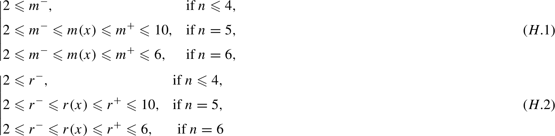
Now, we present our assumptions on the variable exponents $m, r$ and p, that will be used in the sequel. So, for all $x \in \overline{Ω}$ , we assume that

and

where $\begin{aligned} m^{-} = inf_{x \in \overline{Ω}} m (x), m^{+} = sup_{x \in \overline{Ω}} m (x), \\ r^{-} = inf_{x \in \overline{Ω}} r (x), r^{+} = sup_{x \in \overline{Ω}} r (x), \\ p^{-} = inf_{x \in \overline{Ω}} p (x) and p^{+} = sup_{x \in \overline{Ω}} p (x) . \end{aligned}$
3. Existence of weak solution

Before starting our study, we introduce the definition of a weak solution for system $(1.1)$ . We multiply the first equation in $(1.1)$ by $Φ \in C_{0}^{\infty} (Ω)$ and the second equation by $Ψ \in C_{0}^{\infty} (Ω)$ , integrate each result over Ω, and use Green’s formula and the boundary conditions to obtain the following:

Definition 3.1.
(Weak Solution of ( 1.1 ))

Let $(u_{0}, u_{1}), (v_{0}, v_{1}) \in V \times L^{2} (Ω)$ . Any pair of functions $(u, v)$ , such that

is called a weak solution of $(1.1)$ on $[0, T)$ , if $\begin{matrix} \{\begin{array}{l} \frac{d}{d t} \int_{Ω} u_{t} Φ d x + \int_{Ω} Δ u Δ Φ d x + \int_{Ω} | u_{t} |^{m (x) - 2} u_{t} Φ d x \\ = \int_{Ω} f_{1} Φ d x, \\ \frac{d}{d t} \int_{Ω} v_{t} Ψ d x + \int_{Ω} Δ v Δ Ψ d x + \int_{Ω} | v_{t} |^{r (x) - 2} u_{t} Ψ d x \\ = \int_{Ω} f_{2} Ψ d x, \\ u (0) = u_{0}, u_{t} (0) = u_{1}, v (0) = v_{0}, v_{t} (0) = v_{1}, \end{array} \end{matrix}$ for a.e. $t \in (0, T)$ and all test functions $Φ, Ψ \in V$ .

Note that $C_{0}^{\infty} (Ω)$ is dense in $V$ and $V \subset L^{m (.)} (Ω) \cap L^{r (.)} (Ω)$ .

In order to establish an existence result of a local weak solution for system $(1.1)$ , we, first, consider the following initial-boundary-value problem:

for given $f, g \in L^{2} (Ω \times (0, T))$ and $T > 0$ .

We have the following theorem of existence and uniqueness for problem $(S)$ .
Theorem 3.2.
Let $n = \overline{1, 6}$ and $(u_{0}, u_{1}), (v_{0}, v_{1}) \in V \times L^{2} (Ω)$ . Assume that $(H .1)$ – $(H .2)$ hold. Then, the problem $(S)$ admits a unique weak solution on $[0, T)$ , in the sense of Definition $3.1$ , having the regularity $(3.1)$ .
Proof.
EXISTENCE:

To prove the existence of the solution for $(S)$ , we use the Faedo–Galerkin method. It will be carried out in the following steps.

Approximate Problem. Consider ${ω_{j}}_{j = 1}^{\infty}$ an orthonormal basis of $V$ and define, for all $k ⩾ 1$ , $(u^{k}, v^{k})$ a sequence in $V_{k} = span {ω_{1}, ω_{2}, \dots, ω_{k}} \subset V$ , given by $\begin{matrix} u^{k} (x, t) = Σ_{j = 1}^{k} a_{j} (t) ω_{j} (x) and v^{k} (t) = Σ_{j = 1}^{k} b_{j} (t) ω_{j} (x) \end{matrix}$ for all $x \in Ω$ and $t \in (0, T)$ and solves the following approximate problem:

for all $j = 1, 2, \dots, k$ , with

such that

For any $k ⩾ 1$ , problem $(S_{k})$ generates a system of k nonlinear ordinary differential equations. The ODE standard existence theory assures the existence of a unique $(a_{j}, b_{j})$ in $C^{2} ([0, T_{k})), j = 1, 2, \dots, k$ , $0 < T_{k} ⩽ T$ , such that $(u^{k}, v^{k})$ is a solution of $(S_{k})$ .

Next, we have to show, by a priory estimates, that $T_{k} = T, \forall k ⩾ 1$ .

A Priori Estimates. Multiplying ${(S_{k})}_{1}$ and ${(S_{k})}_{2}$ by $a_{j}^{'} (t)$ and $b_{j}^{'} (t)$ , respectively, and then summing each result over $j = \overline{1, k}$ , we obtain, for all $0 < t ⩽ T_{k}$ , $\begin{aligned} \frac{1}{2} \frac{d}{d t} [\int_{Ω} ({| u_{t}^{k} (x, t) |}^{2} + {(Δ u^{k})}^{2} (x, t)) d x] + \int_{Ω} {| u_{t}^{k} (x, t) |}^{m (x)} d x \\ (3.4) & = \int_{Ω} f (x, t) u_{t}^{k} (x, t) d x \end{aligned}$ and $\begin{aligned} \frac{1}{2} \frac{d}{d t} [\int_{Ω} ({| v_{t}^{k} (x, t) |}^{2} + {(Δ v^{k})}^{2} (x, t)) d x] + \int_{Ω} {| v_{t}^{k} (x, t) |}^{r (x)} d x \\ (3.5) & = \int_{Ω} g (x, t) v_{t}^{k} (x, t) d x . \end{aligned}$ The addition of (3.4) and (3.5), and then the integration of the result, over $(0, t)$ , lead to $\begin{aligned} \frac{1}{2} [{‖ u_{t}^{k} (t) ‖}_{2}^{2} + {‖ u^{k} (t) ‖}_{V}^{2} + {‖ v_{t}^{k} (t) ‖}_{2}^{2} + {‖ v^{k} (t) ‖}_{V}^{2}] \\ + \int_{0}^{t} \int_{Ω} ({| u_{t}^{k} (x, s) |}^{m (x)} + {| v_{t}^{k} (x, s) |}^{r (x)}) d x d s \\ = \frac{1}{2} [{‖ u_{1}^{k} ‖}_{2}^{2} + {‖ u_{0}^{k} ‖}_{V}^{2} + {‖ v_{1}^{k} ‖}_{2}^{2} + {‖ v_{0}^{k} ‖}_{V}^{2}] \\ (3.6) & + \int_{0}^{t} \int_{Ω} [f (x, s) u_{t}^{k} (x, s) + g (x, s) v_{t}^{k} (x, s)] d x d s . \end{aligned}$ From the convergences (3.3) and exploiting Young’s inequality, we get, for some $C > 0$ , $\begin{aligned} \frac{1}{2} [{‖ u_{t}^{k} (t) ‖}_{2}^{2} + {‖ v_{t}^{k} (t) ‖}_{2}^{2} + {‖ u^{k} (t) ‖}_{V}^{2} + {‖ v^{k} (t) ‖}_{V}^{2}] \\ + \int_{0}^{T_{k}} \int_{Ω} ({| u_{t}^{k} (x, s) |}^{m (x)} + {| v_{t}^{k} (x, s) |}^{r (x)}) d x d s \\ ⩽ C + ε \int_{0}^{T_{k}} ({‖ u_{t}^{k} (s) ‖}_{2}^{2} + {‖ v_{t}^{k} (s) ‖}_{2}^{2}) d s \\ + C_{ε} \int_{0}^{T} \int_{Ω} ({| f (x, s) |}^{2} + {| g (x, s) |}^{2})) d x d s . \end{aligned}$ By the fact that $f, g \in L^{2} (Ω \times (0, T))$ , we infer $\begin{aligned} \frac{1}{2} sup_{(0, T_{k})} [{‖ u_{t}^{k} ‖}_{2}^{2} + {‖ v_{t}^{k} ‖}_{2}^{2} + {‖ u^{k} ‖}_{V}^{2} + {‖ v^{k} ‖}_{V}^{2}] \\ + \int_{0}^{T_{k}} \int_{Ω} ({| u_{t}^{k} (x, s) |}^{m (x)} + {| v_{t}^{k} (x, s) |}^{r (x)}) d x d t \\ (3.7) & ⩽ C_{ε} + T ε sup_{(0, T_{k})} ({‖ u_{t}^{k} ‖}_{2}^{2} + {‖ v_{t}^{k} ‖}_{2}^{2}) . \end{aligned}$ Choosing $ε = \frac{1}{4 T}$ , estimate (3.7) yields, for all $T_{k} ⩽ T$ , $\begin{aligned} \frac{1}{2} sup_{(0, T_{k})} [{‖ u_{t}^{k} ‖}_{2}^{2} + {‖ v_{t}^{k} ‖}_{2}^{2} + {‖ u^{k} ‖}_{V}^{2} + {‖ v^{k} ‖}_{V}^{2}] \\ + \int_{0}^{T_{k}} \int_{Ω} ({| u_{t}^{k} (x, s) |}^{m (x)} + {| v_{t}^{k} (x, s) |}^{r (x)}) d x d t ⩽ C_{T}, \end{aligned}$ where $C_{T} > 0$ is a constant depending on T only. Consequently, the solution $(u^{k}, v^{k})$ can be extended to $(0, T)$ , for any $k ⩾ 1$ . In addition, we have $\begin{matrix} |\begin{aligned} {(u^{k})}_{k}, {(v^{k})}_{k} are bounded in L^{\infty} ((0, T), V), \\ {(u_{t}^{k})}_{k} is bounded in L^{\infty} ((0, T), L^{2} (Ω)) \cap L^{m (.)} (Ω \times (0, T)), \\ {(v_{t}^{k})}_{k} is bounded in L^{\infty} ((0, T), L^{2} (Ω)) \cap L^{r (.)} (Ω \times (0, T)) . \end{aligned} \end{matrix}$ Therefore, by Aubin–Lions’ theorem [25], we can extract two subsequences, denoted by ${(u_{l})}_{l}$ and ${(v_{l})}_{l}$ , respectively, such that, when $l \to \infty$ , we have $\begin{matrix} |\begin{aligned} u^{l} \to u and v^{l} \to v weakly * in L^{\infty} ((0, T), V), \\ u_{t}^{l} \to u_{t} weakly * in L^{\infty} ((0, T), L^{2} (Ω)) and weakly in L^{m (.)} (Ω \times (0, T)), \\ v_{t}^{l} \to v_{t} weakly * in L^{\infty} ((0, T), L^{2} (Ω)) and weakly in L^{r (.)} (Ω \times (0, T)) . \end{aligned} \end{matrix}$ Passage to the limit in the Nonlinear Terms. Under the assumptions $(H .1)$ – $(H .2)$ and using symilar ideas and arguments as in [[26], Theorem 3.2, p. 6], one can see that $\begin{aligned} {| u_{t}^{l} |}^{m (.) - 2} u_{t}^{l} \to | u_{t} |^{m (.) - 2} u_{t} weakly in L^{\frac{m (.)}{m (.) - 1}} (Ω \times (0, T)), \\ {| v_{t}^{l} |}^{r (.) - 2} v_{t}^{l} \to | v_{t} |^{r (.) - 2} v_{t} weakly in L^{\frac{r (.)}{r (.) - 1}} (Ω \times (0, T)) \end{aligned}$ and establish that $(u, v)$ satisfies the two identities of Definition $3.1$ , for a.e. $t \in (0, T)$ .

The Initial Conditions. By repeating the same steps of [26], we easily conclude that $(u, v)$ satisfies the initial conditions.

So, $(u, v)$ is a local solution of $(S)$ , in the sense of Definition $3.1$ , having the regularity $(3.1)$ . In addition, we get, from (3.3) and $(3.6)$ , the following $\begin{aligned} {‖ u_{t} (t) ‖}_{2}^{2} + {‖ v_{t} (t) ‖}_{2}^{2} + {‖ u (t) ‖}_{V}^{2} + {‖ v (t) ‖}_{V}^{2} \\ + 2 \int_{0}^{t} \int_{Ω} ({| u_{t} (x, s) |}^{m (x)} + {| v_{t} (x, s) |}^{r (x)}) d x d s \\ ⩽ ‖ u_{1} ‖_{2}^{2} + ‖ v_{1} ‖_{2}^{2} + ‖ u_{0} ‖_{V}^{2} + ‖ v_{0} ‖_{V}^{2} \\ (3.8) & + 2 \int_{0}^{t} \int_{Ω} | f (x, s) u_{t} (x, s) + g (x, s) v_{t} (x, s) | d x d s, \end{aligned}$ for all $t \in (0, T)$ .

UNIQUENESS Suppose that $(S)$ has two weak solutions $(u_{1}, v_{1})$ and $(u_{2}, v_{2})$ , in the sense of Definition $3.1$ . It is not hard to verify that $(u, v) = (u_{1} - u_{2}, v_{1} - v_{2})$ satisfies, for all $t \in (0, T)$ , $\begin{aligned} (3.9) & ‖ u_{t} ‖_{2}^{2} + ‖ u ‖_{V}^{2} + 2 \int_{0}^{t} \int_{Ω} (| u_{1 t} |^{m (x) - 2} u_{1 t} - | u_{2 t} |^{m (x) - 2} u_{2 t}) (u_{1 t} - u_{2 t}) d x d s = 0 \end{aligned}$ and $\begin{aligned} (3.10) & ‖ v_{t} ‖_{2}^{2} + ‖ v ‖_{V}^{2} + 2 \int_{0}^{t} \int_{Ω} (| v_{1 t} |^{r (x) - 2} v_{1 t} - | v_{2 t} |^{r (x) - 2} v_{2 t}) (v_{1 t} - v_{2 t}) d x d s = 0, \end{aligned}$ thanks to $(3.8)$ . But we have, for all $x \in Ω, Y, Z \in R$ and $q (x) ⩾ 2$ , $\begin{aligned} (3.11) & {(| Y |^{q (x) - 2} Y - | Z | Z)}^{q (x)} (Y - Z) ⩾ 0, \end{aligned}$ then, the identities (3.9) and (3.10) yield $\begin{matrix} ‖ u_{t} ‖^{2} + ‖ u ‖_{V}^{2} = ‖ v_{t} ‖^{2} + ‖ v ‖_{V}^{2} = 0 . \end{matrix}$ Thus, $u_{t} (., t) = v_{t} (., t) = 0$ and $Δ u (., t) = Δ v (., t) = 0, for all t \in (0, T)$ . Under the zero initial and boundary conditions, this implies $u (x, t) = v (x, t) = 0, for all t \in (0, T)$ and $a.e x \in Ω$ , which proves the uniqueness of the solution. □

Now, we state and prove our main result of existence related to system $(1.1)$ . Theorem 3.3.
Let $n = \overline{1, 6}$ . Under the assumptions $(H .1)$ – $(H .3)$ and for any $(u_{0}, u_{1})$ and $(v_{0}, v_{1})$ in $V \times L^{2} (Ω)$ , the problem $(1.1)$ admits a unique weak solution $(u, v)$ , in the sense of Definition $3.1$ , having the regularity $(3.1)$ , for T small enough.
Proof.
Let $y, z \in L^{\infty} ((0, T), V)$ . We claim that $\begin{matrix} f_{1} (y, z), f_{2} (y, z) \in L^{2} (Ω \times (0, T)), \end{matrix}$ where $\begin{aligned} (3.12) & f_{1} (y, z) = (p (x) + 1) [a | y + z |^{p (x) - 1} (y + z) + b y | y |^{\frac{p (x) - 3}{2}} | z |^{\frac{p (x) + 1}{2}}] \end{aligned}$ and $\begin{aligned} (3.13) & f_{2} (y, z) = (p (x) + 1) [a | y + z |^{p (x) - 1} (y + z) + b z | z |^{\frac{p (x) - 3}{2}} | y |^{\frac{p (x) + 1}{2}}], \end{aligned}$ for all $x \in Ω$ . Indeed, applying Young’s inequality (Lemma 2.1) and the Sobolev embeddings (Lemma 2.8), we obtain, for all $t \in (0, T)$ and some $C_{1}, C_{2} > 0$ , the following results:
When $n = 5$ and $3 ⩽ p (x) ⩽ 5$ on Ω, we have $\begin{aligned} \int_{Ω} {| f_{1} (y, z) |}^{2} d x ⩽ & 2 (p^{+} + 1) [a^{2} \int_{Ω} | y + z |^{2 p (x)} d x + b^{2} \int_{Ω} | y |^{p (x) - 1} | z |^{p (x) + 1} d x] \\ ⩽ & C_{1} [\int_{Ω} | y + z |^{2 p^{-}} d x + \int_{Ω} | y + z |^{2 p^{+}} d x + \int_{Ω} | y |^{\frac{5}{2} (p (x) - 1)} d x \\ + \int_{Ω} | z |^{\frac{5}{3} (p (x) + 1)} d x] \\ ⩽ & C_{1} C_{e} [‖ y + z ‖_{V}^{2 p^{-}} + ‖ y + z ‖_{V}^{2 p^{+}} + ‖ y ‖_{V}^{\frac{5}{2} (p^{-} - 1)}] \\ (3.14) & + C_{1} C_{e} [‖ y ‖_{V}^{\frac{5}{2} (p^{+} - 1)} + ‖ z ‖_{V}^{\frac{5}{3} (p^{-} + 1)} + ‖ z ‖_{V}^{\frac{5}{3} (p^{+} + 1)}] < \infty, \end{aligned}$ since $\begin{matrix} 2 < \frac{5}{2} (p^{-} - 1) ⩽ \frac{5}{2} (p^{+} - 1) ⩽ 2 p^{-} ⩽ 2 p^{+} ⩽ \frac{5}{3} (p^{-} + 1) ⩽ \frac{5}{3} (p^{+} + 1) ⩽ 10. \end{matrix}$

If $n = 6$ and $p^{-} = p^{+} = 3$ . Then, $\begin{aligned} \int_{Ω} {| f_{1} (y, z) |}^{2} d x & ⩽ 2 (p^{+} + 1) [a^{2} \int_{Ω} | y + z |^{6} d x + b^{2} \int_{Ω} | y |^{2} | z |^{4} d x] \\ ⩽ C_{2} [‖ y + z ‖_{V}^{6} + {(\int_{Ω} | y |^{6} d x)}^{\frac{1}{3}} x + {(\int_{Ω} | z |^{6} d x)}^{\frac{2}{3}}] \\ (3.15) & ⩽ C_{2} C_{e} [‖ y + z ‖_{V}^{6} + ‖ y ‖_{V}^{2} + ‖ z ‖_{V}^{4}] < \infty . \end{aligned}$
Remark 3.4.
The above embeddings remain valid even for $n ⩽ 4$ , however, they will no longer be satisfied when $n ⩾ 7$ , since $V$ is not embeded in $L^{\frac{n}{2} (p^{+} - 1)} (Ω)$ and in $L^{\frac{n}{n - 2} (p^{+} + 1)} (Ω)$ when $p^{-} ⩾ 3$ .
So, under the assumption $(H .3)$ , we have $\begin{matrix} \int_{Ω} {| f_{1} (y, z) |}^{2} d x < \infty \end{matrix}$ and similarly, $\begin{matrix} \int_{Ω} {| f_{1} (y, z) |}^{2} d x < \infty, \end{matrix}$ for all $t \in (0, T)$ . Thus, the claim is immediate. Consequently, there exists a unique $(u, v)$ weak solution of the problem:

having the regularity $(3.1)$ , by virtue of Theorem $3.2$ . Now, consider the following Banach space $\begin{matrix} A_{T} = {w \in L^{\infty} ((0, T), V) / w_{t} \in L^{\infty} ((0, T), L^{2} (Ω))}, \end{matrix}$ equipped with the norm: $\begin{matrix} ‖ w ‖_{A_{T}}^{2} = sup_{(0, T)} ‖ w ‖_{V}^{2} + sup_{(0, T)} ‖ w_{t} ‖_{2}^{2} \end{matrix}$ and define a map $F : A_{T} \times A_{T} : ⟶ A_{T} \times A_{T}$ by $F (y, z) = (u, v)$ .

For $d > 0$ sufficiently large and $T ⩽ T_{0}$ ( $T_{0}$ to be fixed later), our goal is to prove that F is a contraction mapping from $D (0, d)$ into itself, where $D (0, d)$ is the set of $(w, \tilde{w}) \in A_{T} \times A_{T}$ , such that $\begin{matrix} {‖ (w, \tilde{w}) ‖}_{A_{T} \times A_{T}} ⩽ d . \end{matrix}$

F maps $D (0, d)$ into itself:

Let $(y, z)$ be in $D (0, d)$ and $(u, v)$ be the corresponding weak solution of problem $(R)$ (i.e. $F (y, z) = (u, v))$ . Recalling $(3.8)$ , we have $\begin{aligned} {‖ u_{t} (t) ‖}_{2}^{2} + {‖ v_{t} (t) ‖}_{2}^{2} + {‖ u (t) ‖}_{V}^{2} + {‖ v (t) ‖}_{V}^{2} \\ ⩽ ‖ u_{1} ‖_{2}^{2} + ‖ v_{1} ‖_{2}^{2} + ‖ u_{0} ‖_{V}^{2} + ‖ v_{0} ‖_{V}^{2} \\ + 2 \int_{0}^{t} (| \int_{Ω} u_{t} f_{1} (y, z) d x | + | \int_{Ω} v_{t} f_{2} (y, z) d x |) d s, \end{aligned}$ for all $t \in (0, T)$ . Therefore, $\begin{aligned} sup_{(0, T)} (‖ u_{t} ‖_{2}^{2} + ‖ v_{t} ‖_{2}^{2} + ‖ u ‖_{V}^{2} + ‖ v ‖_{V}^{2}) \\ (3.16) & ⩽ γ + 2 sup_{(0, T)} \int_{0}^{t} (| \int_{Ω} u_{t} f_{1} (y, z) d x | + | \int_{Ω} v_{t} f_{2} (y, z) d x |) d s, \end{aligned}$ where $γ = ‖ u_{1} ‖_{2}^{2} + ‖ v_{1} ‖_{2}^{2} + ‖ u_{0} ‖_{V}^{2} + ‖ v_{0} ‖_{V}^{2}$ . We have to handle the last term in (3.16). From the restrictions $(H .3)$ , on p and n, and using the same arguments as those used to establish $(3.14)$ and $(3.15)$ , we get, for all $t \in [0, T]$ , the following,
If $n = 5$ , then $\begin{aligned} | \int_{Ω} u_{t} f_{1} (y, z) d x | \\ ⩽ (p^{+} + 1) [a \int_{Ω} | u_{t} | | y + z |^{p (x)} d x + b \int_{Ω} | u_{t} | . | y |^{\frac{p (x) - 1}{2}} | z |^{\frac{p (x) + 1}{2}} d x] \\ ⩽ C_{3} [ε ‖ u_{t} ‖_{2}^{2} + C_{ε} (‖ y ‖_{V}^{2 p^{-}} + ‖ z ‖_{V}^{2 p^{-}} + ‖ y ‖_{V}^{2 p^{+}} + ‖ z ‖_{V}^{2 p^{+}})] \\ (3.17) & + C_{ε} [‖ y ‖_{V}^{\frac{5}{2} (p^{-} - 1)} + ‖ y ‖_{V}^{\frac{5}{2} (p^{+} - 1)} + ‖ z ‖_{V}^{\frac{5}{3} (p^{-} + 1)} + ‖ z ‖_{V}^{\frac{5}{3} (p^{+} + 1)}], C_{3} > 0 . \end{aligned}$ The fact that $(y, z) \in D (0, d)$ yields $\begin{matrix} max {‖ y ‖_{V}^{α}, ‖ z ‖_{V}^{α}} ⩽ {‖ (y, z) ‖}_{V \times V}^{α} ⩽ d^{α}, \forall α ⩾ 0 . \end{matrix}$ Thus, for d large enough, estimates $(3.17)$ leads to $\begin{array}{r} | \int_{Ω} u_{t} f_{1} (y, z) d x | ⩽ ε C_{3} ‖ u_{t} ‖_{2}^{2} + C_{ε} d^{\frac{5}{3} (p^{+} + 1)} . \end{array}$

When $n = 6$ , it comes, for some $C_{4} > 0$ ,
$\begin{aligned} | \int_{Ω} u_{t} f_{1} (y, z) d x | & ⩽ 4 [a \int_{Ω} | u_{t} | | y + z |^{3} d x + b \int_{Ω} | u_{t} | . | y | | z |^{2} d x] \\ ⩽ C_{4} [ε ‖ u_{t} ‖_{2}^{2} + C_{ε} (‖ y ‖_{V}^{6} + ‖ z ‖_{V}^{6} + ‖ y ‖_{V}^{2} + ‖ z ‖_{V}^{4})] \\ ⩽ ε C_{4} ‖ u_{t} ‖_{2}^{2} + C_{ε} d^{6} \\ ⩽ ε C_{4} ‖ u_{t} ‖_{2}^{2} + C_{ε} d^{\frac{5}{3} (p^{+} + 1)} . \end{aligned}$ Consequently, when $n \in {5, 6}$ (and also for $n = \overline{1, 4}$ ), we have $\begin{aligned} (3.18) & | \int_{Ω} u_{t} f_{1} (y, z) d x | ⩽ ε C_{5} ‖ u_{t} ‖_{2}^{2} + C_{ε} d^{\frac{5}{3} (p^{+} + 1)} \end{aligned}$ and similarly, $\begin{aligned} (3.19) & | \int_{Ω} v_{t} f_{2} (y, z) d x | ⩽ ε C_{5} ‖ v_{t} ‖_{2}^{2} + C_{ε} d^{\frac{5}{3} (p^{+} + 1)}, \end{aligned}$ for some $C_{5} > 0$ and all $t \in [0, T]$ . Thus, by combining $(3.18)$ and $(3.19)$ , it results $\begin{aligned} sup_{(0, T)} \int_{0}^{t} (| \int_{Ω} u_{t} f_{1} (y, z) d x | + | \int_{Ω} v_{t} f_{2} (y, z) d x |) d s \\ (3.20) & ⩽ T (ε C_{5} sup_{(0, T)} (‖ u_{t} ‖_{2}^{2} + ‖ v_{t} ‖_{2}^{2}) + C_{ε} d^{\frac{5}{3} (p^{+} + 1)}) . \end{aligned}$ Now, inserting (3.20) into $(3.16)$ , we arrive at $\begin{aligned} sup_{(0, T)} (‖ u_{t} ‖_{2}^{2} + ‖ v_{t} ‖_{2}^{2} + ‖ u ‖_{V}^{2} + ‖ v ‖_{V}^{2}) \\ (3.21) & ⩽ γ + 2 T (ε C_{5} sup_{(0, T)} (‖ u_{t} ‖_{2}^{2} + ‖ v_{t} ‖_{2}^{2}) + C_{ε} d^{\frac{5}{3} (p^{+} + 1)}) . \end{aligned}$ By taking $ε = \frac{1}{4 T C_{5}}$ , estimate (3.21) leads to, for some $C_{6} > 0$ , $\begin{aligned} {‖ (u, v) ‖}_{A_{T} \times A_{T}}^{2} & ⩽ 2 γ + 4 T C_{6} d^{\frac{5}{3} (p^{+} + 1)} \\ ⩽ 2 γ + 4 T_{0} C_{6} d^{\frac{5}{3} (p^{+} + 1)} . \end{aligned}$ So, if we take $(d, T_{0})$ such that $d^{2} ≫ 2 γ$ and $T_{0} ⩽ \frac{1}{4} (\frac{d^{2} - 2 γ}{C_{6} d^{\frac{5}{3} (p^{+} + 1)}})$ , it yields $\begin{array}{r} {‖ (u, v) ‖}_{A_{T} \times A_{T}}^{2} ⩽ d^{2} . \end{array}$ Consequently, F maps $D (0, d)$ into itself.

$F : D (0, d) ⟶ D (0, d)$ is a contraction:

Let $(y_{1}, z_{1})$ and $(y_{2}, z_{2})$ be in $D (0, d)$ and set $(u_{1}, v_{1}) = F (y_{1}, z_{1})$ and $(u_{2}, v_{2}) = F (y_{2}, z_{2})$ . Clearly, $(U, V) = (u_{1} - u_{2}, v_{1} - v_{2})$ is a weak solution of the following system

in the sense of Definition $3.1$ . Again, recalling $(3.8)$ , we obtain $\begin{aligned} ‖ U_{t} ‖_{2}^{2} + ‖ V_{t} ‖_{2}^{2} + ‖ U ‖_{V}^{2} ‖ + ‖ V ‖_{V}^{2} \\ ⩽ 2 \int_{0}^{t} \int_{Ω} U_{t} (u_{2 t} | u_{2 t} |^{m (x) - 2} - u_{1 t} | u_{1 t} |^{m (x) - 2}) d x d s \\ + 2 \int_{0}^{t} \int_{Ω} V_{t} (v_{2 t} | v_{2 t} |^{r (x) - 2} - v_{1 t} | v_{1 t} |^{r (x) - 2}) d x d s \\ + 2 \int_{0}^{t} \int_{Ω} [| U_{t} | | f_{1} (y_{1}, z_{1}) - f_{1} (y_{2}, z_{2}) | + | V_{t} | | f_{2} (y_{1}, z_{1}) - f_{2} (y_{2}, z_{2}) |] d x d s . \end{aligned}$ Using Hölder’s inequality (Lemma 2.2) and inequality (3.11), we arrive at $\begin{aligned} ‖ U_{t} ‖_{2}^{2} + ‖ V_{t} ‖_{2}^{2} + ‖ U ‖_{V}^{2} + ‖ V ‖_{V}^{2} ⩽ & 2 \int_{0}^{t} ‖ U_{t} ‖_{2} {‖ f_{1} (y_{1}, z_{1}) - f_{1} (y_{2}, z_{2}) ‖}_{2} d s \\ (3.22) & + 2 \int_{0}^{t} ‖ V_{t} ‖_{2} {‖ f_{2} (y_{1}, z_{1}) - f_{2} (y_{2}, z_{2}) ‖}_{2} d s, \end{aligned}$ for all $t \in (0, T)$ . Now, we estimate the terms: $\begin{matrix} {‖ f_{1} (y_{1}, z_{1}) - f_{1} (y_{2}, z_{2}) ‖}_{2} and {‖ f_{2} (y_{1}, z_{1}) - f_{2} (y_{2}, z_{2}) ‖}_{2} . \end{matrix}$ Using an appropriate algebric inequalities (see [2]), we obtain for two constants $C_{1}, C_{2} > 0$ and for all $x \in Ω$ and $t \in (0, T)$ , $\begin{aligned} (3.23) & \int_{Ω} {| f_{1} (y_{1}, z_{1}) - f_{1} (y_{2}, z_{2}) |}^{2} d x ⩽ I_{1} + I_{2} + I_{3} + I_{4}, \end{aligned}$ where $\begin{aligned} I_{1} = & C_{1} \int_{Ω} | y_{1} - y_{2} |^{2} (| y_{1} |^{2 (p (x) - 1)} + | z_{1} |^{2 (p (x) - 1)}) d x \\ + C_{1} \int_{Ω} | y_{1} - y_{2} |^{2} (| y_{2} |^{2 (p (x) - 1)} + | z_{2} |^{2 (p (x) - 1)}) d x, \\ I_{2} = & C_{1} \int_{Ω} | z_{1} - z_{2} |^{2} (| y_{1} |^{2 (p (x) - 1)} + | z_{1} |^{2 (p (x) - 1)}) d x \\ + C_{1} \int_{Ω} | z_{1} - z_{2} |^{2} (| y_{1} |^{2 (p (x) - 1)} + | z_{2} |^{2 (p (x) - 1)}) d x, \\ I_{3} = & C_{2} \int_{Ω} | z_{1} - z_{2} |^{2} | y_{1} |^{p (x) - 1} (| z_{1} |^{p (x) - 1} + | z_{2} |^{p (x) - 1}) d x, \\ I_{4} = & C_{2} \int_{Ω} | y_{1} - y_{2} |^{2} | z_{2} |^{p (x) + 1} (| y_{1} |^{p (x) - 3} + | y_{2} |^{p (x) - 3}) d x . \end{aligned}$ As in above, from assumption $(H .3)$ and Remark $3.4$ , we get the following estimate for a typical term in $I_{1}$ and $I_{2}$ , when $n \in {5, 6}$ , $\begin{aligned} \int_{Ω} | y_{1} - y_{2} |^{2} | y_{1} |^{2 (p (x) - 1)} d x \\ ⩽ 2 {(\int_{Ω}^{} | y_{1} - y_{2} |^{\frac{2 n}{n - 4}} d x)}^{\frac{n - 4}{n}} {(\int_{Ω}^{} | y_{1} |^{\frac{n}{2} (p (x) - 1)} d x)}^{\frac{4}{n}} \\ ⩽ C ‖ y_{1} - y_{2} ‖_{\frac{2 n}{n - 4}}^{2} [{(\int_{Ω}^{} | y_{1} |^{\frac{n}{2} (p^{+} - 1)} d x)}^{\frac{4}{n}} + {(\int_{Ω}^{} | y_{1} |^{\frac{n}{2} (p^{-} - 1)} d x)}^{\frac{4}{n}}] \\ ⩽ C {‖ Δ (y_{1} - y_{2}) ‖}_{2}^{2} (‖ Δ y_{1} ‖_{2}^{2 (p^{+} - 1)} + ‖ Δ y_{1} ‖_{2}^{2 (p^{-} - 1)}) \\ ⩽ C ‖ Δ Y ‖_{2}^{2} ({‖ (y_{1}, z_{1}) ‖}_{A_{T} \times B_{T}}^{2 (p^{+} - 1)} + {‖ (y_{1}, z_{1}) ‖}_{A_{T} \times B_{T}}^{2 (p^{-} - 1)}) \\ ⩽ C ‖ Δ Y ‖_{2}^{2}, \end{aligned}$ where $C > 0$ is, from now on, used to denote a positive generic constant, $Y = y_{1} - y_{2}$ and $Z = z_{1} - z_{2}$ . In a similar way, we find $\begin{aligned} \int_{Ω} | z_{1} - z_{2} |^{2} | y_{2} |^{2 (p (x) - 1)} d x & ⩽ C ‖ Δ Z ‖_{2}^{2} (‖ Δ y_{2} ‖_{2}^{2 (p^{+} - 1)} + ‖ Δ y_{2} ‖_{2}^{2 (p^{-} - 1)}) \\ ⩽ C ‖ Δ Z ‖_{2}^{2} ({‖ (y_{2}, z_{2}) ‖}_{A_{T} \times B_{T}}^{2 (p^{+} - 1)} + {‖ (y_{2}, z_{2}) ‖}_{A_{T} \times B_{T}}^{2 (p^{-} - 1)}) \\ ⩽ C ‖ Δ Z ‖_{2}^{2} . \end{aligned}$ We conclude that, for $n \in {5, 6}$ and all $t \in (0, T)$ , $\begin{aligned} I_{1} + I_{2} ⩽ & C ‖ Δ Y ‖_{2}^{2} ({‖ (y_{1}, z_{1}) ‖}_{A_{T} \times B_{T}}^{2 (p^{+} - 1)} + {‖ (y_{1}, z_{1}) ‖}_{A_{T} \times B_{T}}^{2 (p^{-} - 1)}) \\ + C ‖ Δ Z ‖_{2}^{2} ({‖ (y_{2}, z_{2}) ‖}_{A_{T} \times B_{T}}^{2 (p^{+} - 1)} + {‖ (y_{2}, z_{2}) ‖}_{A_{T} \times B_{T}}^{2 (p^{-} - 1)}) \\ (3.24) & ⩽ & C (‖ Δ Y ‖_{2}^{2} + ‖ Δ Z ‖_{2}^{2}) . \end{aligned}$ Using the same arguments, also, when $n \in {5, 6}$ , a typical term in $I_{3}$ can be handled as follows: $\begin{aligned} \int_{Ω} | z_{1} - z_{2} |^{2} | y_{1} |^{p (x) - 1} | z_{1} |^{p (x) - 1} d x \\ ⩽ 2 {(\int_{Ω}^{} | z_{1} - z_{2} |^{\frac{2 n}{n - 4}} d x)}^{\frac{n - 4}{n}} {(\int_{Ω} | y_{1} |^{\frac{n}{2} (p (x) - 1)} d x)}^{\frac{2}{n}} {(\int_{Ω} | z_{1} |^{\frac{n}{2} (p (x) - 1)} d x)}^{\frac{2}{n}} \\ ⩽ C ‖ z_{1} - z_{2} ‖_{\frac{2 n}{n - 4}}^{2} (‖ y_{1} ‖_{\frac{n}{2} (p^{+} - 1)}^{p^{+} - 1} + ‖ y_{1} ‖_{\frac{n}{2} (p^{-} - 1)}^{p^{-} - 1}) (‖ z_{1} ‖_{\frac{n}{2} (p^{+} - 1)}^{p^{+} - 1} + ‖ z_{1} ‖_{\frac{n}{2} (p^{-} - 1)}^{p^{-} - 1)}) \\ ⩽ C {‖ Δ (z_{1} - z_{2}) ‖}_{2}^{2} (‖ Δ y_{1} ‖_{2}^{p^{+} - 1} + ‖ Δ y_{1} ‖_{2}^{p^{-} - 1}) (‖ Δ z_{1} ‖_{2}^{p^{+} - 1} + ‖ Δ z_{1} ‖_{2}^{p^{-} - 1)}) \\ ⩽ C ‖ Δ Z ‖_{2}^{2} . \end{aligned}$ Thus, $\begin{aligned} (3.25) & I_{3} ⩽ C (‖ Δ Y ‖_{2}^{2} + ‖ Δ Z ‖_{2}^{2}) . \end{aligned}$ Next, we estimate a typical term in $I_{4}$ :

Case 1: If $n = 5$ , we have $3 ⩽ p^{-} ⩽ p^{+} ⩽ 5$ (by $(H .3)$ ). Therefore, $\begin{aligned} \int_{Ω} | y_{1} - y_{2} |^{2} | z_{2} |^{p (x) + 1} | y_{1} |^{p (x) - 3} d x \\ ⩽ 2 {(\int_{Ω}^{} | y_{1} - y_{2} |^{10} d x)}^{\frac{1}{5}} {(\int_{Ω}^{} | z_{2} |^{\frac{5}{4} (p (x) + 1)} | y_{1} |^{\frac{5}{4} (p (x) - 3)})}^{\frac{4}{5}} \\ ⩽ C ‖ y_{1} - y_{2} ‖_{10}^{2} {(\int_{Ω} | z_{2} |^{\frac{5}{3} (p (x) + 1)} d x)}^{\frac{3}{5}} {(\int_{Ω} | y_{1} |^{5 (p (x) - 3)} d x)}^{\frac{1}{5}} \\ ⩽ C ‖ Y ‖_{10}^{2} (‖ z_{2} ‖_{\frac{5}{3} (p^{+} + 1)}^{p^{+} + 1} + ‖ z_{2} ‖_{\frac{5}{3} (p^{-} + 1)}^{p^{-} + 1}) (‖ y_{1} ‖_{5 (p^{+} - 3)}^{p^{+} - 3} + ‖ y_{1} ‖_{5 (p^{-} - 3)}^{p^{-} - 3}) \\ ⩽ C ‖ Δ Y ‖_{2}^{2} (‖ Δ z_{2} ‖_{2}^{p^{+} + 1} + ‖ Δ z_{2} ‖_{2}^{p^{-} + 1}) (‖ Δ y_{1} ‖_{2}^{p^{+} - 3} + ‖ Δ y_{1} ‖_{2}^{p^{-} - 3}) \\ ⩽ C ‖ Δ Y ‖_{2}^{2} . \end{aligned}$ Case 2: If $n = 6, p (x) = 3$ on Ω (by $(H .3)$ ). Then, $\begin{aligned} \int_{Ω} | y_{1} - y_{2} |^{2} | z_{2} |^{p (x) + 1} | y_{1} |^{p (x) - 3} d x & = \int_{Ω} | y_{1} - y_{2} |^{2} | z_{2} |^{4} d x \\ ⩽ C {(\int_{Ω} | y_{1} - y_{2} |^{6} d x)}^{\frac{1}{3}} {(\int_{Ω} | z_{2} |^{6} d x)}^{\frac{2}{3}} \\ ⩽ C ‖ y_{1} - y_{2} ‖_{6}^{2} ‖ z_{2} ‖_{6}^{4} \\ ⩽ C ‖ Δ Y ‖_{2}^{2} ‖ Δ z_{2} ‖_{2}^{4} \\ ⩽ C ‖ Δ Y ‖_{2}^{2} . \end{aligned}$ Consequently, for $n \in {5, 6}$ and all $t \in (0, T)$ , we have $\begin{aligned} (3.26) & I_{4} ⩽ C ‖ Δ Y ‖_{2}^{2} . \end{aligned}$ Remark 3.5.
By looking carefully at the above calculations, one can easily obtain the previous estimates of $I_{i} (i = \overline{1, 4})$ , for $n ⩽ 4$ , since p is bounded on $\overline{Ω}$ and $p^{-} ⩾ 3$ .

By inserting $(3.24), (3.25)$ and $(3.26)$ into $(3.23)$ , we obtain $\begin{aligned} (3.27) & \int_{Ω} {| f_{1} (y_{1}, z_{1}) - f_{1} (y_{2}, z_{2}) |}^{2} d x ⩽ C (‖ Δ Y ‖_{2}^{2} + ‖ Δ Z ‖_{2}^{2}) \end{aligned}$ and likewise, $\begin{aligned} (3.28) & \int_{Ω} {| f_{2} (y_{1}, z_{1}) - f_{2} (y_{2}, z_{2}) |}^{2} d x ⩽ C (‖ Δ Y ‖_{2}^{2} + ‖ Δ Z ‖_{2}^{2}), \end{aligned}$ for all $t \in (0, T)$ . The substitution of (3.27) and (3.28) into (3.23) yields $\begin{aligned} ‖ U_{t} ‖_{2}^{2} + ‖ V_{t} ‖_{2}^{2} + ‖ U ‖_{V}^{2} + ‖ V ‖_{V}^{2} ⩽ & C \int_{0}^{t} ‖ U_{t} ‖_{2} {(‖ Δ Y ‖_{2}^{2} + ‖ Δ Z ‖_{2}^{2})}^{\frac{1}{2}} d s \\ + C \int_{0}^{t} ‖ V_{t} ‖_{2} {(‖ Δ Y ‖_{2}^{2} + ‖ Δ Z ‖_{2}^{2})}^{\frac{1}{2}} d s . \end{aligned}$ Exploiting Young’s inequality, this latter estimate gives $\begin{aligned} ‖ U_{t} ‖_{2}^{2} + ‖ V_{t} ‖_{2}^{2} + ‖ U ‖_{V}^{2} + ‖ V ‖_{V}^{2} \\ ⩽ ε C \int_{0}^{t} (‖ U_{t} ‖_{2}^{2} + ‖ V_{t} ‖_{2}^{2}) d s + C_{ε} \int_{0}^{t} (‖ Δ Y ‖_{2}^{2} + ‖ Δ Z ‖_{2}^{2}) d s, \end{aligned}$ for all $t \in [0, T)$ . Therefore, $\begin{aligned} sup_{(0, T)} (‖ U_{t} ‖_{2}^{2} + ‖ V_{t} ‖_{2}^{2} + ‖ U ‖_{V}^{2} + ‖ V ‖_{V}^{2}) \\ ⩽ ε C T sup_{(0, T)} (‖ U_{t} ‖_{2}^{2} + ‖ V_{t} ‖_{2}^{2}) + C_{ε} T sup_{(0, T)} (‖ Δ Y ‖_{2}^{2} + ‖ Δ Z ‖_{2}^{2}) . \end{aligned}$ Thus, by choosing ε such that $ε C T = \frac{1}{2}$ , we arrive at $\begin{aligned} {‖ (U, V) ‖}_{A_{T} \times A_{T}}^{2} & ⩽ C T {‖ (Y, Z) ‖}_{A_{T} \times A_{T}}^{2} \\ ⩽ C T_{0} {‖ (Y, Z) ‖}_{A_{T} \times A_{T}}^{2} \\ (3.29) & ⩽ k {‖ (Y, Z) ‖}_{A_{T} \times B_{T}}^{2}, \end{aligned}$ with $k = C T_{0}$ . So, by taking $T_{0}$ so small that $0 < k < 1$ , inquality (3.29) shows that F is a contraction mapping from $D (0, d)$ into itself. The fixed-point theorem assures the existence of a unique $(u, v) \in D (0, d)$ , such that $F (u, v) = (u, v)$ . Obviously, $(u, v)$ is a weak solution of system (1.1), in the sense of Definition $3.1$ , satisfying $(3.1)$ .

The uniqueness of this solution can be established as in the uniqueness of Theorem $3.2$ . □

4. Blow up of negative initial energy solution

In this section, we show that any solution $(u, v)$ of problem (1.1) blows up in finite time, i.e, there exists $T^{*} \in (0, T)$ , such that $\begin{matrix} lim_{t \to T^{*}} ({‖ u_{t} (t) ‖}_{2}^{2} + {‖ v_{t} (t) ‖}_{2}^{2} + {‖ Δ u (t) ‖}_{2}^{2} + {‖ Δ v (t) ‖}_{2}^{2}) = + \infty, \end{matrix}$ if

in addition to the assumptions (H.1)–(H.3), where E is the energy functional associated to system $(P)$ defined, for all $t \in [0, T)$ , by $\begin{matrix} (4.1) & E (t) = \frac{1}{2} (‖ u_{t} ‖_{2}^{2} + ‖ v_{t} ‖_{2}^{2} + ‖ Δ u ‖_{2}^{2} + ‖ Δ v ‖_{2}^{2}) - \int_{Ω} F (x, u, v) d x . \end{matrix}$ We will follow the steps of Georgiev and Todorova [13], with the necessary modifications, see also [30]. A simple computation shows that E satisfies $\begin{aligned} (4.2) & E^{'} (t) & = - \int_{Ω} | u_{t} |^{m (x)} d x - \int_{Ω} | v_{t} |^{r (x)} d x ⩽ 0, \end{aligned}$ for all $t \in [0, T)$ , thanks to Green’s formula and the boundary conditions in (1.1).

Lemma 4.1 ([3]).

1- There exist $C_{1}, C_{2} > 0$ such that, for all $x \in \overline{Ω}$ and $(u, v) \in R^{2}$ we have $\begin{matrix} (4.3) & C_{1} (| u |^{p (x) + 1} + | v |^{p (x) + 1}) ⩽ F (x, u, v) ⩽ C_{2} (| u |^{p (x) + 1} + | v |^{p (x) + 1}) . \end{matrix}$ 2- For all $x \in Ω$ and $(u, v) \in R^{2}$ , we have $\begin{matrix} (4.4) & u f_{1} (x, u, v) + v f_{2} (x, u, v) = (p (x) + 1) F (x, u, v), \end{matrix}$ where $f_{1}$ and $f_{2}$ are defined by (1.2) and F by $(1.3)$ .

Let us define H by $\begin{matrix} (4.5) & H (t) = - E (t), for all t \in [0, T) . \end{matrix}$

Remark 4.2.

From $(4.1)$ , $(4.2)$ , $(4.3)$ and $(4.4)$ , we have $\begin{matrix} (4.6) & 0 < H (0) ⩽ H (t) ⩽ C_{3} (ρ (u) + ρ (v)), for all t \in [0, T), \end{matrix}$ where $C_{3} > 0$ is a constant and $\begin{matrix} ρ (u) = \int_{Ω} | u |^{p (x) + 1} d x and ρ (v) = \int_{Ω} | v |^{p (x) + 1} d x . \end{matrix}$

$\begin{aligned} (4.7) & H^{'} (t) ⩾ max {\int_{Ω} | u_{t} |^{m (x)} d x, \int_{Ω} | v_{t} |^{r (x)} d x} . \end{aligned}$

Hence, we can establish the following result.
Lemma 4.3 ([26]).

There exists $C_{4} > 0$ such that $\begin{matrix} (4.8) & ‖ u ‖_{p^{-} + 1}^{p^{-} + 1} + ‖ v ‖_{p^{-} + 1}^{p^{-} + 1} ⩽ C_{4} (ρ (u) + ρ (v)) . \end{matrix}$

Consequently and in fact that $max {m^{+} - 1, r^{+} - 1} < p^{-}$ , it yields

Corollary 4.4.
There exist two constants $C_{5}, C_{6} > 0$ such that

and

Now, we present and prove the blow-up result. Theorem 4.5.
Suppose that assumptions (H.1)–(H.4) hold. Then, the solution of system (1.1) blows up in finite time.
Proof.
For small $ε > 0$ to be fixed later, we define the following functional $\begin{matrix} L (t) = H^{1 - σ} (t) + ε \int_{Ω} (u u_{t} + v v_{t}) d x, for all t \in [0, T), \end{matrix}$ where $\begin{matrix} (4.11) & 0 < σ ⩽ min {\frac{p^{-} - m^{+} + 1}{(p^{-} + 1) (m^{+} - 1)}, \frac{p^{-} - r^{+} + 1}{(p^{-} + 1) (r^{+} - 1)}, \frac{p^{-} - 1}{2 (p^{-} + 1)}} . \end{matrix}$

Our goal is to show that L satisfies a differential inequality which leads to a blow up in finite time. So, we will prove that, for some $C > 0$ , $\begin{matrix} (4.12) & L^{'} (t) ⩾ C L^{1 / (1 - σ)} (t), for all t \in [0, T) . \end{matrix}$ Step 1. We estimate $L^{'} (t) :$

Using (1.1) and Green’s formula, we obtain for all $t \in (0, T)$ , $\begin{aligned} L^{'} (t) = & (1 - σ) H^{- σ} (t) H^{'} (t) + ε (‖ u_{t} ‖_{2}^{2} + ‖ v_{t} ‖_{2}^{2}) \\ + ε \int_{Ω} (u f_{1} (x, u, v) + v f_{2} (x, u, v)) d x - ε (‖ Δ u ‖_{2}^{2} + ‖ Δ v ‖_{2}^{2}) \\ (4.13) & - ε \int_{Ω} (| u_{t} |^{m (x) - 2} u_{t} u + | v_{t} |^{r (x) - 2} v_{t} v) d x . \end{aligned}$ By the definitions of E and H, we have $\begin{matrix} (4.14) & ‖ Δ u ‖_{2}^{2} + ‖ Δ v ‖_{2}^{2} = 2 \int_{Ω} F (x, u, v) d x - [‖ u_{t} ‖_{2}^{2} + ‖ v_{t} ‖_{2}^{2} + 2 H (t)] . \end{matrix}$ Thanks to $(4.3), (4.4)$ and $(4.14)$ , identity (4.13) leads to $\begin{aligned} L^{'} (t) ⩾ & (1 - σ) H^{- σ} (t) H^{'} (t) + 2 ε (‖ u_{t} ‖_{2}^{2} + ‖ v_{t} ‖_{2}^{2}) + ε c_{1} (ρ (u) + ρ (v)) \\ (4.15) & + 2 ε H (t) - ε \int_{Ω} (| u | | u_{t} |^{m (x) - 1} + | v | | v_{t} |^{r (x) - 1}) d x, \end{aligned}$ where $c_{1} = C_{2} (p^{-} - 1) > 0$ . Next, we estimate the last two terms in the right hand-side of $(4.15)$ ; namely $\begin{matrix} I_{1} : = \int_{Ω} | u | | u_{t} |^{m (x) - 1} d x and I_{2} : = \int_{Ω} | v | | v_{t} |^{r (x) - 1} d x . \end{matrix}$ Exploiting the following Young inequality $\begin{matrix} X Y ⩽ \frac{δ^{λ}}{λ} X^{λ} + \frac{δ^{- β}}{β} Y^{β}, X, Y ⩾ 0, δ > 0 and \frac{1}{λ} + \frac{1}{β} = 1, \end{matrix}$ with $\begin{matrix} X = | u |, Y = | u_{t} |^{m (x) - 1}, λ = m (x), β = \frac{m (x)}{m (x) - 1} and δ > 0, \end{matrix}$ we find $\begin{aligned} I_{1} ⩽ & \int_{Ω} \frac{δ^{m (x)}}{m (x)} | u |^{m (x)} d x \\ (4.16) & + \int_{Ω} \frac{m (x) - 1}{m (x)} δ^{- m (x) / (m (x) - 1)} | u_{t} |^{m (x)} d x . \end{aligned}$ Taking $\begin{matrix} δ = {[K H^{- σ} (t)]}^{\frac{1 - m (x)}{m (x)}}, \end{matrix}$ where K is a large constant, estimates $(4.16)$ becomes $\begin{aligned} I_{1} ⩽ & \frac{K^{1 - m^{-}}}{m^{-}} \int_{Ω} {[H (t)]}^{σ (m (x) - 1)} | u |^{m (x)} d x \\ + \frac{m^{+} - 1}{m^{-}} K H^{- σ} (t) \int_{Ω} | u_{t} |^{m (x)} d x . \end{aligned}$ By virtue of Remark $4.2$ and since m is bounded on Ω, this gives, for some $c_{2} > 0$ , $\begin{aligned} I_{1} ⩽ & c_{2} \frac{K^{1 - m^{-}}}{m^{-}} {[H (t)]}^{σ (m^{+} - 1)} \int_{Ω} | u |^{m (x)} d x \\ (4.17) & + \frac{m^{+} - 1}{m^{-}} K H^{- σ} (t) H^{'} (t) . \end{aligned}$ Similarly and since r is bounded in Ω, we have, for some $c_{3} > 0$ , $\begin{aligned} I_{2} ⩽ & c_{3} \frac{K^{1 - r^{-}}}{r^{-}} {[H (t)]}^{σ (r^{+} - 1)} \int_{Ω} | v |^{r (x)} d x \\ (4.18) & + \frac{r^{+} - 1}{r^{-}} K H^{- σ} (t) H^{'} (t) . \end{aligned}$ On the other hand, estimate $(4.9)$ , implies, for some $c_{4} > 0$ , $\begin{aligned} {[H (t)]}^{σ (m^{+} - 1)} \int_{Ω} | u |^{m (x)} d x ⩽ & c_{4} {(ρ (u) + ρ (v))}^{σ (m^{+} - 1) + \frac{m^{+}}{p^{-} + 1}} \\ (4.19) & + c_{4} {(ρ (u) + ρ (v))}^{σ (m^{+} - 1) + \frac{m^{-}}{p^{-} + 1}} . \end{aligned}$ From the conditions on σ and using the following algebraic inequality $\begin{matrix} (4.20) & z^{τ} ⩽ z + 1 ⩽ (1 + \frac{1}{a}) (z + a), for all z ⩾ 0, 0 < τ ⩽ 1, a > 0, \end{matrix}$ with $\begin{matrix} z = ρ (u) + ρ (v), a = H (0), τ = σ (m^{+} - 1) + \frac{m^{+}}{p^{-} + 1} \end{matrix}$ and then with $τ = σ (m^{+} - 1) + \frac{m^{-}}{p^{-} + 1}$ , respectively, we get $\begin{aligned} {(ρ (u) + ρ (v))}^{σ (m^{+} - 1) + \frac{m^{+}}{p^{-} + 1}} & ⩽ [1 + \frac{1}{H (0)}] (ρ (u) + ρ (v) + H (0)) \\ (4.21) & ⩽ γ (ρ (u) + ρ (v) + H (t)) \end{aligned}$ and $\begin{matrix} (4.22) & {(ρ (u) + ρ (v))}^{σ (m^{+} - 1) + \frac{m^{-}}{p^{-} + 1}} ⩽ γ (ρ (u) + ρ (v) + H (t)), \end{matrix}$ where $γ = 1 + \frac{1}{H (0)}$ . By adding (4.21) and $(4.22)$ , estimate (4.19) takes the form $\begin{matrix} (4.23) & {[H (t)]}^{σ (m^{+} - 1)} \int_{Ω} | u |^{m (x)} d x ⩽ c_{5} (ρ (u) + ρ (v) + H (t)), \end{matrix}$ where $c_{5} > 0$ is a constant. Likewise, we obtain, for some $c_{6} > 0$ , $\begin{matrix} (4.24) & {[H (t)]}^{σ (r^{+} - 1)} \int_{Ω} | v |^{r (x)} d x ⩽ c_{6} (ρ (u) + ρ (v) + H (t)) . \end{matrix}$ By inserting (4.23) into $(4.17)$ , and (4.24) into $(4.18)$ , respectively, we find for some $c_{7}, c_{8} > 0$ , $\begin{matrix} (4.25) & I_{1} ⩽ c_{7} \frac{K^{1 - m^{-}}}{m^{-}} (ρ (u) + ρ (v) + H (t)) + \frac{m^{+} - 1}{m^{-}} K H^{- σ} (t) H^{'} (t) . \end{matrix}$ and $\begin{matrix} (4.26) & I_{2} ⩽ c_{8} \frac{K^{1 - r^{-}}}{r^{-}} (ρ (u) + ρ (v) + H (t)) + \frac{r^{+} - 1}{r^{-}} K H^{- σ} (t) H^{'} (t) . \end{matrix}$ So, the substitution of (4.25) and (4.26) into (4.15) yields $\begin{aligned} L^{'} (t) ⩾ & (1 - σ - ε M) H^{- σ} (t) H^{'} (t) + 2 ε (‖ u_{t} ‖_{2}^{2} + ‖ v_{t} ‖_{2}^{2}) + 2 ε H (t) \\ + ε c_{1} (ρ (u) + ρ (v)) - ε c_{9} \frac{K^{1 - m^{-}}}{m^{-}} [ρ (u) + ρ (v) + H (t)] \\ (4.27) & - ε c_{10} \frac{K^{1 - r^{-}}}{r^{-}} [ρ (u) + ρ (v) + H (t)], \end{aligned}$ for some $c_{9}, c_{10} > 0$ and $M = K (\frac{m^{+} - 1}{m^{-}} + \frac{r^{+} - 1}{r^{-}})$ . Therefore, $\begin{aligned} L^{'} (t) ⩾ & (1 - σ - ε M) H^{- σ} (t) H^{'} (t) + 2 ε (‖ u_{t} ‖_{2}^{2} + ‖ v_{t} ‖_{2}^{2}) \\ + ε (2 - \frac{K^{1 - m^{-}}}{m^{-}} c_{9} - \frac{K^{1 - r^{-}}}{r^{-}} c_{10}) H (t) \\ (4.28) & + ε (c_{1} - \frac{K^{1 - m^{-}}}{m^{-}} c_{9} - \frac{K^{1 - r^{-}}}{r^{-}} c_{10}) (ρ (u) + ρ (v)) . \end{aligned}$ For large value of K, we can find $c_{11} > 0$ , such that $\begin{aligned} L^{'} (t) ⩾ & (1 - σ - ε M) H^{- σ} (t) H^{'} (t) \\ (4.29) & + ε c_{11} (‖ u_{t} ‖_{2}^{2} + ‖ v_{t} ‖_{2}^{2} + H (t) + ρ (u) + ρ (v)) . \end{aligned}$ Once K is fixed, we pick ε sufficiently small so that $\begin{matrix} 1 - σ - ε M ⩾ 0 and L (0) = H^{1 - σ} (0) + ε \int_{Ω} (u_{0} u_{1} + v_{0} v_{1}) d x > 0 . \end{matrix}$ By recalling that $H^{'} (t) ⩾ 0$ , then there exists $Υ > 0$ such that $\begin{matrix} (4.30) & L^{'} (t) ⩾ ε Υ (H (t) + ‖ u_{t} ‖_{2}^{2} + ‖ v_{t} ‖_{2}^{2} + ρ (u) + ρ (v)) . \end{matrix}$ Consequently, $\begin{matrix} L (t) ⩾ L (0) > 0, for all t \in [0, T) . \end{matrix}$ Step 2. We estimate $L^{1 / (1 - σ)} (t) :$

By the definition of L, we have, for some $c_{12} > 0$ , $\begin{aligned} L^{1 / (1 - σ)} (t) & ⩽ {(H^{1 - σ} (t) + ε \int_{Ω} | u u_{t} + v v_{t} | d x)}^{1 / (1 - σ)} \\ ⩽ 2^{σ / (1 - σ)} (H (t) + {(ε \int_{Ω} (| u u_{t} | + | v v_{t} |) d x)}^{1 / (1 - σ)}) \\ (4.31) & ⩽ c_{12} (H (t) + {(\int_{Ω} (| u | | u_{t} | + | v | | v_{t} |) d x)}^{1 / (1 - σ)}), \end{aligned}$ since $\begin{matrix} (4.32) & {(X + Y)}^{δ} ⩽ 2^{δ - 1} (X^{δ} + Y^{δ}), for all X, Y ⩾ 0 and δ > 1 . \end{matrix}$ Also, we have $\begin{aligned} {(\int_{Ω} (| u | | u_{t} | + | v | | v_{t} |) d x)}^{1 / (1 - σ)} ⩽ & 2^{σ / (1 - σ)} {(\int_{Ω} | u | | u_{t} | d x)}^{1 / (1 - σ)} \\ (4.33) & + 2^{σ / (1 - σ)} {(\int_{Ω} | v | | v_{t} | d x)}^{1 / (1 - σ)} . \end{aligned}$ From the conditions on p, Hölder’s and Young’s inequalities we have, for some $c_{13}, c_{14} > 0$ , $\begin{aligned} {(\int_{Ω} | u | | u_{t} | d x)}^{1 / (1 - σ)} & ⩽ ‖ u ‖_{2}^{1 / (1 - σ)} ‖ u_{t} ‖_{2}^{1 / (1 - σ)} \\ ⩽ c_{13} ‖ u ‖_{p^{-} + 1}^{1 / (1 - σ)} ‖ u_{t} ‖_{2}^{1 / (1 - σ)} \\ (4.34) & ⩽ c_{14} (‖ u ‖_{p^{-} + 1}^{μ / (1 - σ)} + ‖ u_{t} ‖_{2}^{β / (1 - σ)}), \end{aligned}$ where $\frac{1}{μ} + \frac{1}{β} = 1$ . By taking $β = 2 (1 - σ)$ , then $μ / (1 - σ) = 2 / (1 - 2 σ)$ and hence, inequality $(4.34)$ becomes $\begin{matrix} (4.35) & {(\int_{Ω} | u | | u_{t} | d x)}^{1 / (1 - σ)} ⩽ c_{14} (‖ u ‖_{p^{-} + 1}^{2 / (1 - 2 σ)} + ‖ u_{t} ‖_{2}^{2}) . \end{matrix}$ Invoking Lemma 4.3, estimate (4.35) leads to $\begin{matrix} {(\int_{Ω} | u | | u_{t} | d x)}^{1 / (1 - σ)} ⩽ c_{15} ({(ρ (u) + ρ (v))}^{τ} + ‖ u_{t} ‖_{2}^{2}), \end{matrix}$ where $c_{15} > 0$ and $τ = 2 / (p^{-} + 1) (1 - 2 σ)$ . Again, by using (4.11) and (4.20), we get, for some $c_{16} > 0$ , $\begin{array}{r} (4.36) & {(\int_{Ω} | u | | u_{t} | d x)}^{1 / (1 - σ)} ⩽ c_{16} (ρ (u) + ρ (v) + H (t) + ‖ u_{t} ‖_{2}^{2}) \end{array}$ and $\begin{matrix} (4.37) & {(\int_{Ω} | v | | v_{t} | d x)}^{1 / (1 - σ)} ⩽ c_{16} (ρ (v) + ρ (v) + H (t) + ‖ v_{t} ‖_{2}^{2}) . \end{matrix}$ By substituting (4.37) and (4.36) into (4.33), it results, for some $c_{17} > 0$ , $\begin{array}{r} {(\int_{Ω} (| u | | u_{t} | + | v | | v_{t} |) d x)}^{1 / (1 - σ)} ⩽ c_{17} (ρ (u) + ρ (v) + ‖ u_{t} ‖_{2}^{2} + ‖ v_{t} ‖_{2}^{2} + H (t)) . \end{array}$ Hence, inequality (4.31) becomes, for some $c_{18} > 0$ , $\begin{matrix} (4.38) & L^{1 / (1 - σ)} (t) ⩽ c_{18} (ρ (u) + ρ (v) + H (t) + ‖ u_{t} ‖_{2}^{2} + ‖ v_{t} ‖_{2}^{2}) . \end{matrix}$ Finally, by combining (4.38) and $(4.30)$ , we infer that, for all $t \in [0, T)$ , $\begin{matrix} L^{'} (t) ⩾ C L^{1 / (1 - σ)} (t), C > 0 . \end{matrix}$ A simple integration over $(0, t)$ gives $\begin{matrix} L^{σ / (1 - σ)} (t) ⩾ \frac{1}{L^{\frac{- σ}{1 - σ}} (0) - \frac{σ C t}{1 - σ}} . \end{matrix}$ Therefore, $\begin{matrix} lim_{t ⟶ T^{}} L (t) = + \infty, T^{} ⩽ \frac{1 - σ}{σ C [L^{\frac{σ}{(1 - σ)}} (0)]} . \end{matrix}$

This completes the proof. □

5. Numerical tests

In this section, some numerical experiments are performed to illustrate the theoretical results in Theorem 4.5. We solve the system (1.1) under the assumptions $(H .1)$ – $(H .4)$ , using a numerical scheme based on the finite element method in space and the Newmark method in time.

For the numerical tests, we consider the system (1.1) in two-dimension space and take the functions m, r and p as follows: $\begin{matrix} m (x, y) = 2 + \frac{1}{1 + x^{2}}, r (x, y) = 2 + \frac{1}{1 + y^{2}}, p (x, y) = 3 + \frac{1}{1 + x^{2} + y^{2}}, \end{matrix}$ and the source terms $f_{1}$ and $f_{2}$ are given by (1.2) and (1.3) with $a = b = 1$ .

Since we are dealing here with a higher order term, which is the bi-Laplacian $Δ^{2} u$ , it is impossible to solve the problem by using linear finite elements. Using quadratic triangular elements [36], the discretized system is written as: $\begin{matrix} (5.1) & \{\begin{array}{l} M {\ddot{U}}_{h} + R U_{h} + M | {\ddot{U}}_{h} |^{m (x) - 2} {\ddot{U}}_{h} = M F_{1} (U_{h}, V_{h}), \\ M {\ddot{V}}_{h} + R V_{h} + M | {\ddot{V}}_{h} |^{r (x) - 2} {\ddot{V}}_{h} = M F_{2} (U_{h}, V_{h}), \end{array} \end{matrix}$ where M, R are the mass and the stiffness matrices, respectively, $(U_{h}, V_{h})$ is the approximate solution of the system (1.1), and $F_{1}$ , $F_{2}$ are the approximate source terms.

We perform two tests by running our code with a time step $Δ t = 5 \cdot 10^{- 4}$ , which is small enough to catch the blow-up behavior.

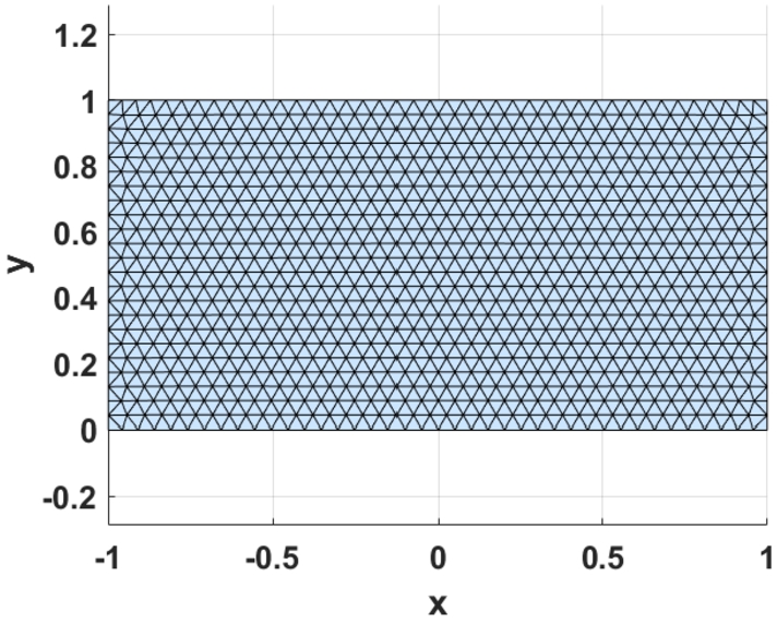
Test 1: For the first test, we consider a rectangular domain $\begin{matrix} Ω_{1} = {(x, y) / - 1 < x < 1 and 0 < y < 1} \end{matrix}$ with a triangulation discretization (see the mesh-grid in Fig. 1), which consists of 3766 nodes and 1819 elements, and take the following initial conditions: $\begin{matrix} u_{0} (x, y) = y^{2} {(1 - y)}^{2} {(1 - x^{2})}^{2}, v_{0} (x, y) = \frac{3}{2} y^{2} {(1 - y)}^{2} {(1 - x^{2})}^{2}, u_{1} = v_{1} = 0 . \end{matrix}$

Fig. 1.

Uniform mesh grid of $Ω_{1}$ .

Fig. 2.

Test 1: the numerical solution at different times.

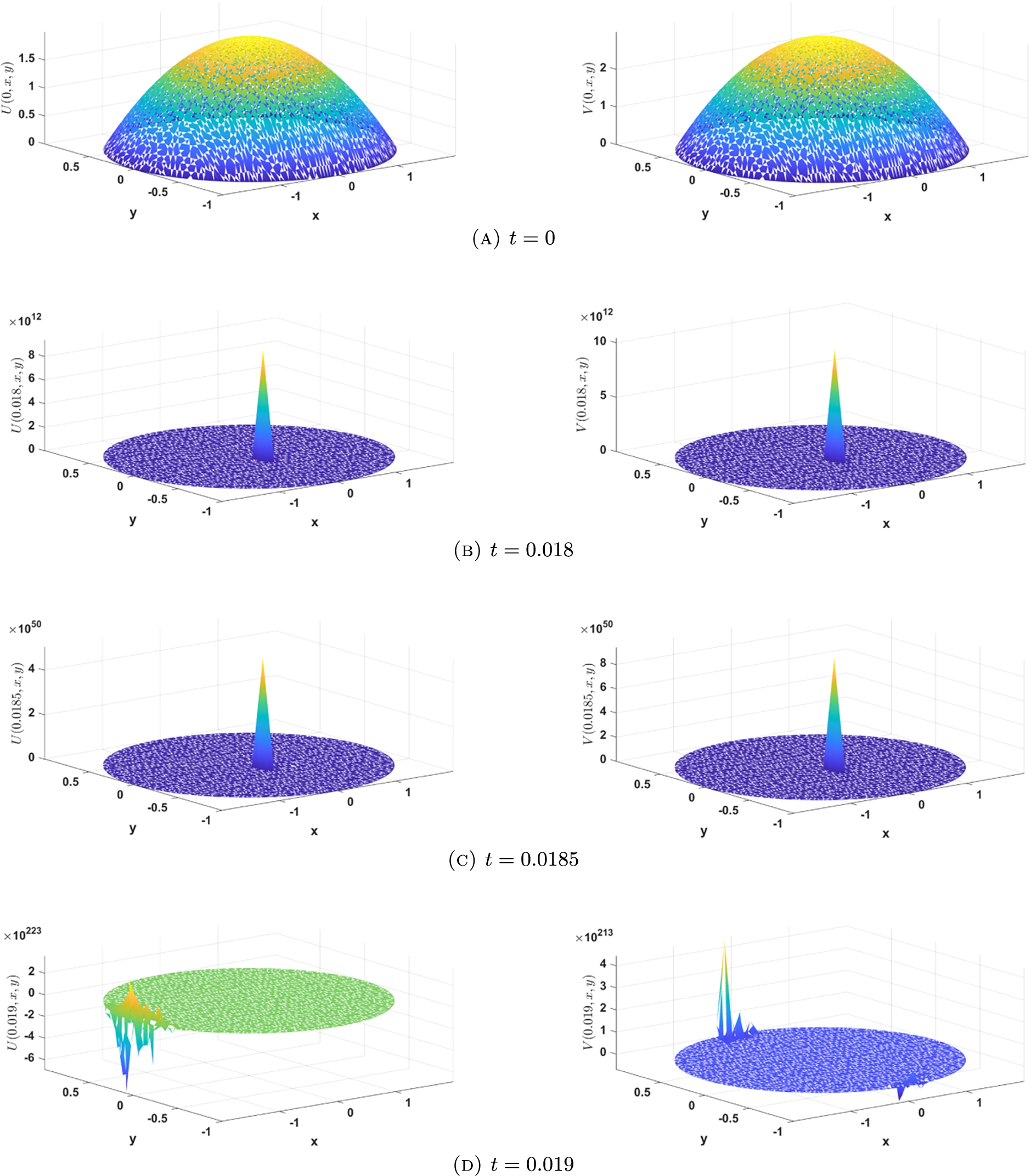
Figure 2 shows the approximate numerical results of the solution $(u, v)$ at different time iterations $t = 0$ , $t = 0.025$ , $t = 0.043$ and $t = 0.0445$ , where the left column shows the approximate values of u and the right column shows the approximate values of v.

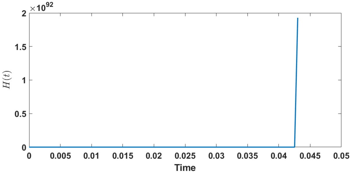
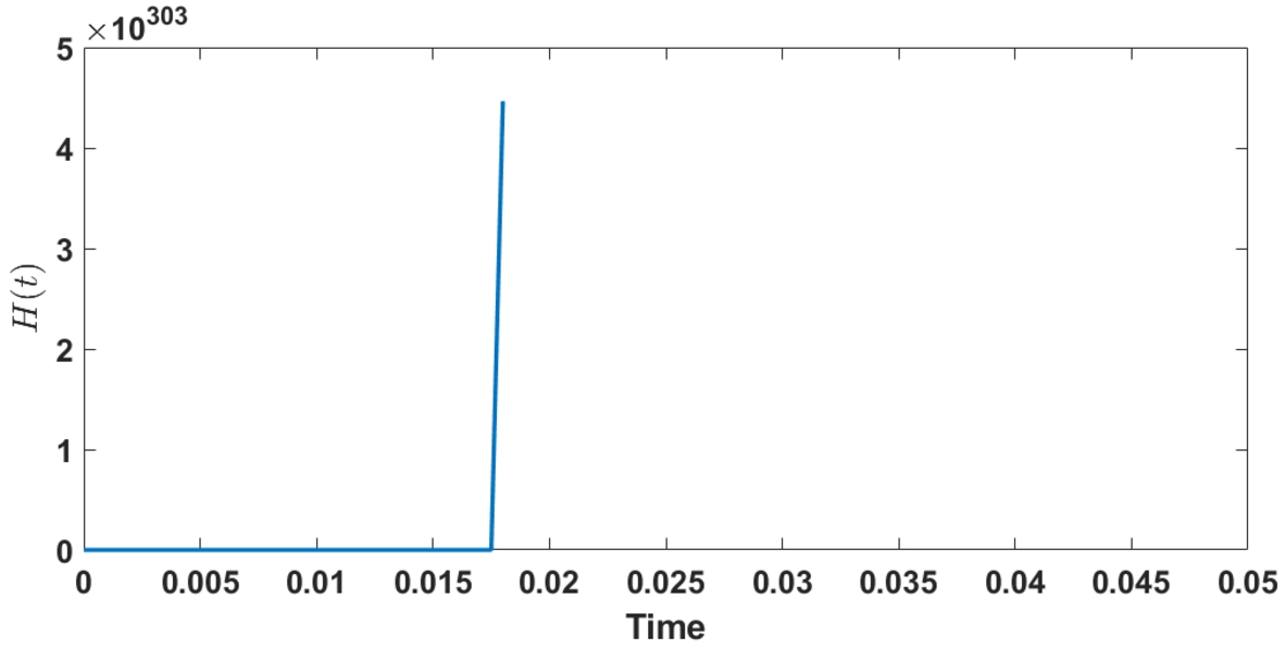
Figure 3 presents the numerical values of the functional $H (t)$ defined by (4.5) during the time iterations. It shows the blow-up of the energy of the system (1.1). Notice that the blow-up is occurring at instant $t = 0.0425$ .

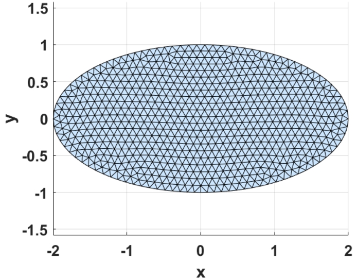
Test 2: For the second test, we consider an elliptical domain $\begin{matrix} Ω_{2} = {(x, y) / \frac{x^{2}}{4} + y^{2} < 1} \end{matrix}$ with a triangulation discretization (see the mesh-grid in Fig. 4), which consists of 2792 nodes and 1349 elements, and take the following initial conditions: $\begin{matrix} u_{0} (x, y) = 2 (1 - \frac{x^{2}}{4} - y^{2}), v_{0} (x, y) = 3 (1 - \frac{x^{2}}{4} - y^{2}), u_{1} = v_{1} = 0 . \end{matrix}$

Fig. 3.

Test 1: the blow-up of H in finite time.

Fig. 4.

Uniform mesh grid of $Ω_{2}$ .

Fig. 5.

Test 2: the numerical solution at different times.

For Test 2, Fig. 5 presents the approximate numerical results of the solution $(u, v)$ at different time iterations $t = 0$ , $t = 0.018$ , $t = 0.0185$ and $t = 0.019$ , where the left column shows the approximate values of u and the right column shows the approximate values of v. The numerical values of the functional $H (t)$ are presented in Fig. 6. We observe the blow-up of the energy from $t = 0.0175$ .

Fig. 6.

Test 2: the blow-up of H in finite time.

As a conclusion, the computational simulations show the blow-up of the solution of system (1.1) at finite time, which is compatible with the theoretical results.

Footnotes

Acknowledgement

The authors thank the University Batna 2, University of Sharjah and University of La Rochelle. The second author is supported by KFUPM, grant # INCB2205.

References

Aassila and

Guesmia, Energy decay for a damped nonlinear hyperbolic equation, Appl. Math Lett. 12 (1999), 49–52. doi:10.1016/S0893-9659(98)00171-2.

Agre and

Rammaha, Systems of nonlinear wave equations with damping and source terms, Differential Integral Equations. 19 (2006), 1235–1270.

Alves,

Cavalcanti,

Cavalcanty,

Rammaha and

Toundykov, On existence, uniform decay rates and blow up for solutions of systems of nonlinear wave equations with damping and source terms, Discrete and Continuous Dynamical Systems Series S 2(3) (2009), 583–608. doi:10.3934/dcdss.2009.2.583.

L.E.

Andersson,

Elfving and

G.H.

Golub, Solution of biharmonic equations with application to radar imaging, J. Comp. and Appl. Math. 94(2) (1998), 153–180. doi:10.1016/S0377-0427(98)00079-X.

Antontsev,

Ferreira and

Piskin, Existence and blow up of solutions for a strongly damped Petrovsky equation with variable-exponent nonlinearities, Electronic Journal of Differential Equations 2021 (2021), 1–18. doi:10.58997/ejde.2021.84.

Antontsev and

Shmarev, Blow-up of solutions to parabolic equations with nonstandard growth conditions, J. Comput. Appl. Math. 234(9) (2010), 2633–2645. doi:10.1016/j.cam.2010.01.026.

Antontsev and

Shmarev, Evolution PDEs with Nonstandard Growth Conditions, Atlantis Studies in Differential Equations, Vol. 4, Atlantis Press, Paris, 2015.

H.T.

Banks,

Ito and

Wang, Well-posedness for damped second order systems with unbounded input operators, Differential and Integral Equations. 8 (1995), 587–606.

M.I.G.

Bloor and

M.J.

Wilson, An approximate analytic solution method for the biharmonic problem, Proccedings of the Royal Society A: Mathiematical, Physical and Engineering Science. 462 (2006), 1107–1121.

10.

Bouhoufani and

Hamchi, Coupled system of nonlinear hyperbolic equations with variable-exponents: Global existence and Stability, Mediterranean Journal of Mathematics 17(166) (2020). doi:10.1007/s00009-020-01589-1.

11.

Bouhoufani,

S.A.

Messaoudi and

Zahri, Existence and decay of solutions for a coupled system of nonlinear wave equations with variable exponents, Elect. J. Differential Eqns. 73 (2023), 1–20.

12.

D.V.

Cruz-Urib and

Fiorenza, Variable Lebesgue Space: Foundations and Harmonic Analysis, Springer, Heidelberg New York Dordrecht London, 2013.

13.

Georgiev and

Todorova, Existence of solutions of the wave equation with nonlinear damping and source terms, J. Diff. Eqns. 109 (1994), 295–308. doi:10.1006/jdeq.1994.1051.

14.

Ghegal,

Hamchi and

S.A.

Messaoudi, Global existence and stability of a nonlinear wave equation with variable-exponent nonlinearities, Applicable Analysis. 99(8) (2020), 1333–1343. doi:10.1080/00036811.2018.1530760.

15.

Guesmia, Existence globale et stabilisation interne non linéaire d’un systeme de Petrovisky, Bell. Belg. Math. Soc. 5 (1998), 583–594.

16.

Guesmia, Energy decay for a damped nonlinear coupled system, J. Math. Anal. Appl. 239 (1999), 38–48. doi:10.1006/jmaa.1999.6534.

17.

Guo and

Gao, Blow up of solutions to quasilinear hyperbolic equations with

p (x, t)

-Laplacian and positive initial energy, C. R. Mecanique. 342 (2014), 513–519. doi:10.1016/j.crme.2014.06.001.

18.

J.H.

Hassan, General decay results for a viscoelastic wave equation with a variable exponent nonlinearity, in: Asymptotic Analysis., Vol. 125, IOS Press, 2021, pp. 365–388. doi:10.3233/ASY-201661.

19.

Komornik, Exact Controllability and Stabilization. the Multiplier Method, Masson, Paris, 1994.

20.

Komornik, Well-posedness and decay estimates for a Petrovesky system by a semigroup approach, Acta. Sci. Math. (Szeged) 60 (1995), 451–466.

21.

Lars,

Hasto and

Ruzicka, Lebesgue and Sobolev Spaces with Variable Exponents, Lect Notes Math, Springer, 2011.

22.

A.C.

Lazer and

P.J.

Mckenna, Large-amplitude periodique oscillations in suspension bridges: Some new connections with nonlinear analysis, Siam Review. 32(4) (1990), 537–578. doi:10.1137/1032120.

23.

Li,

Guo and

Liao, Asymptotic stabilty of solutions to quasilinear hyperbolic equations with variable sources, Computers and Mathematics with Applications. 79(4) (2000), 1012–1022. doi:10.1016/J.camwa.2019.08.016.

24.

Liao and

Tan, On behavior of solutions to a Petrovsky equation with damping and variable-exponent source, Math. App. (2021), 1–21.

25.

J.L.

Lions, Quelques Méthodes de Résolution des Problemes aux Limites Nonlinéaires, 2nd edn, Dunod, Paris, 2002.

26.

Messaoudi,

Bouhoufani,

Hamchi and

Alahyane, Existence and blow up in a system of wave equations with nonstandard nonlinearities, Electronic Journal of Differential Equations. 91 (2021), 1–33.

27.

Messaoudi and

Talahmeh, Blow up in solutions of a quasilinear wave equation with variable-exponent nonlinearities, Mathematical Methods in the Applied Sciences 40(18) (2017), 6976–6986. doi:10.1002/mma.4505.

28.

Messaoudi and

Talahmeh, Blow up of negative initial-energy solutions of a system of nonlinear wave equations with variable-exponent nonlinearities, Discrete and Continuous Dynamical Systems Series S, to appear.

29.

Messaoudi,

Talahmeh and

Al-Gharabli, On the existence and stability of a nonlinear wave system with variable exponents, in: Asymptotic Analysis., Vol. 1, IOS Press, 2021, pp. 1–28. doi:10.3233/ASY-211704.

30.

Messaoudi,

Talahmeh and

Al-Smail, Nonlinear damped wave equation: Existence and blow-up, Computers and Mathematics with applications. 74(12) (2017), 3024–3041. doi:10.1016/j.camwa.2017.07.048.

31.

S.A.

Messaoudi, Global existence and nonexistence in a system of Petrovsky, Journal of Mathematical Analysis and Applications. 265 (2002), 296–308. doi:10.1006/jmaa.2001.7697.

32.

S.A.

Messaoudi,

J.H.

Al-Smail and

A.A.

Talahmeh, Decay for solutions of a nonlinear damped wave equation with variable-exponent nonlinearities, Computers and Mathematics with applications. 76(8) (2018), 1863–1875. doi:10.1016/j.camwa.2018.07.035.

33.

S.-H.

Park and

J.-R.

Kang, Blow-up of solutions for a viscoelastic wave equation with variable exponents, Math. Meth. Appl. Sci. 42 (2019), 2083–2097. doi:10.1002/mma.5501.

34.

J.A.

Pelesko and

D.H.

Bernstein, Modeling Mems and Nems, CRC Press, 2002.

35.

Ružička, Electrorheological Fluids: Modeling and Mathematical Theory, Lecture Notes in Mathematics, Vol. 1748, Springer, Berling, Heidelberg, 2000.

36.

T.V.

Smitha,

K.V.

Nagaraja and

Sarada, Matlab 2D higher-order triangle mesh generator with finite element applications using subparametric transformations, Advances in Engineering Software 115 (2018), 327–356. doi:10.1016/j.advengsoft.2017.10.012.

37.

Timoshenko and

W.K.

Sergius, Theory of Plates and Shells, 2nd edn, McGraw-Hill, New York, 1995, 138317481406.

38.

Xiaolei,

Bin and

Menglan, Asymptotic stability of solutions to quasilinear hyperbolic equations with variable sources, Computers and Mathematics with Applications (2019), 1–11.