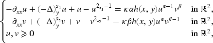
This article focuses on the existence and non-existence of solutions for the following system of local and nonlocal type
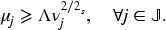
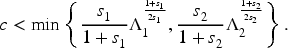
where , , , and , . The existence of a ground state solution entirely depends on the behaviour of the parameter and on the function h. In this article, we prove that a ground state solution exists in the subcritical case if κ is large enough and h satisfies (H). Further, if κ becomes very small, then there is no solution to our system. The study of the critical case, i.e., , , is more complex, and the solution exists only for large κ and radial h satisfying (H1). Finally, we establish a Pohozaev identity which enables us to prove the non-existence results under some smooth assumptions on h.
In this article, we study the existence and non-existence of solutions for the following system associated with mixed Schrödinger operator:
where . The exponent , is known as a critical exponent and it plays a vital role in the existence and non-existence of solutions to the system (1.1). The parameter and α, β are chosen such that
Throughout this paper we always assume that the function h satisfies the following condition
To study the motivation and the applications of the mixed Schrödinger operator in detail, we refer to the article [5] and the references therein. In 2018, Amin Esfahani et al. [5] dealt with the following problem
where and the operator denotes the fractional Laplacian with respect to x-variable, which is defined (on appropriate functions) in Cauchy principle value (p.v.) sense up to a normalizing constant by
The function satisfies the subcritical growth assumptions without Ambrosetti–Rabinowitz type condition. The equation (1.2) admits a positive radial ground state solution (see [5, Theorem 1.3]). In 2019, Felmer and Wang [6] also considered the problem of type (1.2) and studied the qualitative properties of positive solutions under different assumptions on f. Recently, Gou et al. [7] provided a comprehensive study about the existence and non-existence of solutions to the following problem on a plane
The authors proved that the problem (1.3) has a positive ground state solution which is axially symmetric for , and using Pohozaev identity it has only trivial solution for . If , the system (1.1) reduces to a single equation of the form
which clearly does not possess any non-trivial solution by taking in (1.3). This shows that the system (1.1) has no semi-trivial solutions, i.e. solutions like or . In this article, we are interested in the effects of κ and on the existence of fully non-trivial solutions (particularly, ground state solutions, whose definition will be given later) for the system (1.1), i.e. solutions with and . Since the equation (1.3) has non-trivial solutions for (see [7]), when , we expect that a large κ and positive h will bring the existence of ground state solutions for (1.1). Indeed, as readers will see, our expection is right. Further, this is right when . Situations become more complex in the critical case that , . On the one hand, we can prove that a solution exists under a setting that κ is large and h is radial and satisfies the following assumption (H1):
On the other hand, the system (1.1) has no non-trivial solutions for some h, such as h being a positive constant, and more examples of h will be given later. Our study opens a door to understand that the conditions on κ and h are crucial for the existence and non-existence of non-trivial solution for (1.1).
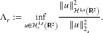
To state our main results, we first define the fractional Sobolev–Liouville space (see [4]). The space is a Banach space with respect to the norm
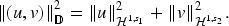
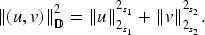
The product space is endowed with the norm
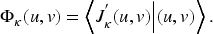
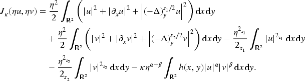
The energy functional associated with the system (1.1) is defined by and given as follows:
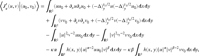
The above functional is well-defined and on the product space . For , the Fréchet derivative of at is represented as
where is the Fréchet derivative of at , and the duality bracket between the product space and its dual is represented as . We just write if no confusion of notation arises.
(Ground state solution)
A non-trivial critical point of over is said to be a ground state solution if its energy is minimal among all the non-trivial critical points i.e.
As explained in Section 2 below, the functional is not bounded from below on the product space . For this reason, we introduce the definition of Nehari manifold associated with the functional as
where
Define . Notice that the Nehari manifold consists of all non-trivial critical points of . Hence, if can be achieved by some , then is a ground state solution.
We have the following conclusions:
is non-increasing w.r.t., and further,for allifcan be achieved;
is continuous w.r.t.;
there existssuch that
wherewill be defined by (3.3).
It is open whether or not.
We are firstly concerned with the case that or .
Letor. Recall thatis given by Proposition 2. Then we have:
for any,has a minimizer, which is a non-negative (constant sign) ground state solution to the system (1.1);
for any,has no minimizers.
Next we focus on the critical case that , , which is more complex.
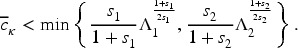
Suppose,and that h is radial satisfying (H1). Then there is(which will be given by Proposition 7 ) such that for any, there exists a non-negative (constant sign) non-trivial solution to the system ( 1.1).
It is still open whether the solution exists or not in the critical case for small enough.
To prove Theorem 5, we find solutions in the radial space where
We further define
where
Let , and
Similar to Proposition 2, we have the following result.
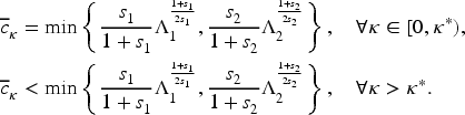
Under the assumptions of Theorem 5, we have the following conclusions:
is non-increasing w.r.t., and further,for allifcan be achieved;
is continuous w.r.t.;
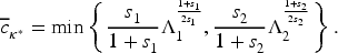
there existssuch that
On the other hand, for some h, (1.1) has no non-trivial solutions.
(Non-existence of non-trivial solutions)
Let,. If h and κ satisfy either of the following hypothesis:
h is a positive constant and κ is any real number,
such thatand,
then the system (1.1) has no non-trivial solutionwhich satisfies.
We organize the rest of our paper as follows. The Section 2 contains some properties of the Nehari manifold and the boundedness of (PS) sequences. Further, the fractional Laplacian w.r.t y variable is defined and some useful results associated with it are demonstrated. In Section 3, the concentration-compactness tools for the mixed Schrödinger operator are developed and using this tool we prove the (PS) compactness condition of in the subcritical case. In Section 4, some properties of and the proof of Theorem 4 are given. In Section 5, we give the proof of Theorem 5. Finally, we establish the Pohozaev identity in Section 6 and using this Pohozaev identity we give the non-existence result (see Theorem 8). We conclude this section by providing some specific examples of h for which the non-trivial solution does not exist.
Observe that the functional as η becomes very large. Since is not bounded from below on , we try to minimize the given functional on the Nehari manifold in order to find a critical point in via variational approach.
If we consider , then the following identity holds
The restriction of on is given as
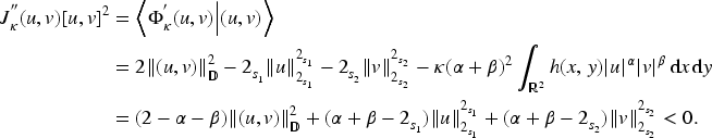
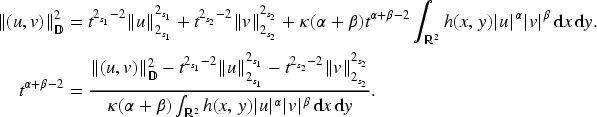
Further, if for all , using the identity (2.2) we obtain an algebraic equation of the form
By following a careful analysis on the above algebraic equation, it has a unique positive solution. Hence, there exists a unique such that for all . For any , the identity (2.2) and the assumption (${\alpha \beta}$) altogether yield
From above, we deduce the following
Moreover, by the identity (2.2) there exists a such that the product norm is bounded from below i.e.,
Using the Lagrange multiplier method, if is a critical point of on the Nehari manifold , then there exists a called Lagrange multiplier such that
Further calculations yields . It is clear that , otherwise the inequality (2.5) does not hold and subsequently we obtain . Hence, there is a one-to-one correspondence between the critical points of and the critical points of . The functional restricted on can also be written as
Now the hypotheses (${\alpha \beta}$) and (2.7) combined with (2.8) give the following inequality
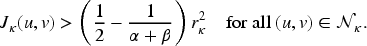
Notice that restricted on is bounded from below. Hence, we can expect the solution of (1.1) by minimizing the energy functional on the Nehari manifold . Further, such a minimizer on is a ground state solution since consists of all non-trivial critical points of .
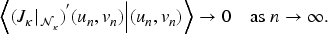
Next we prove that the (PS) sequences on are bounded in .
If is a (PS) sequence for on at level under the hypotheses (${\alpha \beta}$) and (H), then is a bounded (PS) sequence for in .
Given is a (PS) sequence for at level c, then by definition
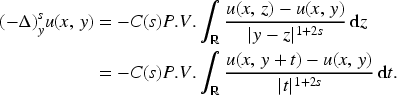
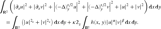
We denote as the classical Laplacian operator w.r.t y variable and its fractional analogue i.e., the fractional Laplacian operator w.r.t y variable denoted by is defined on smooth functions as
where is a normalizing constant and the abbreviation P.V. means the principal value sense. Since we are dealing our problem (1.1) in , we choose and . So the formal definition takes the following form
where
Due to the singularity of the kernal, the right-hand side of (2.15) is not well defined in general. In fact for the integral in (2.15) is not really singular near y. In the following, we prove the analogous results of Hitchiker’s guide [3].
Letand letbe the fractional Laplacian operator defined by (2.15). Then, for any(Schwartz space of rapidly decaying functions),
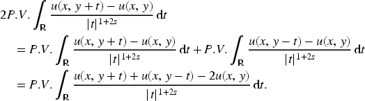
By choosing , we have
Now by substituting in last term of the above equality, we have
So after relabeling as t
Therefore, if we replace t by z in (2.18) and (2.20), we can write the fractional Laplacian operator in (2.15) as
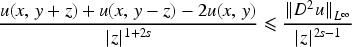
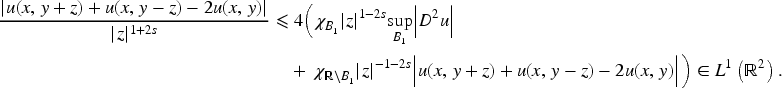
The above representation is useful to remove the singularity at the origin. Indeed, for any smooth function u, a second order Taylor expansion yields,
which is integrable near 0 (for any fixed ). Therefore, since , one can get rid of the . and write (2.17).
One can observe that the operator is indeed well-defined for any . If we take any non-zero constant, it does not belong to the Schwartz space but it is fractional harmonic.
For any , the Fourier transform of u is well-defined and it is given by
For, letbe the fractional Laplacian operator given by (2.15). Then, for any,
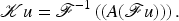
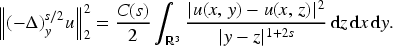
The Lemma 11 represents the fractional Laplacian w.r.t. y variable as a second order differential quotient given by (2.17). We denote by the integral in (2.17), i.e.
is a linear operator and our goal is to look for a function such that
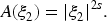
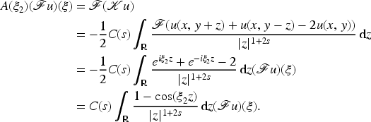
Indeed, we seek for A satisfying
Further, we have the following estimate
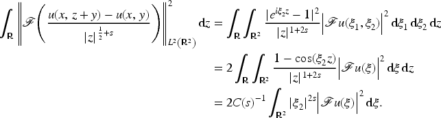
Hence, by the Fubini–Tonelli theorem we can exchange the integral in z with the Fourier transform in . Applying Fourier transform we obtain
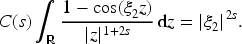
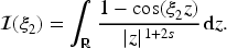
Notice that the above Proposition is important in the sense that it gives us an equivalence relation between the Fourier norm and the Gagliardo semi-norm. Since our problem is of variational type, it is natural to work with the Gagliardo semi-norm than Fourier norm. Moreover, we also write (see [5, Remark 1.1])
We define the fractional gradient w.r.t y variable for as
The next two lemmas are due to [1, Lemma 2.2, Lemma 2.4]. The proof follows by similar arguments and therefore we omit the details.
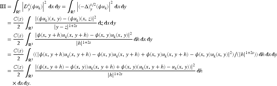
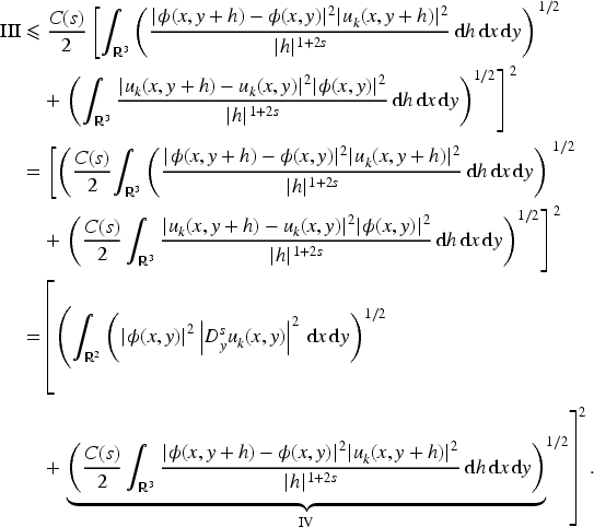
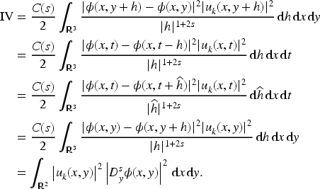
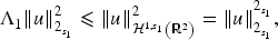
Letbe such that. Then, there exists a constantdepending on s andsuch that
Letandbe such that there existandsuch that
If, then, whereis the weighted-space with weight w and the symbol “” means the compact embedding.
If has compact support, then verifies all the assumptions of the above lemma.
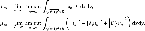
.Concentration–compactness
In this section, we recall the following result by Lions [8, Lemma 1.2], which we will be using further to prove the concentration-compactness results.
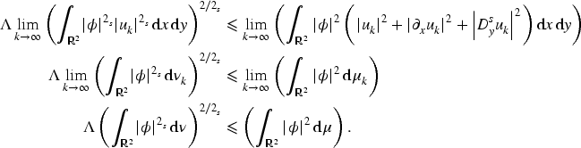
Let ν, μ be two non-negative, bounded measures onsuch that
for some constantand. Then there exist a countable setandsuch that
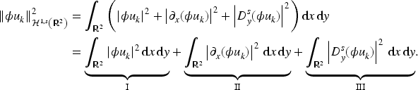
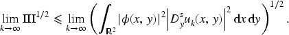
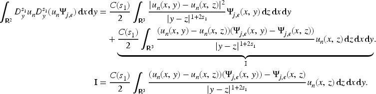
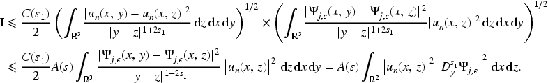
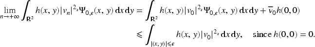
Using Remark 18, the weight verifies all the hypothesis of Lemma 17. Therefore, the sequence converges strongly to in . Hence, we obtain
Further,
and
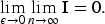
The second term in the last inequality tends to 0 as using a similar set of arguments as in Lemma 17. Subsequently, we have
Thus we have
Further,
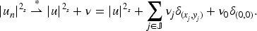
Now by Lemma 19, there exists a countable set , points and positive weights such that
where and are Dirac measures centred at points and respectively.
Now if , we replace by . Since weakly in , the sequence in . Let (the set of all continuous bounded functions), then Brezis–Lieb Lemma 20 yields
Consequently we obtain
Applying the Brezis–Lieb lemma again, we obtain
which further gives
Moreover, we also have
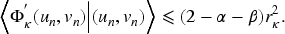
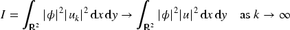
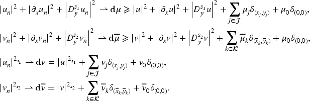
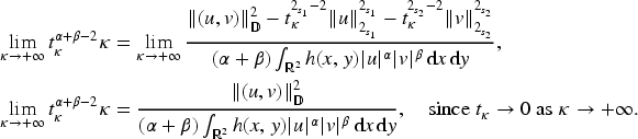
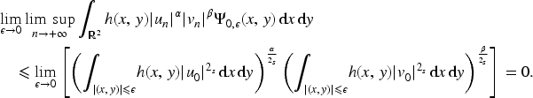
Suppose or and h satisfies (H). Then the functional satisfies the (PS)-condition at level c satisfying
Let be a (PS)-sequence for in . Then is a bounded sequence in (see Lemma 10) and by reflexivity there exists a subsequence still denoted by itself and satisfying the following
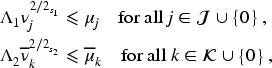
Now using (3.13), (3.14) and (3.15), which are analogous to the concentration–compactness principle of Bonder [1, Theorem 1.1], there exist a subsequence, still denoted as , two at most countable sets of points and , and non-negative numbers
such that the following convergences hold weakly∗ in the sense of measures,
Moreover,
where , , are the Dirac measures at the points , of respectively. We denote the concentration of the sequence at infinity by the following numbers
We similarly define the concentrations of the sequence at infinity by the numbers and . Now let us take a smooth cut-off function centered at and defined as
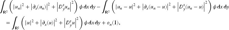
where . Testing with we have
Now
Since is a bounded sequence in , the Hölder’s inequality gives
If the concentration is considered at the point only, i.e. and further from (3.30) we see that
From (3.16) we conclude that for all . Arguing similarly we also have for all . Now if , then
which contradicts the assumption (3.16). Therefore, . By the same token, we also get . Arguing in a similar way we also get . Hence, there exists a subsequence that strongly converges in . Furthermore, we have
which infers that the sequence strongly converges in and the (PS) condition holds.
.Properties of and proof of Theorem 4
We are devoted to prove Proposition 2 in the first part of this section.
Proof to Proposition 2.
Firstly, we prove (1). Let . We take a bounded (in ) minimizing sequence converging to . There exists a unique such that . Thus, we have
where we use (2.6) in the first inequality. Sending n to infinity, one gets . Furthermore, if is achieved by , we know and . There exists a unique such that . Then we have
This completes the proof to (1).
Next, we prove (2). By (1), it is sufficient to prove that for all . For any sequence with , we can take a bounded (in ) sequence such that . There exists a unique such that . We claim that is bounded. Indeed, if up to subsequences, using (2.4) (for ) we have , , as . Then using (2.4) again (for ) one gets , which is a contradiction. Hence, is bounded. Then we have
Sending n to infinity, one gets . The proof to (2) is complete.
Finally, we prove (3). We firstly prove that . (2.2) reads in the case that for any ,
We will consider three cases: , ; , ; and , . When , , from
Then we can deduce that . On the other hand, WLOG, we assume that . Take a minimizing sequence to , i.e., as . By replacing by (also denoted by ) for some , we may assume that . Then
implying that . Hence, we obtain that .
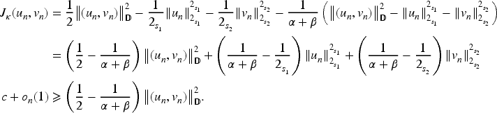
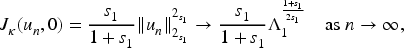
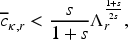
Further, We prove that for κ large enough. For any , there exists a unique such that and satisfies the algebraic equation
Suppose , then using the assumption we get . Subsequently, we can write
Further we check the behaviour of the functional as . The functional is given by
The term is given by
Notice that as . Hence, as and there exists a such that if , where is sufficiently large, then . Thus we obtain
and hence from the above inequality we get
Now we know that there exists such that
Since is continuous, we have
The proof is complete.
In the rest part of this section, we prove Theorem 4.
Proof of Theorem 4.
We firstly consider the case that and prove (1). By Proposition 2-(3),
for any . Then we use Lemma 22 to ensure the existence of such that . Next, we define the function given by , for all . Then
where , , , . Clearly, , , are non-negative. The condition implies that , . Therefore the function is strictly concave for . Also, we have and . Moreover, the function for small enough. Hence, has a unique global maximum point at and has a unique root at and for , in particular . Also, from the equation (2.5) and , we observe that if and only if .
Now we consider the function , then from the above arguments there exists a unique such that and satisfies the following algebraic equation
Moreover, the pair gives
Now from the inequality , one finds that . Since and is the unique maximum point of , . We can deduce that
Thus, we can assume that and in . If , then satisfies the equation
which implies , since the above equation has only trivial solution (see [7, Lemma 2.2]). Therefore, we get a contradiction to the fact that . So we can conclude that either or is not identically zero.
Notice that the Nehari manifold consists of all the non-trivial critical points of the functional . This implies that . On the other hand, . Hence, , and so is a non-negative (constant sign) ground state solution to the system (1.1).
Next, we consider the case that and prove (2). Suppose on the contrary that there exists a such that has a minimizer. By Proposition 2-(1), we have , which is a contradiction to Proposition 2-(3). The proof is complete.
Notice that we have derived only the non-negative solutions and to obtain a positive solution we require the maximum principle for the mixed type Schrödinger operator.
.Proofs of Theorem 5
The proof of Proposition 7 is similar to the one of Proposition 2 and we omit the details.
To prove Theorem 5, we firstly give a preliminary compactness result in the critical case. Recall that (H1) is given as
and the space of radial functions in is defined as
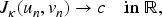
If and h is a radial function satisfying (H1). If is a (PS) sequence for at level such that c satisfies
the sequenceadmits a strongly converging subsequence in.
Since the functions are radial, having concentrations at points other than gives a contradiction to countability of concentration points. Now if we want to avoid concentration at the points 0 and ∞, it is sufficient to show that
where the cut-off function is centred at satisfying (3.20) and the cut-off function supported near ∞ satisfying the following for large enough
For any , the assumption implies that . Using the assumption on h in (H1) and the Hölder’s inequality, we get
From the above three inequalities, it follows that
Similarly, we can prove (5.3) using the assumption that .
Then using similar arguments to Lemma 22, we can complete the proof.
Proof of Theorem 5.
By Proposition 7-(3),
for any . We use Lemma 24 to ensure the existence of such that . Then similar to the proof of Theorem 4, we know is a non-negative (constant sign) non-trivial solution to the system (1.1). The proof is complete.
.Proof of Theorem 8
In the following we prove the Pohozaev type identity which will be useful to derive the non-existence results to the system (1.1).
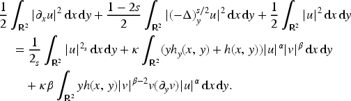
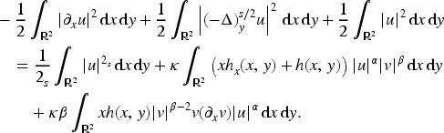
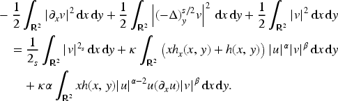
Assume thatis a solution to (1.1) such that,, and. Thensatisfies the following necessary conditions:
and
Let denotes the Fourier transform of u defined by
and denotes the inverse Fourier transform of u. Then we observe that
Now we are going to prove the non-existence result using the previous lemma.
Proof of Theorem 8.
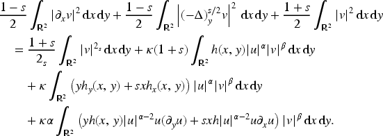
Let be a solution to (1.1) such that . We first divide the equation (6.1) by s and subsequently, we subtract (6.1) into (6.2) to get
One can notice that for i.e., there is only a trivial solution for . Moreover, if h is a constant function and κ is any real number, from (6.22) we have
which implies u, v are both identically zero a.e. Hence, there does not exist any non-trivial solution to (1.1) for this case.
We are given that satisfies , . Using the hypotheses on h in (6.22), we deduce that
From above inequality, we can conclude that u, v are both identically zero almost everywhere. Hence, there does not exist any non-trivial solution to (1.1) for such h.
The following examples of h ensure the non-existence of solutions to (1.1).
If we consider
then and , for . Thus by Theorem (8), there does not exist any non-trivial solution to (1.1) such that .
Moreover, if , then with and for . As a result, no non-trivial solution exists to (1.1) such that .
Footnotes
Acknowledgements
RK acknowledges the support of the CSIR fellowship, file no. 09/1125(0016)/2020–EMR–I. TM acknowledges the support of the Start up Research Grant from DST-SERB, sanction no. SRG/2022/000524.
References
1.
BonderJ.F.SaintierN.SilvaA., The concentration-compactness principle for fractional order Sobolev spaces in unbounded domains and applications to the generalized fractional Brézis-Nirenberg problem, NoDEA Nonlinear Differential Equations Appl.25(6) (2018), 52, 25.
2.
BrézisH.LiebE., A relation between pointwise convergence of functions and convergence of functionals, Proceedings of the American Mathematical Society88(3) (1983), 486–490. doi:10.1090/S0002-9939-1983-0699419-3.
3.
Di NezzaE.PalatucciG.ValdinociE., Hitchhiker’s guide to the fractional Sobolev spaces, Bull. Sci. Math.136(5) (2012), 521–573. doi:10.1016/j.bulsci.2011.12.004.
4.
EsfahaniA., Anisotropic Gagliardo–Nirenberg inequality with fractional derivatives, Z. Angew. Math. Phys.66(6) (2015), 3345–3356. doi:10.1007/s00033-015-0586-y.
5.
EsfahaniA.Ehsan EsfahaniS., Positive and nodal solutions of the generalized BO–ZK equation, Rev. R. Acad. Cienc. Exactas Fís. Nat. Ser. A Mat. RACSAM112(4) (2018), 1381–1390. doi:10.1007/s13398-017-0435-2.
6.
FelmerP.WangY., Qualitative properties of positive solutions for mixed integro-differential equations, Discrete Contin. Dyn. Syst.39(1) (2019), 369–393. doi:10.3934/dcds.2019015.
7.
GouT.HajaiejH.StefanovA.G., On the solitary waves for anisotropic nonlinear Schrödinger models on the plane, Eur. J. Math.9(3) (2023), 55, 34.
8.
LionsP.-L., The concentration-compactness principle in the calculus of variations. The limit case. I & II, Rev. Mat. Iberoamericana1(1) (1985), 45–121, 145–201. doi:10.4171/rmi/6.
9.
XiangM.ZhangB.ZhangX., A nonhomogeneous fractional p-Kirchhoff type problem involving critical exponent in , Adv. Nonlinear Stud.17(3) (2017), 611–640. doi:10.1515/ans-2016-6002.