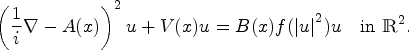
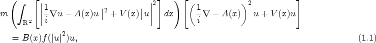
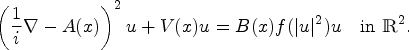
In this paper, we are concerned with the following magnetic nonlinear equation of Kirchhoff type with critical exponential growth and an indefinite potential in
where , m is a Kirchhoff type function, and represent locally bounded potentials, while B denotes locally bounded and f exhibits critical exponential growth. By employing variational methods and utilizing the modified Trudinger–Moser inequality, we get ground state solutions or nontrivial solutions for the above equation. Furthermore, in the special case where m is a constant equal to 1, the equation is reduced to the following magnetic nonlinear Schrödinger equation,
Applying analogous methods, we can also establish the existence of ground state solutions or nontrivial solutions to this equation.
In this paper, we study the following nonlinear Kirchhoff–Schrödinger equation in
where and the nonlinearity are the continuous functions, , , and the magnetic potential . The potential V may be non-positive on some subset with positive measure and f has critical exponential growth.
Generally speaking, the presence of the term
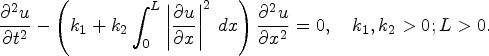
which depends on the gradient of u with respect to the magnetic field, renders the equation nonlocal and distinguishes it from pointwise identities. This nonlocal character makes the study of equation (1.1) particularly difficult and interesting. Firstly, Kirchhoff [25] conducted pioneering research on the lateral vibrations of elastic strings, culminating in the formulation of a hyperbolic equation that describes this dynamic behavior. The equation takes the form:
This equation accounts for the nonuniform distribution of vibrational energy along the string, introducing the integral term to capture the string’s dynamic response. For further insight into the early developments of Kirchhoff equations, readers are encouraged to explore the works cited in [11,22,24,31]. Additionally, there are many papers on the nonlocal Kirchhoff problems, see [3,14] and the references therein.
In particular, for the case that , if is replaced by , Li and Yang [26] studied the following N-Kirchhoff problem
where for , , is the N-Laplacian operator of u, λ is a real positive parameter, , with and with critical exponential growth. By establishing suitable assumptions on the functions V and f, they demonstrated the existence of a positive constant Λ such that problem (1.2) admits at least two positive solutions for any .
Generally, for the case of , Xiang, Pucci, Squassina and Zhang [36] dealt with the existence and multiplicity of solutions to the following Kirchhoff–Schrödinger equation involving an external magnetic potential
where , , , , is a magnetic potential, is the fractional magnetic operator and denotes an electric potential.
Within our research framework in , a considerable body of literature has explored the existence and multiplicity of bound state solutions for equations similar to (1.1). When , Furtado and Zanata [23] investigated the following analogous nonlinear Kirchhoff equation
where , , the Kirchhoff function is a continuous function and the nonlinearity is a continuous function with critical exponential growth. By establishing certain assumptions on the functions m, b, B and f, they demonstrated that the equation (1.3) possesses at least one nonnegative ground state solution or a nonnegative nontrivial solution. In the special case where of , equation (1.3) reduces to the following nonlinear Schrödinger equation
for which they also obtained similar results.
In addition, for the case of , when , equation (1.1) simplifies to the following magnetic Schrödinger equation
which means that our problem has become a local situation. Equation (1.4) appears when seeking the standing wave solutions , with , of the planar Schrödinger equation
And the operator
appears when the interaction between the material field ψ and the external electromagnetic field with potential U and magnetic potential A is studied through the minimum coupling rule. Additionally, d’Avenia and Ji [17,18] investigated the following magnetic nonlinear Schrödinger equation similar to (1.4)
where is a parameter, and are continuous potentials and the nonlinearity exhibits critical growth. Under certain assumptions on the potential V, they employed variational methods and Ljusternick–Schnirelmann theory to prove the existence of a multiplicity of solutions and their concentration for small in (1.5).
In summary, the magnetic nonlinear Schrödinger equations have been the subject of extensive research by numerous authors, who have employed a variety of appropriate methods to study them. See [4,7–9,15,16,21,27,35] and the references therein for a comprehensive overview. In particular, Ambrosio and d’Avenia [6] focused on the following magnetic nonlinear fractional Schrödinger equation
where is a positive parameter, , denotes the fractional magnetic Laplacian, , and are continuous potential and is a subcritical nonlinearity. Using variational methods and Ljusternick–Schnirelmann theory, they proved that the existence and multiplicity of solutions to (1.6) for small. Ambrosio [5] explored a fractional magnetic Schrödinger equation with exponential critical growth in and established a multiplicity result. Additionally, an existing result of a magnetic Schrödinger equation with periodic magnetic potential satisfying a local integrability condition was studied by Bégout [10]. However, due to the presence of the magnetic potential A and the nonlocal term, our equation (1.1) becomes a complex-valued problem, and the weak limit of the energy functional’s () sequence may not correspond to a solution of the original problem, which means that more dedicated estimates are needed. Furthermore, relatively few papers have investigated magnetic nonlinear nonlocal equations with critical exponential growth, a topic that greatly interests us and motivates our current research.
Drawing upon the work in [18], we offer some insightful comments and discuss the functional space that will be employed in our study. For , we define
and
where
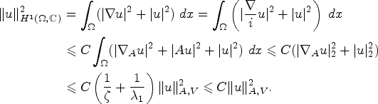
Clearly, is a subspace of and due to [28], we know that is a Hilbert space with the inner product and norm
Here, Re denotes the real part of a complex number, and the bar represents complex conjugation. Owing to the fact that , we can invoke [28, Theorem 7.21] to assert the diamagnetic inequality
for each . This inequality is a crucial tool in our subsequent analysis.
Focusing on potential V, we have the following notations
and for any open domain ,
where and is the closure of in .
Next, we give some assumptions about equation (1.1). The assumptions on the potential are:
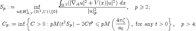
;
;
there exists such that
The assumptions on the potential are:
for any ;
there exist , and such that
where .
Assumptions ()–() and ()–() were originally introduced by Sirakov [33] in the context of subcritical Schrödinger equations in with . We will utilize these assumptions to ensure that is a Hilbert space and to derive some useful Sobolev embedding for our subsequent analysis below.
Now, let’s consider the nonlocal term and its associated assumptions:
;
for every , we have
where , ;
is decreasing in .
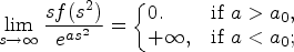
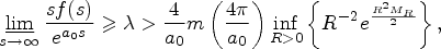
Next, we give two notations (with more details provided in Lemma 2.5 and the definition of ζ in Lemma 2.1) and the assumptions that the nonlinearity f satisfies
if ;
there exists such that
there exists such that
where , ;
is non-decreasing in ;
there exist such that
there exists such that
there exists such that
where
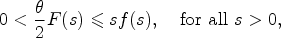
Conditions () and () guarantee that the solutions obtained from Theorems 1.1 and 1.2 are ground states. Nevertheless, as we will demonstrate in the proofs if we replace () and () with the weaker conditions () and the monotonicity result from Lemma 2.10 in the subsequent chapter, we can still obtain nontrivial solutions to problem (1.1) that are not necessarily ground states. The condition () is as follows:
for any , we can obtain that there exists such that
In virtue of (), we know that is non-decreasing and positive for . Consequently, for any , there exists such that
and
The main results of this paper are as follows.
Under assumptions ()–(), ()–(), ()–(), ()–(), problem (1.1) possesses a ground state solution.
Under assumptions ()–(), ()–(), (), ()–(), ()–() and (), problem (1.1) has a ground state solution, where condition () will be introduced in Section2.
Before starting the main results for the local case, we introduce a notation
It is evident that is finite and . In the local case, we can obtain similar results by adapting the approach used for nonlocal problems. Instead of conditions (), (), () and (), we consider the following assumptions:
there exists such that
where , ;
is non-decreasing in ;
there exists such that
there exists such that
Clearly, condition () is weaker than () and condition () is weaker than (). Our main results about (1.4) are the following.
Under assumptions ()–(), ()–() and ()–(), () and (), problem (1.4) has a nontrivial solution. In addition, if f satisfies (), the solution is a ground state.
Under assumptions ()–(), (), ()–(), ()–(), () and (), problem (1.4) has a nontrivial solution. In addition, if f satisfies (), the solution is a ground state.
This paper is organized as follows. We present several notations and technical lemmas in Section 2. In Section 3, we show the variational framework of problem (1.1). Minimax estimates are given in Section 4. In Section 5, we prove Theorems 1.1–1.2. Finally, in the last section, we prove Theorems 1.3–1.4.
Preliminaries
Hereafter, we use , , and to denote the norm of the space , , and , respectively. denotes the open ball centered at with radius and denotes the complement of in . The support of a function φ is denoted by . The constants C, are positive and their exact values are inessential, varying from line to line. Assumptions ()–() and ()–() will be assumed to hold throughout the remainder of the paper. Moreover, we denote by → (resp. ⇀) the strong (resp. weak) convergence and introduce the following weighted Lebesgue space
which is a Banach space with the norm . By condition (), we know that the embedding is continuous for .
About the nonlinearity, fixed , for any and , according to () and (), there exists a constant such that
Similar to [33, Lemma 2.1], we have the following lemma to illustrate the space .
There exists asuch that for any,
By contradiction, assume that there exists a sequence satisfies
It follows from the that
which implies that in . Due to the condition (), it is a contradiction with the fact that
From this Lemma, we obtain that the space is a Hilbert space equipped with the inner product and norm
From now on, we know that is always nonnegative and equation (1.1) can be equivalently expressed in the form:
Moreover, according to the diamagnetic inequality (1.7), (2.5) and , for , we have . Combining these inequalities, we obtain
which means that if , then . Consequently, it follows from the embedding being continuous for that the space is continuously embedded in for , too. Similarly, for any domain , the embedding is also continuous for .
Since V may be negative on some sets with positive measure, we can not obtain . However, we can take if we replace () by stronger condition, namely:
for any .
Similar to [33, Lemma 2.2], we have the following lemma to further illustrate the condition ().
Let Ω be an open subset ofand. There existssuch that
where is a fixed number.
Due to the continuously embedding for and Gagliardo–Nirenbery inequality, there exist and such that
for each . Consequently, we obtain
which means if , then for any .
For the space , similar to [18, Lemma 2.1], we have the following compact property.
The spaceis compactly embedded infor. Moreover,is compactly embedded infor.
(i) To begin with, we prove is continuously embedded in , where is an open subset with compact closure. Indeed, it follows from (2.5) and that
Using the classical method in [12], the rest proof of (ii) is similar to the proof of [18, Lemma 2.1] and we can get the embedding is compact for .
(ii) Without loss of generality, we suppose that in . According to (i), up to a subsequence, we know that in for all . Then for any and all , we take a function with , on and on . For each , due to
and Cauchy’s inequality, we have
where we have used (2.5) and . Similar to the consequence of [1], we know that . Indeed, for any , it is obvious that . Moreover, due to and the consequence of [28, Theorem 2.2], that is, is dense in , we know is dense in , which means that there exists a sequence such that . Moreover, we have , and from , we obtain . Consequently, integrating the above inequalities, we obtain that
Due to the consequence of (i), that is, up to a subsequence, in , the boundedness of in , the assumption () and Lemma 2.2, we obtain as and as , which means that in and the embedding is compact.
Similar to [33, Proposition 3.1], we have the following more complicated compact property.
The spaceis continuously embedded infor. Moreover, this embedding is also compact for.
(i) We first prove that the embedding is continuous. For any and , under conditions (), () and (), using Hölder’s inequality, we get
where we have used Lemma 2.3, together with the fact that .
(ii) Next, we prove this continuous embedding is also compact. Without loss of generality, we suppose that in . By Lemma 2.3, up to a subsequence, we know that in for all . Then, similar to the proof of (i), we get
Furthermore, because and is bounded in , we can obtain that in and the embedding is also compact for .
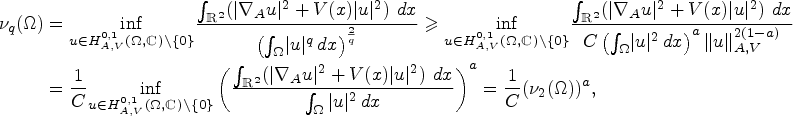
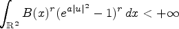
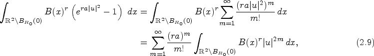
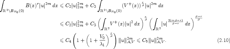
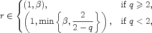
Under assumptions () and (), we can obtain that bothandare finite forand, respectively. Moreover,and can be achieved.
(i) for is a natural consequence of Lemma 2.3, so we only prove that for .
Fixed , due to the continuity of M and , there exists small enough such that
In the case of , since m is always positive, we have and there exists such that
In addition, in the case of , combining (1.8) and , there exists such that
In conclusion, using the above inequalities, we can conclude for .
(ii) It is clear that for . If , there exists a minimizing sequence such that and . Due to Lemma 2.3, up to a subsequence, we obtain that in for . It is a contradiction with the fact that .
Moreover, for , there exists a minimizing sequence such that and . Up to a subsequence, there exists such that in Furthermore, by the compact embedding , there exists a subsequence of relabeled as such that
In addition, from weakly lower semi-continuity of the norm and the definition of , we can obtain that .
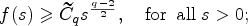
Next, we recall the following Trudinger–Moser inequality, whose proof was given in [2] (see also [13] or [20]).
Ifand, we have. Additionally, if,and, there exists a positive constantsuch that
Similar to [23, Lemmas 2.2–2.3], we have the following two lemmas for space , which are useful later.
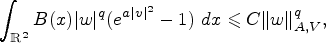
If,and, we have that
with β given in assumption ().
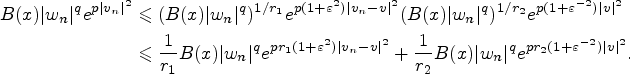
For and , it follows from that there exists such that
where has been given in assumption () and we have used the inequality
It follows from and Lemma 2.6 that
which implies we only need to estimate the first integral on the right-hand of (2.6). Noticing
similar to the proof of Lemma 2.4 (i), by () and Hölder’s inequality, we have
Consequently, due to (2.6), (2.8)–(2.10), we obtain that
which concludes the conclusion.
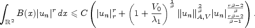
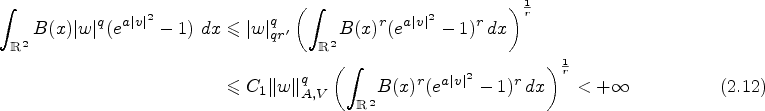
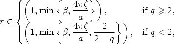
For,and any, we have
Moreover, for ζ be taken in Lemma2.1, ifand, there exists a positive constantsuch that
We choose
such that and , where . It follows from Hölder’s inequality, the continuous embedding and Lemma 2.7 that
and we have the first conclusion.
If and , we can choose
such that , and . Combining with (2.11)–(2.12) and noting , we obtain that
Due to (1.7) and (2.5), we obtain that . Moreover, we have for some positive constant M independent of v. Consequently, from and the above inequalities, it follows from and Lemma 2.6 that
which means the proof is completed.
Now, we give a similar result to Lions [29, Subsec. I.7] for our space .
Let and let be such thatis bounded in,inandfor any. Then, if, it holds
The same holds ifand.
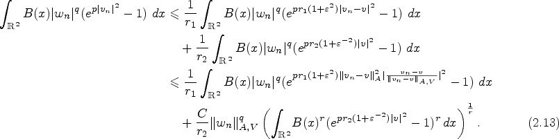
For given and , using Young’s inequality, we obtain
Thus, choosing such that , and using Young’s inequality again, we get
Because is bounded in and Lemma 2.7, the second part on the right-hand of (2.13) is bounded independently of n, which means that we only need to estimate the first part. Due to in as and for any , we get
Then by taking sufficiently close to 1 and small enough, there exists such that
Consequently, the result follows from (2.13) Lemma 2.8 and the above inequality.
Next, we give the very important monotonic conditions.
Under assumptions () and (), we have the following two statements.
The functionis increasing in. Particularly,for each.
The functionis non-decreasing in. Particularly,for each.
The proof of (i) has been given in [23], so we only prove (ii) here. Let with . From (), we obtain
which means that the function is non-decreasing in . It follows from the continuity at that is non-decreasing in .
Finally, we give a similar continuous result in [19].
Let Ω be an open subset of. Ifandsatisfies
whereis a constant, then.
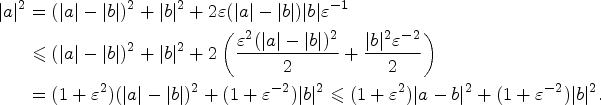
It suffices to prove that as . For given , since , there exists a such that
for all measurable subset with . Next, using the fact that , there exists such that . Let . we write
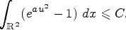
and estimate each integral separately. First, due to and , we have . In addition, by the choices made above and (2.14), we get . Finally, we claim that
Indeed, up to a subsequence, a.e. in Ω as . Moreover,
where . Consequently, the claim follows from the Lebesgue’s dominated convergence theorem.
The variational framework
We say that is a weak solution to (1.1), if for any ,
Under assumptions ()–(), it follows from (2.4), Lemma 2.8 and the continuous embedding that the following energy I to (1.1) is well defined and belongs to ,
(see the proof of Lemma 3.1 for more details). In addition, for , there holds
The functional I satisfies the Mountain Pass geometry, namely we have the following two lemmas.
Under assumptions (), ()–(), there existsuch thatif.
Fix and . If , for with , by (2.4) with , Lemma 2.8 and the continuous embedding , we get
Combining with (), we obtain that
Because of , we can choose and small enough such that . Therefore, for any with , we have
Under assumptions (), ()–(), there existssuch thatandwith ρ taken in Lemma3.1.
In virtue of the continuity of m and (1.8), there exists such that
On the other hand, in virtue of the continuity of F and (1.9), there exist such that for all , . Now choosing , there exists such that Ω contains . Integrating () and the above inequalities, we obtain that
Since and , we can conclude that as . Consequently we can take with large enough such that .
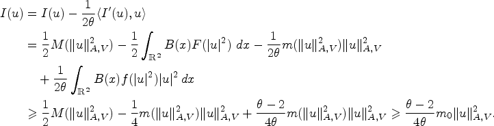
For the sake of clarity and completeness, we offer an alternative proof for the preceding lemma. By condition (), we are aware that for any . Considering (), for any , we have . Additionally, for every , we define
where defined in (). From (), we know that for ,
which means that for any , and . Thus, due to (3.1), we obtain
and as .
Under assumptions (), (), ()–(), in virtue of Lemmas 3.1–3.2, using the Mountain Pass Theorem, there exists a sequence such that
where
From Lemma 3.1, we know that .
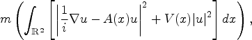
For finding the ground state state solution to equation (1.1), we consider the Nehari manifold
In addition, there is the following useful property.
Under assumptions (), (), ()–(), for fixed, there exists a uniquesuch thatand.
Defining for , we obtain that
For any and , by (2.1) with and the continuous embedding , it follows from Lemma 2.8 and for t small enough that
for t small enough. Combining with assumptions (), for t small enough, we obtain
Then, we can choose small enough such that for t small enough.
In virtue of the continuity of m and (1.8), there exists such that
as t big enough, which means that as . Consequently, there exists at least one critical point for . Due to () and (), there is a unique critical point such that . Indeed, we suppose that is the smallest critical point of and so
Under assumptions (), () and ()–(), there existsuch that
By contradiction, if , there exists a minimizing sequence such that as . Moreover, for any and , by (2.3) with , and the continuous embedding , it follows from Lemma 2.8 that
for n big enough. Combining with () and , for n big enough, we obtain that
Choosing ξ small enough such that , we obtain that
which is a contradiction with as and .
For any , according to Lemma 2.10 (i), assumptions () and , we have
The second result is a consequence of the first item.
Then, arguing as [34, Theorem 4.2] (or [32]), we have the following Lemma.
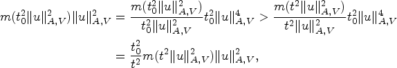
Under assumptions (), () and ()–(), we obtain that
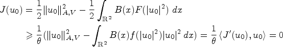
Similar to Remark 3.3, for any , we obtain that as . It follows the definition of that . Due to Lemma 3.4, there exists a unique such that and . Then, taking infimum for and due to
we can conclude that .
On the other hand, the manifold N separates into two components. According to the proof of Lemma 3.4, the component containing 0 also contains a small ball around 0. Moreover, from Lemma 3.1, Lemma 3.5 and for all , we know that for all u in this component. Consequently, any has to cross the N and .
Minimax estimates
In this section, we will give an upper estimate for the ground state energy of equation (1.1).
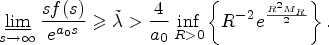
Under assumptions (), ()–() and (),.
Let be given in (). From Lemma 2.5, there exists a such that and . Due to Remark 3.3, we get that . In addition, it follows from the definition of that . In virtue of assumption (), we obtain for . Combining with (), we get
Consequently, according to the definition of , we obtain that
which completes the proof.
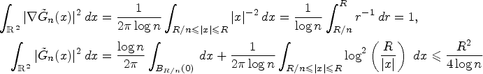
If we replace the condition () with a stronger condition (), we can take . Moreover, similar to [23], for and , we can define the following scaled and truncated Green’s functions sequence (see Moser [30]):
Next, we give some properties about the truncated Green’s functions.
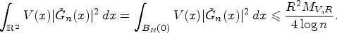
Due to Proposition 4.1, we obtain that . In addition, similar to [23, Lemma 4.2], we consider the sequence of functions and have the following technical result.
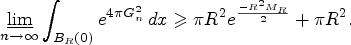
The functions sequencesatisfies that
Now, for the case that for any , we can use the previous two lemmas to obtain a similar estimate for Proposition 4.1 with the condition () rather than ().
Under assumptions (), (), ()–() and (),.
Due to Remark 3.3, we obtain as . By the definition of , we know . Because and I has the Mountain Pass geometry, there exists such that
Next, we claim that there exists at least a such that . By contradiction, if the above inequality does not hold, noting , we obtain
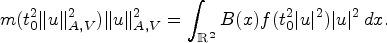
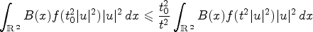
Because both B and F are nonnegative, we have . Moreover, since m is positive, we get M is an non-decreasing function, which implies that
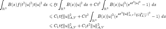
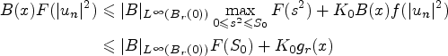
On the other hand, from , (), and the definition of , we have
It follows from as and that
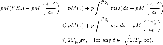
In addition, fixed , from (), there exists such that
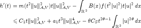
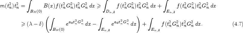
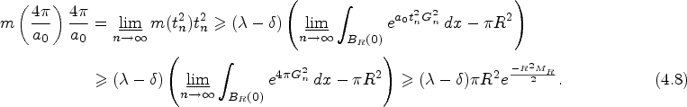
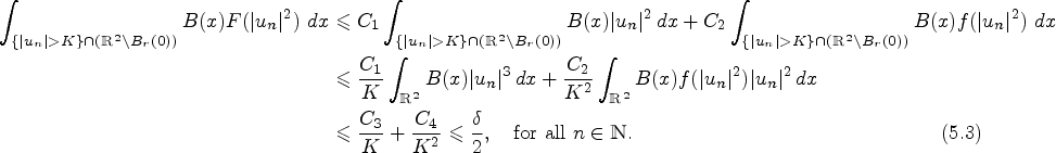
If is unbounded, there exists a subsequence of relabeled as such that as . Then, combining (1.8) and (4.3)–(4.5), for n large enough, we conclude that
which is a contradiction. Consequently, the sequence is bounded in and there exists a subsequence of relabeled as and such that . Integrating the above inequality, there exists such that for n large enough, which implies that . Combining with (4.2), we obtain that
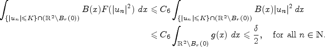
Since a.e. in as , we obtain a.e. in as , where denotes the characteristic function of . Noting in , we know
Then, it follows from the Lebesgue’s dominated convergence theorem that
Hence, combining (4.2), (4.6)–(4.7), Lemma 4.3 and the continuity of , we have
Because is arbitrary, we can let in (4.8) and get . At the end, if we take the infimum for , we will get a contradiction with (), which concludes the proof.
Proof of Theorems 1.1-1.2
In this section, we start to prove our main results. Firstly, we give the following compact conclusion.
Under assumptions (), (), ()–(), (). Ifis asequence for the energy functional I with, thenis bounded in. Moreover, up to a subsequence, there existssuch that
asfor any bounded domain;
as.
Notice is a sequence for the energy functional I, that is
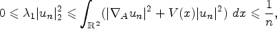
Combining with (), () and Lemma 2.10 (i), we have
with given in assumption , which means the sequence is bounded in and there exists a subsequence of relabeled as and such that in as .
Let be any bounded domain. Up to a subsequence, it follows from Lemmas 2.3–2.4 that
In addition, since is bounded in , we have as and so
From (2.1) with , for any and , there exists a constant such that
Moreover, it follows from Lemma 2.6 that
which imply that . By Lemma 2.11 and (5.1), we conclude that in as . And so
as , which proves (i).
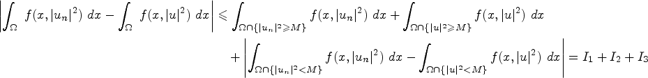
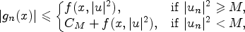
For the item (ii), taking any fixed , due to (i) and [34, Lemma A.1], there exists such that a.e. in . Then, using (), we get
for a.e. . Up to a subsequence, we have a.e. in as , by the continuity of F and the Lebesgue’s dominated convergence theorem we obatin
Thus, for proving the item (ii), it is enough to verify that, for fixed , there exists such that
It follows from that the second inequality holds for large enough. For the first inequality, we can use () and () to obtain there exist such that
Furthermore, fixed , according to the continuous embedding , the boundedness of in and (5.1), we can take K large enough such that
On the other hand, from the inequality (2.4) with , for any and with , we get , where is constant. Furthermore, because in , there exists such that a.e. in . So, by taking large enough, we obtain
Combining (5.3) and the above estimates, we conclude (5.2), which completes the proof of the item (ii).
Now, we are in position to prove Theorems 1.1–1.2.
Proof of Theorem 1.1.
In virtue of Lemmas 3.1–3.2, using the Mountain Pass Theorem, there exists a sequence such that
Due to Proposition 5.1, the sequence is bounded in , and from Lemma 2.4, there exists a subsequence of relabeled as and such that
Next, we will use the method of contradiction to prove that
Otherwise, if , then . Similar to Lemma 3.4, we define
It is clear that and . Similar to the proof of Lemmas 3.1–3.2, we know that for t small enough and as . Consequently, there exists such that
Indeed, according to Lemma 3.4, we know that is the unique critical point and . Thus, by the definition of , and Lemma 2.10 (i)–(ii), it follows from the weakly lower semi-continuity of and Fatou’s lemma that
which is a contradiction.
Finally, we will claim that and . Due to the boundedness of in , there exists such that . From the weakly lower semi-continuity of and (5.5), we obatin . If , then the proof is completed. Otherwise, if , we define
Up to a subsequence, we have that in as and . Consequently, from Lemma 2.9, we obtain
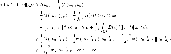
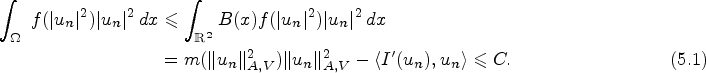
Moreover, from (5.4), (5.6), Proposition 4.1, Proposition 5.1 (ii) and assumption (), we obtain
It follows from M is monotonously increasing that . Hence, due to , we obtain that . Then, there is such that for n large enough. Furthermore, for n large enough, we can take close to and close to 1 such that and by (5.7),
Consequently, from (2.3) with , (2.7), (5.5) and (5.8), according to Hölder’s inequality and the continuous embedding , we conclude that
Combining with , and in , we obtain
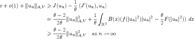
which is a contradiction. Thus, we get that and so . Combining and (5.4), we have and . Recalling that Lemma 3.6, is a ground state solution.
Proof of Theorem 1.2.
In this case, . Using Proposition 4.4 instead of Proposition 4.1, similar to the proof of the Theorem 1.1, we can draw the conclusion.
The proof of Theorems 1.3-1.4
In the final section, we consider the local case. From now on, we always assume that , which means equation (1.1) becomes the following Schrödinger equation (1.4)
We say that is a weak solution to (1.4), if for any ,
Under assumptions ()–(), it follows from (2.4), Lemma 2.8 and the continuous embedding that the following energy J is well defined and belongs to ,
Moreover, for , there holds
Similar to Lemmas 3.1–3.2, we can prove that J satisfies the Mountain Pass geometry and there exists a sequence such that
where
For finding the ground state solution to equation (1.4), we consider the Nehari manifold
Using ()–() and (), for each fixed , we define and have
Similar to the proof of Lemma 3.4 and Lemma 3.6, due to is non-decreasing in , we obtain that there exists such that
Similar to Proposition 4.1 and Proposition 4.4, we have the following estimates for .
The following statements are true.
Under assumptions ()–() and (),.
Under assumptions (), ()–() and (),.
And similar to Proposition 5.1, we have
Under assumptions ()–() and (). Ifis asequence for the energy functional J with, thenis bounded in. Moreover, up to a subsequence, there existssuch that
asfor any bounded domain;
as.
Notice is a sequence for the energy functional J, that is
Combining with (), we have
with given in assumption (), which means that the sequence is bounded in . The rest proof is similar to the proof of Proposition 5.1, so we omit it here.
Now, we are in position to prove Theorems 1.3–1.4.
Proof of Theorem 1.3.
Since J satisfies the Mountain Pass geometry, we can obtain there exists a sequence such that
By Proposition 6.2, we obtain the sequence is bounded in , and from Lemma 2.4 there exists a subsequence of relabeled as and such that
Next, up to a subsequence, we claim that for any ,
Up to a subsequence, from (6.2), we have that a.e. in as and so there exists such that a.e. in . Due to Proposition 6.2 (i), we know
and from [34, Lemma A.1] there exists such that a.e. in . Thus, for any , we have for a.e. with
Using the Lebesgue’s convergence dominated theorem, we can get (6.3). Furthermore, according to (6.1)–(6.3), we obtain that
Due to the argument of Lemma 2.3, we know that is dense in , from which we obtain . In addition, due to (), we have that
with taken in assumption (). Consequently, we can use the estimate that and proceed as in the proof of Theorem 1.1.
Proof of Theorem 1.4.
In this case, . Using the estimate rather than , similar to the proof of theorem of Theorem 1.3, we can get the ideal result.
Footnotes
Acknowledgements
This research was partially supported by the NSFC (12071192, 12371242) and Natural Science Foundation of Gansu Province of China (22JR5RA473).
AlvesC.O.CassaniD.TarsiC.YangM., Existence and concentration of ground state solutions for a critical nonlocal Schrödinger equation in , J. Differential Equations261 (2016), 1933–1972. doi:10.1016/j.jde.2016.04.021.
3.
AlvesC.O.CorrêaF.J.S.A.FigueiredoG.M., On a class of nonlocal elliptic problems with critical growth, Differ. Equ. Appl.2 (2010), 409–417.
4.
AlvesC.O.FigueiredoG.M.FurtadoM.F., Multiple solutions for a nonlinear Schrödinger equation with magnetic fields, Comm. Partial Differential Equations36 (2011), 1565–1586. doi:10.1080/03605302.2011.593013.
5.
AmbrosioV., On a fractional magnetic Schrödinger equation in R with exponential critical growth, Nonlinear Anal.183 (2019), 117–148. doi:10.1016/j.na.2019.01.016.
6.
AmbrosioV.d’AveniaP., Nonlinear fractional magnetic Schrödinger equation: Existence and multiplicity, J. Differential Equations264(5) (2018), 3336–3368. doi:10.1016/j.jde.2017.11.021.
7.
ArioliG.SzulkinA., A semilinear Schrödinger equation in the presence of a magnetic field, Arch. Ration. Mech. Anal.170 (2003), 277–295. doi:10.1007/s00205-003-0274-5.
8.
BarileS.CingolaniS.SecchiS., Single-peaks for a magnetic Schrödinger equation with critical growth, Adv. Differential Equations11 (2006), 1135–1166.
9.
BarileS.FigueiredoG.M., An existence result for Schrödinger equations with magnetic fields and exponential critical growth, J. Elliptic Parabol. Equ.3 (2017), 105–125. doi:10.1007/s41808-017-0007-9.
10.
BégoutP.SchindlerI., On a stationary Schrödinger equation with periodic magnetic potential, Rev. R. Acad. Cienc. Exactas Fís. Nat. Ser. A Mat. RACSAM115 (2021), 72, 32 pp. doi:10.1007/s13398-020-00970-9.
11.
BernsteinS., Sur une classe d’équations fonctionelles aux dérivées partielles, Bull. Acad. Sci. URSS. Sér.4 (1940), 17–26.
12.
BrezisH., Functional Analysis, Sobolev Spaces and Partial Differential Equations, Universitext, Springer, New York, 2011.
13.
CaoD.M., Nontrivial solution of semilinear elliptic equation with critical exponent in , Comm. Partial Differential Equations17 (1992), 407–435. doi:10.1080/03605309208820848.
14.
ChenC.Y.KuoY.C.WuT.F., The Nehari manifold for a Kirchhoff type problem involving sign-changing weight functions, J. Differential Equations250 (2011), 1876–1908. doi:10.1016/j.jde.2010.11.017.
15.
CingolaniS., Semiclassical stationary states of nonlinear Schrödinger equations with an external magnetic field, J. Differential Equations188 (2003), 52–79. doi:10.1016/S0022-0396(02)00058-X.
16.
CingolaniS.SecchiS., Semiclassical states for NLS equations with magnetic potentials having polynomial growths, J. Math. Phys.46 (2005), 053503. 19 pp.
17.
d’AveniaP.JiC., Multiplicity and concentration results for a magnetic Schrödinger equation with exponential critical growth in , Int. Math. Res. Not. IMRN2022 (2022), 862–897. doi:10.1093/imrn/rnaa074.
18.
d’AveniaP.JiC., Semiclassical states for a magnetic nonlinear Schrodinger equation with exponential critical growth in , J. Anal. Math. (2023). doi:10.1007/s11854-023-0312-1.
19.
de FigueiredoD.G.MiyagakiO.H.RufB., Elliptic equations in with nonlinearities in the critical growth range, Calc. Var. Partial Differential Equations3 (1995), 139–153. doi:10.1007/BF01205003.
20.
do ÓJ.M., N-Laplacian equations in with critical growth, Abstr. Appl. Anal.2 (1997), 301–315. doi:10.1155/S1085337597000419.
21.
EstebanM.J.LionsP.L., Stationary solutions of nonlinear Schrödinger equations with an external magnetic field, in: Partial Differential Equations and the Calculus of Variations I, Progr. Nonlinear Differential Equations Appl., Vol. 1, Birkhäuser Boston, Boston, 1989, pp. 401–449.
22.
FengB.H.WangD.-B.WuZ.-G., Infinitely many localized semiclassical states for nonlinear Kirchhoff-type equation, Adv. Nonlinear Anal.12(1) (2023), 20220296. doi:10.1515/anona-2022-0296.
23.
FurtadoM.F.ZanataH.R., Kirchhoff–Schrödinger equations in with critical exponential growth and indefinite potential, Commun. Contemp. Math.23 (2021), 2050030. doi:10.1142/S0219199720500303.
24.
GraefJ.R.HebboulD.MoussaouiT., Existence of positive radial solutions to a p-Laplacian Kirchhoff type problem on the exterior of a ball, Opuscula Math.43(1) (2023), 47–66. doi:10.7494/OpMath.2023.43.1.47.
25.
KirchhoffG., Mechanik, Teubner, Leipzig, 1883.
26.
LiQ.YangZ.D., Multiple solutions for N-Kirchhoff type problems with critical exponential growth in , Nonlinear Anal.117 (2015), 159–168. doi:10.1016/j.na.2015.01.005.
27.
LiangS.ShiS., On multi-bump solutions of nonlinear Schrödinger equation with electromagnetic fields and critical nonlinearity in , Calc. Var. Partial Differential Equations56 (2017), 25, 29 pp. doi:10.1007/s00526-017-1110-3.
28.
LiebE.H.LossM., Analysis, 2nd edn, Graduate Studies in Mathematics, Vol. 14, American Mathematical Society, Providence, 2001.
29.
LionsP.L., The concentration-compactness principle in the calculus of variations. The limit case, part 1, Rev. Mat. Iberoamericana1 (1985), 145–201. doi:10.4171/rmi/6.
30.
MoserJ., A sharp form of an inequality by N. Trudinger, Indiana Univ. Math. J.20 (1971), 1077–1092. doi:10.1512/iumj.1971.20.20101.
31.
PohožaevS.I., On a class of quasilinear hyperbolic equations, Math. USSR Sbornik25 (1975), 145–158. doi:10.1070/SM1975v025n01ABEH002203.
32.
RabinowitzP.H., Minimax Methods in Critical Point Theory with Applications to Differential Equations, Reg. Conf. Ser. Math., American Mathematical Society, 1986.
33.
SirakovB., Existence and multiplicity of solutions of semi-linear elliptic equations in , Calc. Var. Partial Differential Equation11 (2000), 119–142. doi:10.1007/s005260000010.
34.
WillemM., Minimax Theorems, Springer Science & Business Media, 1997.
35.
WuY.ChenP., Ground state solutions for magnetic Schrödinger equations with polynomial growth, Adv. Nonlinear Anal.13(1) (2024), 20240011. doi:10.1515/anona-2024-0011.
36.
XiangM.Q.PucciP.SquassinaM.ZhangB.L., Nonlocal Schrödinger-Kirchhoff equations with external magnetic field, Discrete Contin. Dyn. Syst. Ser. A37 (2017), 503–521.