In this paper, we embark on a captivating exploration of the stabilization of locally transmitted problems within the realm of two interconnected wave systems. To begin, we wield the formidable Arendt-Batty criteria (Trans. Am. Math. Soc.306(2) (1988) 837–852) to affirm the resolute stability of our system. Then, with an artful fusion of a frequency domain approach and the multiplier method, we unveil the exquisite phenomenon of exponential stability, a phenomenon that manifests when the waves of the second system synchronize their propagation speeds. In cases where these speeds diverge, our investigation reveals a graceful decay of our system’s energy, elegantly characterized by a polynomial decline at a rate of .
When a vibrating source disturbs the first particle of a medium, a wave is generated. This phenomenon propagates from particle to particle through the medium, typically modeled by a wave equation. To mitigate these vibrations, the most common approach is the addition of damping.
In recent years, the stabilization of wave systems, whether simple or coupled, with localized damping has garnered significant attention from researchers, particularly in the one-dimensional case (see [1,4–6,17,19,24,25]). Notably, in two papers, it was demonstrated that the smoothness of the damping and coupling coefficients plays a crucial role in the stability and regularity of the solutions of the studied systems. Specifically, in [2], Akil, Badawi, and Nicaise investigated the stability of locally coupled wave equations with local Kelvin–Voigt damping when the supports of the damping and coupling coefficients are disjoint. They showed that the energy of their system decays polynomially, with rates of and in different cases.
Additionally, there are numerous publications on the multi-dimensional setting (see [3,7–14,20,22,23,27–29,32,34]). Our objective in this work is to examine a more general problem. However, before presenting our main contributions, let us first recall some previous results for such systems. In 2020, S. Gerbi et al. [18] proved the exponential decay rate of solutions when the waves propagate with equal speeds, the coupling region is a subset of the damping region, and it satisfies the geometric control condition (GCC), with the damping and coupling coefficients in . Similarly, Wehbe, Ibtissam, and Akil [33] recently showed that the energy of smooth solutions of the system decays polynomially, at a rate of , considering both the damping and coupling coefficients are non-smooth. They extended this work to the multidimensional case in [8], studying the stability of the system under various geometric control conditions. They established polynomial stability when there is an intersection between the damping and coupling regions, and also when the coupling region is a subset of the damping region under the GCC.
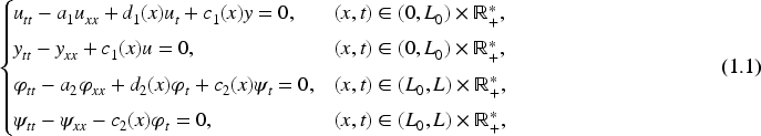
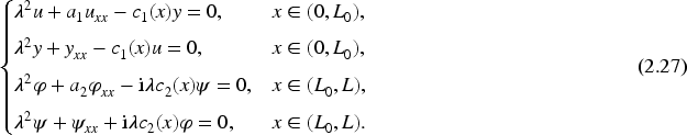
Within the intricate framework of this paper, our focus converges on an intriguing question: What specific qualities define the stability of our transmission problems (1.1)? Indeed, this problem involves two wave systems: one weakly coupled and the other strongly coupled with non-smooth coefficients. To the best of our knowledge, no results exist in the literature concerning our problem (1.1), especially in the one-dimensional case. The goal of this paper is to address this gap by studying the stability of the following locally transmitted problem:
with fully Dirichlet boundary conditions,
and the following transmission conditions,
and with the following initial data
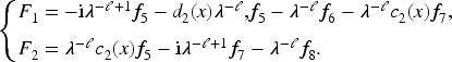
where
and , , , are strictly positives constants, , with
where denotes the Poincaré constant. More precisely, is the smallest positive constant such that
The paper is structured as follows: First in Section 2, we prove the well-posedness of our system by using semigroup approach. Then in Section 2.1, following a general criteria of Arendt and Batty, we show the strong stability of our problem. Next, in Section 2.2, by using the frequency domain approach combining with a specific multiplier method, we establish exponential stability of the solution if and only if the waves of the second coupled equations have the same speed of propagation (i.e., ). In the case when , we prove that the energy of our problem decays polynomially with the rate .
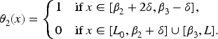
Geometric description of the functions , , and .
.Well-posedness and stability results
Let’s start by rigorously establishing the well-posedness of the system (1.1)–(1.4) using a detailed semi-group approach.
Case1. If in .
Let be a regular solution of the system (1.1)–(1.4). The energy of the system is given by
A straightforward computation gives
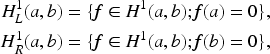
Thus, the system (1.1)–(1.4) is dissipative in the sense that its energy is a non increasing function with respect to the time variable t. We introduce the following Hilbert spaces
for any real numbers a, b such that . The energy space is now defined by
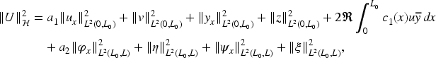
equipped with the following norm
for all .
Let , it’s easy to see that problem (1.1)–(1.4) is formally equivalent to the following abstract evolution equation in the Hilbert space
and the unbounded operator is defined by
for all , with domain
The unbounded linear operatorgenerates a-semigroup of contractions on.
Using Lumer–Phillips theorem (see [30]), it is sufficient to prove that is a maximal dissipative operator so that generates a C0-semigroup of contractions on . First, let . Then, integrating by parts we have
This implies that is dissipative. Now, let us go on with maximality. Let , we look for solution of
Multiplying (2.9), (2.16) by and (2.11), (2.17) by , integrating over , we get
and
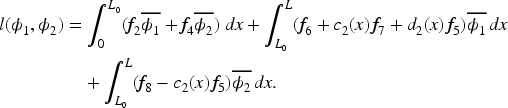
Adding the above equations, we obtain the following variational problem:
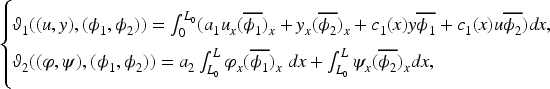
where
with
and
First, thanks to (1.7) we have that is a bilinear, continuous and coercive form on . Second it’s easy to see that is a bilinear, continuous and coercive form on and l is linear continuous form on . Then, using Lax–Milgram theorem, we deduce that there exists unique solution of the variational problem (2.22). By using the classical elliptic regularity we deduce that and . Next by setting , , and , we deduce that is solution of (2.7). To conclude, we need to show the uniqueness of such a solution. So, let be a solution of (2.7) with
Then we directly deduce that and therefore satisfies (2.22) with and satisfies (2.22) with . As , are two sesquilinears, continuous coercive forms, we deduce that
In other words, . Consequently, we get is a unique solution of (2.7).
Since the resolvent set of we easily get for a sufficiently small (see [26, Thm. 1.2.4]). This, together with the dissipativeness of , imply that is dense in (see [30, Thm. 4.6]). Then is m-dissipative in .
As generates a -semigroup of contractions , we have the following result:
(Existence and uniqueness of the solution)
If, then problem (2.4) admits a unique strong solution U satisfying:
If, then problem (2.4) admits a unique weak solution U satisfying:
Strong stability
Now the following result is about the strong stability of system (1.1)–(1.4)
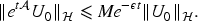
The-semigroup of contractionsis strongly stable in the energy spacein the sense that
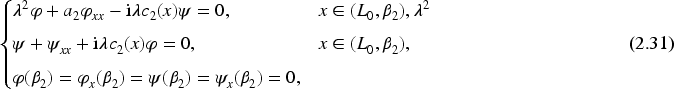
Since the resolvent of is compact in , it follows from the Arendt–Batty’s theorem (see [15]) that the system (1.1)–(1.4) is strongly stable if and only if does not have pure imaginary eigenvalues, i.e. . From Proposition 2.1, we have that . Therefore, only must be proved. For this purpose, suppose that there exists a real number and such that
Detailing (2.23) and using (2.25), we get the following equations
and
Our goal is to prove that in and in . For simplicity, we divide the proof into two steps.
Step 1. The aim of this step is to show that in . So, using (2.25) and the third equation in (2.26), we have
From (2.27)3, (1.6) and the above equation, we get
Using the above result and (2.28), we have in . Since , then
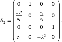
Let , the following system
can be written as
where
The solution of the differential equation (2.32) is given by
Then,
Now, we still need to prove that in and in . Using (2.28), (2.29), the fact that , and the equations (2.27)3 and (2.27)4, we get the following systems:
and
Then, using Holmgren uniqueness theorem, we get
Hence from (2.28), (2.29), (2.34) and the above result, we obtain
Step2. The aim of this step is to show that in . From (2.38) and the fact that φ, , we have the following boundary condition
Let . From (2.43), . The system (2.44) can be written as the following equation
where
The solution of the differential equation (2.45) is given by
Then,
Now, we still need to show that in . Using the above result, the fact that and the equations (2.27)1 and (2.27)2, we get:
and
Again, using Holmgren uniqueness theorem, we have
Finally, by using (2.26), (2.38), (2.42), (2.47) and (2.50) we deduce that in and we reached our disered result.
Exponential and polynomial stability
In this section, we will study the exponential and polynomial stabilities of the system (1.1)–(1.4). Our main result in this part is the following theorems.
If, then the C0-semigroupis exponentially stable; i.e., there exists constantsandindependent ofsuch that
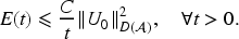
If, then there existssuch that for every, we have
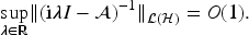
Since (see Section 2.1), according to Huang [21], Prüss [31], Borichev and Tomilov [16], to proof Theorems 2.4 and 2.5, we still need to check if the following condition hold:
We will prove condition (2.51) by an argument of contradiction. For this purpose, suppose that (2.51) is false, then there exists with
such that
For simplicity, we drop the index n. Equivalently, from (2.53), we have
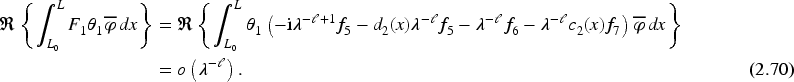
Here we will check the condition (2.51) by finding a contradiction with (2.52) by showing . From (2.52), (2.54), (2.56), (2.58) and (2.60), we obtain
and
For clarity, we will divide the proof into several lemmas.
The solutionof (2.54)–(2.61) satisfies the following asymptotic behavior estimation
Taking the inner product of (2.53) with U in and using (2.6), we get
Thus, from the above equation, the fact that and , we obtain the first estimation in (2.64). By using (2.58) and the first estimation in (2.64), we get the last estimation.
Inserting (2.58) and (2.60) into (2.59) and (2.61), we get the following system
where
Let. The solutionof (2.54)–(2.61) satisfies the following asymptotic behavior estimation
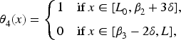
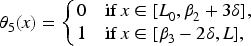
First, we define the cut-off function by
Multiplying (2.65) by , integrating over and taking the real part, we get
Using the fact that in and is uniformly bounded in , we obtain
On the other hand, using Lemma 2.6, the fact that and are uniformly bounded in and the definition of , we get
and
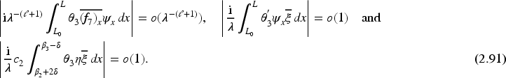
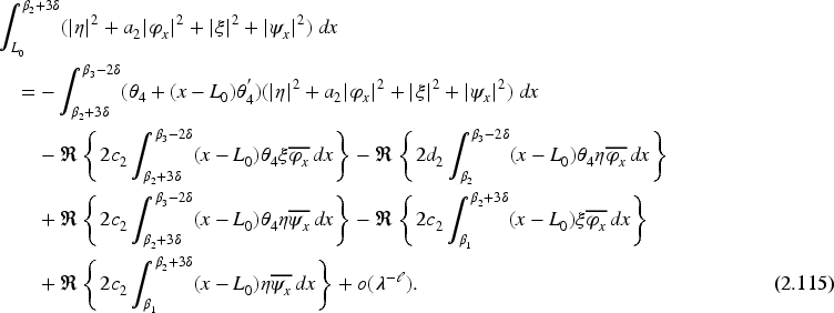
Furthermore, using Lemma 2.6 and the definition of the function in (2.68), we get
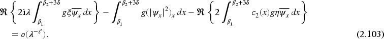
Multiplying the above equations by and respectively, integrating over , taking the real part, then using the fact that , ξ are uniformly bounded in in particular in , and , we have
and
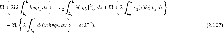
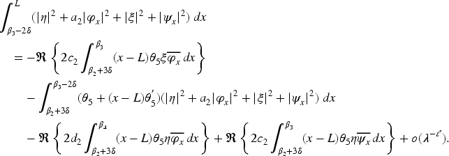
Adding (2.102) and (2.103), then using integration by parts, we obtain
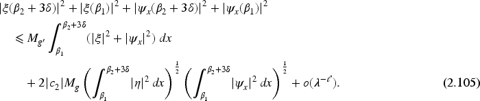
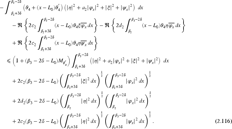
Using the definition of g and Cauchy–Schwarz inequality in the above equation, we obtain
Finally, from (2.105) and the fact that , ξ and η are uniformly bounded in in particular in , we have the second estimation (2.96).
Letbe a function with. The solutionof (2.54)–(2.61) satisfies the following asymptotic behavior estimation
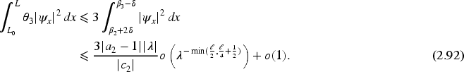
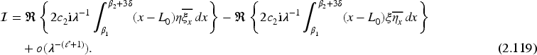
Multiplying (2.59) by , integrating over , taking the real part, then using the fact that is uniformly bounded in and , we get
Inserting the above equations in (2.118), then using the fact that η and ξ are uniformly bounded in and , , we obtain
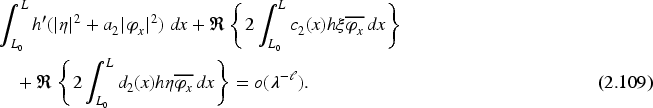
Using integration by parts to the second term in the above equation, we obtain
From Lemma 2.11, we deduce that
Using Cauchy–Schwarz inequality, (2.121), (2.122) and the fact that η, ξ are uniformly bounded in , we obtain
and
Inserting the above estimations in (2.120), we get
Finally, from the above estimation and (2.117), we obtain the desired estimation (2.113). Next, using the result of Lemma 2.12 with , we obtain
Using Cauchy–Schwarz inequality in the above equation, we get
Thus, from the above inequality, Lemmas 2.6–2.9 and the fact that , , ξ are uniformly bounded in , we get (2.114).
Let. The solutionof (2.54)–(2.61) satisfies the following estimate
where.
The proof is split into two steps.
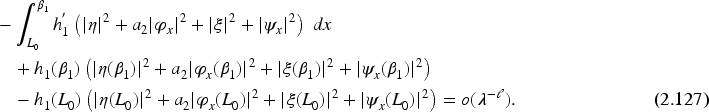
Step 1. Letting , the following estimate is targeted to prove
First, multiplying (2.59) and (2.61) by and respectively, integrating over , taking the real part, then using the fact that and are uniformly bounded in in particular in and , , we obtain
Inserting the above equations in (2.128) and (2.129), then using the fact that η and ξ are uniformly bounded in in particular in and , , we get
and
Adding (2.130) and (2.131), then using integration by parts, we get (2.127).
Step2. Taking in (2.127) and using (2.113), we obtain
Using (2.58), (2.60) and the transmission conditions (1.3), we get (2.126).
Let. The solutionof (2.54)–(2.61) satisfies the following estimate
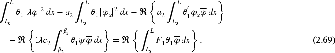
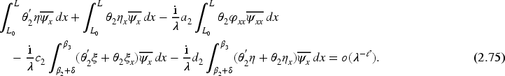
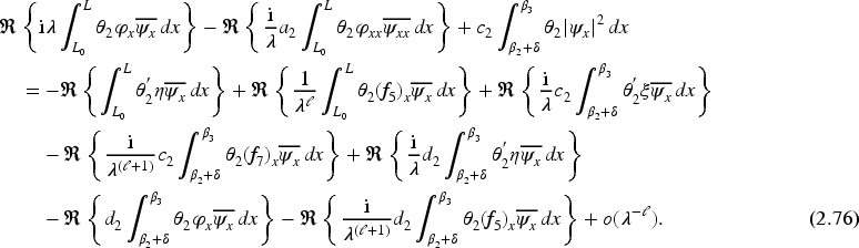
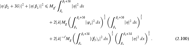
First, using the multipliers and for (2.55) and (2.57) respectively, integrating over , taking the real part, then using the fact that and are uniformly bounded in and , , we obtain
and
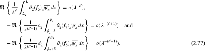
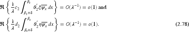
Using Cauchy–Schwarz inequality, the fact that , , , are uniformly bounded in , we get
Inserting the above equations in (2.137) and (2.138), then using the fact that v and z are uniformly bounded in and , , we get
and
Adding (2.139) and (2.140), then using integration by parts, we obtain
Using the above result and (2.126), we get (2.133).
Proof of Theorem 2.4.
The proof of Theorem 2.4 is divided into three steps.
Step 1. By taking and in Lemmas 2.6–2.9, we obtain
Consequently, we have
Step 2. Using the fact that in Lemmas 2.13 and 2.15, we obtain
and
Step 3. According to Step 1 and Step 2, we obtain , which contradicts (2.52). This implies that
So by Theorem A.3, we deduce that system (1.1)–(1.4) is exponentially stable.
Proof of Theorem 2.5.
The proof of Theorem 2.5 is divided into three steps.
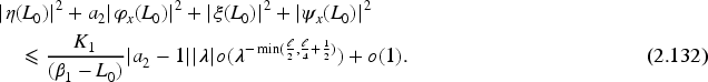
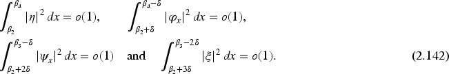
Step 1. Taking , then from Lemmas 2.8 and 2.9, we get
Taking in the above estimations, we obtain
Taking in Lemma 2.6 and 2.7, we get
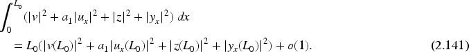
In particular, we have
Step 2. Using the fact that and , then from Lemmas 2.13 and 2.15, we obtain
and
Step 3. According to Step 1 and Step 2, we obtain , which contradicts (2.52). This implies that
So by Theorem A.4, we deduce that system (1.1)–(1.4) is polynomially stable.
.Conclusion and future works
We have studied the stabilization of a locally transmission problems of two wave systems. We proved the strong stability of the system by using Arendt and Batty criteria. We established the exponential stability of the solution if and only if the waves of the second coupled equations have the same speed propagation (i.e., ). In the case , we proved that the energy of our problem decays polynomially with the rate . Finally, we present some open problems:
Prove that the energy decay rate is optimal.
Study system (1.1)–(1.4) in the multidimensional case.
Can we get stability results if in .
Footnotes
To make this paper more self-contained, we provide a brief appendix that recalls some key concepts and stability results used in this work.
To show the strong stability of a C0-semigroup of contraction we rely on the following result due to Arendt–Batty [15].
Concerning the characterization of exponential stability of a C0-semigroup of contraction we rely on the following result due to Huang [21] and Prüss [31].
Also, concerning the characterization of polynomial stability of a C0-semigroup of contraction we rely on the following result due to Borichev and Tomilov [16].
References
1.
AkilM., Stability of piezoelectric beam with magnetic effect under (Coleman or Pipkin) – Gurtin thermal law, Zeitschrift für angewandte Mathematik und Physik73(6) (2022), 236. doi:10.1007/s00033-022-01867-w.
2.
AkilM.BadawiH.NicaiseS., Stability results of locally coupled wave equations with local Kelvin–Voigt damping: Cases when the supports of damping and coupling coefficients are disjoint, Computational and Applied Mathematics41 (2022), 240.
3.
AkilM.BadawiH.NicaiseS.RégnierV., Stabilization of coupled wave equations with viscous damping on cylindrical and non-regular domains: Cases without the geometric control condition, Mediterr. J. Math.19 (2022), 271. doi:10.1007/s00009-022-02164-6.
4.
AkilM.BadawiH.NicaiseS.WehbeA., Stability results of coupled wave models with locally memory in a past history framework via nonsmooth coefficients on the interface, Math. Methods Appl. Sci.44(8) (2021), 6950–6981. doi:10.1002/mma.7235.
5.
AkilM.BadawiH.WehbeA., Stability results of a singular local interaction elastic/viscoelastic coupled wave equations with time delay, Commun Pure Appl Anal20(9) (2021), 2991–3028. doi:10.3934/cpaa.2021092.
6.
AkilM.GhaderM.WehbeA., The influence of the coefficients of a system of wave equations coupled by velocities on its stabilization, SeMA78 (2021), 287–333. doi:10.1007/s40324-020-00233-y.
7.
AkilM.HajjejZ., Exponential stability and exact controllability of a system of coupled wave equations by second order terms (via Laplacian) with only one non-smooth local damping, Mathematical Methods in the Applied Sciences47 (2024), 1883–1902.
8.
AkilM.IssaI.WehbeA., A N-dimensional elastic/viscoelastic transmission problem with Kelvin–Voigt damping and non smooth coefficient at the interface, SeMA80 (2023), 425–462. doi:10.1007/s40324-022-00297-y.
9.
AkilM.WehbeA., Stabilization of multidimensional wave equation with locally boundary fractional dissipation law under geometric conditions, Math. Control Relat. Fields8 (2018), 1–20. doi:10.3934/mcrf.2018001.
10.
AkilM.WehbeA., Indirect stability of a multidimensional coupled wave equations with one locally boundary fractional damping, 2021.
11.
Alabau-BoussouiraF., Indirect boundary stabilization of weakly coupled hyperbolic systems, Mathematics SIAM J. Control. Optim.41 (2002), 511–541.
12.
Alabau-BoussouiraF., A two-level energy method for indirect boundary observability and controllability of weakly coupled hyperbolic systems, SIAM J. Control. Optim.42 (2003), 871–906.
13.
Alabau-BoussouiraF.LéautaudM., Indirect controllability of locally coupled wave-type systems and applications, Mathematics (2013).
14.
Ali WehbeN.N.NasserR., Stability of n-d transmission problem in viscoelasticity with localized Kelvin–Voigt damping under different types of geometric conditions, Math. Control Relat. Fields11(4) (2021), 885–904. doi:10.3934/mcrf.2020050.
15.
ArendtW.BattyC.J.K., Tauberian theorems and stability of one-parameter semigroups, Trans. Am. Math. Soc.306(2) (1988), 837–852. doi:10.1090/S0002-9947-1988-0933321-3.
16.
BorichevA.TomilovY., Optimal polynomial decay of functions and operator semigroups, Math. Annal.347(2) (2009), 455–478. doi:10.1007/s00208-009-0439-0.
17.
BoutaayamouI.FragnelliG.MugnaiD., Boundary controllability for a degenerate wave equation in non divergence form with drift, submitted, 33 pages, arXiv:2109.1253.
18.
GerbiS.KassemC.MortadaA.et al., Exact controllability and stabilization of locally coupled wave equations: Theoretical results, Zeitschrift für Analysis und ihre Anwendungen40 (2021), 67–96. doi:10.4171/zaa/1673.
19.
HassineF.SouayehN., Stability for coupled waves with locally disturbed Kelvin–Voigt damping, 2019, arXiv:1909.09838.
20.
HayekA.NicaiseS.SalloumZ.WehbeA., A transmission problem of a system of weakly coupled wave equations with Kelvin–Voigt dampings and non-smooth coefficient at the interface, SeMA J.77(3) (2020), 305–338. doi:10.1007/s40324-020-00218-x.
21.
HuangF.L., Characteristic conditions for exponential stability of linear dynamical systems in Hilbert spaces, Ann. Differ. Equ.1(1) (1985), 43–56.
22.
LebeauG., Équation des ondes amorties, in: Algebraic and Geometric Methods in Mathematical Physics (Kaciveli, 1993), Mathematical Physics Studies, Vol. 19, Kluwer Academic Publishers, Dordrecht, 1996.
23.
LebeauG., Équations des ondes amorties, Séminaire Équations aux dérivées partielles (Polytechnique), 1993–1994, talk:15.
24.
LiuK., Locally distributed control and damping for the conservative systems, SIAM J. Control Optim.35(5) (1997), 1574–1590. doi:10.1137/S0363012995284928.
25.
LiuZ.RaoB., Characterization of polynomial decay rate for the solution of linear evolution equation, Z. Angew. Math. Phys.56(4) (2005), 630–644. doi:10.1007/s00033-004-3073-4.
26.
LiuZ.ZhengS., Semigroups Associated with Dissipative Systems, Research Notes in Mathematics, Vol. 398, Champman and Hall/CRC.
27.
NajdiN., Study of the exponential and polynomial stability of some systems of coupled equations with indirect bounded or unbounded control, PhD thesis, 2016.
28.
NasserR.NounN.WehbeA., Stabilization of the wave equations with localized Kelvin-Voigt type damping under optimal geometric conditions, C. R. Math.357(3) (2019), 272–277. doi:10.1016/j.crma.2019.01.005.
29.
NicaiseS.PignottiC., Stability of the wave equation with localized Kelvin–Voigt damping and boundary delay feedback, Discret. Contin. Dyn. Syst. Ser9(3) (2016), 791–813. doi:10.3934/dcdss.2016029.
30.
PazyA., Semigroups of Linear Operators and Applications to Partial Differential Equations, Applied Mathematical Sciences, Vol. 44, Springer-Verlag, New York, 1983.
31.
PrüssJ., On the spectrum of C0-semigroups, Trans. Am. Math. Soc.284(2) (1984), 847–857. doi:10.2307/1999112.
32.
TebouL., A constructive method for the stabilization of the wave equation with localized Kelvin–Voigt damping, Comptes Rendus Math.350 (2012), 603–608. doi:10.1016/j.crma.2012.06.005.
33.
WehbeA.IssaI.AkilM., Stability results of an elastic/viscoelastic transmission problem of locally coupled waves with non smooth coefficients, Acta Appl. Math.171(1) (2021), 1–46. doi:10.1007/s10440-021-00384-8.
34.
WehbeA.YoussefW., Indirect locally internal observability of weakly coupled wave equations, Differential Equations and Applications – DEA3(3) (2011), 449–462. doi:10.7153/dea-03-28.