Model calibration of a long-span concrete cable-stayed bridge based on structural health monitoring data: Influence of concrete variability

Abstract

Structural Health Monitoring (SHM) systems, in combination with controlled load tests, can provide valuable data for calibrating high fidelity bridge models, which can then be used for evaluating the long-term performance of the bridge, improved load ratings, and permit vehicle evaluation. The objective of this research was to calibrate a 3D model of the Indian River Inlet (IRIB) cable-stayed bridge, using strains recorded by the bridge SHM system during a controlled load test. The bridge was modeled in STAAD-Pro and calibrated using a pre-commercialized software platform that uses a Generic Algorithm to minimize the error between the measured and predicted strains. The calibration parameters were the elastic modulus of groups of the main longitudinal edge girder/deck elements, which once calibrated, could be related to the measured concrete strength of the members. Four different models were investigated, using 6, 10, 14, and 18 parameter element groups of the edge girder members. Of the different models, the 14 and 18 parameter models yielded the best results. The “design” model yielded errors as high as 42% when compared to the measured strains; the error was less than 10% for the majority of measurements for the 14-parameter model. Including the effect of the traffic barriers in the model, the weighted average concrete strength of the calibrated model was within 4% of the measured weighted strength. The calibration was shown to be insensitive to measurement noise and was validated using several unique single and multi-vehicle load cases that were heavier and more offset from the centerline of the bridge. The calibration procedure was able to capture the variability in flexural stiffness of the edge girders due to the variability of the concrete, resulting in significantly better agreement between the live load measured strains and the model predicted strains.

Keywords

Calibration cable-stayed bridge concrete concrete strength strain load test structural health monitoring system identification

1 Introduction

System Identification (SI), sometimes also called model updating, has long been a topic of intense research aimed at developing robust, efficient, and cost-effective methods for identifying model parameters using the measured response of a structure. While the concept has been around for some time, very early efforts were constrained by limits on the memory and processing speed of computers, and the expense and effort that was required to instrument and test large civil infrastructure. However, with the advances that have been made in computers it is now possible to develop and “calibrate” high-fidelity structural models, much more easily. SI algorithms have become more sophisticated, with the ability to handle many model parameters and many response inputs. Advances in sensors and computers have also streamlined and simplified the input side of the SI problem. Today it is much easier to deploy sensors on a structure and measure either static, or dynamic data – thus the tremendous interest in Structural Health Monitoring (SHM). The convergence of advances in model updating and SHM hold the potential of real benefit in the design, maintenance, operation, and repair of civil infrastructure.

To take advantage of the near real-time, continuous data that SHM systems can provide today, and the benefit to be derived from a model that is calibrated using the data, an automated calibration method is needed that will streamline and simplify the process. Only then will SHM and model calibration move from a mostly research/academic pursuit, to state-of-the-practice, where these modern tools will be in the hands of practicing engineers and owners. The focus of this paper is on the automated model calibration or system identification (SI) of a long-span cable-stayed, concrete bridge, using data from a permanent SHM system on the bridge. The paper also illustrates the influence of concrete variability on modeling of a long-span concrete cable-stayed bridge.

Hart and Yao [1] provided one of the early surveys of research on SI. Their focus was on SI in structural engineering, with applications geared towards earthquake engineering. In 1993, a comprehensive summary of research conducted through the early ‘90’s was provided by Mottershead and Friswell [2]. Their survey is quite extensive, includes well over 200 references, and spans the range of SI discipline areas. More recently, the ASCE Committee on Structural Identification of Constructed Systems published a monograph on SI of constructed systems [3]. The report is much more than just a literature review, as it covers methods for system identification of structures, outlines a systematic procedure for carrying out the analysis, and provided a series of case studies with results.

Early applications of SI typically relied on determining the dynamic properties of a structure from an ambient vibration survey, a forced harmonic vibration test, or an impulse response test. Recent examples of investigations that rely on dynamic measurements include Ribeiro et al. [4], Jang et al. [5], Garcia-Palencia et al. [6], Zhang et al. [7], Dubbs and Moon [8], and Whelan et al. [9].

Until recently, measuring strain, tilt, or displacement of a civil structure was not so easy. However, it is becoming much more common today to measure these quantities in a bridge, in addition to accelerations. As a result, SI algorithms that make use of all of these measurements, under both static and dynamic loads, are gaining in popularity. Examples of cases where dynamic properties (frequencies and mode shapes), as well as static measurements (strain, displacement, tilt) have been used in SI of a bridge include Schlune et al. [10], Deng and Cai [11], Hasancebi and Dumlupinar [12], Zhou et al. [13], Gokce et al. [14], Jung and Kim [15], Sanayei et al. [16], Xiao et al. [17], and Zhou et al. [18].

More recent notable advances in SI include the use of computer vision and digital image correlation techniques, for example by Feng and Feng [19] and Khuc and Catbas [20], and SI based on temperature driven changes of a structure, e.g., Yarnold et al. [21] and Murphy and Yarnold [22]. Perterson and Oiseth [23] report on a unique application of SI of a pontoon bridge that included fluid-structure interaction of the bridge. Finally, in a companion set of papers [24], [17] the Stonecutters bridge in Hong Kong is the focus of a study on model calibration and SI using a multi-scale modeling approach. To the best of the author’s knowledge, this is a first of its kind investigation of SI of a multi-scale model of a civil structure. The multi-scale modeling approach uses a full 3D model of the bridge to model global behavior, and a detailed section model of the deck sections, to predict the stress in the deck with high resolution.

Presented in this paper are the results of a study aimed at automated SI of a long-span concrete cable-stayed bridge that captures the variability of the concrete of the main longitudinal load carrying members. A finite element model of the bridge is calibrated using a Genetic Algorithm (GA), where the calibration parameters are the modulus of elasticity of the edge girder beam elements that are aggregated into groups. GAs have been used for some time to solve optimization problems in engineering. Falcone et al. [25] provides a detailed review of GA and other soft computing methodologies that have been developed and adopted over the last two decades.

In this study, input data to the SI is from a controlled load test of the bridge, recorded by a permanent SHM system on the bridge. The focus of the study is on calibration of the main longitudinal edge girders/deck of the bridge, as these are the primary longitudinal vehicle live-load carrying members and they control the load rating for the structure. Once calibrated, the model can be used by the owner in the evaluation of permit vehicles, and to assess degradation in performance over time with recalibration using future load test results. The calibration parameters are the modulus of elasticity of the edge girders, which is assumed to vary along the length of the bridge due to the variability of the concrete during construction. The novel aspects of this work are: (1) SI of a long-span cable-stayed bridge where the estimation parameters capture the variability of the modulus of elasticity of the main longitudinal load carrying member, and therefore the variability of the concrete as well, (2) the study of the effect of the number of calibration parameters used in the SI for a bridge of this type, and (3) calibration of a long-span concrete cable-stayed supported bridge based on only strain measurements.

2 Description of the bridge

Construction began in 2009 on the Indian River Inlet Bridge (IRIB) and it was completed in 2012. IRIB carries state Rt. 1 across the inlet channel that connects the Atlantic Ocean to the Indian River Bay in Delaware. The bridge owner, the Delaware Department of Transportation, required the bridge to be constructed of concrete due to the extreme weather and high chloride environment. The bridge is cable stayed construction with an overall length of 533 m (1750 ft). The four pylons are 75.6 m (248 ft) tall; each supports 38 stays that support the longitudinal edge girders. There are two travel lanes and a shoulder in each direction. A pedestrian walkway on the east side of the structure offsets the travel lanes to the west to create an asymmetry in the structure. A sketch of the bridge with overall dimensions is shown in Fig. 1; a cross-section of the deck is shown in Fig. 2. More details on the geometry and construction can be found in Al-Khateeb [26], Shenton et al. [27, 28].

Fig. 1

Indian River Inlet Bridge.

Fig. 2

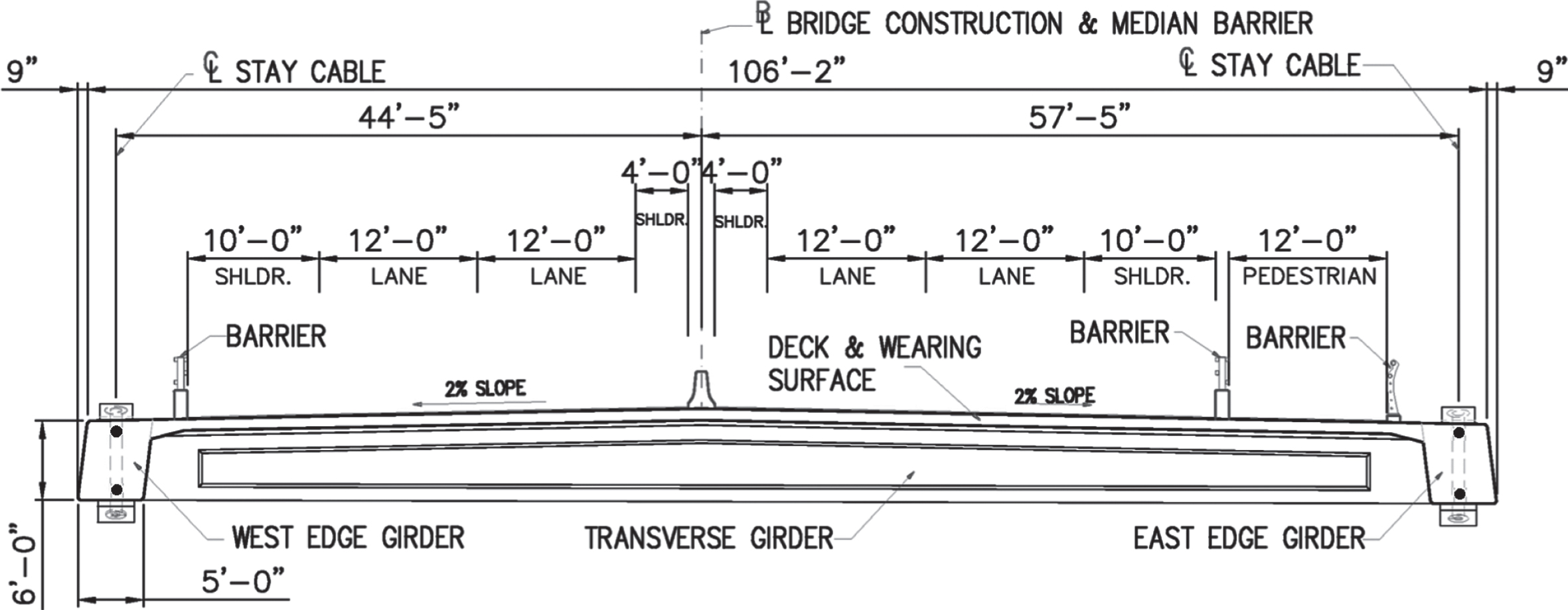
Bridge deck cross-section shown edge girders and sensor layout (indicated by black circles).

The bridge pylons are positioned well away from the inlet, which was a design requirement so that the inlet could be widened in the future if needed. As a result, both back spans and a major portion of the main span were constructed on falsework. A form traveler and cast-in-place construction was utilized on the main span over the inlet; precast and cast in-place construction were adopted for the back spans. Except for the middle 47.5 m (156 ft) of the main span, the minimum design strength of concrete for the edge girders and deck was 45 Mpa (6.5 ksi). The middle 47.5 m (156 ft) had a minimum design compressive strength of 48.3 MPa (7.0 ksi),

As just mentioned, construction of the bridge spanned over more than two years. The sequence of construction of the edge girders, transverse floor beams, and deck, and the different methods of construction, meant that the girders/deck were constructed over a period of many months, and with many individual concrete batches. As is well known, concrete strength can vary from batch to batch. It is dependent on the water content of the mix and the curing conditions. For a pour that lasts many hours, and in the case of the IRIB sometimes the better part of a day, the water content of the mix, the temperature, and the humidity could all vary, leading to varying concrete strength. Concrete cylinder break tests for the IRIB edge girders/deck, conducted over a period of 19 months, showed large variability in the compressive strength along the length of the bridge; the 56-day average strength was 57.7 MPa (8.4 ksi), while the minimum and maximum were 37.9 MPa (5.5 ksi) and 97.9 MPa (14.2 ksi), respectively (these are based on 110-cylinder breaks). A histogram of the measured concrete strength is shown in Fig. 3. Because of the type and sequencing of construction the edge girders and deck were not cast in sequence from one end of the bridge to the other, or from the abutments to the center. Casting lengths ranged from 7.3 m (24 ft) for construction with the form traveler to 22.0 m (72 ft) for construction on falsework. Furthermore, over the inlet both edge girders and the deck were cast together, while the east and west edge girders and deck that were constructed on falsework were all cast separately. All of these factors combined would suggest that, while exceeding the required minimum design strength, the strength, and therefore stiffness of the edge girders could vary along the length of the bridge, and from east to west edge girder.

Fig. 3

Histogram of edge girder concrete compressive strength based on 110 cylinder tests.

3 Structural health monitoring system

Because of its importance to the economy and tourism in the mid-Atlantic region and the fact that it is a signature structure, a structural health monitoring (SHM) system was installed on the IRIB bridge during construction. The concept was embraced by the owner and also by the Federal Highway Administration (FHWA); the FHWA provided a majority of the funds for the design and installation of the system, as part of the design-build project.

The design-build nature of the bridge construction meant that the SHM system would also follow a design-build approach. In the end a fiber-optic based system was adopted that includes numerous sensors, some of which are embedded in the concrete and others that are surface mounted. The suite of 135 fiber optic sensors includes accelerometers, strain, tilt, temperature, and displacement sensors. Data is collected 24 hours a day, 7 days a week at two different sample rates, a lower speed that captures slowly varying changes, and a higher speed that captures vehicles as they cross the bridge. The key sensors, for the purpose of this paper, are strain sensors embedded in the longitudinal edge girders. At 11 locations along the bridge are four strain sensors, two in each edge girder. One sensor is located near the top of the cross-section and one is located near the bottom of the cross-section, from which primary bending and axial force can be measured. Presented in Figs. 1 and 2 are the locations of the sensors along the bridge and within the cross-section. More information on the IRIB and structural health monitoring system can be found in [28].

4 Controlled load tests

A series of seven controlled load tests have been conducted on the bridge with the SHM system since it opened to traffic: the first in May of 2012, and then at the intervals, six months, one year, two years, four years, six years, and ten years. The load tests are part of an on-going program to monitor the bridge using the SHM system, not only for normal traffic and environmental loads, but also under very controlled load conditions. In the tests six heavily loaded 3-axle, 10-wheel dump trucks were utilized. The masses (weights) of the trucks at the six-month mark (Load Test 2) were very consistent: 28.3, 28.6, 27.8, 28.3, 28.4, and 28.3 Mg (62.5, 63.1, 61.2, 62.4, 62.7, and 62.4 kips). All six trucks had nearly identical axle spacings: 4.42 m (14 ft 6 in) front axle to first rear axle, and 1.4 m (4 ft 7 in) second to third axle. The tests are conducted at night and the bridge is closed to traffic as the test vehicles make slow speed “passes” (8–16 km/hr (5–10 miles/hr)) in various configurations across the bridge. As one might expect, because it is a new bridge, no significant variations in the strains recorded during the various tests have been observed to date. More details of the results and a comparison of the data from the different load tests can be found in [29].

The four-truck side-by-side pass completed during Load Test 2 (conducted in November of 2022) was used extensively for model calibration in this work. Figure 4 shows a plan view schematic of the four- truck configuration. Strain data was collected at 125 samples-per-second during the test.

Fig. 4

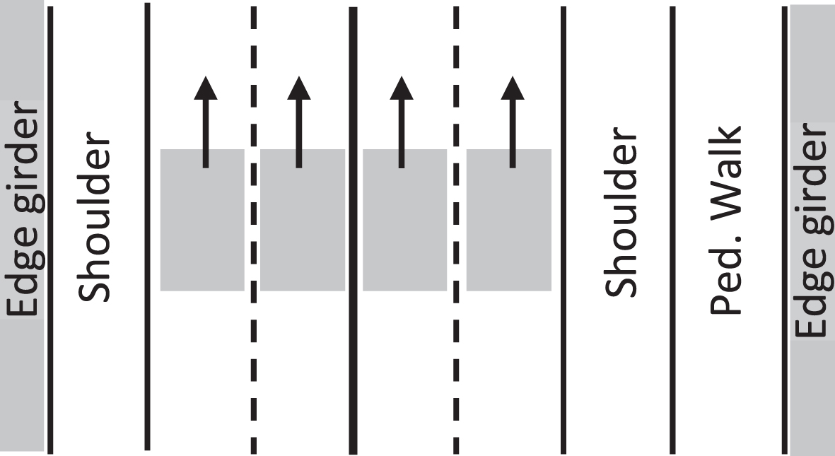
4-trucks side-by-side.

4.1 Data processing

A few steps were involved in post-processing the load test data to prepare it for use in model calibration. Presented in Fig. 5 is an example strain time history from an edge girder bottom strain sensor at midspan during the 4 side-by-side truck load pass (Fig. 4) which shows the raw data and the data after post-processing. Subtracting the initial baseline reading when there are no vehicles on the bridge from the record, “zeroed” the time history, thereby eliminating any offset in the measurement due to daily or seasonal temperature variations or other time-dependent factors. Next, a 200 point (1.6 sec) moving average was applied to the record to eliminate some of the underlying noise in the data. The 1.6 second moving average was found to be sufficient to eliminate the ambient vibration and signal noise of the recordings, and not suppress the peak strain measurement for these pseudo static measurements.

Fig. 5

Sample time history showing raw strain (in blue) and zeroed and smoothed strain (in red).

Strains were then extracted from the records at the instance when the vehicles produced their maximum effect at a given longitudinal sensor location. Referring to Fig. 6, which shows the sensor locations and the nine load positions used in the model calibration, this yielded nine load-case/strain data sets that were used for model calibration. As an example, when the load is at mid-span (position 3), which produced the peak strains in the east and west sensor #3 for the load pass, the strains from all sensors were extracted at the same time from the time histories.

Fig. 6

IRIB model with sensors and load case locations (each load represents 4 concentrated forces, spaced transversely, one for each truck in each travel lane).

Only the bottom edge girder sensors were used for the model calibration as these recorded the highest strain readings. Not including the sensors at the pylons (Fig. 1) and the top edge girder sensors, this yielded nine longitudinal sensor positions with two sensor measurements each for a total of 18 sensors, and nine longitudinal vehicle positions, for a total of 18×9 = 162 measurements per truck pass. The final step was to eliminate any strain measurement that was less than 2.5μɛ that is the lower threshold used to eliminate small measurements that are prone to error and any remaining system noise. This yielded 110 strain measurements and 9 load positions to be used in the model calibration. The strains are listed in the appendix.

5 Darwin calibration tool

A generic formulation and software tool have been developed by the fourth author and a team at Bentley Systems, Inc. for finite element model calibration that is integrated with STAAD Pro [30]. The integrated approach allows engineers to calibrate a FE model with sensor responses that include displacements, strains, frequencies, and mode shapes. The calibration is carried out by adjusting the material and/or geometry attributes for the groups of aggregated elements to minimize the error function E_T or the objective function, which is defined as the difference between monitored and analysed responses including mode shapes, frequencies, displacements and strains. The objective function/fitness value is given as [31]: $\begin{matrix} FV = E_{m} (∥ φ_{i}^{M} - φ_{i}^{A} ∥) + E_{f} (∥ f_{i}^{M} - f_{i}^{A} ∥) \\ + E_{d} (∥ d_{j}^{M} - d_{j}^{A} ∥) + E_{ɛ} (∥ ɛ_{k}^{M} - ɛ_{k}^{A} ∥) \end{matrix}$ (1) where $φ_{i}^{M}$ and $φ_{i}^{A}$ are the monitored and analysed modal shapes respectively, $f_{i}^{M}$ and $f_{i}^{A}$ are the monitored and analysed modal frequencies, $d_{j}^{M}$ and $d_{j}^{A}$ are the monitored and analysed displacements, $ɛ_{k}^{M}$ and $ɛ_{k}^{A}$ are the monitored and analysed strains respectively, E_m, E_f, E_d, and E_ɛ are the error functions of mode shapes, frequencies, displacements and strains, respectively. Each of the error functions can take the form of Mean Absolute Percentage Error (MAPE), Absolute Sum (AbsSum), or Root Mean Square Error (RMSE).

The finite element model calibration is an implicit nonlinear optimization problem, which is solved by using the Darwin Optimization Framework tool [31 –33]. The integrated model calibration software is a proprietary tool that is not open source or commercially available but can be made available to third parties under agreement with Bentley Systems, Incorporated. It uses a fast messy generic algorithm [34] and features of parallel computation by using a many-core personal computer or a network of machines. The user is able to choose from the multiple objective functions in (1) to search for the near optimal solution. The input data for model calibration can be strains or displacements, in conjunction with static load cases, or frequencies and mode shapes, in conjunction with dynamic excitations. The user can choose to optimize section properties, material properties, boundary conditions, or combinations thereof. It is noted that multi objective optimization is only recommended if the error functions are in conflict each other, such as paring modal shapes for model calibration or damage detection [35]. When local response such as strain response is employed for model calibration, it is highly unlikely that minimizing the error for one strain sensor will be in conflict with other others. Therefore, single objective optimization is adequate.

In this work the edge girder bottom sensor strain data was used to calibrate the elastic modulus of the girders. Elastic modulus is related to concrete strength through the generally accepted equation $E_{c} = 4700 \sqrt{f_{c}^{'}}$ (2) in which E_c is concrete modulus in MPa and $f_{c}^{'}$ is concrete compressive strength in MPa. Using the calibrated elastic modulus of the edge girders ${\tilde{E}}_{c}$ the concrete strength ( ${\tilde{f}}_{c}^{'}$ ) corresponding to the calibrated modulus can be calculated as ${\tilde{f}}_{c}^{'} = {({\tilde{E}}_{c} / 4700)}^{2}$ (3) and correlated to the measured concrete strength given in Fig. 3.

6 IRIB model calibration

The objective of the calibration was to determine the best model for predicting the live load response of the bridge due to heavy vehicles, through calibration of the main longitudinal load carrying member, i.e., the girders and deck. Strain data was not collected during the staged construction of the bridge and therefore the model could not be calibrated for dead load. However, in conjunction with dead load stresses determined from the design, the calibrated model can be used for load rating and permit vehicle evaluation going forward. In addition, once calibrated, the effects of creep and shrinkage, aging, and deterioration can be assessed by comparing the output results obtained now, to those obtained from a calibration conducted using similar load tests conducted in the future. Future work may investigate calibration of the bridge bearings based on their displacements due to temperature changes, but which are too small under vehicle loads to be used for calibration.

6.1 Description of the model

A STAAD.Pro model of the IRIB was developed with 771 elements and 470 nodes (Fig. 7). The edge girders, transverse floor beams, and pylons were modeled with three dimensional bending elements that have six degrees of freedom at each end. The stay cables were modeled as two-force members that can carry tension or compression (i.e., a decrease in the assumed dead load force in the stay).

Fig. 7

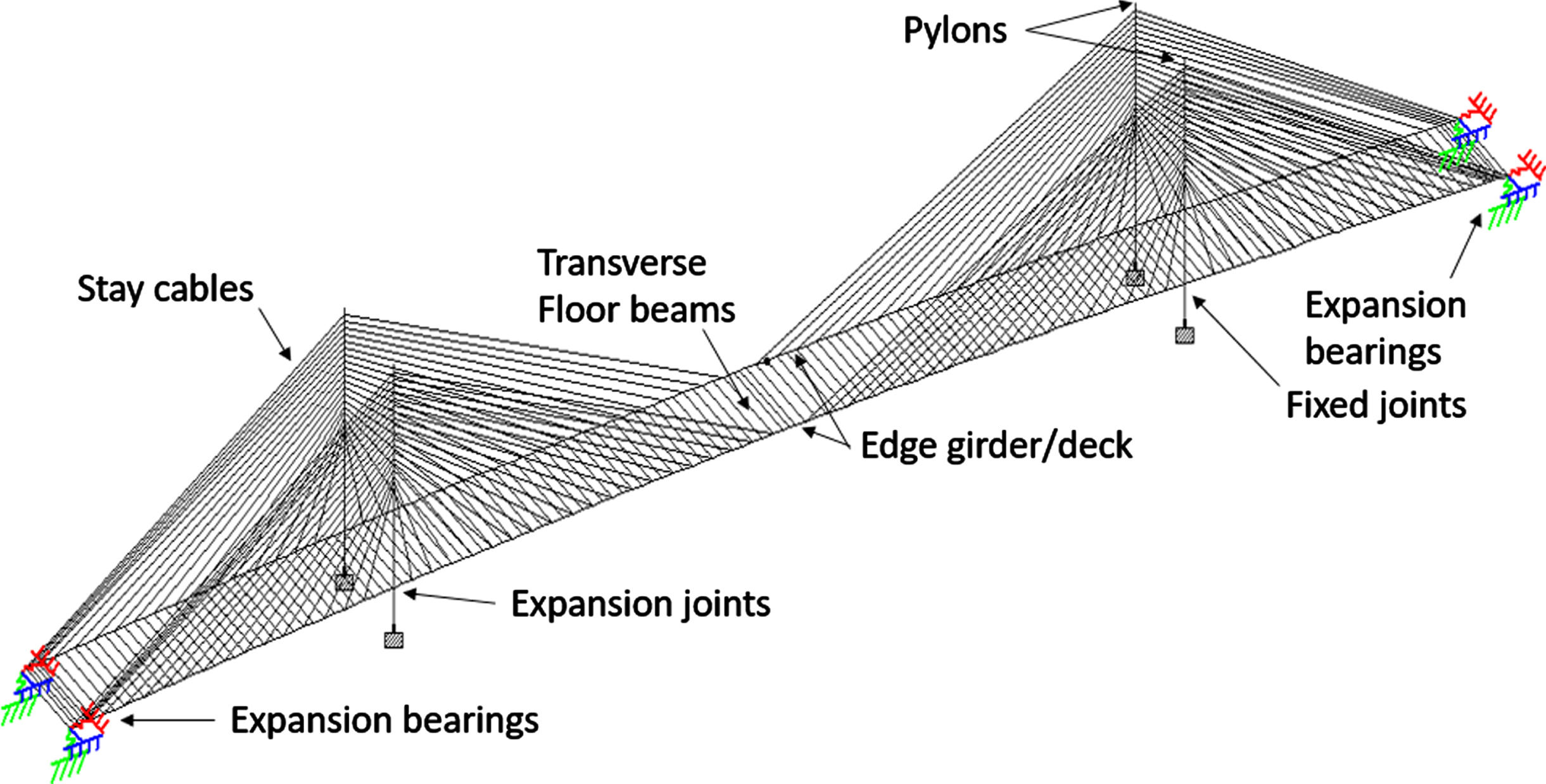
IRIB finite element model.

The deck-to-pylon bearings are fixed at the north pylon, and free to expand and rotate at the south pylon and both abutments. Based on the details of the bearings and restraints, at the north pylon the relative displacements between the deck and pylon were restrained in all directions and moments were released in all directions. At the south pylon the relative displacements between the deck and the pylon in the vertical and transverse directions were restrained, and a linear spring allowed relative movement in the longitudinal direction, the stiffness of which was calculated based on the design of the elastomeric bearing; moments were released in all directions. At the abutments displacements were restrained in the transverse direction, and displacements and rotations in all other degrees of freedom were modeled as elastic supports with stiffnesses calculated based on the design of the bearings at these locations.

The edge girder elements were modeled to represent the edge girder and the effective width portion of the deck: the moment of inertia of the edge girder/deck members was equal to the design value of 1.672 m⁴ (193.2 ft⁴). This was based on the gross properties of the cross section, including the overlay, and an effective deck width of 7.63 m (25 ft) that was used in the design. The gross property assumption was based on the design requirement of no cracking of the concrete.

The compressive strength of the edge girders of the design, i.e., initial uncalibrated model, mimics the design strength: 45 MPa (6,500 psi) along the length of the bridge with the center 47.5 m (156 ft) having a compressive strength of 48.3 MPa (7,000 psi). The compressive strength of the pylons was equal to 45 MPa (6,500 psi).

Figure 6 shows the location of the 18 strain sensors, all of which are measured at the bottom of the edge girder. The nine load cases are also shown in Fig. 6. Each load case is represented by four point loads spaced transversely across the deck according to the four travel lanes to represent four trucks (for clarity in the figure the loads are shown as single concentrated forces in Fig. 6).

6.2 Calibration

The objective of the calibration was to determine the optimal distribution of the modulus of elasticity of the longitudinal edge girders, along the length of the edge girders, that would yield the best prediction of the measured strains. The east and west edge girders were modeled with 180 beam elements each; however, to calibrate the model the edge girder elements were aggregated into groups to form regions of equal modulus of elasticity, with the modulus of each group representing one calibration parameter. For example, in the 6 parameter model (Fig. 8(a)) the south back span elements of the west girder were aggregated to form one parameter, the main span elements of the west girder formed a second parameter, and the north back span elements formed a third group. The process was repeated for the east girder to yield a total of 6 parameters. Other models were created by grouping edge girder elements to form 10, 14, and 18 parameter models. In all cases the element grouping was identical for the east and west edge girder. All four models are shown in Fig. 8; the element group breakdown by span is shown in Table 1. The element groups were dictated by the locations of the strain sensors in the edge girders (each element group would have at least one strain measurement within its region). It is these element groups that are calibrated in the models. The calibration results of these models were then compared to determine the influence of parameter grouping.

Fig. 8

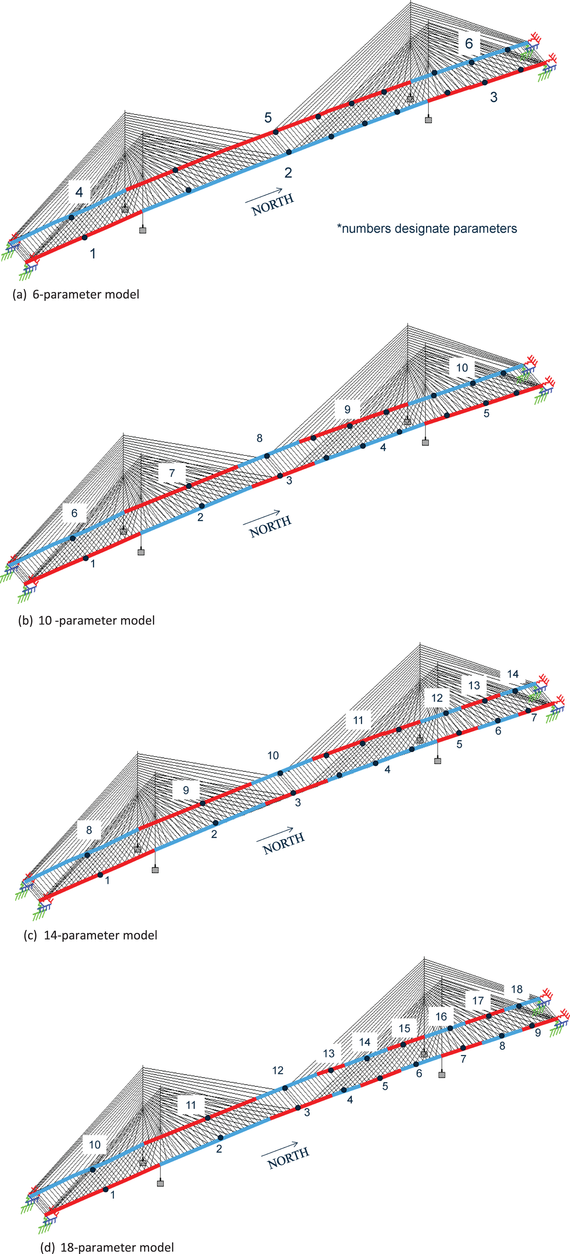
Calibration models (calibration element groups numbered and shown alternately in blue and red) (a) 6-parameter model, (b) 10-parameter model, (c) 14-parameter model, (d) 18-parameter model.

Table 1

Calibration models – element groups

No. model calibration parameter groups	No. element groups per edge girder	No. element groups south back span	No. element groups center span	No. element groups north back span
6	3	2	2	2
10	4	2	6	2
14	7	2	6	6
18	9	1	5	3

The GA calibration tool generates the initial population of solutions in a random process and searches the entire user specified solution space for the near-optimal solution by emulating Darwin’s natural selection principle survival of the fittest and genetic reproduction. It requires a random seed value between 0 and 1 to generate the initial population within the defined solution space. Because of the stochastic nature of the GA process, one would expect similar results even when using different seed values. To confirm this, three calibration runs were conducted for each model, each with a different seed value (0.2, 0.5, and 0.7). The average solutions of the three runs are used as the calibrated parameters for the model.

The objective function/fitness value used for the calibration is a weighted Root-Mean-Square Error between the measured strains and the calculated peak strains, as given by E_ɛ in Equation (1), i.e. [31], $FV = E_{ɛ} = \sqrt{\frac{1}{\sum_{k = 1}^{n} w_{i}} \sum_{k = 1}^{n} w_{i} {(ɛ_{k}^{M} - ɛ_{k}^{A})}^{2}}$ (4) in which FV is the fitness value, $ɛ_{k}^{M}$ and $ɛ_{k}^{A}$ are the measured and calculated strains, respectively, w_i are the weighting factors, and n = 110 is the total number of strain measurements. The weights were equal to 1 for all strains except the maximum strain in the east and west girder for a given load case, which were set equal to 2. This placed greater emphasis on matching the highest strains for a given load position.

Before moving to the results of the calibrations it is useful to examine the fitness of the original, uncalibrated design model. The strain values calculated using the design (initial) model are compared to the measured load test strains in Fig. 9. Shown by the bar chart in the figure and the left y-axis is a maximum strain envelope for the sensors in each of the nine load cases (each sensor reaches its maximum value for loads in a different location). The line graph (right y-axis) indicates the percent difference between the calculated and measured strains. Most of the percent differences of the design model compared to the measured response are greater than 10%, with the largest difference being 42%. The difference is less than 10% for only six out of 18 sensor locations. The design model is in reasonable agreement with the test results, but clearly improvements can be made, which is the goal of the model calibration.

Fig. 9

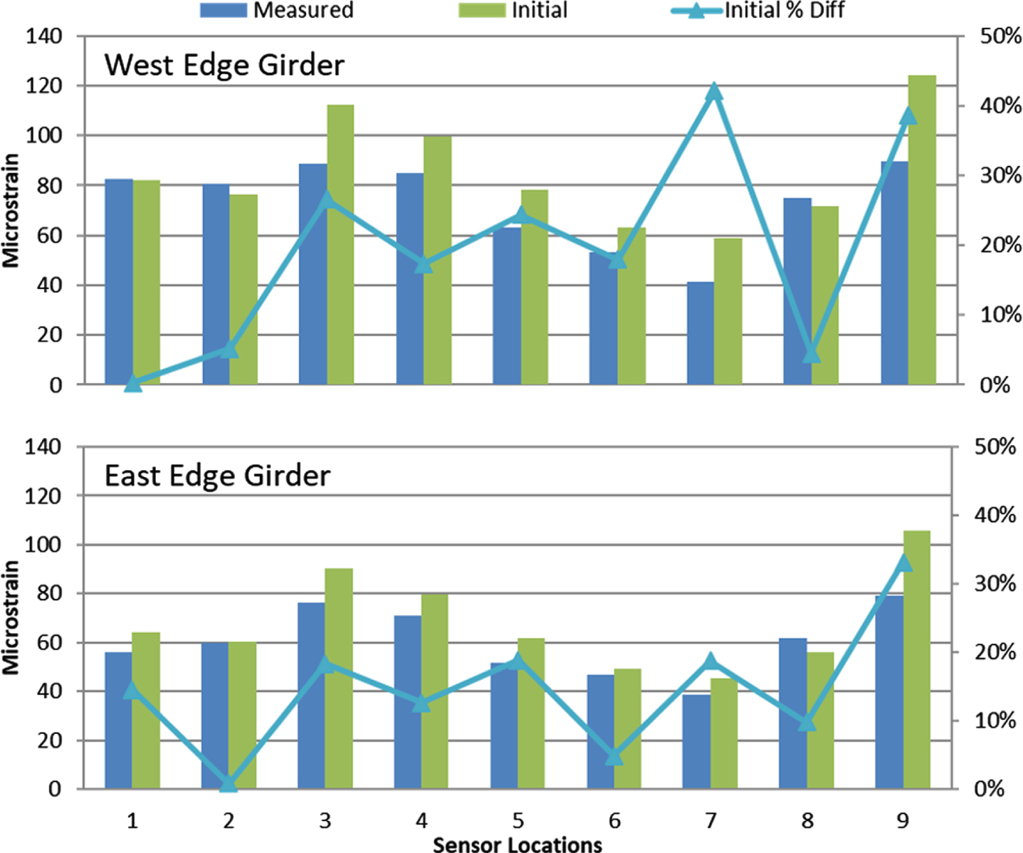
IRIB design model compared to measured load test results.

6.3 Calibration results

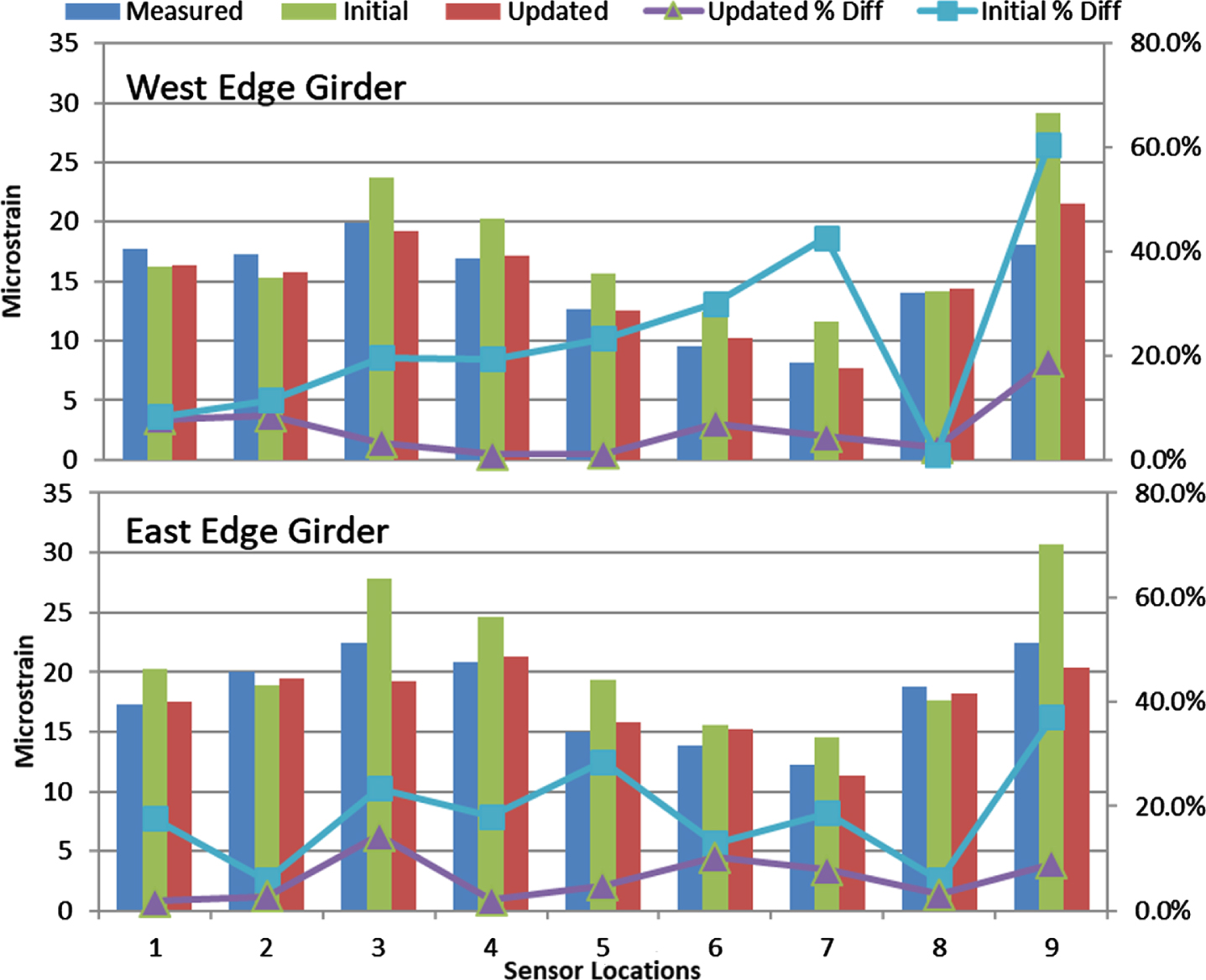
Calibrations were first performed using six parameters (6 element groups), with each span containing one parameter for the east and west edge girders (Fig. 8 (a)). The results of the 6-parameter calibrations are shown in Fig. 10. The strain values for the measured (target) response, the design model, and the calibrated model are compared, along with the percent difference of the measured response to the design and calibrated models. The calibrated model better represents the measured data than the design model with most of the results improving as a result of the calibration. The maximum error in the calibrated model is 24% in the east girder at sensor #8. The error is less than 10% for 13 of 18 locations, and less than 5% for 10 of 18 locations.

Fig. 10

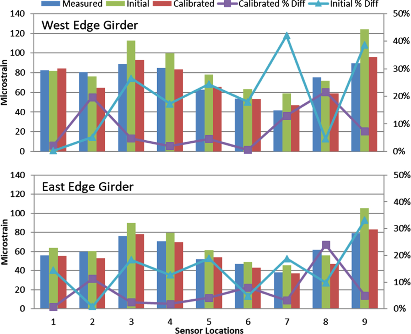
6-parameter calibration results.

Another way to view the results is by comparing the back calculated concrete compressive strength based on the calibrated modulus (Equation 3) to the measured average strength. A weighted average compressive strength has been calculated based on the calibrated elastic modulii (Equation 3) and the corresponding length of each parameter. For the 6-parameter model the weighted average compressive strength is 72.7 MPa (10.5 ksi), which is 26% higher than the measured strength (57.7 MPa (8.4 ksi)). Note that the design strength, which would likely be used in an uncalibrated model for load rating and analysis of the bridge, is 22% lower than the measured strength.

The 18-parameter group model is shown in Fig. 8(d). The 18 groups are based on the location of the 18 strain sensors: the south span girders have one parameter each, the main-span girders are split into five parameters each based on the strain sensor locations in the span, and the north span girders are split into three equally spaced parameters. The results of the 18-parameter calibrations are shown in Fig. 11. The error is less than 10% for 16 out of 18 of the locations, and less than 5% for 12 of the 18 measurements; the maximum difference is 18%. The weighted average concrete strength is 72.9 MPa (10.6 ksi) which is 26% higher than the measured average 56-day compressive strength.

Fig. 11

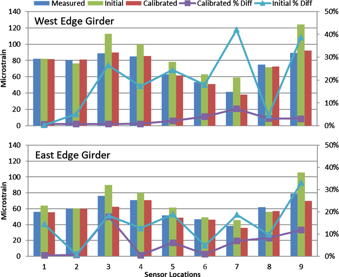
18-parameter calibration results.

Calibrations were also performed with 10 and 14-parameter groups. For 10-parameters (Fig. 8(b)), the main-span was split into thirds while the parameters in the north and south span were similar to the 6 parameter model. These results show improvement over the 6-parameter calibrations. The 10-parameter calibration is a more accurate calibration than the 6-parameter calibrations, with the greatest percent difference being 22.2%. The error is less than 10% for 15 out of 18 of the locations, and less than 5% for 11 of the 18 measurements. The weighted average compressive strength of the 10-parameter model is 67.2 MPa (9.75 ksi), 16% higher than the measured average 56-day compressive strength.

The 14-parameter group boundaries are set by keeping the south span as one parameter on the east and west, the main-span was split into three parameters, and the north span was split into three equally spaced parameters (Fig. 8(c)). The 14-parameter calibration is the best representation of the measured response data: it is better than the 6 and 10 parameter models by several measures, and marginally better than the 18-parameter model. The error is less than 10% for 18 out of 18 of the locations, and less than 5% for 14 of the 18 measurements; the maximum difference is 9.0%. The weighted average compressive strength is 72.0 MPa (10.4 ksi), which is 25% higher than the measured average 56-day compressive strength.

The results of the calibrations with different parameter groups are shown in Table 2. The fitness value quantifies the goodness-of-fit and is calculated using Equation (4). The design model had a fitness value of 9.48 microstrain. The fitness values for each parameter grouping shown in Table 2 are the average of the three calibration runs with the different seed values. The fitness value from the best calibration out of the three runs is also shown: the best calibration is the one with the lowest fitness value. Comparing the average to the best fitness shows that there was good consistency in the results. The percent improvement is calculated by the difference between the design model’s fitness value and the average fitness value. The percent improvement increases as the number of parameter groups increases from 6, to 10, to 14 parameters, and then decreases slightly for the 18 parameter model, but the 18 parameter model is still better than the 10 parameter model. The slight decrease in performance of the 18 parameter model compared to the 14 parameter model is because there is only one sensor measurement within each element group of the 18 parameter model, whereas the 14 parameter model has some element groups that have multiple sensor measurements within the group domain.

Table 2

Summary of fitness results

Model	Ave. Fitness Value	Best Fitness Value	% improvement rel. to design/initial
Design/Initial	9.48	–	–
6	5.84	5.82	38%
10	5.33	5.31	44%
14	4.70	4.66	50%
18	5.10	5.08	46%

A summary of the results from the different parameter calibrations are shown in Fig. 12. Calibrations with 6- and 10-parameters show similar results. The calibration did not improve the model’s ability to match all of the strain sensors when there were parameter groups that contained more than one strain sensor. For example, the 6-parameter set (Fig. 8) contains multiple sensors in the main-span and north span parameters, which means that the calibrated elastic modulus must be a constant along the length of the span; this does not allow it to match the response of every strain sensor. The 14-parameter and 18-parameter model results were very similar, with the 14-parameter model yielding slightly better agreement; both showed favorable improvement over the initial design model.

Fig. 12

Summary of parameter results.

Two other calibration models were tested with other parameter groupings. An 18- parameter model was created with the groupings symmetrically distributed on the bridge, i.e., with three equal groups per span, per girder. In this case, noting again the sensor layout in Fig. 6, there were four parameter groups that did not have a sensor within their domain. Another model was created with a very large number of parameters, 57 in total, which was guided by the edge girder casting sequence during construction, i.e., each group represented an actual casting segment on the bridge. In both cases the calibration results were not as good as the 14 or 18 parameter results presented earlier. It was found that the estimated modulus for parameters that did not have a sensor within their domain were grossly in error. This can be explained by the fact that strain is a very localized behavior, and without a target strain within the parameter domain, the modulus is free to diverge significantly without affecting the neighboring parameter estimations. Should displacements or some other global measure be used for calibration it is expected that this would not be the case.

6.4 Sensitivity analysis – effect of measurement noise

For the strain data collected during a controlled load test the noise and variability effects can be divided into two categories: variability due to slight variations in the execution of replicate truck passes, and errors/noise due to the sensor and SHM system. Data was collected with the monitoring system to quantify these factors and then used to randomly perturb the peak strains from the load test in repeated calibrations, to assess the effect of the measurement noise on the calibration results.

During the load test the side-by-side truck passes are made at a crawl speed and the drivers of the vehicles, while being very careful, rarely form a perfect straight line, as depicted in Fig. 4. Therefore, even for similar passes there are slight variations in the peak strains recorded by a sensor due to the longitudinal and transverse positions of the vehicles relative to each other. To assess this variability multiple passes of the same type were made in Load Test 4. The strain time histories were processed as described previously (zeroing and smoothing) and the variability of the reduced peak strain data was calculated. The standard deviation of the peak strains for the replicate passes was 0.56μɛ. To assess the system noise, data was recorded for several minutes at night when there was no traffic on the bridge and little to no wind and post-processed as described for the truck passes (zeroing and smoothing). The standard deviation of the system noise after processing was 0.74μɛ. The combined root-mean-square value of these effects were calculated and are equal to $σ = \sqrt{{(0.56)}^{2} + {(0.74)}^{2}} = 0.93 μ ɛ$ . Assuming these effects are normally distributed the peak strain measurements have a range of error of ±2.8μɛ.

Using the 14-parameter model the effect of the noise on the calibration results was investigated by adding artificial noise to the measured strains from Load Test 2 (Appendix) and comparing the results with those obtained without the artificial noise. To do this simulated measurement noise was generated from a zero-mean normal distribution with a standard deviation of 0.93μɛ and added to the strain of a sensor for a given load case. Thus, every strain measurement was perturbed by a unique strain within the range $- 2.8 μ ɛ \leq \tilde{ɛ} \leq + 2.8 μ ɛ$ of the measured value. Ten calibrations were run for each load case reported, each using a unique set of perturbations.

Fitness values ranged from 4.77 to 5.04, with the average being 4.89μɛ. The coefficient of variation of the 14 calibration factors ranged from 0 to 5.8%, with the average being 3.2%. The results show that the calibration is relatively insensitive to measurement error inherent in the SHM data.

6.2 Effect of traffic barriers

The flexural stiffness of the edge girders is proportional to EI, where E is the modulus of elasticity and I is the moment of inertia. For a concrete bridge with an integral edge girder/deck cross-section, such as the IRIB, an assumption must be made about the effective width of the cross section that is used in calculating the moment of inertia. AASHTO [36] provides guidance on how to estimate the effective width [36], which for the design was 7.63 m (25 ft) along the majority of the bridge, and 9.15 m (30 ft) for the middle 91.5 m (300 ft) of the main-span. The moment of inertia corresponding to this effective width is, 1.672 m⁴ (193.2 ft⁴) and 1.805 m⁴ (208.6 ft⁴), respectively, per the design calculations. The actual effective width is likely something other than these values, because of the contribution of the traffic and pedestrian barriers on the bridge (see Fig. 2). It likely also varies along the length of the bridge, to a greater extent than the simply assumed two values. If the moment of inertia of the cross-section in the model is changed, the calibrated modulus of elasticity would be affected, with the product of the two being the same for any calculation. This was confirmed with several calibration runs.

For all of the calibrations discussed thus far, the moment of inertia of the edge girders was constant and equal to 1.672 m⁴ (193.2 ft⁴) over the entire span, except for the middle 91.5 m (300 ft) of the main span which has a moment of inertia to 1.805 m⁴ (208.6 ft⁴). Again, these values were the moments of inertia used by the designer. With the addition of the 0.61 m by 0.30 m (2-foot by 1-foot) jersey barrier to the edge girder geometry, the moment of inertia of the section, assuming a 7.63 m (25 ft) effective width, increases to 1.851 m⁴ (213.9 ft⁴). For an effective width of 9.15 m (30 ft) and including the jersey barrier, the moment of inertia increases to 1.969 m⁴ (227.5 ft⁴).

Using these values and proportioning the calibration results obtained with the original design moment of inertia, yields adjusted average concrete strengths that are very close to the measured average strength. Table 3 summarizes the back calculated weighted average concrete strength for the models without the traffic barrier and for the models with the traffic barrier and lists the percent difference relative to the measured strength. One can see that the average strength for the models with the traffic barrier included are very close to the measured strength, with all of the calibrated strengths being within 4.5% of the measured value.

Table 3
Weighted average concrete strength of calibrated models and % difference relative to the measured average strength (57.7 MPa)

Model No traffic barrier With traffic barrier

(# parameters) Ave Strength (MPa) % Diff Ave Strength (MPa) % Diff

6 72.7 26 59.7 3.4

10 67.2 16 55.1 –4.5

14 72.0 25 59.2 2.5

18 72.9 26 59.8 3.7

Model	No traffic barrier	With traffic barrier
6	72.7	26	59.7	3.4
10	67.2	16	55.1	–4.5
14	72.0	25	59.2	2.5
18	72.9	26	59.8	3.7

7 Model validation

During the controlled load test #2, conducted in November of 2012, a total of 23 different load passes were conducted using various configurations of six similar, and similarly loaded, ten wheeled dump trucks. Only one of those load passes was used to calibrate the model – that is a four truck side-by-side load pass as shown in Fig. 4. Note that this load pass is symmetric with respect to the travel lanes, but is shifted west relative to the center of the bridge due to the pedestrian walkway. To validate it, the calibrated model was used to compute the strains for four other truck passes that were not used in the calibration. Results were compared for data recorded during a six truck, side-by-side load pass (a heavier combined load than was used for model calibration), and three one truck load passes (lighter loads, and loads that are further offset from the centerline of the bridge than the four truck load that was used for model calibration) (Fig. 13). For this work the calibrated 18 parameter model was used.

Fig. 13

Truck passes used for model validation.

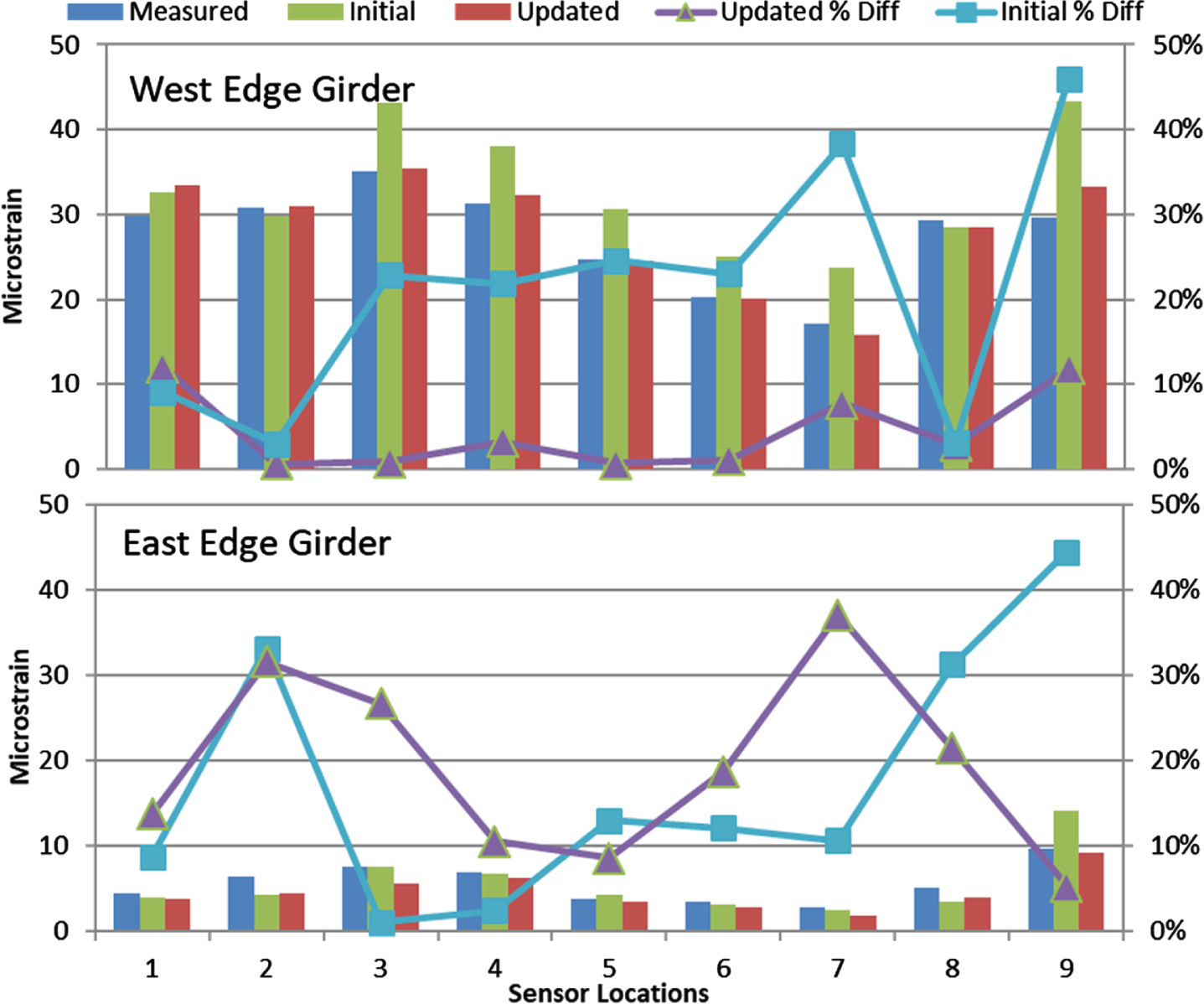
The results of the validations are shown in Figs. 14 to 17. The figures show that the model’s strain response matches various different loading configurations with similar precision as it matches the load pass that the model was calibrated with. Slightly larger percent differences in the calibrated strains in the girder opposite the truck are observed for the 1-truck passes in the shoulder, in particular for the east girder of the southbound 1 truck shoulder pass (Fig. 17). This can be explained by the very low strains that develop in the opposite side for the light one truck load. The results show, however, that good agreement was obtained for a heavier load, lighter loads, and loads that were further offset from the centerline of the bridge, thus validating the calibrated model’s ability to accurately predict the bridge response to live vehicle loads.

Fig. 14

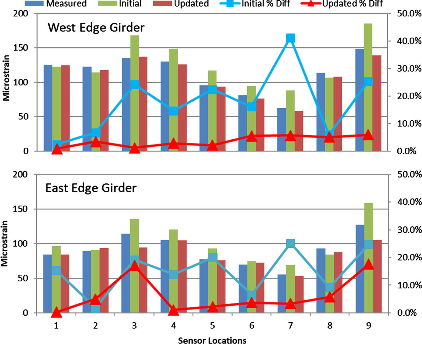
6-truck validation results.

Fig. 15

1-truck northbound fast-lane validation results.

Fig. 16

1-truck northbound shoulder validation results.

Fig. 17

1-truck southbound shoulder validation results.

8 Conclusions

A detailed model of the Indian River Inlet Bridge in Delaware was developed and calibrated, using strain data from controlled load tests of the bridge that were recorded using the permanent SHM system on the bridge. The model was calibrated using Bentley Systems, Inc.’s DarwinSHM Calibration tool [37, 38]. The modulus of elasticity of the main longitudinal load carrying members of the bridge, the edge girders, were calibrated based on a four truck, side-by-side load pass. Calibrations were performed using 6, 10, 14, and 18 aggregated beam groupings, i.e., calibration parameters. The effects of measurement noise on the results were established and the results were then verified using multiple, independent truck passes. Based on these results the following conclusions can be stated:

Calibration produced a model that better predicts the behavior of the as-built structure, as compared to the design model. The 14 and 18- parameter models yielded the best results, with errors less than 10% for the majority of sensor measurements. Models with 6 and 10 parameters showed improvement over the design model but were not as effective as the models with more parameters.

The results of concrete cylinder tests from when the bridge was constructed showed tremendous variability, which would manifest itself as spatial variability in the flexural stiffness of the edge girders. The calibration procedure was able to capture that variability, resulting in significantly better agreement between the live load measured strains and the model predicted strains. While the results presented here are specific to the Indian River Inlet bridge, they do show the importance and need for considering the variability of concrete in general in large cable stayed bridges in order to more accurately predict the true behavior of the structure. The approach could be extended to calibration of the concrete pylons as well, provided sufficient strain data is available from the pylons.

Using the design moments of inertia, the weighted average compressive strength of the edge girder concrete obtained with the calibrated model is approximately 25% higher than the average measured strength. When the traffic and pedestrian barriers are included, the weighted average compressive strength is no more than 4% higher than the measured average strength for the 14 and 18 parameter models.

The calibration was shown to be insensitive to the inherent measurement noise of the SHM data.

The model was validated with multiple independent truck passes.

When partitioning parameter groups to be calibrated, the initial notion is to generate the maximum number of logical groupings based on known design parameters or construction sequences. For the IRIB, this would require 57 parameters to correspond to the concrete pours of the edge girders and deck during construction. However, through calibrations with different parameter grouping sets it was noted that parameters that did not contain a response value (strain sensor) within its boundaries were unable to be calibrated with any level of precision. With this conclusion, the maximum number of parameter groups would be determined by the number of sensors within the regions being calibrated.

The calibrated model can be used by the owner to conduct load ratings of the bridge, evaluate permit vehicles, and to assess degradation in performance over time with recalibration using future load test results.

Footnotes

Acknowledgments

The authors would like to acknowledge the Delaware Department of Transportation for their continued and enthusiastic support of structural health monitoring of the IRIB, for their support in conducting the controlled load tests of the IRIB, and for partial financial support of the research. The University of Delaware authors would like to acknowledge and thank Bentley Systems Inc. for support of the graduate students who did the work and support in using the calibration tool.

Funding statement

Bentley Systems Inc. provided funding in the form of a graduate assistantship to support the first author.

Conflict of interest statement

The authors have no conflict of interest to report.

Author contributions

Natalicchio – performance of work, interpretation of data, writing the article, formal analysis, data curation, writing – original draft, visualization

Al-Khateeb – methodology

Chajes – writing (review and editing),

Wu – software, writing (review and editing)

Shenton – conceptualization, funding acquisition, supervision, project administration,

All authors had access to the data.

Appendix: Strain data (in microstrain) used in model calibration

Load Case	Sensor	East Girder	West Girder	Load Case	Sensor	East Girder	West Girder
	1	55.9	82.3		2	–3.2	–4.2
	2	–10.9	–11.0		3	–3.7	–5.0
1	3	–3.8	–4.6	5	4	6.9	7.3
	4	3.6	4.2		5	51.8	62.9
	7	–5.7	–3.8		6	–12.4	–15.6
	9	–6.1	–7.5		7	–4.5	–2.7
	1	–13.1	–20.3		8	–14.2	–16.1
	2	59.7	80.6		9	–23.4	–24.2
2	3	–4.1	–4.5		6	46.9	53.4
	4	–7.9	–8.0	6	7	–6.9	–4.7
	5	–3.3	–2.2		8	–9.9	–10.2
	9	–5.8	–7.9		9	–12.3	–13.3
	1	–8.8	–13.8		4	–5.4	–4.2
	2	–18.6	–22.6		5	–3.8	–2.8
	3	76.1	88.8	7	7	38.4	41.5
3	5	–16.3	–19.5		8	13.4	14.7
	6	–9.0	–10.8		9	6.1	4.8
	8	–10.0	–11.8		4	–8.0	–7.3
	9	–23.5	–25.9		5	–5.9	–4.4
	1	–2.6	–5.0	8	7	–6.7	–9.6
	2	–10.0	–11.4		8	62.0	75.0
	3	6.9	6.8		9	14.3	12.9
	4	70.9	84.8		3	–3.8	–3.8
4	5	–11.5	–15.1		4	–9.2	–8.2
	6	–18.1	–21.2		5	–5.7	–3.9
	8	–15.0	–17.4	9	7	–18.1	–20.2
	9	–31.1	–33.3		8	–3.5	–6.8
					9	79.3	89.4

References

Hart

, Yao

JT-P

. System identification in structural dynamics. Journal of the Engineering Mechnics Division. 1997;103(6):1089–104.

Mottershead

, Friswell

. Model updating in structural dynamics: A survey. Journal of Sound and Vibration. 1993;167(2):347–75.

Catbas

, Kijewski-Correa

, Aktan

. Structural identification of constructed systems: Approaches, methods, and technoligies for effective practices of St-Id, American Society of Civil Engineers, Reston, VA, 2013.

Ribeiro

, Calcada

, Delgado

, Brehm

, Zabel

. Finitel element model updating of a bowstring-arch railway bridge based on experimental modal parameters. Engineering Structures. 2012;40:413–35.

Jang

, Li

, Spencer

. Corrosion estimation of a historic truss bridge using model updating. Journal of Bridge Engineering. 2013;18(7):678–89.

Garcia-Palencia

, Santini-Bell

, Sipple

, Sanayei

. Structural model updating of an in-service bridge using dynamic data. Structural Control and Health Monitoring. 2015;22(1):1265–81.

Zhang

, Zhang

, Guo

, Xu

, Wu

. Structural identification of short/middle span bridges by rapid impact testing: Theory and verification. Smart Materials and Structures. 2015;24.

Dubbs

, Moon

. Assessment of long-span bridge performance issues through an iterative approach to ambient vibration-based structural identification. Journal of Performance of Constructed Facilities. 2016;30(5).

Whelan

, Zamudio

, Kemicky

. Structural identification of a tied arch bridge using parallel genetic algorithms and ambient vibration monitoring using a wireless sensor network. Journal of Civil Structural Health Monitoring. 2018;8:315–30.

10.

Schlune

, Plos

, Gylltoft

. Improved bridge evaluation through finite element model updating using static and dynamics measurements. Engineering Structures. 2009;31:1477–85.

11.

Deng

, Cai

. Bridge model updating using response surface method and genetic algorithm. Journal of Bridge Engineering. 2010;15(5):553–64.

12.

Hasancebi

, Dumlupinar

. Linear and nonlinear model updating ofreinforced concrete T-beam bridges using artificial neural networks. Computers and Structures. 2013;119:1–11.

13.

Zhou

, Prader

, Weidner

, Dubbs

, Moon

, Aktan

. Structural identification of a deteriorated reinforced concrete bridge. Journal of Bridge Engineering. 2012;17(5):774–87.

14.

Gokce

, Catbas

, Mustafa

, Frangopol

. Structural identification for performance prediction considering uncertainties: Case study of a movable bridge. Journal of Structural Engineering. 2013;139(10):1703–15.

15.

Jung

, Kim

. Finite element model updating on small-scale bridge model using the hybrid genetic algorithm. Structure and Infrastructure Engineering. 2013;9(5):481–95.

16.

Sanayei

, Khaloo

, Mustafa

, Catbas

. Automated finite element model updating of a scale bridge model using measured static and modal test data. Engineering Structures. 2015;102:66–79.

17.

Xiao

, Xu

, Zhu

. Multiscale modeling and model updating of a cable-stayed bridge II: Model updating using modal frequencies and influence lines. Journal of Bridge Engineering. 2015;20(10).

18.

Zhou

, Zhang

, Yi

, Jiang

, Pan

. Structural identification of a concrete-filled steel tubular arch bridge via ambient vibration test data. Journal of Bridge Engineering. 2017;22(8).

19.

Feng

, Feng

. Model updating of railway bridge using in situ-dynamic displacement measurement under trainloads. Journal of Bridge Engineering. 2015;20(12).

20.

Khuc

, Catbas

. Structural identification using computer vision-based bridge health monitoring. Journal of Structuaral Engineering. 2018;144(2).

21.

Yarnold

, Moon

, Aktan

. Temperature-based structural identification of long-span bridges. Journal of Structural Engineering. 2015;141(11).

22.

Murphy

, Yarnold

. Temperature-driven structural identification of a steel girder bridge with an integral abutment. Engineering Structures. 2018;155.

23.

Perterson

, Oiseth

. Sensitivity-based finite element model updating of a pontoon bridge. Engineering Structures. 2017;150:573–84.

24.

Zhu

, Xu

, Xiao

. Multiscale modeling and model updating of a cable-stayed bridges I: Modeling and influence line analysis. Journal of Bridge Engineering. 2015;20(10).

25.

Falcone

, Lima

, Martinelli

. Soft computing techniques in structural and earthquake engineering: A literature review. Engineering Structures. 2020;207(15):110269.

26.

Al-Khateeb

. Bridge Evaluation Utilizing Structural Health Monitoring Data, Newark: University of Delaware, 2016.

27.

Shenton III

, Chajes

, Wenczel

, Al-Khateeb

. Load Tests of the Charles W. Cullen Bridge at Lindian River Inlet, Delaware Transportation Institute, University of Delaware, Newark, DE, 2016.

28.

Shenton III

, Al-Khateeb

, Chajes

, Wenczel

. Indian river inlet bridge (Part A): Description of the bridge and the structural health monitoring system. Bridge Structures. 2017;13(1):3–13.

29.

Al-Khteeb

, Shenton III

, Chajes

, Aloupis

. Structural health monitoring of a cable stayed bridge using regularly conducted diagnostic load tests. Frontiers in Built Environment. 2019;5.

30.

Bentley Systems, “STAAD Pro User Manual,” Bentley Institute Press, Exton, PA, 2017.

31.

, Zhao

, Love

, Bhide

, Jeary

, Winant

. Optimized calibration of finite element model for Verrazano Narrows Bridge span, in The 6th International Conference on Structural Health Monitoring of Intelligent Infrastructure, Hong Kong, 2013.

32.

, Wang

, S B, Mi

, Generalized Framework for high Performance Infrastructure System Optimization, in 11th International Conference on Computing and Control for the Water Industry, Exeter, UK, 2011.

33.

Zhao

, Wu

. Finite Element Model Calibration of UCLA Factor Building by Darwin Parallel Optimization, in The 6th International Conference on Structural Health Monitoring of Intelligent Infrastructure, Hong Kong, China, 2013.

34.

, Simpson

. Competent genetic algorithm optimization of water distribution systems. ASCE Journal of Computing in Civil Engineering. 2001;15(2):89–101.

35.

Cha

Y-J

, Buyukozturk

. Modal Strain Energy Based Damage Detection Using Multi-Objective Optimization, in Structural Health Monitoring, Volume 5, 2014.

36.

AASHTO, LRFD Bridge Design Specifications, Washington, DC: American Association of State Highway and Transportation Officials, 2017.

37.

, Elhaddad

. DarwinSHM Calibration User’s Manual, Bentley Systems, Incorporated, Exton, 2016.

38.

, Yin

, Elhadda

. Finite Element Calibration Approach for Structural Damage Detection and Load Identification, in SHMII-9: 9th International Conference on Structural health Monitoring of Intelligent Infrastructure, St. Louis, 2019.