Lossiness of communication channels modeled by transducers 1

Abstract

We provide an automata-theoretic approach to analyzing an abstract channel modeled by a transducer and to characterizing its lossy rates. In particular, we look at related decision problems and show the boundaries between the decidable and undecidable cases. We conduct experiments on several channels and use Lempel–Ziv algorithms to estimate lossy rates of these channels.

Keywords

Automata transducers Shannon information

1. Introduction

Modern digital communications are realized through channels. A communication system is modeled as a sender, a channel, and a receiver. The channel input is generated by the sender as an encoding of source input information. This process is referred to as channel encoding. The channel output is delivered to a receiver for decoding. Traditional analysis of such a system uses probability and random processes to model channel behavior. In the view of automata theory, the channel is a transducer, which is a finite state machine, possibly extended by counters, having both input instructions and output instructions. In automata theory, textbook results [14] focus on formal language aspects of the input–output relationship exhibited in a transducer, without formulation of any probabilistic description of a transducer’s behavior. It would be interesting to see if automata theory can be used to investigate certain key characteristics in a communication channel. In this paper, we use an automata-theoretic approach in studying the lossy rate of a channel modeled by a transducer.

A communication channel can be noisy. That is, the input symbols during transmission can be dropped or altered, or unwanted symbols added. As a result, the output of the channel may not be uniquely decoded back to the input. We abstract the problem as an automata theory problem: Given a transducer T and an input word language L, determine whether T is L-lossy. (That is, are there distinct words in L that are translated into the same word with T?) In the paper, the problem is shown decidable for nondeterministic finite state transducers (NFTs) as well as some NFTs augmented with reversal-bounded counters and their variations, while L is a regular language or in a certain class of nonregular languages. On the other hand, the problem is undecidable in general. Indeed, as shown in the paper, the undecidability remains even under a very restricted case: the T is a deterministic finite state transducer (DFT) augmented with the capability of making one turn on its input and the L is the universe. Hence, the decidability/undecidability boundary of the problem is subtle.

We also study the lossy rate of a channel modeled by a transducer. In the paper, we define the lossy rate based on a notion introduced by Shannon [22], which we call information rate. Using this definition, the input lossy rate (the output lossy, defined accordingly in the paper, as well) of the transducer T can be computed through computing the information rates of the input language, the output language, as well the language of input–output pairs, of T, without, as in traditional communication engineering analysis, explicitly introducing a probabilistic or stochastic model. Later in the paper, among other results, we show that the lossy rates are computable for NFT. We also conduct experiments on several channels and use Lempel–Ziv algorithms to estimate lossy rates of these channels.

2. Decision problems: Decidable and undecidable cases

We first recall the definition of reversal-bounded nondeterministic counter machines [15] used subsequently in this paper. A counter is a nonnegative integer variable that can be incremented by 1, decremented by 1, or stay unchanged. In addition, a counter can be tested against 0. Let k be a nonnegative integer. A nondeterministic k-counter machine (NCM) is a one-way nondeterministic finite automaton, with input alphabet Σ, augmented with k counters. For a nonnegative integer r, we use $NCM (k, r)$ to denote the class of k-counter machines where each counter is r-reversal-bounded; i.e., it makes at most r alternations between nondecreasing and nonincreasing modes in any computation; e.g., the following counter value sequence ‘0 0 1 2 2 3 3 2 1 0 0 1 1’ is of 2-reversal, where the reversals are underlined. For convenience, we sometimes refer to a machine M in the class as an $NCM (k, r)$ . In particular, when k and r are implicitly given, we call M a reversal-bounded NCM. When M is deterministic, we use ‘D’ in place of ‘N’; e.g., DCM. As usual, $L (M)$ denotes the language that M accepts. If M is augmented with a pushdown stack, we call it a reversal-bounded NPCM (resp., DPCM in the deterministic case).

Reversal-bounded NCMs and NPCMs have been extensively studied since their introduction in 1978 [15], and many generalizations have been identified, e.g., ones equipped with multiple tapes, with two-way tapes, etc. In particular, reversal-bounded NCMs and NPCMs have found applications in areas like Alur and Dill’s [2] timed automata [9,10], Paun’s [20] membrane computing systems [16], and Diophantine equations [27].

Two fundamental results in the theory of reversal-bounded NCMs and NPCMs are the following [15].

Theorem 2.1.
It is decidable to determine, given a reversal-bounded NPCM M, whether $L (M)$ is empty (resp., infinite).

A two-way reversal-bounded NCM M is finite-turn if, for a given nonnegative integer c, M makes at most c turns on its two-way input tape.
Theorem 2.2.
It is decidable to determine, given a finite-turn two-way reversal-bounded NCM M, whether $L (M)$ is empty (resp., infinite).

We now formalize the problem under study. A transducer T is a nondeterministic automaton that accepts pairs of words; i.e., the set of pairs accepted by T is $L (T) \subseteq Σ^{} \times Δ^{}$ , where Σ and Δ are disjoint alphabets. For a pair $(u, w) \in L (T)$ , u is an input word and w is an output word. Suppose that L is the language from which an input u is drawn. T is L-lossy if there are u, v, w such that $u \neq v \in L$ , and, both $(u, w)$ and $(v, w)$ are in $L (T)$ . That is, a lossy transducer can translate distinct input words into the same output word. T is L-lossless if it is not L-lossy. If $L = Σ^{}$ (i.e., the set of all finite-length input strings), then we will just use the terms lossless and lossy (omitting $Σ^{}$ ). We are interested in algorithmic solutions to the problem of deciding whether a transducer is L-lossy:

Given: A transducer T and an input word language L.

Question: Is T L-lossy?

Clearly, like most decision problems in automata theory, the decidability relies on the exact classes of languages and automata to which L and T, respectively, belong.

Consider a nondeterministic finite transducer (NFT) [14] T, which is an NFA with outputs. An instruction of T is of the form $(p, a) \to (q, b)$ , where q, p are states, and a, b are in $Σ \cup {ε}$ . The instruction means that M in state p reads a, outputs b, and enters state q. (Notice that the instruction can be an ε-instruction; i.e., when a or b is the null symbol ε.) As usual, $L (T)$ denotes the set of pairs $(u, w)$ such that T enters an accepting state after it reads the input word u while it outputs w. It is fairly well known that it is decidable to determine, given an NFT T and a regular language accepted by an NFA M, whether T is L-lossy. We will generalize this.

In the results below, “augmented with reversal-bounded counters” will mean “augmented with a finite number of reversal-bounded counters”.
Theorem 2.3.
It is decidable to determine, given an NFT T augmented with reversal-bounded counters and a language L accepted by a reversal-bounded NCM M, whether T is L-lossy.
Proof.
We construct a finite-turn two-way (with end markers on the input) reversal-bounded NCM $M^{'}$ to simulate T on $L = L (M)$ . The idea is for $M^{'}$ to accept some string w if there are two distinct strings u and v in L such that they are mapped into w by T.

$M^{'}$ has one new 1-reversal counter, C. $M^{'}$ , when given input w, makes two sweeps on the input. On the first sweep, $M^{'}$ nondeterministically guesses the symbols comprising some string $u = a_{1} \dots a_{k}$ (but not writing them) and checking that, at the end of the sweep, u is in $L (M)$ . Also during the sweep, $M^{'}$ checks that the outputs of T match the symbols in w . Furthermore, $M^{'}$ uses counter C to store a nondeterministically chosen $1 ⩽ i ⩽ k$ (by incrementing the counter) and remembering in its finite control the guessed symbol $a_{i}$ .

When M and T accept, $M^{'}$ returns to the left end marker and executes the same process as above, but this time guessing the symbols comprising $v = b_{1} \dots b_{n}$ . Now, it decrements counter C for every symbol that it guesses. When C becomes zero and the symbol $b_{i}$ it has guessed is different from $a_{i}$ and M and T accept, $M^{'}$ accepts w.

Note that the case when u (resp., v) is a proper prefix of v (resp., u) and hence different is taken care of in the above process. Clearly, $L (M^{'})$ is not empty if and only if T is L-lossy. The result follows, since the emptiness problem for finite-turn two-way reversal-bounded NCMs is decidable by Theorem 2.2. □

We can further generalize Theorem 2.3. A two-way reversal-bounded NCM M is finite-crossing if there exists a nonnegative integer c such that M crosses the boundary between any adjacent cells of the input at most c times.
Theorem 2.4.
It is decidable to determine, given an NFT T augmented with reversal-bounded counters and a language L accepted by a two-way finite-crossing reversal-bounded NCM M, whether T is L-lossy.
Proof.
It is known that such an M can effectively be converted to an equivalent reversal-bounded NCM (i.e., one-way) [12]. The result follows from Theorem 2.3. □

A question arises whether Theorem 2.4 still holds when T has a two-way input. We will show that the answer is no, even when T is deterministic and makes only one turn on its input tape: a left-to-right sweep and then a right-to-left sweep (the output is one-way). In the proof, we use the undecidability of the Post Correspondence Problem (PCP).

An instance $I = (u_{1}, \dots, u_{n})$ ; $(v_{1}, \dots, v_{n})$ of the PCP is a pair of n-tuples of nonnull strings over an alphabet with at least two symbols. A solution to I is a sequence of indices $i_{1}, i_{2}, \dots, i_{m}$ such that $u_{i_{1}} \dots u_{i_{m}} = v_{i_{1}} \dots v_{i_{m}}$ . It is well known that it is undecidable to determine, given a PCP instance I, whether it has a solution. We can define $W (I) = {x | x = u_{i_{1}} \dots u_{i_{m}} = v_{i_{1}} \dots v_{i_{m}}, m ⩾ 1, 1 ⩽ i_{1}, \dots, i_{m} ⩽ n}$ . Then I has a solution if and only if $W (I) \neq \emptyset$ . We shall also refer to a string x in $W (I)$ as a solution to I.
Theorem 2.5.
It is undecidable to determine, given a 1-turn DFT T, whether T is lossy.
Proof.
We first show the undecidability when T is nondeterministic, i.e., a 1-turn NFT.

Let $I = (u_{1}, \dots, u_{n}); (v_{1}, \dots, v_{n})$ be an instance of PCP over the alphabet ${0, 1}$ . Let $Σ = {0, 1, a, b}$ , and $c_{1}, \dots, c_{n}, #$ be new symbols. Define a set of tuples: $\begin{matrix} S = S_{1} \cup S_{2}, \end{matrix}$ where $\begin{array}{rcl} S_{1} = {(a x, y) | x \in {(0 + 1)}^{+}, y = c_{i_{1}} \dots c_{i_{r}} # x^{R}, x = u_{i_{1}} \dots u_{i_{r}}, r ⩾ 1, 1 ⩽ i_{1}, \dots, i_{r} ⩽ n}, \\ where R denotes reverse, \\ S_{2} = {(b x, y) | x \in {(0 + 1)}^{+}, y = c_{i_{1}} \dots c_{i_{r}} # x^{R}, x = v_{i_{1}} \dots v_{i_{r}}, r ⩾ 1, 1 ⩽ i_{1}, \dots, i_{r} ⩽ n} . \end{array}$

We construct a 1-turn NFT M which accepts a set of transductions $L (T) \subseteq S$ that operates as follows: Case 1.
If the input is $a x$ :
On the left-to-right sweep of x, M outputs $c_{i_{1}} \dots c_{i_{r}}$ if $x = u_{i_{1}} \dots u_{i_{r}}$ for some $r ⩾ 1$ , $i_{1}, \dots, i_{r}$ if they exist. Then on the right-to-left sweep of x, M outputs $x^{R}$ and accepts.

Case 2.
If the input is $b x$ :
On the left-to-right sweep of x, M outputs $c_{i_{1}} \dots c_{i_{r}}$ if $x = v_{i_{1}} \dots v_{i_{r}}$ for some $r ⩾ 1$ , $i_{1}, \dots, i_{r}$ if they exist. Then on the right-to-left sweep of x, M outputs $x^{R}$ and accepts.

Clearly, if x is a solution to PCP instance I, then two different inputs $a x$ and $b x$ will have the same output. On the other hand, if inputs $a x$ and $b z$ , have the same outputs, then because of the form of the output, $x = z$ , and x would be a solution to the PCP instance I. It follows that M is L-lossy if and only if PCP instance I has a solution.

We now modify the construction above to make M a 1-turn DFT $M^{'}$ , as follows. In the definitions of $S_{1}$ and $S_{2}$ , $a x$ and $b x$ are now replaced by $a x^{'}$ and $b x^{'}$ , respectively, where $x^{'}$ is a 3-track string:
The first track contains a string $x \in {(0 + 1)}^{+}$ .

The second track contains a string $w_{1} = c_{i_{1}} λ^{| u_{i_{1}} | - 1} \dots c_{i_{r}} λ^{| u_{i_{r}} | - 1}$ for some $r ⩾ 1$ , $1 ⩽ i_{1}, \dots, i_{r} ⩽ n$ , and $| w_{1} | = | x |$ .

The third track contains a string $w_{2} = c_{i_{1}} λ^{| v_{i_{1}} | - 1} \dots c_{i_{r}} λ^{| v_{i_{r}} | - 1}$ for some $r ⩾ 1$ , $1 ⩽ i_{1}, \dots, i_{r} ⩽ n$ , and $| w_{2} | = | x |$ .

Now, $S = S_{1} \cup S_{2}$ , where $\begin{array}{rcl} S_{1} = {(a x^{'}, y) | x^{'} is a 3-track version of x \in {(0 + 1)}^{+}, y = c_{i_{1}} \dots c_{i_{r}} # {x^{'}}^{R}, \\ x = u_{i_{1}} \dots u_{i_{r}} r ⩾ 1, 1 ⩽ i_{1}, \dots, i_{r} ⩽ n}, \\ S_{2} = {(b x^{'}, y) | x^{'} is a 3-track version of x \in {(0 + 1)}^{+}, y = c_{i_{1}} \dots c_{i_{r}} # {x^{'}}^{R}, \\ x = v_{i_{1}} \dots v_{i_{r}} r ⩾ 1, 1 ⩽ i_{1}, \dots, i_{r} ⩽ n} . \end{array}$ Now $Σ^{'}$ is the new input alphabet of $M^{'}$ consisting of 3-track symbols as described above. It is easy to see that track 2 (resp., track 3) of $a x^{'}$ (resp., $b x^{'}$ ) can be used to guide T to output y deterministically. Then $M^{'}$ is ${Σ^{'}}^{}$ -lossy if and only if PCP instance I has a solution. We omit the details. □

A transducer T is single-valued* on a language L if for every u in L, there is at most one w such that $(u, w)$ is in $L (T)$ . In contrast to Theorem 2.5, it is known that it is decidable, given a finite-crossing two-way NFT M augmented with reversal-bounded counters and a language L accepted by a reversal-bounded NCM, whether T is single-valued on L [13].

A transducer T is k-lossy if for any word w, there are at most k words that are mapped by T into w. T is finitely-lossy if it is k-lossy for some k. A related notion that has been extensively studied in automata theory is the notion of k-valuedness of transducers (see, e.g., [21], for an early reference). We say that a transducer T is k-valued if, for every input word u, there are at most k output words w such that $(u, w) \in T$ . That is, T cannot have more than k outputs on any input word. T is finite-valued on L if it is k-valued for some k. Given an NFT T, we can construct another NFT $T^{'}$ such that $L (T^{'}) = {(w, u) : (u, w) \in L (T)}$ . Clearly, T is lossless (resp., finitely-lossy, k-lossy for a given k) if and only if $T^{'}$ is single-valued (resp., finite-valued, k-valued). The converse is also true.

The case when T is finitely-lossy (resp., k-lossy for a given k) is interesting. It implies that for some k (resp., for the given k), every output word w received has at most k possible choices of decoded input words (no matter how long w is). Hence, this number k can also be used as an indicator on how lossy the transducer is.

It is decidable to determine, given an NFT T, whether it is finite-valued (i.e., it is k-valued for some k) [25]. It is also decidable to determine whether it is k-valued for a given k [13]. Hence, we have:
Theorem 2.6.
It is decidable to determine, given an NFT T and a regular language L, whether T is finitely-lossy on L. In the affirmative case, the minimal $k_{0}$ such that T is $k_{0}$ -lossy on L is computable.

Currently, we do not know if the first part of Theorem 2.6 holds when M is an NFT augmented with an infinite memory (e.g., a reversal-bounded counter). However, we can prove the following.
Theorem 2.7.
It is decidable to determine, given an NFT T augmented with reversal-bounded counters, a language L accepted by a two-way finite-crossing reversal-bounded NCM M, and an integer $k ⩾ 1$ , whether T is k-lossy on L.
Proof.
First consider an NFT T with no reversal-bounded counters and L accepted by an NFA M. Suppose we are given k. Using the idea in the proof of Theorem 2.3, we construct a $(k + 1)$ -turn two-way NCM $M^{'}$ with $k (k + 1)$ 1-reversal counters: $C_{i j}$ for $1 ⩽ i$ , $j ⩽ k + 1$ with $i \neq j$ . $M^{'}$ accepts a word w in $L = L (M)$ if and only if there are $k + 1$ distinct words $u_{1}, \dots, u_{k + 1}$ that T maps into w. $M^{'}$ makes $k + 1$ sweeps on w. On sweep i, $M^{'}$ guesses the symbols comprising $u_{i}$ and simulates T on $u_{i}$ and checks that $u_{i}$ maps into w in $L (M)$ . It also nondeterministically stores in each counter $C_{i, j}$ ( $i \neq j$ ), the position of some symbol $a_{k}$ in $u_{i}$ and remembers $a_{k}$ as $s_{i j}$ in the finite control. After the last sweep, $M^{'}$ accepts if $C_{i j} = C_{j i}$ and $s_{i j} \neq s_{j i}$ for all $i \neq j$ . Clearly, T is k-lossy if and only if $L (M^{'})$ is empty, which is decidable.

As in Theorems 2.3 and 2.4, the construction above generalizes to when T is augmented with reversal-bounded counters and L is accepted by a two-way finite-crossing reversal-bounded NCM. □

For deterministic pushdown transducers (DPDTs), the following result can be shown:
Theorem 2.8.
It is undecidable to determine, given a 1-reversal DPDT (i.e., the stack makes exactly one reversal: once it pops it can no longer push), whether T is lossless (resp., k-lossy for a given k, finitely-lossy).
Proof.
In [26], it was shown that there is a class of linear context-free grammars (which are equivalent to 1-reversal NPDAs) for which every grammar G in the class is either unambiguous or unboundedly ambiguous (i.e., not finitely ambiguous), but determining which of the two G belongs to is undecidable. It follows from Theorem 2.10 that it is undecidable, given a 1-turn DPDT T, whether it is lossless (resp., k-lossy for a given k, finitely-lossy). □

A bounded language is a subset of words in the form of $x_{1}^{} \dots x_{k}^{}$ for some given (not necessarily distinct) words $x_{1}, \dots, x_{k}$ . For the case when the NPDT’s input is drawn from a bounded language, we have:
Theorem 2.9.
It is decidable to determine, given an NPDT T augmented with reversal-bounded counters whose input comes from a bounded language and a language L accepted by a reversal-bounded NCM M, whether T is L-lossy.
Proof.
The proof is similar to that of Theorem 2.3. The finite-turn two-way reversal-bounded NCM $M^{'}$ now becomes a finite-turn two-way reversal-bounded NPDA $M^{'}$ over $x_{1}^{} \dots x_{k}^{}$ . The result follows since the emptiness problem for these machines is decidable [15]. □

Again, the theorem above generalizes to the case when L is accepted by a finite-crossing two-way reversal-bounded NCM.

Next, we investigate the subtle relationship between ambiguity in automata and lossiness in transducers. Let M be a (one-way) acceptor, e.g., DFA, NFA, DPDA, NPDA, etc. We say that a transducer T is of the same type as M, if when T’s output is suppressed, it reduces to an acceptor in the class where M belongs. So a DFT (resp., NFT, DPDT, NPDT, etc.) is of the same type as DFA (resp., NFA, DPDA, NPDA, etc.) We assume that in an acceptor or transducer, an accepting state is a halting state (i.e., the device has no move when it enters an accepting state).
Theorem 2.10.
The following statements are equivalent, where M and T are of the same type:
It is undecidable, given a nondeterministic acceptor M, whether M is unambiguous.

It is undecidable, given a deterministic transducer T, whether T is lossless.
The conditions remain equivalent if in (1) unambiguity is replaced by k-ambiguity for a given k (resp. with finitely-ambiguity) and losslessness in (2) is replaced by k-lossiness for a given k (resp., finitely-lossiness).
Proof.
First we prove that if (1) is undecidable, then (2) is also undecidable. Let Σ be the set of rules of M (i.e., each rule is represented by a symbol). We construct a deterministic transducer of the same type as M whose input alphabet is Σ. Given a string w in $Σ^{}$ (thus $w = r_{1} \dots r_{n}$ , where each $r_{i}$ is a rule), T deterministically simulates M’s computation by reading w symbol-by-symbol and executes rule $r_{i}$ and outputting the input symbol or ε involved in rule $r_{i}$ and making sure that w is an accepting sequence of computation. It follows that if M is unambiguous (resp., k-ambiguous for a given k, or finitely-ambiguous), then T is lossless (resp., k-lossy, or finitely-lossy).

Now we show that if (2) is undecidable, then (1) is also undecidable. Suppose T is a deterministic transducer with input and output alphabets Σ and Δ, respectively. We construct a nondeterministic acceptor M with input alphabet Δ. M on input w in $Δ^{}$ , guesses a string x in $Σ^{}$ symbol-by-symbol (without writing them) and simulates T on x and checks that w is the output of T on input x. M* accepts if T accepts. Clearly, since T is deterministic, M is unambiguous (resp., k-ambiguous’ for a given k, or finitely-ambiguous) if T is lossless (resp., k-lossy, or finitely-lossy). □

The above result is interesting because it relates the ambiguity question of a nondeterministic acceptor to the lossiness question of a deterministic transducer of the same type as the acceptor. For example, it is undecidable, given a 1-reversal NPDA (which is equivalent to a linear context free grammar), whether it is unambiguous (resp., k-ambiguous for a given k, unboundedly ambiguous) [26]. Hence, it is also undecidable, given a 1-reversal DPDT (deterministic 1-reversal pushdown transducer), whether it is lossless (resp., k-lossy for a given k, finitely-lossy).

Clearly, Theorem 2.10 is not valid if M is deterministic. This is because such an acceptor is always unambiguous. Hence the unambiguity question is trivially decidable (since the acceptor is always unambiguous). However, from Theorem 2.8, the losslessness question for 1-reversal DPDT is undecidable.

Similarly, Theorem 2.10 is not valid if T is nondeterministic. Consider the following example: Let $P$ be the class of 1-reversal NPDAs M, where M always starts in initial state $q_{0}$ and on input ε goes to state $q_{01}$ and $q_{02}$ , and in the next step, the next state from $q_{01}$ or $q_{02}$ are the same. Clearly, any 1-reversal NPDA can be simulated by a machine in $P$ and, hence, any machine in $P$ is ambiguous (because, by definition of the class $P$ , any input accepted by the machine has at least two distinct accepting computations). It follows that the unambiguity question for $P$ is decidable. Now let $T$ be the class of 1-reversal NPDTs of the type defined in class $P$ . Clearly, any 1-reversal DPDT can be simulated by a transducer in $T$ . Hence, from Theorem 2.8, the losslessness problem for $T$ is undecidable.

The next result shows that undecidability of losslessness implies undecidability of k-lossiness for any k.
Theorem 2.11.
Let $T$ be a class of deterministic transducers. Then losslessness for $T$ is undecidable if and only if k-lossiness for $T$ is undecidable for any given $k ⩾ 1$ .
Proof.
The “only if” part is obvious. To show the “if” part, let T be a deterministic transducer in the class $T$ with input and output alphabets Σ and Δ, respectively. Let $k ⩾ 1$ and $a_{1}, \dots, a_{k}$ be k distinct symbols not in Σ and b be a symbol not in Δ. Construct a deterministic transducer $T^{'}$ in $T$ which operates as follows. On input $a_{i} w$ (where $1 ⩽ i ⩽ k$ , and w in $Σ^{}$ ), $T^{'}$ reads $a_{i}$ , outputs b and then simulates T on w. Clearly, $T^{'}$ is k-lossy if and only if T is lossless, and the result follows. □

We now define a form of transducers that are Shannon channels mentioned in the Introduction. Let T be a transducer of any given type. Suppose that $(u, w)$ is in $L (T)$ . Thus, on input u, T outputs w. However, if we observe the behavior of T, i.e., we look at exactly the way that we feed T with symbols in u and we observe symbols in w to be sent out, we obtain an observed sequence which is an interleaving of the pair $(u, w)$ . Herein, an interleaving of $(u, w)$ , with $u \in Σ^{}$ and $w \in Δ^{}$ , is a word $v \in {(Σ \cup Δ)}^{}$ such that v becomes u (resp. w) when projected to Σ (resp., Δ). Notice that the input alphabet Σ and the output alphabet Δ are disjoint as we mentioned earlier. For instance, if $u = A B C$ and $w = d e f f g$ , an observed sequence could be an interleaving $A B d e f C f g$ . That is, on input A, T runs but emits no output. Then on input B, we have output $d e f$ . Finally, on input C, we have output $f g$ . The input distance of the sequence is 3 (the length of $d e f$ ), that is the maximal number of output symbols between two consecutive input symbols (B and C).

Formally, define the input distance (resp., output distance) of T on $(u, w)$ to be the maximal number of output (resp., input) symbols between two consecutive input (resp., output) symbols in the interleaved input/output behavior sequence. The input (resp., output) distance of T is the maximal input distance for all $(u, w)$ in $L (T)$ . T is k-input Shannon (resp., k-output Shannon) if its input distance (resp., output distance) is at most k. T is finite-input (resp. finite-output) Shannon if it is k-input Shannon (resp., k-output Shannon) for some k. Theorem 2.12.
The following are decidable, given a reversal-bounded NPCMT T (NPCMT is an NPCM with output):
Given $k ⩾ 1$ , is T k-input Shannon (resp., k-output Shannon)?

Is T finite-input Shannon (resp. finite-output Shannon)?

Proof.
Let T be a reversal-bounded NPCMT with input and output alphabets Σ and Δ. Given $k ⩾ 1$ , we construct a reversal-bounded NPCM M which on input ε, accepts if there is a tuple $(u, w)$ in $L (T)$ for which the maximal distance of T on $(u, w)$ is greater than k. This is done by M as follows: M guesses the symbols comprising u (without writing them) and simulates the computation of T on u. During the simulation, M also guesses two positions $p_{1}$ and $p_{2}$ of two consecutive input symbols in u and counts the number d of symbols T outputs between the two consecutive input symbols. If $d > k$ , M continues the simulation and accepts if M accepts after processing u. Thus M does not accept ε if and only if T is k-input Shannon. M on any input different from ε rejects. Thus T is k-input Shannon if and only if $L (M)$ is empty, which is decidable by Theorem 2.1.

To show that it is decidable if T is finite-input Shannon, we construct an NPCM M which accepts the language $L = {1^{k} | there is a tuple (u, w) in L (T) for which the maximal distance of T on (u, w) is greater than or equal to k}$ . To do this, M on input $1^{k}$ operates as describe above, but uses a new counter C to store the number d of symbols T outputs between the two consecutive input symbol and checks, by reading the input $1^{k}$ , that $d ⩾ k$ (by decrementing the counter C). Note that C is 1-reversal. Clearly, T is finite-input Shannon if and only if $L (M) = L$ is finite, which is decidable by Theorem 2.1.

Decidability of k-output Shannon and finite-output Shannon can be shown by similar constructions as above. □

3. Lossy rates of transducers

The previous section focuses on the problem of deciding whether a channel modeled as a transducer T is L-lossy for a given input language L. Suppose that T is L-lossy. Without introducing probabilities into T, can we still define a notion that characterizes how lossy T is? Before we proceed further, we first illustrate the intuition behind the definitions.

Consider a pair $(u, w)$ of an input word u and an output word w produced by T. The “information” contained in $(u, w)$ is composed of the information in u and the information in w. However, since u and w are not necessarily independent, there may be a certain amount of mutual information shared between u and w.

The input lossy rate measures the “number” of inputs to which an average output can be decoded. Intuitively, the input lossy rate, using the classic Venn diagram of Shannon information theory, should be the information contained in the input u, given the output w. Notice that the lengths of the input and the output are in general unbounded and hence, a more scientific measurement would be information rate (in bits per symbol) instead of information (in bits). However, there is a problem. In computing the aforementioned information/mutual information, one usually needs a probability distribution which, unfortunately, the transducer T does not have and which, in practice, would be very hard to obtain.

Without an explicit probabilistic model, can we still define an information rate? There has already been a fundamental notion shown below, proposed by Shannon [22] and later Chomsky and Miller [4], that we have evaluated through experiments over C programs [6,7,11,19,28], fitting our need for the aforementioned complexity. For a number n, we use $S_{n} (L)$ to denote the number of words in a language L whose length is n. The information rate $λ_{L}$ of L is defined as $λ_{L} = lim sup \frac{log S_{n} (L)}{n}$ .

The following result is fundamental.

Theorem 3.1.
The information rate of a regular language L is computable [4] .

The case when L is nonregular (e.g., L is the external behavior set of a software system containing (unbounded) integer variables like counters and clocks) is more interesting, considering the fact that a complex software system nowadays is almost always with infinite/unbounded states (e.g., when an integer variable is interpreted in an unbounded range, instead of 32 bits), yet the notion of information rate has been applied to software testing [6,24]. However, in such a case, computing the information rate is difficult (sometimes even not computable [17]) in general. Existing results (such as unambiguous context-free languages [18], Lukasiewicz-languages [23], and regular timed languages [3]) are limited and mostly rely on Mandelbrot generating functions and the theory of complex/real functions, which are also difficult to generalize. A recent important result, using a complex loop analysis technique, is as follows.
Theorem 3.2.
The information rate of the language accepted by a reversal-bounded DCM is computable [8] .

Note that the case for a reversal-bounded NCM is open.

We now return to our definitions. Assume that T is length-preserving. That is, for all $(u, w) \in L (T)$ , we have $| u | = | w |$ . Example channels modeled by such transducers are binary channels that can alter a bit but never drop one. We now consider $L (T, L) = {(u, w) : (u, w) \in L (T), u \in L}$ . Recall that the information rate $λ_{L (T, L)}$ is the average bit rate (number of bits per symbol) of (the string encoding of) a pair $(u, w) \in L (T, L)$ . We use a simple shuffle encoding $[u, w]$ of $(u, w)$ ; e.g., $[a a a, b b b] = c c c$ , where c is a symbol representing the pair $(a, b)$ . Hence, the length of $[u, w]$ is the same as $| u |$ (as well as $| w |$ ). It is not hard to imagine that the bit rate $λ_{L (T, L)}$ of $[u, w]$ is “contributed” by the average bit rate $λ_{L}$ in u and the average bit rate $λ_{T (L)}$ in w. Herein, $T (L) = {w : (u, w) \in L (T, L)}$ . Notice that u and w are dependent, since $(u, w) \in L (T, L)$ . What is the meaning of the bit rate amount $λ_{L (T, L)} - λ_{T (L)}$ ? It characterizes, for $(u, w) \in L (T, L)$ , the average bit rate amount in u that is independent of w. Notice that, if T is L-lossless, the amount is simply zero. This is because, in this case, the output w completely decides the input u. Now, we define the input lossy rate $λ_{in} (L, T)$ to be $λ_{L (T, L)} - λ_{T (L)}$ . Symmetrically, we define the output lossy rate $λ_{out} (L, T)$ to be $λ_{L (T, L)} - λ_{L}$ . Notice that $λ_{in} (L, T) = λ_{out} (T (L), T^{- 1})$ , where $T^{- 1}$ is the inverse of T. Hence, for theoretical purposes, it suffices for us to consider only the input lossy rate in many cases.

We first consider the case when T is a length-preserving NFT (i.e., without ε-instructions).
Theorem 3.3.
The input and output lossy rates are computable when T is an NFT without ε-instructions and L is a regular language.
Proof.
Notice that L, $T (L)$ , and the shuffle encoding of $L (T, L)$ (i.e., the set ${[u, w] : (u, w) \in L (T, L)}$ ) are all regular languages. The result follows from the definitions of $λ_{in} (L, T)$ and $λ_{out} (L, T)$ , using Theorem 3.1. □

We now consider a DFT T augmented with reversal-bounded counters. In every instruction of T, if the instruction reads a nonnull inout symbol, it will also output a nonnull symbol and vice versa. We call such a T nonnull and obviously it is length-preserving. The following result uses Theorem 3.2.
Theorem 3.4.
The output lossy rate is computable when T is a nonnull DFT T augmented with reversal-bounded counters and L is the language accepted by a reversal-bounded DCM.
Proof.
It is an exercise to show that the shuffle encoding of $L (T, L)$ can be accepted by a reversal-bounded DCM. The result follows from the definition of $λ_{out} (L, T)$ , using Theorem 3.2. □

We currently do not know if Theorem 3.4 can be generalized to the input lossy rate. This is because in computing the input lossy rate, one needs $λ_{T (L)}$ , where $T (L)$ can be accepted by a reversal-bounded NCM (instead of a DCM) and hence Theorem 3.2 is not applicable.

Currently, we are not clear on how to generalize the definitions of input and output lossy rates to the case when T is not necessarily length-preserving. The difficulty is that, in this case, T can map a low (resp., high) bit rate input to a high (resp., low) one, even when T is one-to-one. Hence, it is not obvious how information rates used in the definitions can faithfully catch the intuitive meaning of lossy rates. We leave this generalization for future work.
4. Experiments

Automata are a fundamental model for all modern programs. Therefore, using the results presented so far, we would be able to compute the input and output lossy rates for a channel modeled by a transducer, which, in practice, is implemented by a program. However, there are difficulties since, as was shown earlier, there are only limited cases when the lossy rates are computable. In general, when the channel is complex enough, it is treated as a black-box (i.e., its internal implementation is unknown). In the rest of the section, we provide a practical approach that uses a Lempel–Ziv compression algorithm to estimate the lossy rate of a black-box channel. In the following, our experiments consist of two parts. In the first part, we will do experiments and estimate the lossy rates of several simple black-box channels. In the second part, experiments will be conducted on complex black-box channels and the corresponding lossy rates also will be estimated. We will explain the meaning of simple and complex in the corresponding subsection.

4.1. Simple black-box channels

Herein, we say a black-box channel is simple if the internal structure of the channel is a k-lossy and $k^{'}$ -valued transducer with k and $k^{'}$ being integers. Most simple black-box channels can be modeled as discrete memoryless channels. Such channels can be analyzed using information theory [5], i.e., their lossy rates can be computed analytically. Before our experiments, we first provide information theory analysis of some simple black-box channels. Through the analysis, we provide our readers with an interpretation of output/input lossy rates in information theoretic terminology.

4.1.1. Information theory analysis of the simple black-box channels

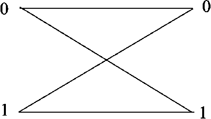
In this subsection, we use a 2-lossy and 2-valued channel as an example to explain the information theory analysis of a simple black-box channel. It is not difficult to generalize this analysis method to other k-lossy and $k^{'}$ -valued channels, including all the simple black-box channels in the experiments to follow.

Figure 1.

A 2-lossy and 2-valued channel with uniform distribution.

The channel in Fig. 1 is a 2-lossy and 2-valued channel. From the perspective of information theory, it is a binary symmetric channel with bit error probability 0.5, and uniform input and output bit probabilities. Let X be the channel input, Y be the channel output, and $P (Y | X)$ be the channel transition probability. Now, for the channel in Fig. 1, the input has entropy $H (X)$ , the output has entropy $H (Y)$ , and the joint entropy of the channel input and output is $H (X, Y)$ . The average mutual information is given by [5] $\begin{matrix} I (X; Y) = H (X) + H (Y) - H (X, Y) = H (X) - H (X | Y) = H (Y) - H (Y | X) . \end{matrix}$ Recalling the definitions in the previous section, it is easy to know that $λ_{L}$ is the input entropy, $H (X)$ , $λ_{T (L)}$ is the output entropy, and $λ_{L (T, L)}$ is the joint entropy, $H (X, Y)$ .

From the definitions of output and input lossy rates given previously, and using the relation between mutual information and entropy above, it follows that the output lossy rate, (i.e., $λ_{out} (L, T) = λ_{L (T, L)} - λ_{L}$ ), is $\begin{matrix} H (X, Y) - H (X) = H (Y) - I (X; Y) = H (Y | X), \end{matrix}$ and the input lossy rate, (i.e., $λ_{in} (L, T) = λ_{L (T, L)} - λ_{T (L)}$ ), is $\begin{matrix} H (X, Y) - H (Y) = H (X) - I (X; Y) = H (X | Y) . \end{matrix}$ In information theory terminology, the output lossy rate is the conditional entropy of output Y given input X, and reflects the average uncertainty in the transducer output given knowledge of the input. Similarly, the input lossy rate is the conditional entropy of transducer input X given the transducer output, Y.

4.1.2. Experiments using simple black-box channels

In the previous subsection, we have shown information theory analysis of simple black-box channels. In this subsection, we will conduct an array of experiments on these channels. We will also compare our experimental results to ideal results from theoretical analysis in order to demonstrate our experimental results as reasonable approximations of ideal values. The channels considered are diagrammed in Fig. 2, and in every case the channel input distribution is uniform, and the channel transition probabilities are uniform over the indicated links. For example, the binary symmetric channel in Fig. 2(d) has bit error probability 0.5.

Figure 2.

Structures of all transducers used in our experiments: (a) is a lossless and single-valued transducer; (b) is a 2-lossy and single-valued transducer; (c) is a lossless and 2-valued transducer; (d) is a 2-lossy and 2-valued transducer; (e) is 3-lossy and single-valued transducer; (f) is a lossless and 3-valued transducer; and (g) is a 3-lossy and 3-valued transducer.

The procedure of our experiments has four steps.

First, for a given (black-box) transducer, a sequence of symbols with length 100,000 is generated using a pseudo-random number generator as an input to the transducer. Then, we apply a “packing” method to encode as many input symbols as possible into one byte, subject to the input symbols being uniquely decoded from the packed bytes. (This is done for coding efficiency, since the commonly available LZ algorithm implementations, such as gzip [1], are byte-based.) As a result, the input sequence is converted into a packed input sequence. We use a Lempel–Ziv compression algorithm to compress the packed input sequence and obtain its compression ratio.

Second, the input sequence is fed to the transducer, symbol by symbol, to generate the output sequence. A nondeterministic choice in the transducer is simulated by a uniform probabilistic choice. Similarly to the previous step, we also apply the “packing” method to convert the output sequence into the packed output sequence. A Lempel–Ziv compression algorithm is used to compute the compression ratio of the packed output sequence.

Third, while the input sequence is fed to the transducer, we record every input symbol and the corresponding output symbol to obtain an input–output pair. As a result, a sequence of input–output pairs is generated. However, this process may not be length-preserving. Thus, to solve this problem, we use aforementioned shuffle coding to translate every input–output pair into a single symbol so that a new sequence, called a transducer sequence, is formed. Applying the packing approach in previous steps, the packed transducer sequence is generated. Again, a Lempel–Ziv algorithm is used and the compression ratio of the packed transducer sequence determined.

Fourth, we use the inverse of the compression ratios of the packed input sequence, the packed output sequence, and the packed transducer sequence to estimate, respectively, the information rates. Directly from their definitions, the input lossy rate and output lossy rate of the transducer are then calculated.

The experimental results are shown in Table 1. The transducers are implemented in Python. All of the experiments are performed on the Ubuntu 12.04 operating system.

Table 1

The estimated and ideal information rates for the input/output/transducer sequence of various transducers

Transducer type	Input		Output		Transducer

	Estimated	$H (X)$	Estimated	$H (Y)$	Estimated	$H (X, Y)$
(a) lossless and single-valued	1.004	1	1.004	1	1.004	1
(b) 2-lossy and single-valued	2.004	2	1.003	1	2.004	2
(c) lossless and 2-valued	1.003	1	2.004	2	2.004	2
(d) 2-lossy and 2-valued	1.003	1	1.003	1	2.004	2
(e) 3-lossy and single-valued	2.607	${log}_{2} 6$	1.003	1	2.607	${log}_{2} 6$
(f) lossless and 3-valued	1.003	1	2.606	${log}_{2} 6$	2.606	${log}_{2} 6$
(g) 3-lossy and 3-valued	1.611	${log}_{2} 3$	1.610	${log}_{2} 3$	3.222	${log}_{2} 9$

In Table 1, under the term “Input” (resp., “Output” and “Transducer”) is listed the estimated information rate (i.e., the inverse proportion of the compression ratio) of the input (resp., output and transducer) sequence. The columns immediately after each estimated information rate contain the ideal rate (the respective entropy).

In Table 2, under the term “Input lossy rate” (resp., “Output lossy rate”), two columns are listed: one includes the estimated input (resp., output) lossy rate of the corresponding transducer and the other one contains the ideal input (resp., output) lossy rate (respective conditional entropy) of the corresponding transducer. From the previous definitions, it is known that the input (resp., output) lossy rate of a transducer equals the information rate of its transducer sequence minus the information rate of its input (resp., output) sequence.

Table 2

The estimated input/output lossy rates of various transducers (bits/symbol)

Transducer type	Input lossy rate		Output lossy rate

	Estimated	$H (X \| Y)$	Estimated	$H (Y \| X)$
(a) lossless and single-valued	0	0	0	0
(b) 2-lossy and single-valued	1.001	1	0	0
(c) lossless and 2-valued	0	0	1.001	1
(d) 2-lossy and 2-valued	1.001	1	1.001	1
(e) 3-lossy and single-valued	1.604	${log}_{2} 3$	0	0
(f) lossless and 3-valued	0	0	1.603	${log}_{2} 3$
(g) 3-lossy and 3-valued	1.612	${log}_{2} 3$	1.611	${log}_{2} 3$

We summarize our findings from the experimental results as follows.

In Table 1, the estimated information rates in our simulation results are very close to their ideal values for every transducer. The largest difference between the experimental results and their ideal values are for the estimated information rates of the transducer sequence in case (g). The estimated information rate is only 1.6% larger than the ideal value. This case also corresponds to the least effective packing of symbols into bytes prior to LZ algorithm encoding. The results demonstrate that our approach provides reasonable estimates of information rates.

When the output lossy rate of a transducer is 0 (resp., positive), the transducer is likely single-valued (resp., k-valued ( $k > 1$ )). This finding is consistent with our definition. In a single-valued transducer (e.g., (a), (b) and (e) in Fig. 2), when the input sequence is given, the output sequence is unique. Thus, the information rates of the input sequence and the transducer sequence (using shuffle coding) are equal, so that the output lossy rate is 0. On the other hand, in a k-valued transducer, it is easy to show that its output lossy rate is positive.

When the input lossy rate of a transducer is 0 (resp., positive), the transducer is likely lossless (resp., k-lossy ( $k > 1$ )). The definition of a lossless transducer in this paper also reflects this fact. In a lossless transducer (e.g., (a), (c) and (f) in Fig. 2), two different input sequences cannot generate the same output sequence through the transducer. Similarly to the previous finding, using the shuffle coding, a one-to-one mapping can be built between the transducer sequence and the output sequence. Hence, the information rates of the transducer sequence and the output sequence are the same, i.e., the input lossy rate is 0. Similarly, a positive input lossy rate implies a k-lossy ( $k > 1$ ) transducer.

In a k-lossy ( $k > 1$ ) and $k^{'}$ -valued ( $k^{'} > 1$ ) transducer (e.g., (d) and (g) in Fig. 2), the information rate of the transducer sequence is larger than the information rate of the input sequence and the information rate of the output sequence. From the experimental results, it is also observed that in the k-lossy and $k^{'}$ -valued transducer cases, the information rates of the input sequence and the output sequence are almost equal and also approximately half of the information rate of the transducer sequence. This is simply due to the choice of uniform distribution of source symbols and uniform channel transition probabilities used in the experiments.

4.2. Complex black-box channels

In the previous subsection, we have shown how to use a Lempel–Ziv algorithm to estimate the input and output lossy rates of simple black-box channels. These channels were characterized by transducers that mapped a single input symbol to a single output symbol. The size of the input and output alphabets could be different, but the respective transducer mappings considered were fixed-length (single symbol) input to fixed-length (single symbol) output. It is rare to find such simple channels in computer programs, and so generally we are interested in transducers that are variable-length input to variable-length output mappings. We refer to these as nonfixed length channels, or simply as variable-length channels. So, before proceeding we need to outline how lossy information rates are estimated for the more general transducer channel model.

In this subsection, we will do our experiments on a compiler channel that is a compiler program treated as a variable-length input to variable-length output channel. Thus, in the following, we use a compiler channel as an example to explain the approximation approach for variable-length channels. In practice, it is known that for a compiler channel, the length of its input is always less than or equal to the length of its corresponding output. Obviously, it is not length preserving.

Figure 3.

A small part of a transducer sequence in a compiler channel.

To illustrate the concepts, consider the input to the compiler channel to be a C program, and the output the compiled assembly program. The input to the compiler channel consists of a sequence of input symbols. Every input symbol represents exactly one character (i.e. an ASCII character in the original input). A sequence of symbols is used to construct a statement, and a computer program is a sequence of statements. The compiler accepts a statement as input and generates one or more output statements. For example, Fig. 3 lists two input (C-code) statements and the resulting compiler output (assembly language). The first input statement (line 1) results in three lines of compiler output (lines 2–4), and the second input statement (line 5) results in one line of output (line 6). In this example, the input of the compiler channel only includes line 1 and line 5; the output of the compiler channel only contains lines 2–4 and line 6; the transducer sequence of the compiler channel includes all statements in this example and in the same format (i.e., every input statement is followed by its corresponding output statements). In every input statement (i.e., line 1 or line 5), every input symbol is a (ASCII) character. In every output statement (i.e., line 2–4 and line 6), every output symbol represents around 1.5 (ASCII) characters. Using this ratio, the number of input symbols equals the number of output symbols. It does not suggest that, for every input statement, the length of the corresponding output statement is 1.5 times of its length. It means, throughout the compiling process, every output symbol, at average, corresponds to around 1.5 (ASCII) characters in compiler output. (Note that, Fig. 3 only shows a small part of the complete transducer sequence. The ratio 1.5 is only determined by the length of the complete output file to the length of the complete input file. More details regarding the ratio will be defined and explained later.)

Through the channel, at the output side, every input symbol corresponds to exactly one output symbol. However, an output symbol may correspond to one or more output characters. Now, we may raise a question, how many characters can an output symbol represent? The answer depends on the program. We assume that, for a program, every output symbol represents the same number of characters in its output side. (Notice that the output symbol has a larger size of alphabet. For example, if a output symbol can represent two characters, then, the size of output symbols’ alphabet is the square of the size of the characters’ alphabet.) Hence, the number of characters represented by a output symbol is simply decided by the ratio of the length of the compiler’s output and the length of the compiler’s input. We call this value compiler ratio. The compiler ratio means the average number of characters represented by a output symbol, or says the average number of characters in output side generated by one character in the input side. Following these settings and assumptions, the compiler channel is length-preserving in input/output symbols format.

Now, we have a length-preserving channel and a compiler ratio for the channel. How can we compute the lossy rates? The key is determining how to compute the information rate of the output and the transducer (i.e., input–output pair) since the information rate of the input is computed as in previous experiments. We use the output side as an example to explain this. In the previous subsection, we have shown that the Lempel–Ziv algorithm can be used to approximate the information rate of the input/output on a length-preserving channel. Now, we use the same technique to compute the information rate of the output of the compiler channel in character format, rather than in output symbol format. But, under the length-preserving channel assumption, the output consists of output-symbols, not characters. Thus, we need to find a relation between the information rate of the output in character format and the information of the output in output symbol format. Then, we notice that every character-format sequence can be transformed into an output-symbol sequence by a one-to-one mapping. When an output-symbol represents m characters, the number of words in the output in characters format with length $n_{oc}$ (say $S_{n_{oc}}$ ), equals the number of words in the output in output symbol format with length $n_{os} = \frac{n_{oc}}{m}$ (say $S_{n_{os}}$ ). Hence, the information rate of the output in character format is as $\frac{1}{m}$ as the information rate of the output in output symbol format. Then, we have the following equation, $\begin{matrix} (1) & lim sup \frac{log S_{n_{oc}} (L_{oc})}{n_{oc}} = \frac{1}{m} \times lim sup \frac{log S_{n_{os}} (L_{os})}{n_{os}}, \end{matrix}$ where $L_{oc}$ is the set of output words in character format, $S_{n_{oc}} (L_{oc})$ denotes the number of words with length $n_{oc}$ , $L_{os}$ is the set of output words in output symbol format, $S_{n_{os}} (L_{os})$ denotes the number of words in $L_{os}$ with length $n_{os}$ , and m is the compiler ratio, i.e., the number of characters represented by a output-symbol. The way to compute the information rate of transducer (input–output pairs) is almost same. Therefore, we can use (1) and the definitions of lossy rates in the following experiments to estimate the lossy rates of a real world compiler.

Experiment subjects and setting. GCC is a commonly used compiler, and is a natural choice to use in our experiments. However, due to our device limitations, we cannot directly compile our programs on different architectures. Instead, we used a tool crosstool-ng, which also includes a GCC compiler inside, to conduct cross-compiling on a Linux machine so that crosstool-ng outputs assembly code that uses different architectures’ instruction sets.

The GNU coreutils is a collection of basic tools in Unix-like operating systems. It is also appropriate to use them as the inputs of the compiler. However, this toolset contains more than 100 programs, so that we do not have enough space to show results for all programs. Instead, we randomly chose 10 commonly used unix shell commands to present our results.

Experiment procedure. First, before compilation, each program is compressed using a Lempel–Ziv compression algorithm. Using its original length and compressed length, the compression ratio is obtained. Similarly to the previous experiments, the information rate of the input is approximated as proportional to the inverse of the compression ratio.

Second, we use crosstool-ng to compile all programs on four architectures: ARM, MIPS, PowerPC, and x86. Thus, for every C program, a different version of the assembly code is generated for each of the four platforms. In the process of compilation, two kinds of outputs are formed. One output is the assembly code on the corresponding architecture. The other is the combination of C source code and its corresponding assembly code on the same architecture, i.e., the input–output pair in the transducer. These outputs are used, in the next step, to compute the information rates of the output and transducer, respectively.

Third, after compilation for each program, we can compress its combined output (i.e., the output in the transducer side) and its pure assembly output to get corresponding compression ratios. Then, the information rates of the transducer and the output are computed. Because a compiler is non-length-preserving, we then compute compilation ratios for each type of output. Using Eq. (1), the information rates of the transducer and the output are obtained.

Fourth, using the definitions above, the lossy rates are also computed for each program.

Experimental results and findings. The experimental results are presented in Tables 3–6.

In each table, the term “Name” represents the program being compiled and the program is treated as a black-box channel. The term “Input lossy” (resp., “Output lossy”) indicates the input (resp., output) lossy rate of the corresponding channel. Each table’s name represents the architecture on which programs are compiled.

Table 3

ARM

Name	Input lossy	Output lossy
cat.c	0.3000	0.3837
cp.c	0.3059	0.4106
cut.c	0.3436	0.5366
date.c	0.3257	0.3915
ls.c	0.3080	0.4917
pwd.c	0.4167	0.5725
sort.c	0.3512	0.5240
tail.c	0.3699	0.6490
wc.c	0.3849	0.7422
who.c	0.3217	0.5937

Table 4

MIPS

Name	Input lossy	Output lossy
cat.c	0.3124	0.4214
cp.c	0.3235	0.4455
cut.c	0.3515	0.5432
date.c	0.3471	0.4264
ls.c	0.3174	0.5063
pwd.c	0.4522	0.7460
sort.c	0.3649	0.5852
tail.c	0.3786	0.6630
wc.c	0.4086	0.7799
who.c	0.3340	0.6012

Table 5

PowerPC

Name	Input lossy	Output lossy
cat.c	0.3757	0.6846
cp.c	0.3386	0.5856
cut.c	0.3334	0.5914
date.c	0.4876	0.7658
ls.c	0.2784	0.5046
pwd.c	0.4369	0.6777
sort.c	0.3197	0.5842
tail.c	0.3365	0.6012
wc.c	0.3090	0.5723
who.c	0.3741	0.6274

Table 6

x86

Name	Input lossy	Output lossy
cat.c	0.3937	0.6840
cp.c	0.3554	0.6131
cut.c	0.3373	0.6491
date.c	0.4598	0.7016
ls.c	0.2642	0.4719
pwd.c	0.4078	0.6198
sort.c	0.3241	0.5729
tail.c	0.3424	0.6119
wc.c	0.3253	0.5978
who.c	0.3663	0.6233

We summarize our findings from the experimental results as follows.

On each architecture, both input lossy rate and output lossy rate of each program are positive. It indicates that the compiling process is equivalent to a k-lossy ( $k > 1$ ) and $k^{'}$ -valued ( $k^{'} > 1$ ) channel (or transducer). (But, we may not find integers k and $k^{'}$ to satisfy lossy rates in the tables.) This finding is consistent with our understanding of a compiler. In the compiling process, two distinct symbols may be translated to the same symbol and the same symbol in different locations may be translated to different symbols.

As shown in Tables 3–6, for every architecture, and for every program, the output lossy rate is larger than the input lossy rate. This observation is interpreted as follows. For a compiler, the input is just a C program while the compiled output is an assembly program. It is well known that C is a high-level programming language while assembly language is a low-level programming language. To implement the same functionality, a C program only focuses on the control flow of its program and its high-level data structures, and many details in low-level (i.e. related to hardware architectures) are ignored, while all high-level control flows, data structures, as well as low-level details are included in an assembly program. Hence, we can say that a C program only includes high-level information and a assembly program combines high-level and low-level information together. This suggests that, for the same functionality, assembly programs contain more information than C programs. One interpretation is that a compiler adds “side-information” when processing an input. This side-information is hardware-specific and not required in a high-level (e.g., C) program, but necessary in the assembly language instructions that execute on a specific hardware processor.

Comparing Tables 3 and 4, we find that, for the same program, the values of the input lossy rates for the ARM architecture and for the MIPS architecture are very similar. In Tables 5 and 6, the input lossy rates for the PowerPC architecture and the x86 architecture are also similar in value. Reviewing all data generated in our experiments, we seek an explanation for this observation. For a channel, the input lossy rate is determined by two terms: the information rate of its transducer side and the information rate of its output. Both the transducer side and the output contain information from the output. Then, the amount of information in the output may be a key factor in the input lossy rate. We also know that the output depends on the architecture and hence the input lossy rate. This really says the input lossy rate of a channel reflects its architecture characteristics. Both ARM and MIPS use a RISC instruction set and are mainly used in mobile devices and embedded systems. Thus, their platform characteristics are similar, and we observe similar lossy input rates over a broad collection of C programs. Although PowerPC and x86 use different instruction sets, they are mainly designed for desktop PCs and server computers, and they also have some similar platform characteristics. Again, we observe similar lossy input rates over the collection of C programs, but rather distinctly different that for the ARM and MIPS architectures.

Through the above experiments, we demonstrate that the lossy rate in a channel is a useful analysis tool in practice. Note that in the previous experiments, the implementation of a compiler is unknown, and its structure is simply modeled as a black-box channel. Even with a black-box model, we still can use its external behaviors to compute the lossy rates of the channel and gain some knowledge regarding the channel’s properties.

Footnotes

Acknowledgements

We would like to thank Klaus Wich for pointing out to us that the finite-ambiguity problem for linear context-free grammars was shown undecidable in his PhD thesis, Eric Wang for comments that improved the presentation of our results, and the referees for their suggestions.

Supported in part by NSF Grants CCF-1143892 and CCF-1117708.

References

http://www.gzip.org/.

Alur and

D.L.

Dill , A theory of timed automata, Theoretical Computer Science 126(2) (1994), 183–235.

Asarin and

Degorre , Volume and entropy of regular timed languages: Discretization approach, in: CONCUR, 2009, pp. 69–83.

Chomsky and

G.A.

Miller , Finite state languages, Information and Control 1 (1958), 91–112.

T.M.

Cover and

J.A.

Thomas , Elements of Information Theory, 2nd edn, Wiley-Interscience, 2006.

Cui ,

Dang and

T.R.

Fischer , Bit rate of programs, CoRR, 2013.

Cui ,

Dang ,

T.R.

Fischer and

O.H.

Ibarra , Similarity in languages and programs, Theor. Comput. Sci. 498 (2013), 58–75.

Cui ,

Dang ,

T.R.

Fischer and

O.H.

Ibarra , Information rate of some classes of non-regular languages: An automata-theoretic approach, in: MFCS’14, Lecture Notes in Computer Science, Vol. 8634, Springer, 2014.

Dang , Pushdown timed automata: A binary reachability characterization and safety verification, Theor. Comput. Sci. 1–3(302) (2003), 93–121.

10.

Dang ,

O.H.

Ibarra ,

Bultan ,

R.A.

Kemmerer and

Su , Binary reachability analysis of discrete pushdown timed automata, in: CAV’00: Proceedings of International Conference on Computer Aided Verification, Lecture Notes in Computer Science, Vol. 1855, Springer, 2000, pp. 69–84.

11.

Dang ,

O.H.

Ibarra and

Li , Sampling a two-way finite automaton, in: Emergence, Complexity and Computation, Automata, Universality, Computation, Vol. 12, Springer, 2014.

12.

E.M.

Gurari and

O.H.

Ibarra , The complexity of decision problems for finite-turn multicounter machines, Journal of Computer and System Sciences 22 (1981), 220–229.

13.

E.M.

Gurari and

O.H.

Ibarra , A note on finite-valued and finitely ambiguous transducers, Math. Systems Theory 16 (1983), 61–66.

14.

J.E.

Hopcroft ,

Motwani and

J.D.

Ullman , Introduction to Automata Theory, Languages, and Computation, 1st edn, Addison-Wesley, 1979.

15.

O.H.

Ibarra , Reversal-bounded multicounter machines and their decision problems, Journal of the ACM 25(1) (1978), 116–133.

16.

O.H.

Ibarra ,

Dang ,

Egecioglu and

Saxena , Characterizations of catalytic membrane computing systems, in: Proceedings of the 28th International Symposium on Mathematical Foundations of Computer Science (MFCS 2003), Lecture Notes in Computer Science, Vol. 2747, Springer, 2003, pp. 480–489.

17.

F.P.

Kaminger , The noncomputability of the channel capacity of context-sensitive languages, Inf. Comput. 17(2) (1970), 175–182.

18.

Kuich , On the entropy of context-free languages, Information and Control 16(2) (1970), 173–200.

19.

Li and

Dang, Sampling automata and programs, Theoretical Computer Science 577 (2015), 125–140.

20.

Paun , Membrane Computing, an Introduction, Springer-Verlag, 2002.

21.

M.P.

Schützenberger , Sur les Relations Rationnelles, in: Automata Theory and Formal Languages 2nd GI Conference Kaiserslautern, May 20–23, 1975 Lecture Notes in Comput. Sci., Vol. 33, 1975, pp. 209–213.

22.

C.E.

Shannon and

Weaver , The Mathematical Theory of Communication, University of Illinois Press, 1949.

23.

Staiger , The entropy of Lukasiewicz-languages, in: Revised Papers from the 5th International Conference on Developments in Language Theory, DLT’01, Springer-Verlag, London, UK, 2002, pp. 155–165.

24.

Wang ,

Cui ,

Dang ,

T.R.

Fischer and

Yang , Zero-knowledge blackbox testing: Where are the faults, Int’l. J. Foundations of Computer Science 25(2) (2014), 196–218.

25.

Weber , On the valuedness of finite transducers, Acta Inf. 27(9) (1990), 749–780.

26.

Wich , Ambiguity functions of context-free grammars and languages, PhD thesis, 2004.

27.

Xie ,

Dang and

O.H.

Ibarra , A solvable class of quadratic Diophantine equations with applications to verification of infinite state systems, in: Proceedings of the 30th International Colloquium on Automata, Languages and Programming (ICALP 2003), Lecture Notes in Computer Science, Vol. 2719, Springer, 2003, pp. 668–680.

28.

Yang ,

Cui ,

Dang and

T.R.

Fischer , An information-theoretic complexity metric for labeled graphs, 2011, in review.