Degrees of sets having no subsets of higher m

Abstract

We consider sets without subsets of higher m- and $t t$ -degree, that we call m-introimmune and $t t$ -introimmune sets respectively. We study how they are distributed in partially ordered degree structures. We show that:

each computably enumerable weak truth-table degree contains m-introimmune $Π_{1}^{0}$ -sets;

each hyperimmune degree contains bi-m-introimmune sets.

Finally, from known results we establish that each degree a with

a^{'} ⩾ 0^{″}

covers a degree containing

t t

-introimmune sets.

Keywords

Many-one reducibility truth-table reducibility weak truth-table reducibility computably enumerable degrees hyperimmune degrees

1. Introduction

The question of the existence of sets of natural numbers without subsets of higher Turing degree, from now on degree, was posed for the first time by Miller in his Master’s Thesis [21]. Soare [27] and Cohen (unpublished) solved the problem by showing their existence. By [17] we know that such sets cannot be arithmetical and by [26] we know that they cannot even be hyperarithmetical. Namely, define an infinite set A rich if every degree above that of A is represented by a subset of A. Then:

Theorem 1.1 (Jockusch [17]).

Let A be not rich. Then every arithmetical set is A-computable.

Theorem 1.2 (Simpson [26]).

Let A be not rich. Then every hyperarithmetical set is A-computable.

Given a reflexive and transitive reducibility $⩽_{r}$ , an r-degree is the class ${B \subseteq N : A is r -equivalent to B}$ for some $A \subseteq N$ , where A is r-equivalent to B, in symbols $A \equiv_{r} B$ , if and only if $A ⩽_{r} B$ and $B ⩽_{r} A$ . The class of infinite sets having no subsets of higher r-degree includes the following class of sets: $\begin{matrix} (1) & {A \subseteq N : A is infinite and for every X \subseteq A with | A - X | = \infty it holds that A {⩽̸}_{r} X} . \end{matrix}$ In [9] the term r-introimmune was introduced to denote each set in the class displayed in (1). The existence of sets with a certain property suggests the natural question of understanding how they are distributed in some structure. In our case this includes, e.g., to discover the lowest possible complexity of an r-introimmune set in a given structure for a given reducibility $⩽_{r}$ . For example, if we consider the arithmetical hierarchy we know that for many-one reducibility $⩽_{m}$ there are m-introimmune sets in $Π_{1}^{0}$ [6,7], which is the smallest class of the hierarchy that can contain such sets. For weak truth-table reducibility $⩽_{w t t}$ we proved in [8] that there exists a $w t t$ -introimmune set in $Δ_{2}^{0}$ . This means that for every reducibility $⩽_{r}$ that implies $⩽_{w t t}$ there are r-introimmune sets in $Δ_{2}^{0}$ ; apart from $r = 1, m$ , we do not know if there are such r-introimmune sets in $Π_{1}^{0}$ . In this paper we try to study the distribution of m- and $t t$ -introimmune sets in the partially ordered degree structure. We say that a degree is r-introimmune if it contains an r-introimmune set. For example, from Simpson’s result quoted above [26] we know that $0^{(α)}$ does not cover any T-introimmune degree for every $α < ω_{1}^{C K}$ . While from [8] we know that $0^{'}$ covers a $w t t$ -introimmune degree. In general we can formulate the following problem: Given a reducibility $⩽_{r}$ , to classify the r-introimmune degrees. Or more weakly: Given a reducibility $⩽_{r}$ , what are the degrees that cover r-introimmune degrees. For one-one reducibility $⩽_{1}$ we observe in Corollary 3.3 that the class of 1-introimmune degrees coincides with the class of non-zero degrees. While for weak truth-table reducibility $⩽_{w t t}$ we observe in Section 5 that $0^{'}$ is a $w t t$ -introimmune degree. We say that a set is bi-r-introimmune if both the set and its complement are r-introimmune. In this paper we give the following results:

each non-zero computably enumerable $w t t$ -degree contains an m-introimmune $Π_{1}^{0}$ -set;

each hyperimmune degree contains a bi-m-introimmune set;

each degree a with $a^{'} ⩾ 0^{″}$ covers a $t t$ -introimmune degree.

In Section 3 we compare the class of m-introimmune sets with some other common classes of sets studied in computability theory. In Section 4 we prove both 1) and 2), in Section 5 we establish 3).

2. Notations and terminology

Our terminology is standard. For undefined notions we refer to any monograph on computability theory as, for example, [14,22,24,28]. We consider sets of naturals numbers, unless otherwise stated. The symbol $N$ denotes the set of natural numbers. Given two sets $A, B \subseteq N$ ,

$A - B$ denotes the set difference of A and B,

$\overline{A}$ denotes $N - A$ ,

$A \oplus B = {2 x : x \in A} \cup {2 x + 1 : x \in B}$ .

We identify each set A with its characteristic function, namely

\begin{matrix} A (x) = \{\begin{matrix} 1 & if x \in A, \\ 0 & if x \notin A . \end{matrix} \end{matrix}

We fix an acceptable enumeration

φ_{0}, φ_{1}, \dots

of all the partial Turing computable unary functions. For every

x, y, e, t \in N

we define

φ_{e, t} (x) = φ_{e} (x) = y

if the e-th Turing machine on input x halts in t or fewer steps and outputs y, undefined otherwise. Given two sets

A, B \subseteq N

we say that:

A is many-one reducible to B, in symbols $A ⩽_{m} B$ , if there is a computable function f such that $\begin{matrix} x \in A \Leftrightarrow f (x) \in B \end{matrix}$ for every $x \in N$ . If f is one-one then A is one-one reducible to B, in symbols $A ⩽_{1} B$ ;

A is weak truth-table reducible to B, in symbols $A ⩽_{w t t} B$ , if there is an oracle Turing machine M and a computable function $f : N \to N$ such that

M with oracle B computes A, and

for every $x \in N$ , M on input x asks oracle B only numbers less than $f (x)$ .

The degree of a set A is denoted by

{deg}_{T} (A)

0

denotes the degree of all the computable sets.

a^{'}

and

a^{″}

denote respectively the first and second Turing jump of degree a. We say that a degree b covers the degree a if

a ⩽ b

, where ⩽ is the partial order on degrees induced by Turing reducibility. A degree

a ⩽ 0^{'}

is high₁ if

a^{'} = 0^{″}

. A degree or

w t t

-degree is computably enumerable (c.e.) if it contains a computably enumerable set. We will give further notations where needed.

3. A comparison between m-introimmunity and some other properties

For one-one reducibility we have a characterization of 1-introimmunity in terms of a classical immunity property, while for many-one reducibility there is no a similar characterization.

Definition 3.1 (Immune set).

An infinite set is immune if and only if it does not include any infinite c.e. set; equivalently, if and only if it does not include any infinite computable set.

Proposition 3.2.
A set is 1-introimmune if and only if is immune.
Proof.
$(\Leftarrow)$ Let A be an infinite set and let $X \subseteq A$ be such that $A ⩽_{1} X$ (it is not necessary here $| A - X | = \infty$ ). Let f be a one-one computable function witnessing that $A ⩽_{1} X$ . Fix $x \in A$ ; then ${x, f (x), f (f (x)), \dots}$ is an infinite c.e. subset of A, so A is not immune.

$(\Rightarrow)$ This part has been proved in Proposition 3.1 in [8]. □
Corollary 3.3.
Each $a > 0$ contains a 1-introimmune set.
Proof.
A degree a contains an immune set if and only if $a > 0$ [12] (see also [24], page 498). □

For many-one reducibility we preliminarily observe that each class of sets closed with respect to the unary operator $A \oplus A$ is not contained in the class of m-introimmune sets, because $A \oplus A$ is not m-introimmune for any set A. Now, for the class of m-introimmune sets we prove that:
it strictly includes the class of r-cohesive sets and is strictly included in the class of immune sets;

it is incomparable with the classes of q-cohesive sets and hyperimmune sets;

it is incomparable with the class of effectively immune sets.
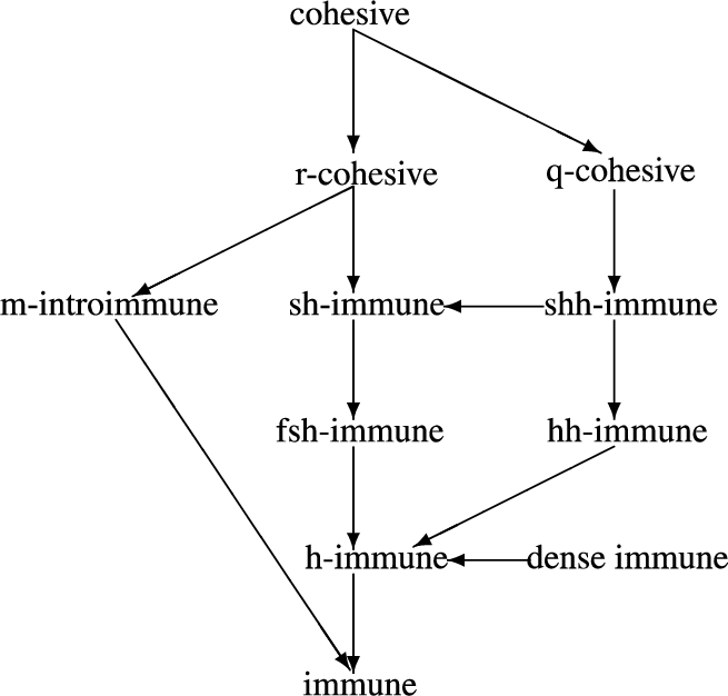
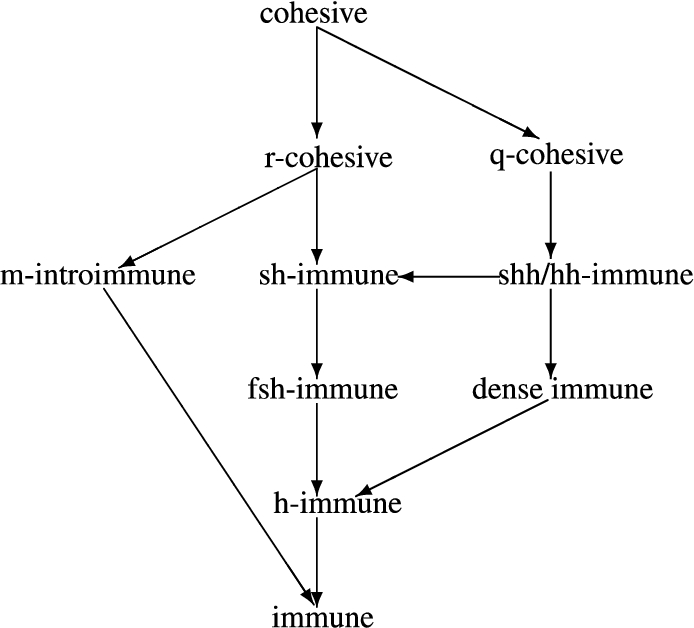
From (B) we conclude that the class of m-introimmune sets is incomparable with some other common classes of sets studied in computability theory; namely, is incomparable with the classes of strongly hyperimmune sets, strongly hyperhyperimmune sets, hyperhyperimmune sets, finitely strongly hyperimmune sets and dense immune sets. For the definitions of these sets we refer to [3,24,25,28]. We display in Diagram 1 and Diagram 2 the inclusions between these classes, in order to deduce the incomparability just listed.

Diagram 1.
The general case.

Diagram 2.
For $Π_{1}^{0}$ -sets.

We recall the definitions of the sets concerning (A), (B) and (C).
Definition 3.4 (Cohesive set, r-cohesive set, q-cohesive set, r-maximal set).

An infinite set A is

cohesive if there is no c.e. set W such that $A \cap W$ and $A \cap \overline{W}$ are both infinite;

r-cohesive if there is no computable set R such that $A \cap R$ and $A \cap \overline{R}$ are both infinite;

q-cohesive if it is a finite union of cohesive sets;

r-maximal if it is c.e. and its complement is r-cohesive.

Definition 3.5 (Hyperimmune set).

For every $n \in N$ let $D_{n}$ be the finite set with canonical index n. A disjoint strong array is a sequence ${D_{f (n)} : n ⩾ 0}$ where

f is a one-one computable function, and

for every $m \neq n$ , $D_{f (m)} \cap D_{f (n)} = \emptyset$ .

An infinite set H is hyperimmune if there is no disjoint strong array

{D_{f (n)} : n ⩾ 0}

such that

D_{f (n)} \cap H \neq \emptyset

for every n.

Definition 3.6 (Effectively immune set).

Fix a standard enumeration $W_{0}, W_{1}, \dots$ of all the c.e. sets. An infinite set E is effectively immune if there is a computable function φ such that for every $e \in N$ , if $W_{e} \subseteq E$ then $| W_{e} | ⩽ φ (e)$ .

3.1. (A)

Proposition 3.7.
The class of m-introimmune sets is strictly included in the class of immune sets.
Proof.
The inclusion is proved in Theorem 8(c) in [9]. The inclusion is strict because if A is immune then $A \oplus A$ is immune and not m-introimmune. □
Proposition 3.8.
The class of r-cohesive sets is strictly included in the class of m-introimmune sets.
Proof.
The inclusion is an immediate consequence of the proof of the following theorem due to Degtev: Theorem 3.9 (Degtev [10]; see also [23], Theorem 4.4).

If R is r-maximal then for every nontrivial superset S of R it holds that R and S are m-incomparable.

The proof of Theorem 3.9 shows that if C is any r-cohesive set and B is any infinite subsets of C such that $| C - B | = \infty$ , then C and B are m-incomparable. The inclusion is strict because bi-r-cohesive sets do not exist, while there are bi-m-introimmune sets (Theorem 4.10). Also, because the degree of an r-cohesive $Π_{1}^{0}$ -set is ${high}_{1}$ , while by Theorem 4.1 there are m-introimmune $Π_{1}^{0}$ -sets whose degree is not ${high}_{1}$ . □

3.2. (B)

Proposition 3.10.
The class of m-introimmune sets is incomparable with the class of hyperimmune sets.
Proof.
In the proof of Theorem 4.1 we construct an m-introimmune $Π_{1}^{0}$ -set which is not hyperimmune. Furthermore, if A is hyperimmune then $A \oplus A$ is hyperimmune and not m-introimmune. □
Proposition 3.11.
The class of m-introimmune sets is incomparable with the class of q-cohesive sets. In particular, the class of m-introimmune sets is not closed with respect to finite unions.
Proof.
Let C be a cohesive set and consider the two cohesive sets $2 C = {2 n : n \in C}$ and $2 C + 1 = {2 n + 1 : n \in C}$ . Since cohesive implies r-cohesive, by Proposition 3.8 $2 C$ and $2 C + 1$ are both m-introimmune; it follows that $2 C \cup (2 C + 1) = C \oplus C$ is q-cohesive and not m-introimmune.

The class of m-introimmune sets is not included in the class of q-cohesive sets, because otherwise it would be included in the class of hyperimmune sets, contrary to Proposition 3.10. □
3.3. (C)

Proposition 3.12.

There are m-introimmune sets that are not effectively immune.

There are effectively immune sets that are not m-introimmune.

Proof.

An effectively immune $Π_{1}^{0}$ -set can be only in $0^{'}$ [20] (see also Lemma 2.19.16 in [14], or Proposition III.2.18 in [24], or Theorem V.4.1 in [28]). By Theorem 4.1 there are m-introimmune $Π_{1}^{0}$ -sets not in $0^{'}$ .

If A is effectively immune then $A \oplus A$ is effectively immune and not m-introimmune. □

4. m-Introimmune and bi-m-introimmune sets

A degree is hyperimmune if it contains a hyperimmune set. In this section we prove that:

each non-zero c.e. $w t t$ -degree contains an m-introimmune $Π_{1}^{0}$ -set which is not hyperimmune, and

each hyperimmune degree contains a bi-m-introimmune set.

4.1. Computably enumerable $w t t$ -degrees and m-introimmune sets

Theorem 4.1.
Every non-zero c.e. $w t t$ -degree contains an m-introimmune $Π_{1}^{0}$ -set which is not hyperimmune.

Proof. We recall that a c.e. set is simple if its complement is immune. From [30] we know that every non-zero c.e. $w t t$ -degree contains a simple set (see [22], Theorem 1.7.3; see also either Proposition 2.13.1 in [14], or Proposition III.3.18 in [24], or Theorem V.3.2 in [28], taking into account that the c.e. permitting method used preserves reducibility $⩽_{w t t}$ ).

Therefore, to prove the statement of the theorem it is enough to fix any simple set A and build a c.e. set B such that $A \equiv_{w t t} B$ with $\overline{B}$ m-introimmune and not hyperimmune.

Let A be a simple set and fix a computable one-one enumeration $\begin{matrix} a_{0}, a_{1}, \dots \end{matrix}$ of A. Moreover, let $\begin{matrix} A = ⋃_{t ⩾ 0} A_{t}, \end{matrix}$ where $A_{0} = \emptyset$ and $\begin{matrix} A_{t} = {a_{0}, a_{1}, \dots, a_{t - 1}} \end{matrix}$ for every $t > 0$ . The construction of B is a combination of the finite-injury method with the c.e. permitting method that preserves reducibility $⩽_{w t t}$ . Precisely, we employ the permitting method based on Proposition 4.2 (see also either [14], or Theorem 1.7.2 in [22], or pp. 68 and 80 in [23], or Proposition V.3.1 in [28]). Proposition 4.2 (C.e. permitting method preserving $⩽_{w t t}$ ).

Let ${X_{t} : t ⩾ 0}$ and ${Y_{t} : t ⩾ 0}$ be two computable enumerations of the c.e. sets X and Y respectively. If $\begin{matrix} (\forall y) (\forall t) [y \in X_{t + 1} - X_{t} \Rightarrow (\exists a ⩽ y) (a \in Y - Y_{t})], \end{matrix}$ then $X ⩽_{w t t} Y$ .

4.1.1. Strategy

The construction of B is by infinitely many stages. At every stage t we define a finite approximation $B_{t}$ of B. The final set is $B = ⋃_{t ⩾ 0} B_{t}$ .

To make $A \equiv_{w t t} B$

We divide $N$ into infinitely many nonempty intervals $I_{0}, I_{1}, \dots$ , where

$I_{0} = {0, 1}$ ,

for every $n > 0$ , $I_{n}$ is the interval of ${(n + 1)}^{2} + 1$ numbers from $max (I_{n - 1}) + 1$ onwards.

Then, we guarantee that

for every $a \in N$ , $a \in A$ iff some element of $I_{a}$ is enumerated in B, and

we enumerate in $B_{t + 1}$ a number y if permitted by A, that is if $a_{t} ⩽ y$ .

Thus by i)

A ⩽_{w t t} B

and by ii)

B ⩽_{w t t} A

To make $\overline{B}$ not hyperimmune

Let f be a one-one computable function such that $D_{f (n)} = I_{a_{n}}$ for every $n ⩾ 0$ . We will ensure that at most ${(a_{n} + 1)}^{2}$ elements of $D_{f (n)}$ will be enumerated in B, obtaining $D_{f (n)} \cap \overline{B} \neq \emptyset$ for all n.

To make $\overline{B}$ m-introimmune

If φ is a computable function with $φ (x) = x$ for almost every x, then φ does not m-reduce an infinite set to any of its co-infinite subsets, so we do not care about this kind of functions. Hence in our construction we are interested in diagonalizing the computable functions φ with $φ (x) \neq x$ for infinitely many x.

Therefore we construct B in such a way that for every $e ⩾ 0$ the following requirement $R_{e}$ is satisfied:

$R_{e}$ : if $φ_{e}$ is computable and $φ_{e} (x) \neq x$ for infinitely many x, then

either there is a number $u \in \overline{B}$ with $φ_{e} (u) \in B$ , or

there are two numbers v, $v^{'}$ with $v \in B$ , $v^{'} \in \overline{B}$ and $φ_{e} (v) = φ_{e} (v^{'})$ .

Actions to satisfy each requirement

We informally describe the actions to satisfy each requirement. Fix $e ⩾ 0$ and let us suppose that $φ_{e}$ is computable and $φ_{e} (x) \neq x$ for infinitely many x. To satisfy $R_{e}$ we wait for a stage $t + 1$ at which we discover that there are two distinct numbers x, y not yet in $B_{t}$ and such that $\begin{matrix} (2) & either φ_{e, t} (x) = y or φ_{e, t} (x) = φ_{e, t} (y) . \end{matrix}$ Then we would like to keep x out of B and enumerate y in $B_{t + 1}$ . In this way $R_{e}$ would be satisfied because $φ_{e}$ does not many-one reduce $\overline{B}$ to any of its subsets. To keep x out of B we put a restraint $r_{e}$ on x. To enumerate y in $B_{t + 1}$ we have to check that y is not restrained by a higher priority requirement, i.e. $\begin{matrix} (3) & no restraint r_{d} with d < e is on y . \end{matrix}$ Furthermore, we must also ensure $B ⩽_{w t t} A$ , that is A must permit to enumerate y in $B_{t + 1}$ . In our case the permitting condition is that there is $s ⩽ t$ with $\begin{matrix} (4) & a_{s} ⩾ a_{t} and y \in I_{a_{s}}, \end{matrix}$ which implies $a_{t} ⩽ y$ . Accordingly, we enumerate y in $B_{t + 1}$ only if all the above conditions (2), (3) and (4) hold.

If at stage $t + 1$ A has not yet permitted $R_{e}$ to enumerate a number in B then we put, if possible, a restraint $r_{e}$ on a number $x \notin B_{t}$ of a pair $(x, y)$ of which both x and y are greater than all the numbers so far used by $R_{e}$ and such that (2) holds. In this way we start the generation of a sequence $(x_{0}, y_{0}), (x_{1}, y_{1}), \dots$ of pairs satisfying (2), with $r_{e}$ on each $x_{0}, x_{1}, \dots$ , and $\begin{matrix} (5) & y_{0} < y_{1} < \dots . \end{matrix}$ As we are assuming that $φ_{e} (x) \neq x$ for infinitely many x, the sequence (5) is potentially infinite. Since A is not computable, it will permit $R_{e}$ to enumerate some $y_{k}$ of (5) in B. In this way $φ_{e}$ is diagonalized and $R_{e}$ is satisfied if not later injured by some higher priority requirement by enumerating $x_{k}$ in B. However, the finite-injury priority method guarantees that eventually $R_{e}$ enumerates some element of (5) in B without being injured anymore.

4.1.2. Formalization of the construction of B

Every stage $t + 1$ of the construction consists of $a_{t} + 1$ iterations, in each of which we try to satisfy requirement $R_{e}$ , $0 ⩽ e ⩽ a_{t}$ , by putting the restraint $r_{e}$ on a number and enumerating in B another number, when possible. Furthermore, we must also guarantee that at the end of stage $t + 1$ is $I_{a_{t}} \cap B \neq \emptyset$ , in order to make $A ⩽_{w t t} B$ . If no number of $I_{a_{t}}$ is enumerated in B by the end of all the iterations $0, 1, \dots, a_{t}$ , then we choose the minimum number of $I_{a_{t}}$ with no restraints and enumerate it in B. To be sure that there exists such a number we impose that each requirement $R_{i}$ can put the restraint $r_{i}$ only on at most one element of each interval $I_{n}$ with $n > i$ ; in this way, at any time of the construction in each interval $I_{n}$ there can be at most $n < | I_{n} |$ elements with some restraint. Initially no restraint is used.

Construction of B

Stage 0. Set $B_{0} = \emptyset$ .

Stage $t + 1$ . Let $B_{t}$ be the set constructed by the end of stage t.

For $e = 0, 1, \dots, a_{t}$ do

Begin of the For-Loop

Let $B_{t, e}$ be the set of elements enumerated into B before running the iteration e of the loop. Go to the first case which applies. If there are several pairs $(x, y)$ satisfying the premises of the chosen case, then choose the length-lexicographical first such pair $(x, y)$ ; if no case applies, then just continue with the next iteration of the loop.

Case (a). If there are $x, y ⩽ t$ such that:

x has the restraint $r_{e}$ ,

$x \notin B_{t, e}$ and $y \in B_{t, e}$ ,

either $φ_{e, t} (x) = y$ or $φ_{e, t} (x) = φ_{e, t} (y)$ ,

then do nothing (that is set

B_{t, e + 1} = B_{t, e}

) and go to the next iteration of the loop.

Case (b). If there are distinct $x, y ⩽ t$ with $r_{e}$ on x and there is $s ⩽ t$ with $a_{s} ⩾ a_{t}$ such that:

$x \notin B_{t, e}$ and $y \in I_{a_{s}} - B_{t, e}$ ,

no restraint $r_{d}$ with $d < e$ is on y,

either $φ_{e, t} (x) = y$ or $φ_{e, t} (x) = φ_{e, t} (y)$ ,

then set

B_{t, e + 1} = B_{t, e} \cup {y}

and remove all the restraints on y. Go to the next iteration of the loop.

Case (c). Let a be the maximum of e and all b for which the interval $I_{b}$ contains some element used by $R_{e}$ at some previous stage. If there are distinct $x, y ⩽ t$ with:

$x, y \notin B_{t, e}$ ,

$min {x, y} > max (I_{a})$ ,

either $φ_{e, t} (x) = y$ or $φ_{e, t} (x) = φ_{e, t} (y)$ ,

then declare x and y used by

R_{e}

at this stage. Put the restraint

r_{e}

on x, set

B_{t, e + 1} = B_{t, e}

and go to the next iteration of the loop.

End of the For-Loop

If no element of $I_{a_{t}}$ has been enumerated in $B_{t, a_{t} + 1}$ , then choose the least $y \in I_{a_{t}}$ with no restraints and set $B_{t + 1} = B_{t, a_{t} + 1} \cup {y}$ ; otherwise set $B_{t + 1} = B_{t, a_{t} + 1}$ .

End of Stage $t + 1$ .

End of construction of B

Set $B = ⋃_{t ⩾ 0} B_{t}$ .

4.1.3. Verification

Clearly B is computably enumerable.

Lemma 4.3.
$\overline{B}$ is not hyperimmune.
Proof.
Recall that $D_{f (s)} = I_{a_{s}}$ for every s. Fix $s ⩾ 0$ . An element of $I_{a_{s}}$ is enumerated in B at some stage $t + 1$ only if $a_{s} ⩾ a_{t}$ . Condition $a_{s} ⩾ a_{t}$ can be true for at most $a_{s} + 1$ values of t. At each stage $t + 1$ for which $a_{s} ⩾ a_{t}$ there are at most $a_{t} + 1$ requirements $R_{e}$ , $e ⩽ a_{t}$ , that can enumerate in B an element of $I_{a_{s}}$ , therefore $\begin{matrix} | I_{a_{s}} \cap B | ⩽ (a_{s} + 1) (a_{t} + 1) ⩽ {(a_{s} + 1)}^{2} . \end{matrix}$ This implies that $I_{a_{s}} \cap \overline{B} \neq \emptyset$ because $| I_{a_{s}} | = {(a_{s} + 1)}^{2} + 1$ , hence $\overline{B}$ is not hyperimmune. □
Lemma 4.4.
$A \equiv_{w t t} B$ .
Proof.

$A ⩽_{w t t} B$ . If $a \in A$ , say $a = a_{t}$ , then at the end of stage $t + 1$ it is $B \cap I_{a_{t}} \neq \emptyset$ . Furthermore, only elements of $I_{a}$ with $a \in A$ are enumerated in B. It follows that $a \in A$ if and only if $I_{a} \cap B \neq \emptyset$ , which implies $A ⩽_{w t t} B$ .

$B ⩽_{w t t} A$ . For every $y, t ⩾ 0$ , $\begin{matrix} y \in B_{t + 1} - B_{t} \Rightarrow y \in I_{a_{s}} with a_{s} ⩾ a_{t}, that is a_{t} ⩽ y . \end{matrix}$ Since $a_{t} \in A - A_{t}$ , $B ⩽_{w t t} A$ by Proposition 4.2. □

Lemma 4.5.
$\overline{B}$ is m-introimmune.
Proof.
$\overline{B}$ is infinite because $D_{f (n)} \cap \overline{B} \neq \emptyset$ for every $n ⩾ 0$ . We have to prove that each requirement is met. We say that requirement $R_{e}$ requires attention at stage $t + 1$ if in the iteration $e ⩽ a_{t}$ one of the cases (b) or (c) of the construction of B applies. We prove in Proposition 4.7 that each requirement requires attention at most finitely often and in Proposition 4.9 that each requirement is met. To prove Proposition 4.7 we need the following result first. Proposition 4.6.
$⋃_{t ⩾ 0} I_{a_{t}}$ is simple.
Proof.
Clearly $⋃_{t ⩾ 0} I_{a_{t}}$ is computably enumerable. It is not computable because $\begin{matrix} A ⩽_{1} ⋃_{t ⩾ 0} I_{a_{t}} \end{matrix}$ via the computable function $g (n) = min (I_{n})$ , in particular $\overline{⋃_{t ⩾ 0} I_{a_{t}}}$ is infinite. For the sake of contradiction, let us suppose that $\overline{⋃_{t ⩾ 0} I_{a_{t}}}$ is not immune. Let W be an infinite c.e. subset of $\overline{⋃_{t ⩾ 0} I_{a_{t}}}$ and define the c.e. set $\begin{matrix} \hat{W} = {n : I_{n} \cap W \neq \emptyset} . \end{matrix}$ $\hat{W}$ is infinite because ${I_{n}}_{n ⩾ 0}$ is a partition of $N$ and each $I_{n}$ is finite. Furthermore $\hat{W}$ is a subset of $\overline{A}$ , contradicting A simple: given $m \in N$ , $\begin{matrix} m \in \hat{W} \Rightarrow I_{m} \cap W \neq \emptyset, \end{matrix}$ from which $\begin{matrix} I_{m} ⊈ ⋃_{t ⩾ 0} I_{a_{t}}; \end{matrix}$ then $m \neq a_{t}$ for every $t ⩾ 0$ , and $m \in \overline{A}$ . □
Proposition 4.7.
Each requirement requires attention at most finitely often.
Proof.
Assume by way of contradiction that e is the least index for which $R_{e}$ requires attention infinitely many often and let $t_{0}$ be the minimum stage after which no requirement $R_{i}$ with $i < e$ requires attention. If at some stage $t + 1 ⩾ t_{0}$ in the iteration e one of cases (a) or (b) applies then at the end of stage $t + 1$ there is a pair $(x, y)$ satisfying the following conditions: $\begin{array}{l} – x has restraint r_{e}, \\ – x \notin B_{t + 1} and y \in B_{t + 1}, \\ – either φ_{e, t} (x) = y or φ_{e, t} (x) = φ_{e, t} (y) . \end{array}$ By hypothesis on $t_{0}$ the restraint $r_{e}$ on x is not removed, that to say that after stage $t + 1$ only case (a) can apply and $R_{e}$ does not require attention anymore, contradicting the hypothesis that $R_{e}$ requires attention infinitely often.

Therefore the iteration e goes in infinitely many stages through case (c). This means that there is an infinite sequence ${(x_{k}, y_{k}) : k ⩾ 0}$ such that each $x_{k}$ carries the restraint $r_{e}$ and $\begin{matrix} y_{0} < y_{1} < \dots, \end{matrix}$ that to say that ${y_{k} : k ⩾ 0}$ is an infinite computable set. As $⋃_{t ⩾ 0} I_{a_{t}}$ is simple, for every $k_{0} \in N$ it holds that $\begin{matrix} | {y_{k} : k ⩾ k_{0}} \cap (⋃_{t ⩾ 0} I_{a_{t}}) | = \infty . \end{matrix}$ By hypothesis on $t_{0}$ we can choose $k_{0}$ in such a way that no restraint $r_{d}$ with $d < e$ is on $y_{k}$ for every $k ⩾ k_{0}$ . Then Fact 4.8.
A is computable.
Proof.
Given $a ⩾ e$ , find a stage $t + 1 > t_{0}$ such that there is $s ⩽ t$ with $a_{s} ⩾ a$ and $y_{k} \in I_{a_{s}}$ for some $k ⩾ k_{0}$ . Then we show that $\begin{matrix} a \in A \Leftrightarrow a \in {a_{0}, a_{1}, \dots, a_{t}} . \end{matrix}$ For the sake of contradiction, if $a \in A - {a_{0}, a_{1}, \dots, a_{t}}$ then there exists $t^{'} > t$ such that $a = a_{t^{'}}$ . Thus at stage $t^{'} + 1$ there is $s ⩽ t^{'}$ with $a_{s} ⩾ a_{t^{'}} = a$ and $y_{k} \in I_{a_{s}}$ . Observe that there is no an intermediate stage $t^{″}$ between $t + 1$ and $t^{'} + 1$ at which $y_{k}$ is enumerated in B. Otherwise, by hypothesis on $t_{0}$ , from $t^{″}$ onwards the pair $(x_{k}, y_{k})$ will satisfy the premises of case (a) of the algorithm in each iteration e, contradicting the generation of the infinite sequence ${(x_{k}, y_{k}) : k ⩾ 0}$ . By hypothesis on $k_{0}$ no restraint $r_{d}$ with $d < e$ can be on $y_{k}$ , hence in the iteration e of stage $t^{'} + 1$ it holds that $x_{k}$ and $y_{k}$ satisfy the premises of case (b) of the algorithm, i.e.: $\begin{array}{l} – x_{k} \notin B_{t^{'}, e} and y_{k} \in I_{a_{s}} - B_{t^{'}, e} \\ – no restraint r_{d} with d < e is on y_{k} \\ – either φ_{e, t^{'}} (x_{k}) = y_{k} or φ_{e, t^{'}} (x_{k}) = φ_{e, t^{'}} (y_{k}) . \end{array}$ Consequently $y_{k}$ is enumerated in $B_{t^{'}, e + 1}$ . After stage $t^{'} + 1$ no requirement can eliminate $r_{e}$ on $x_{k}$ . Thus, after stage $t^{'} + 1$ the pair $(x_{k}, y_{k})$ will satisfy the premises of case (a). This means that $R_{e}$ does not require attention after $t^{'} + 1$ , contradicting the generation of the infinite sequence ${(x_{k}, y_{k}) : k ⩾ 0}$ . This concludes the proof of Fact 4.8. □

But A computable contradicts A simple. This concludes the proof of Proposition 4.7. □
Proposition 4.9.
Every requirement is met.
Proof.
For the sake of contradiction, let e be the minimum such that $R_{e}$ is not met and let C be a subset of $\overline{B}$ such that $| \overline{B} - C | = \infty$ and $\overline{B} ⩽_{m} C$ via $φ_{e}$ . Since $| \overline{B} - C | = \infty$ , it is necessarily $φ_{e} (x) \neq x$ for infinitely many x. Let $t_{0}$ be the minimum stage after which no requirement $R_{d}$ with $d < e$ requires attention. As $φ_{e}$ many-one reduces $\overline{B}$ to C, there are infinitely many distinct $x, y \in \overline{B}$ for which either $φ_{e} (x) = y$ or $φ_{e} (x) = φ_{e} (y)$ . The second case occurs if infinitely many $x \in \overline{B}$ are mapped to the same element, while the first case occurs if the mapping $φ_{e}$ is only finite-to-one on the elements of $\overline{B}$ . If at some stage $t + 1 ⩾ t_{0}$ one of cases (a) or (b) of the construction of B applies then there is a pair $(x, y)$ with $x \notin B_{t + 1}$ , $y \in B_{t + 1}$ , $r_{e}$ on x and either $φ_{e} (x) = y$ or $φ_{e} (x) = φ_{e} (y)$ . By hypothesis on $t_{0}$ no requirement enumerates x in B after $t + 1$ , which implies that $φ_{e}$ does not many-one reduce $\overline{B}$ to C, contradicting $\overline{B} ⩽_{m} C$ via $φ_{e}$ .

Therefore after stage $t_{0}$ case (c) would apply infinitely often, but this contradicts Proposition 4.7. □

This concludes the proof of Lemma 4.5. □

This concludes the proof of Theorem 4.1. □
4.2. Hyperimmune degrees and bi-m-introimmune sets

Since m-introimmunity implies immunity, not all degrees contain a bi-m-introimmune set because there is a non-zero degree $a ⩽ 0^{″}$ such that every degree covered by a is bi-immune free (Jockusch [15], cf. Theorem 1). Here we show that every hyperimmune degree contains a bi-m-introimmune set. Precisely, we show that each Kurtz random set is bi-m-introimmune; the result follows since every hyperimmune degree contains a Kurtz random set. The class of degrees containing a bi-m-introimmune set is wider than the class of hyperimmune degrees, because there are hyperimmune free degrees containing Kurtz random sets: see the discussion immediately after Corollary 8.11.8 in [14]. At the moment we do not know what the exact extension of the class of degrees containing a bi-m-introimmune set is.

Theorem 4.10.
Every Kurtz random set is bi-m-introimmune.
Proof.
We introduce first a couple of concepts. Definition 4.11.
A function $f : N \to N$ is one-one almost everywhere if and only if the set $\begin{matrix} {(x, y) : x \neq y \land f (x) = f (y)} \end{matrix}$ is finite.
Definition 4.12 (Balcázar, Díaz and Gabarró [4], Balcázar and Schöning [5]).

A set S is strongly bi-immune if and only if every many-one reduction of S to any set is one-one almost everywhere.

We prove first that each Kurtz random set is strongly bi-immune. Then we prove that each strongly bi-immune set is bi-m-introimmune. There are several characterizations of the notion of Kurtz randomness [13]; here we use the martingale characterization. Let us introduce first the following terminology. A string is a finite, possibly empty, sequence of 0’s and 1’s. If α is a string and $b \in {0, 1}$ , then $α b$ denotes the concatenation of α followed by b. For every set $X \subseteq N$ and for every positive $n \in N$ we denote with $X ↾ n$ the string $\begin{matrix} X (0) X (1) \dots X (n - 1) . \end{matrix}$ $X ↾ 0 = \emptyset$ is the empty string.

Definition 4.13 (Martingale).

Let $R^{⩾ 0}$ be the set of nonnegative real numbers and let ${0, 1}^{*}$ be the set of strings. A martingale is a function $\begin{matrix} F : {0, 1}^{*} \to R^{⩾ 0} \end{matrix}$ such that for all $α \in {0, 1}^{*}$ $\begin{matrix} 2 F (α) = F (α 0) + F (α 1) . \end{matrix}$

In the following definition we give the characterization of Kurtz randomness in terms of martingales. This characterization has been proved in [29] (see also Theorem 4 in [13], or Theorem 7.2.13 in [14]).

Definition 4.14 (Kurtz random set).

A set $X \subseteq N$ is Kurtz random if and only if there is no computable martingale F such that $F (X ↾ n) ⩾ h (n)$ for almost all n, where $h : N \to N$ is an unbounded, non decreasing, computable function.

Proposition 4.15.
Every Kurtz random set is strongly bi-immune.
Proof.
Let us suppose that A is not strongly bi-immune. Then A is many-one reducible to some set via a computable function $f : N \to N$ with $\begin{matrix} (6) & | {(x, y) : x \neq y \land f (x) = f (y)} | = \infty . \end{matrix}$ Fix such an f.
Betting strategy

A betting strategy to win an infinite gain on A is the following. Let us suppose that we saw the first n values $\begin{matrix} A (0), A (1), \dots, A (n - 1) \end{matrix}$ and that our capital is $F (A ↾ n) > 0$ . We have to decide how to bet on the $(n + 1)$ -th value $A (n)$ . We first compute $f (n)$ and then we check whether or not there is $j < n$ such that $f (j) = f (n)$ . If such a j exists then we know that the $(n + 1)$ -th value $A (n)$ is equal to $A (j)$ , because f is a many-one reduction of A to some set. In this case we bet $F (A ↾ n)$ on $A (n) = A (j)$ , increasing our capital to $2 F (A ↾ n)$ . Otherwise we bet 0, keeping the capital $F (A ↾ n)$ . By (6) we have infinitely many chances to double our capital; since f is a many-one reduction of A to some set, we have no chances to loose it.
Formalization

For every $n \in N$ let us define $\begin{matrix} J_{n} = {j : j < n \land f (j) = f (n)} . \end{matrix}$ Let us define the computable function $F : {0, 1}^{} \to R^{⩾ 0}$ as follows: $F (\emptyset) = 1$ ; for every $n ⩾ 0$ , for every $X \subseteq N$ and every $b \in {0, 1}$ $\begin{matrix} F ((X ↾ n) b) = \{\begin{matrix} 2 F (X ↾ n) & if J_{n} \neq \emptyset and the min (J_{n}) -th element of X ↾ n is b, \\ 0 & if J_{n} \neq \emptyset and the min (J_{n}) -th element of X ↾ n is not b, \\ F (X ↾ n) & if J_{n} = \emptyset . \end{matrix} \end{matrix}$ Fact 4.16.
F is a martingale.*
Proof.
Fix $n ⩾ 0$ and distinguish two cases on $J_{n}$ .
$J_{n} = \emptyset$ . In this case $F (X ↾ n) = F ((X ↾ n) 0) = F ((X ↾ n) 1)$ .

$J_{n} \neq \emptyset$ . In this case let us suppose first that the $min (J_{n})$ -th element of $X ↾ n$ is 0. Then $\begin{matrix} F ((X ↾ n) 0) = 2 F (X ↾ n) \end{matrix}$ and $\begin{matrix} F ((X ↾ n) 1) = 0 . \end{matrix}$ The case in which the $min (J_{n})$ -th element of $X ↾ n$ is 1 is symmetric. Thus in both cases (a) and (b) it holds that $\begin{matrix} 2 F (X ↾ n) = F ((X ↾ n) 0) + F ((X ↾ n) 1) . \end{matrix}$
This concludes the proof of Fact 4.16. □

Let us define the computable function $h : N \to N$ as $h (0) = 1$ and for every $n ⩾ 0$ $\begin{matrix} h (n + 1) = \{\begin{matrix} 2 h (n) & if J_{n} \neq \emptyset, \\ h (n) & otherwise. \end{matrix} \end{matrix}$ Clearly h is non decreasing; by (6) there are infinitely many n with $J_{n} \neq \emptyset$ , hence h is unbounded. Furthermore, Fact 4.17.
$F (A ↾ n) = h (n)$ for every $n ⩾ 0$ .
Proof.
By induction on n. Clearly $F (A ↾ 0) = F (\emptyset) = 1 = h (0)$ . Fix $n + 1$ and let us suppose that $F (A ↾ n) = h (n)$ . Distinguish two cases on $J_{n}$ .
$J_{n} \neq \emptyset$ . For all $j \in J_{n}$ is $A (j) = A (n)$ since f is a many-one reduction of A to some set. Then the $min (J_{n})$ -th element of $A ↾ n$ is $A (n)$ . We have that $\begin{matrix} F ((A ↾ n) A (n)) = 2 F (A ↾ n) = 2 h (n) = h (n + 1) . \end{matrix}$ But $F ((A ↾ n) A (n)) = F (A ↾ (n + 1))$ , thus $\begin{matrix} F (A ↾ (n + 1)) = h (n + 1) . \end{matrix}$

$J_{n} = \emptyset$ . In this case $\begin{matrix} F (A ↾ (n + 1)) = F ((A ↾ n) A (n)) = F (A ↾ n) = h (n) = h (n + 1) . \end{matrix}$
This concludes the proof of Fact 4.17. □

In conclusion, martingale F and h certify that A is not Kurtz random. This concludes the proof of Proposition 4.15. □
Proposition 4.18.
Every strongly bi-immune set is bi-m-introimmune.
Proof.
Let A be strongly bi-immune; then A cannot be computable. For the sake of contradiction and without loss of generality let us suppose that A is not m-introimmune. Let $B \subseteq A$ with $| A - B | = \infty$ and $A ⩽_{m} B$ via g. By hypothesis g is one-one almost everywhere, so there are at most finitely many $x \in A - B$ with ${x, g (x), g (g (x)), \dots}$ finite. Let $x \in A - B$ be such that ${x, g (x), g (g (x)), \dots}$ is infinite; such set is c.e., which means that there is an infinite computable set $R \subseteq A$ . Fix $a \in A - R$ . Then A is many-one reducible to $A - R$ via $\begin{matrix} f (x) = \{\begin{matrix} a & if x \in R, \\ x & if x \notin R . \end{matrix} \end{matrix}$ Function f is not one-one almost everywhere because $\begin{matrix} {(x, y) : x \neq y \land x, y \in R \land f (x) = f (y) = a} \end{matrix}$ is infinite. This concludes the proof of Proposition 4.18. □

This concludes the proof of Theorem 4.10. □
Corollary 4.19.
Each hyperimmune degree contains a bi-m-introimmune set. In particular, each non-zero c.e. degree contains a bi-m-introimmune set.
Proof.
Each hyperimmune degree contains a Kurtz random set [18] (see also either Corollary 8.11.8 in [14], or Remark 3.5.3.(i) in [22]). Furthermore, each non-zero c.e. degree contains a hyperimmune set [11] (see also either Proposition 1.7.6 in [22], or Proposition III.3.13 in [24], or Theorem V.2.5 in [28]). □

5. $t t$ -Introimmune degrees

In this last section we continue with our general project to understand how r-introimmune sets are distributed in the partially ordered degree structure for a given reducibility $⩽_{r}$ . This project includes, for example, understanding how low can the complexity of an r-introimmune set be.

In [8] we constructed a $w t t$ -introimmune set A with ${deg}_{T} (A) ⩽ 0^{'}$ . Actually the construction automatically shows that ${deg}_{T} (A) = 0^{'}$ by extending the notion of dominating function to all the partial computable functions, namely replacing Definition 3.3 in [8] with the following

Definition 5.1 (Dominating function).

A function $g : N \to N$ is dominating if for every partial computable function φ, $\begin{matrix} φ (n) is defined \Rightarrow φ (n) < g (n) \end{matrix}$ holds for almost every n.

The above set A is a subset of ${h (0), h (1), \dots}$ , where h is an increasing dominating function. Let $p_{A}$ be the principal function of A, that is $\begin{matrix} A = {p_{A} (0) < p_{A} (1) < \dots}; \end{matrix}$ then $p_{A}$ is dominating, thus $0^{'} ⩽ {deg}_{T} (A)$ too. However, we do not know if the bound $0^{'}$ can be lowered. For truth-table reducibility the bound $0^{'}$ can be lowered down to each ${high}_{1}$ degree at least in a weaker form, in the sense that each ${high}_{1}$ degree covers a $t t$ -introimmune degree. Let us first give the definition of truth-table reducibility. Fix an effective enumeration $\begin{matrix} σ_{0}, σ_{1}, \dots \end{matrix}$ of all the propositional formulas on the propositional variables $p_{0}, p_{1}, \dots$ . A set $D \subseteq N$ satisfies a propositional formula σ, in symbols $D ⊧ σ$ , if σ is true with $p_{n}$ interpreted as “ $n \in D$ ”.

Definition 5.2 (Truth-table reducibility).

Given two sets $A, B \subseteq N$ , A is truth-table reducible to B, in symbols $A ⩽_{t t} B$ , if there is a computable function f such that for every $x \in N$ $\begin{matrix} x \in A \Leftrightarrow B ⊧ σ_{f (x)} . \end{matrix}$

More generally it is possible to establish that each degree a with $a^{'} ⩾ 0^{″}$ covers a $t t$ -introimmune degree. This result is a corollary of a theorem in [1]. We say that an oracle Turing machine M is total if $M^{X} (x)$ is defined for every oracle X and every input x.

Definition 5.3 (Presentable reducibility [1], cf. Definition 4).

Let $⩽_{r}$ be a reducibility defined by $\begin{matrix} (\forall A, B) [A ⩽_{r} B \Leftrightarrow (\exists e) (A = M_{e}^{B})], \end{matrix}$ where ${M_{e} : e ⩾ 0}$ is a (computable) enumeration of total oracle Turing machines. Then $⩽_{r}$ is (computably) presentable and ${M_{e} : e ⩾ 0}$ is a (computable) presentation of $⩽_{r}$ .

Theorem 5.4 (Ambos-Spies [1], cf. Theorem 5).

Let $⩽_{r}$ be a presentable reducibility. There is an r-introimmune set A which is computable in the presentation of $⩽_{r}$ .

From Theorem 5.4 we get

Theorem 5.5.
Each degree a with $a^{'} ⩾ 0^{″}$ covers a $t t$ -introimmune degree.
Proof. We give a detailed proof. Let us recall the notion of an a-uniform enumeration for a class of unary functions (see also either [16] or Definition XII.3.3 in [28]).
Definition 5.6 (a-uniform enumeration).

Given a degree a, an enumeration $\begin{matrix} f_{0}, f_{1}, \dots \end{matrix}$ of unary functions is a-uniform if there is a function $f : N \times N \to N$ of degree $⩽ a$ such that $\begin{matrix} f (i, x) = f_{i} (x) \end{matrix}$ for every $i, x \in N$ .

Fix a degree a with $a^{'} ⩾ 0^{″}$ and take an a-uniform enumeration $\begin{matrix} (7) & f_{0}, f_{1}, \dots \end{matrix}$ of all the computable unary functions, whose existence has been proved by Jockusch [16] (see also Exercise XI.1.4.(b) in [25], or Theorem XII.3.4 in [28]). Enumeration (7) provides an a-computable presentation ${M_{e} : e ⩾ 0}$ of $⩽_{t t}$ by posing $\begin{matrix} M_{e}^{X} (x) = 1 \Leftrightarrow X ⊧ σ_{f_{e} (x)} \end{matrix}$ for every $e, x \in N$ and $X \subseteq N$ , where the numbers asked to the oracle X do not depend on X. These considerations allow us to obtain our result, which refines the existence of $t t$ -introimmune $Δ_{2}^{0}$ -sets ([1], cf. Corollary 6). Let us consider the function $h : N \to N$ defined as $h (0) = 0$ and $\begin{matrix} h (s + 1) = max_{i, j ⩽ h (s)} {z : M_{i} (j) asks z} + s + 1 . \end{matrix}$ Function h is a-computable, is increasing and satisfies the following property: for every $s ⩾ 0$ $\begin{matrix} (8) & (\forall m, e ⩽ s) M_{e} (h (m)) asks only numbers less than h (s + 1) . \end{matrix}$ We construct an infinite set $A \subseteq {h (0), h (1), \dots}$ by the finite extension method. At every stage s we define a finite set $A_{s}$ and the final set is $A = ⋃_{s ⩾ 0} A_{s}$ . The requirements are the following:

$P_{e}$ : $| A | ⩾ e$ ,

$N_{e}$ : for every $X \subseteq A$ with $| A - X | = \infty$ , $M_{e}$ is not a $t t$ -reduction of A to X.

5.1. Strategy

To satisfy $P_{e}$ we put an element in A at e stages. To satisfy $N_{e}$ we wait for a stage $s + 1 > e$ such that the following conditions i) and ii) hold:

for some $X \subseteq A_{s} \subseteq {h (0), h (1), \dots, h (s - 1)}$ it seems that $A_{s} ⩽_{t t} X$ via $M_{e}$ : $\begin{array}{l} h (0) \in A_{s} \Leftrightarrow M_{e}^{X} (h (0)) = 1, \\ h (1) \in A_{s} \Leftrightarrow M_{e}^{X} (h (1)) = 1, \\ ⋮ \\ h (s - 1) \in A_{s} \Leftrightarrow M_{e}^{X} (h (s - 1)) = 1; \end{array}$

$M_{e}^{X} (h (s)) = 1$ .

Then we make

M_{e}^{X} (h (s))

wrong by putting

h (s)

\overline{A}

. Note that by (8) the condition

s + 1 > e

implies that

\begin{matrix} (9) & M_{e} (h (s)) asks only numbers less than h (s + 1) . \end{matrix}

From (9), for every

B \subseteq A

the computation of

M_{e}^{B} (h (s))

does not depend on

B (h (s + 1)), B (h (s + 2)), \dots

. To facilitate the construction of A and subsequent proofs we introduce further notations on strings.

For a string α we denote with $| α |$ its length. If α is a string and $n < | α |$ , then $α (n)$ is the n-th value of α. We identify a string α with the finite set $\begin{matrix} X_{α} = {h (n) : n < | α | \land α (n) = 1} . \end{matrix}$ We write:

$α ⊑ β$ if α is a prefix of β, that is $\begin{matrix} | α | ⩽ | β | and α (i) = β (i) \end{matrix}$ for every $i < | α |$ ;

$α ⊏ β$ if $α ⊑ β$ and $α \neq β$ ;

$α \subseteq β$ if $| α | ⩽ | β |$ and $X_{α} \subseteq X_{β}$ , that is $\begin{matrix} α (i) ⩽ β (i) \end{matrix}$ for every $i < | α |$ .

In the construction of the set A at every stage s we define a string

α_{s}

of length s denoting the set

A_{s} = X_{α_{s}}

5.2. Requirements requiring attention

Fix a stage $s + 1$ and let $α_{s}$ be the string of length s constructed by the end of stage s. We say that:

$P_{e}$ requires attention at stage $s + 1$ if it is still not satisfied.

$N_{e}$ requires attention at stage $s + 1$ via the string $α \subseteq α_{s}$ , α of length s, if $s + 1 > e$ and the following conditions hold, which are the formalizations of the conditions i) and ii) described above:

C1: $(\forall m < s) [α_{s} (m) = M_{e}^{α} (h (m))]$ ,

C2: $M_{e}^{α 0} (h (s)) = 1$ .

5.3. Construction of A

Begin of construction

Stage 0. Set $α_{0} = \emptyset$ .

Stage $s + 1$ . Let $α_{s}$ be the string of length s constructed by the end of stage s and let n be the minimum such that $R_{n}$ requires attention. If $R_{n} = P_{n}$ then set $α_{s + 1} = α_{s} 1$ , otherwise set $α_{s + 1} = α_{s} 0$ .

End of construction

Set $A = ⋃_{s} α_{s}$ .

5.4. Verification

We prove that each requirement is met. The proof is similar to that of Lemma 3.5 in [8] and is based on [2].

Lemma 5.7.

Every requirement requires attention at most finitely often and is met.

Proof.

Fix $e ⩾ 0$ and let us suppose that the statement is true for each requirement $R_{i}$ with $i < e$ . Let $s_{0} > e$ be a stage after which no requirement $R_{i}$ , $i < e$ , requires attention. Distinguish two cases on $R_{e}$ .

$R_{e} = P_{e}$ . If $e - | A_{s_{0}} | = k > 0$ , then an element is added to A at each stage $s_{0} + 1, s_{0} + 2, \dots, s_{0} + k$ . Then $| A_{s_{0} + k} | = e$ and $P_{e}$ does not require attention at any stage $t > s_{0} + k$ and is met.

$R_{e} = N_{e}$ . The proof that $N_{e}$ is finitary is distributed in the following four facts.

Fact 5.8.

For every string α and $α^{'}$ of length at least $s_{0}$ , if $α ⊑ α^{'}$ then for all $m < | α |$ $\begin{array}{l} M_{e}^{α} (h (m)) = M_{e}^{α^{'}} (h (m)) . \end{array}$

Proof.

Let $α ⊑ α^{'}$ with $| α | ⩾ s_{0} > e$ . By (8) and by $| α | - 1 ⩾ e$ it holds that $\begin{matrix} (\forall m ⩽ | α | - 1) M_{e} (h (m)) asks only numbers less than h (| α |), \end{matrix}$ where $\begin{matrix} X_{α} \subseteq {h (0), h (1), \dots, h (| α | - 1)} . \end{matrix}$ On the other hand, $α ⊑ α^{'}$ means that $X_{α}$ is equal to $X_{α^{'}}$ up to $h (| α | - 1)$ , from which $\begin{matrix} M_{e}^{α} (h (m)) = M_{e}^{α^{'}} (h (m)) \end{matrix}$ for every $m < | α |$ . □

In the next facts we will repeatedly make use of the equality

\begin{matrix} α_{s} (n) = A (h (n)) \end{matrix}

for every

n < s

. Fact 5.9.

If $N_{e}$ requires attention at stage $s + 1 > s_{0} + 1$ via α, then for every $s^{'}$ with $s_{0} ⩽ s^{'} < s$ it holds that $α (s^{'}) = A (h (s^{'}))$ .

Proof.

Let $α_{s}$ be the string constructed by the end of stage s. For the sake of contradiction, let $s^{'}$ be the minimum such that $s_{0} ⩽ s^{'} < s$ and $α (s^{'}) \neq A (h (s^{'}))$ . By hypothesis $N_{e}$ requires attention via α at stage $s + 1$ ; this means that $α \subseteq α_{s}$ , that is $\begin{matrix} (10) & α (s^{'}) ⩽ A (h (s^{'})), \end{matrix}$ in particular $\begin{matrix} (11) & α (s^{'}) = 0 and A (h (s^{'})) = 1 . \end{matrix}$ Let us consider the string $β ⊑ α$ with $\begin{matrix} | β | = s^{'} . \end{matrix}$ Recall that $α_{s^{'}}$ is the string of length $s^{'}$ obtained by the end of stage $s^{'}$ . We prove that $N_{e}$ requires attention at stage $s^{'} + 1$ via β, and this implies $α_{s^{'} + 1} = α_{s^{'}} 0$ , that is $α_{s^{'} + 1} (s^{'}) = 0$ ; but $α_{s^{'} + 1} ⊑ α_{s}$ , from which $\begin{matrix} α_{s} (s^{'}) = 0 = A (h (s^{'})), \end{matrix}$ contradicting $A (h (s^{'})) = 1$ in (11). First of all, it is $β \subseteq α_{s^{'}}$ because $β ⊑ α$ , $α \subseteq α_{s}$ and $α_{s^{'}} ⊑ α_{s}$ . To prove that $N_{e}$ requires attention at stage $s^{'} + 1$ via β we show that conditions C1 and C2 hold for β and $α_{s^{'}}$ .

C1: since $β ⊑ α$ with both the lengths of β and α at least $s_{0}$ , by Fact 5.8 for every $m < | β |$ $\begin{matrix} (12) & M_{e}^{β} (h (m)) = M_{e}^{α} (h (m)) . \end{matrix}$ Moreover, for every $m < | β |$ $\begin{matrix} (13) & A (h (m)) = M_{e}^{α} (h (m)) \end{matrix}$ because C1 holds at stage $s + 1$ w.r.t. α. From (12) and (13) we have that $\begin{matrix} (14) & A (h (m)) = M_{e}^{β} (h (m)) \end{matrix}$ for every $m < | β | = s^{'}$ .

C2: $| β | = s^{'}$ implies $β 0 (s^{'}) = 0$ . Furthermore, by (11) it is also $α (s^{'}) = 0$ , hence $\begin{matrix} β 0 ⊑ α \end{matrix}$ because $β ⊑ α$ .

Then by Fact 5.8 $\begin{matrix} M_{e}^{β 0} (h (s^{'})) = M_{e}^{α} (h (s^{'})) . \end{matrix}$ But by hypothesis $N_{e}$ requires attention at stage $s + 1$ via α, which means that at stage $s + 1$ condition C1 holds for every $m < s$ , in particular for $m = s^{'} < s$ ; since by (11) it is $A (h (s^{'})) = 1$ , we have that $\begin{matrix} M_{e}^{α} (h (s^{'})) = 1, \end{matrix}$ from which $\begin{matrix} M_{e}^{β 0} (h (s^{'})) = 1 \end{matrix}$ and C2 is satisfied. In summary, conditions C1 and C2 are satisfied by β and $α_{s^{'}}$ , consequently $N_{e}$ requires attention at stage $s^{'} + 1$ via β. But as before observed this causes $A (h (s^{'})) = 0$ , contradicting (11). □

Fact 5.10.

Let us suppose that $N_{e}$ requires attention via α at stage $s + 1 > s_{0}$ . Then $N_{e}$ does not require attention at any stage $s^{'} + 1 > s + 1$ via $α^{'}$ with $α ⊏ α^{'}$ .

Proof.

By hypothesis, at the end of stage $s + 1$ is $\begin{matrix} (15) & A (h (s)) = 0 . \end{matrix}$ Let $s^{'} + 1 > s + 1$ , with $α_{s^{'}}$ the string obtained by the end of stage $s^{'}$ . For the sake of contradiction, let us suppose that $α^{'}$ is a string with $α ⊏ α^{'}$ and $N_{e}$ requires attention via $α^{'}$ at stage $s^{'} + 1$ , which implies $α^{'} \subseteq α_{s^{'}}$ . First of all, note that it cannot be $α 1 ⊑ α^{'}$ , otherwise, as $| α | = s$ , it would be $\begin{matrix} α^{'} (s) = 1; \end{matrix}$ but by (15) it is $A (h (s)) = 0 = α_{s^{'}} (s)$ , from which $α^{'} ⊈ α_{s^{'}}$ , contradicting $α^{'} \subseteq α_{s^{'}}$ . So it must be $\begin{matrix} (16) & α 0 ⊑ α^{'} . \end{matrix}$ Since by hypothesis $N_{e}$ requires attention via α at stage $s + 1$ it follows that C2 is satisfied, that is $\begin{matrix} (17) & M_{e}^{α 0} (h (s)) = 1 . \end{matrix}$ From (16), (17) and Fact 5.8 it follows that $\begin{matrix} M_{e}^{α^{'}} (h (s)) = 1 . \end{matrix}$ By hypothesis at stage $s^{'} + 1$ $N_{e}$ requires attention via $α^{'}$ , therefore C1 holds for every $m < s^{'}$ ; in particular for $m = s < s^{'}$ we have that $\begin{matrix} A (h (s)) = M_{e}^{α^{'}} (h (s)) = 1, \end{matrix}$ which contradicts $A (h (s)) = 0$ of (15). □

Fact 5.11.

For every string α of length $s_{0}$ there is at most one string $α^{'}$ properly extending α such that $N_{e}$ requires attention via $α^{'}$ .

Proof.

Let α be a string such that $| α | = s_{0}$ , and let $α^{'}$ and $α^{″}$ be two strings properly extending α. Let us suppose that $N_{e}$ requires attention via $α^{'}$ at stage $s^{'} + 1 > s_{0} + 1$ and via $α^{″}$ at stage $s^{″} + 1 > s_{0} + 1$ . Without loss of generality let us suppose that $| α^{'} | ⩽ | α^{″} |$ . By Fact 5.9, for every t with $s_{0} ⩽ t < s^{'}$ it is $\begin{matrix} α^{'} (t) = A (h (t)) = α^{″} (t) . \end{matrix}$ If $| α^{'} | = | α^{″} |$ , then $α^{'} = α^{″}$ . Otherwise $α^{'} ⊏ α^{″}$ , but this contradicts Fact 5.10. □

Ultimately, $N_{e}$ requires attention after $s_{0}$ at most $2^{s_{0}}$ times. Now we prove that $N_{e}$ is met. For the sake of contradiction, let us suppose that $N_{e}$ is not met and let $B \subseteq A$ with $\begin{matrix} (18) & | A - B | = \infty \end{matrix}$ and $A ⩽_{t t} B$ via $M_{e}$ . By (18) and by the fact that $N_{e}$ is finitary we can choose $s + 1 > s_{0}$ in such a way that $N_{e}$ does not require attention at stage $s + 1$ and $\begin{matrix} (19) & h (s) \in A - B . \end{matrix}$ Let α be the string of length s such that $α (m) = B (h (m))$ for every $m < s$ . It is $α \subseteq α_{s}$ because $B \subseteq A$ . Moreover, at stage $s + 1$ α satisfies C1 and C2:

C1 holds because by hypothesis $A ⩽_{t t} B$ via $M_{e}$ ,

C2 holds because $\begin{matrix} h (s) \in A \Rightarrow M_{e}^{B} (h (s)) = 1 \Rightarrow M_{e}^{α 0} (h (s)) = 1, \end{matrix}$ where the last implication is true because

by (19) $h (s) \notin B$ , and

$M_{e}^{B} (h (s))$ asks only numbers less than $h (s + 1)$ , since $s + 1 > e$ .

This means that

N_{e}

requires attention at stage

s + 1 > s_{0}

via α, which is a contradiction. This concludes the proof of Lemma 5.7. □

This concludes the proof of Theorem 5.5. □

Corollary 5.12.

Every ${high}_{1}$ degree covers a $t t$ -introimmune degree.

Corollary 5.13.

If A is the set constructed in the proof of Theorem 5.5 then we have that ${deg}_{T} (A^{'}) ⩾ 0^{″}$ .

Proof.

First of all, observe that the function h dominates every computable function. Indeed, fix a total oracle machine M such that $M (z)$ asks z, for every $z \in N$ and independently of the oracle. Let φ be any computable function and let $M_{e}$ be the e-th total oracle machine of the presentation of $⩽_{t t}$ such that $\begin{matrix} M_{e} (s) = M (φ (s + 1)) \end{matrix}$ for every $s \in N$ . $M_{e} (s)$ asks $φ (s + 1)$ for every $s \in N$ and if $s ⩾ e$ then $\begin{matrix} h (s + 1) > φ (s + 1), \end{matrix}$ that is h dominates φ. Let $p_{A}$ be the principal function of A. Then $p_{A}$ dominates every computable function and is A-computable, thus ${deg}_{T} (A^{'}) ⩾ 0^{″}$ [19] (see also Theorem 2.23.7 in [14], or Proposition XI.1.2 in [25], or Theorem XI.1.3 in [28]). □

Footnotes

Acknowledgements

In the preliminary draft we obtained weaker versions of Theorem 4.1 and Corollary 4.19; namely, they were formulated in terms of covering degrees. We are very grateful to an anonymous referee who suggested us how to get Theorem 4.1 and suggested us to consider Kurtz randomness to obtain Corollary 4.19. We are also grateful to a second anonymous referee for useful suggestions. We wish to thank Klaus Ambos-Spies for sending us the typescript [].

References

Ambos-Spies, Problems which cannot be reduced to any proper subproblems, in: Proc. 28th International Symposium, MFCS 2003,

Rovan and

Vojtáš, eds, Lectures Notes in Computer Science, Vol. 2747, Springer, Berlin, 2003, pp. 162–168.

Ambos-Spies, Private communication.

E.P.

Astor, Asymptotic density, immunity and randomness, Computability 4(2) (2015), 141–158. doi:10.3233/COM-150040.

J.L.

Balcázar,

Díaz and

Gabarró, Structural Complexity II, Vol. 2, Springer-Verlag, 1990.

J.L.

Balcázar and

Schöning, Bi-immune sets for complexity classes, Mathematical System Theory 18(1) (1985), 1–10. doi:10.1007/BF01699457.

Cintioli, Sets without subsets of higher many-one degree, Notre Dame Journal of Formal Logic 46(2) (2005), 207–216. doi:10.1305/ndjfl/1117755150.

Cintioli, Low sets without subsets of higher many-one degree, Mathematical Logic Quarterly 57(5) (2011), 517–523. doi:10.1002/malq.200920043.

Cintioli, Sets with no subsets of higher weak truth-table degree, Reports on Mathematical Logic 53 (2018), 3–17.

Cintioli and

Silvestri, Polynomial time introreducibility, Theory of Computing Systems 36(1) (2003), 1–15. doi:10.1007/s00224-002-1040-z.

10.

A.N.

Degtev, m-Powers of simple sets, Algebra and Logic 11 (1972), 74–80. doi:10.1007/BF02219737.

11.

J.C.E.

Dekker, A theorem on hypersimple sets, Proc. Amer. Math. Soc. 5 (1954), 791–796. doi:10.1090/S0002-9939-1954-0063995-6.

12.

J.C.E.

Dekker and

Myhill, Retraceable sets, Canadian Journal of Mathematics 10 (1958), 357–373. doi:10.4153/CJM-1958-035-x.

13.

R.G.

Downey,

E.J.

Griffiths and

Reid, On Kurtz randomness, Theoretical Computer Science 321(2–3) (2004), 249–270. doi:10.1016/j.tcs.2004.03.055.

14.

R.G.

Downey and

D.R.

Hirschfeldt, Algorithmic Randomness and Complexity, Theory and Applications of Computability, Springer, 2010.

15.

C.G.

JockuschJr., The degrees of bi-immune sets, Z. Math. Logik Grundlagen Math. 15 (1969), 135–140. doi:10.1002/malq.19690150707.

16.

C.G.

JockuschJr., Degrees in which the recursive sets are uniformly recursive, Canadian Journal of Mathematics 24 (1972), 1092–1099. doi:10.4153/CJM-1972-113-9.

17.

C.G.

JockuschJr., Upward closure and cohesive degrees, Israel Journal of Mathematics 15 (1973), 332–335. doi:10.1007/BF02787575.

18.

S.A.

Kurtz, Randomness and genericity in the degrees of unsolvability, PhD dissertation, University of Illinois at Urbana–Champaign, 1981.

19.

D.A.

Martin, Classes of recursively enumerable sets and degrees of unsolvability, Z. Math. Logik Grundlagen Math. 12 (1966), 295–310. doi:10.1002/malq.19660120125.

20.

D.A.

Martin, Completeness, the recursion theorem, and effectively simple sets, Proc. Amer. Math. Soc. 17 (1966), 838–842. doi:10.1090/S0002-9939-1966-0216950-5.

21.

Miller, Sets of integers and degrees of unsolvability, Master’s thesis, University of Washington, Seattle, WA, 1967.

22.

Nies, Computability and Randomness, Oxford Logic Guides, Vol. 51, Oxford University Press, Oxford, 2009.

23.

Odifreddi, Strong reducibilities, Bull. Amer. Math. Soc. 4(1) (1981), 37–86. doi:10.1090/S0273-0979-1981-14863-1.

24.

Odifreddi, Classical Recursion Theory, Studies in Logic and the Foundations of Mathematics, Vol. 125, North-Holland Publishing Co., 1989.

25.

Odifreddi, Classical Recursion Theory II, Studies in Logic and the Foundations of Mathematics, Vol. 143, North-Holland Publishing Co., 1999.

26.

S.G.

Simpson, Sets which do not have subsets of every higher degree, The Journal of Symbolic Logic 43(1) (1978), 135–138. doi:10.2307/2271956.

27.

R.I.

Soare, Sets with no subset of higher degree, The Journal of Symbolic Logic 34(1) (1969), 53–56. doi:10.2307/2270981.

28.

R.I.

Soare, Recursively Enumerable Sets and Degrees: A Study of Computable Functions and Computably Generated Sets, Perspectives in Mathematical Logic, Springer-Verlag, 1987.

29.

Wang, Randomness and complexity, PhD dissertation, University of Heidelberg, 1996.

30.

C.E.M.

Yates, Three theorems on the degrees of recursively enumerable sets, Duke Mathematical Journal 32 (1965), 461–468. doi:10.1215/S0012-7094-65-03247-3.

Degrees of sets having no subsets of higher m - and t t -degree

Abstract

Keywords

1. Introduction

Theorem 1.1 (Jockusch [17]).

Theorem 1.2 (Simpson [26]).

2. Notations and terminology

3. A comparison between m-introimmunity and some other properties

Definition 3.1 (Immune set).

Definition 3.5 (Hyperimmune set).

Definition 3.6 (Effectively immune set).

3.1. (A)

3.2. (B)

4.1. Computably enumerable w t t -degrees and m-introimmune sets

4.1.1. Strategy

4.1.2. Formalization of the construction of B

4.1.3. Verification

Definition 4.13 (Martingale).

Definition 4.14 (Kurtz random set).

Definition 5.1 (Dominating function).

Definition 5.2 (Truth-table reducibility).

Definition 5.3 (Presentable reducibility [1], cf. Definition 4).

Theorem 5.4 (Ambos-Spies [1], cf. Theorem 5).

Theorem 5.5. Each degree a with a ′ ⩾ 0 ″ covers a t t -introimmune degree. Proof. We give a detailed proof. Let us recall the notion of an a-uniform enumeration for a class of unary functions (see also either [16] or Definition XII.3.3 in [28]). Definition 5.6 (a-uniform enumeration).

5.1. Strategy

5.2. Requirements requiring attention

5.3. Construction of A

5.4. Verification

Footnotes

Acknowledgements

References

4.1. Computably enumerable $w t t$ -degrees and m-introimmune sets

Theorem 5.5.
Each degree a with $a^{'} ⩾ 0^{″}$ covers a $t t$ -introimmune degree.
Proof. We give a detailed proof. Let us recall the notion of an a-uniform enumeration for a class of unary functions (see also either [16] or Definition XII.3.3 in [28]).
Definition 5.6 (a-uniform enumeration).