Computing on the Banach space C [ 0,1 ]

Abstract

We demonstrate that, within any computable presentation of the Banach space $C [0, 1]$ , computing $1$ is no harder than computing the halting set. Additionally, we prove that the modulus operator $| \cdot |$ is $Ø^{″}$ -computable and use this to show that $C [0, 1]$ is $Δ_{3}^{0}$ -categorical when we restrict ourselves to the presentations in which at least one homeomorphism of the unit interval onto itself is computable.

Keywords

Banach space unity modulus categoricity

1. Introduction and background

It has been a long-standing goal of computable structure theory to understand the connection between effective representations of a given mathematical object and what can be computed in one representation versus another. This dates back to 1956 where Fröhlich and Shepherdson demonstrated the existence of a computably representable field in which one representation possessed an effective polynomial splitting algorithm and another did not [9]. Since then, many results have emerged investigating these sorts of relationships for algebraic and order-theoretic structures. For a survey of several of these results, see [7,10].

We can define a computable metric structure $M$ to be computably categorical if for any pair of computable presentations $M_{0}^{#}$ , $M_{1}^{#}$ of $M$ there is a computable isometric isomorphism mapping $M_{0}$ onto $M_{1}$ ; i.e. an isomorphism that preserves distances between points. This definition can be relativized in the usual way.

A program was initiated in 2013 by Melnikov and Nies with the purpose of leveraging the tools of computable analysis and computable structure theory to investigate the categoricity of metric structures. Specifically, among other results, Melnikov and Nies proved that every computable compact metric space is $Δ_{3}^{0}$ -categorical, and proved the existence of a computable compact Polish space that is not $Δ_{2}^{0}$ -categorical [13].

Since this program’s inception a number of results have emerged aiming to classify computable Banach spaces up to their degrees of categoricity (cf. [8]), which, in the case of Banach spaces, is the least Turing degree that computes isometric isomorphisms from any computable presentation of a given space onto any other. Let $p \neq 2$ be a computable real no less than 1. In 2017, T. McNicholl classified the purely atomic $L^{p}$ spaces up to their degrees of categoricity, and showed in particular that such spaces are no more than $Δ_{2}^{0}$ -categorical [11]. Later, Clanin, McNicholl, and Stull classified all of the purely nonatomic $L^{p}$ -spaces up to their degrees of categoricity, showing that such spaces are all computably categorical [4]. Brown and McNicholl completed the classification of the $L^{p}$ -spaces in 2019 by determining the degrees of categoricity of the semiatomic $L^{p}$ -spaces, that is, $L^{p}$ -spaces classically isomorphic to either $ℓ_{n}^{p} \oplus L^{p} [0, 1]$ or $ℓ^{p} \oplus L^{p} [0, 1]$ . The former have degree of categoricity $0^{'}$ whereas the latter have degree of categoricity $0^{″}$ , making the latter the first example of a computable Banach space with such a degree [3]. In the case where $p = 2$ , the $L^{p}$ -spaces described above are Hilbert spaces, which were proved by Pour-El and Richards to be computably categorical [15].

More pertinent to the work herein, in 2013 Melnikov and Ng demonstrated that $C [0, 1]$ , the Banach space of continuous functions defined on the unit interval with the usual supremum norm, is not computably categorical. They proved this by defining a computable presentation of the space in which the constant unit vector $1$ is not a computable vector, contrasting with their standard computable presentation in which $1$ is indeed a computable vector [12].

This paper is based on several results of the author’s dissertation [2]. We first demonstrate that in any computable presentation of $C [0, 1]$ , computing the vector $1$ is no harder than computing the halting set. Specifically, we prove the following theorem.

Theorem 1.1.
Let $C^{#}$ be a computable presentation of $C [0, 1]$ . Then, $1$ is $Ø^{'}$ -computable with respect to $C^{#}$ .

We then use this result to aid us in proving that computing the modulus (absolute value) operator $| \cdot |$ is no harder than computing the jump of the halting set.
Theorem 1.2.
Let $C^{#}$ be a computable presentation of $C [0, 1]$ . Then, the modulus operator $| \cdot |$ is $Ø^{″}$ -computable with respect to $C^{#}$ .

Then, in the proof of the following theorem, we demonstrate, for some computable presentation $C^{#}$ of $C [0, 1]$ , how we can use the $Ø^{″}$ -computable modulus operator and an X-computable homeomorphism of the unit interval with itself to define an $X \oplus Ø^{″}$ -computable isometric isomorphism from $C^{#}$ onto the standard presentation, which we will define in Section 2.
Theorem 1.3.
Let $C^{#}$ be a computable presentation of $C [0, 1]$ . If X computes a homeomorphism of the unit interval with itself then $X \oplus Ø^{″}$ computes an isometric isomorphism from $C^{#}$ onto $C [0, 1]$ .

This result immediately gives rise to an oracle upper bound for the degree of categoricity of a special case of $C [0, 1]$ where we restrict ourselves to computable presentations of $C [0, 1]$ in which some homeomorphism of the unit interval with itself is computable.
Corollary 1.4.
Let $C_{0}^{#}$ and $C_{1}^{#}$ be computable presentations of $C [0, 1]$ in which $ϕ_{0}$ and $ϕ_{1}$ are homeomorphisms of the unit interval with itself computable with respect to $C_{0}^{#}$ and $C_{1}^{#}$ , respectively. Then, there is an $Ø^{″}$ -computable isometric isomorphism mapping $C_{0}^{#}$ onto $C_{1}^{#}$ .

The organization of this paper is as follows. In Section 2 we first cover preliminaries from classical analysis and, in particular, material pertinent to the Banach space $C [0, 1]$ . Second, we cover necessary background from computable analysis, specifically notions surrounding computability on Banach spaces. Since Theorem 1.2 depends on Theorem 1.1, and Theorem 1.3 and its corollary depend on Theorem 1.2, we devote one section to each of our main results in the order in which they are stated above.
2. Preliminaries

2.1. Classical world preliminaries

Let $B$ be a Banach space. When $X \subseteq B$ we write $L_{K} (X)$ for the linear span of X over a subfield $K \subseteq R$ ; i.e. $\begin{matrix} L_{K} (X) = {\sum_{j = 0}^{M} α_{j} v_{j} : M \in N \land α_{0}, \dots, α_{M} \in K \land v_{0}, \dots, v_{M} \in X} . \end{matrix}$ We will also denote the topological closure of the linear span of X over a field $F$ , $\overline{L_{F} (X)}$ , by $⟨ X ⟩$ . A set X is said to be linearly dense in $B$ if $⟨ X ⟩ = B$ . Note that $X \subseteq B$ is linearly dense in $B$ if and only if $\overline{L_{Q} (X)} = B$ . If a Banach space $B$ has a countable linearly dense subset, we say the space $B$ is separable. We will also refer to any countable linearly dense subset of a space as a generating set. A presentation $B^{#}$ of a Banach space $B$ is defined as the pair $(B, D)$ where D is a surjection of $N$ onto a generating set F of $B$ . A vector $v \in L_{Q} (ran (D))$ is said to be a rational vector of $B^{#}$ .

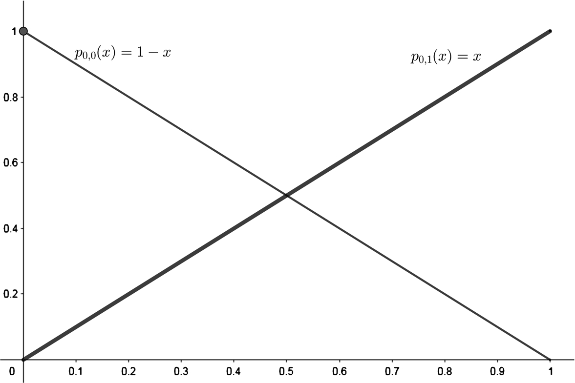
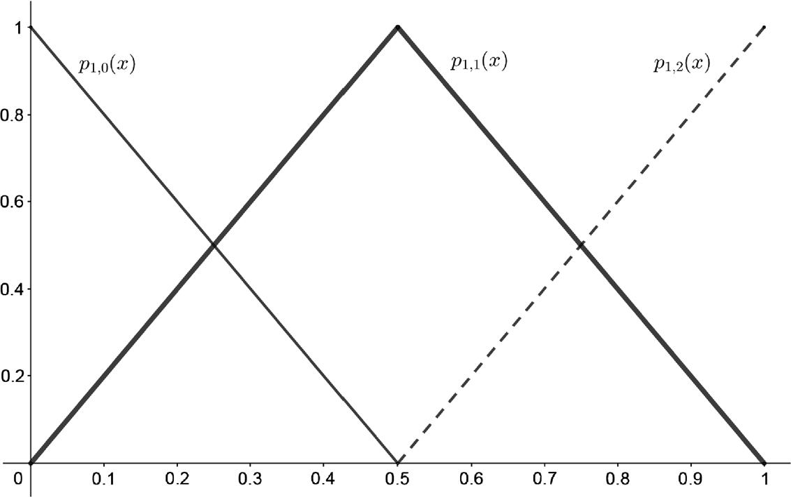
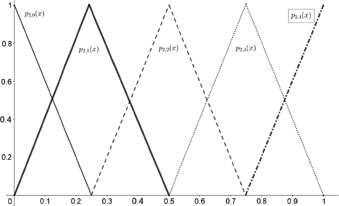
In the case of $C [0, 1]$ , the generating set often used – especially within discussions regarding the Stone–Weierstrass Approximation Theorem – is the set of monomials ${x^{n}}_{n = 0}^{\infty}$ . However, from a computability-theoretic standpoint, this generating set tends to be unwieldy when it comes to the level of control one might like to have in effectively approximating specific functions. Melnikov and Ng made use of, and altered, a more easily-controlled generating set to prove that $C [0, 1]$ is not computably categorical; namely, the set of all continuous piecewise-linear functions defined on the unit interval with finitely many rational breakpoints [12]. In general, as there are many generating sets for a given Banach space, it often is helpful to designate one as “standard.” Below we give the standard generating set of $C [0, 1]$ , which is a slight alteration to the Faber–Schauder system of “tent” functions with maxima at the dyadic rational points (cf. [5]). However, we first define the meet and join of two functions, respectively, as $\begin{array}{l} (f \land g) (x) : = min (f (x), g (x)) = \frac{1}{2} (f (x) + g (x) - | f (x) + g (x) |), \\ (f \lor g) (x) : = max (f (x), g (x)) = \frac{1}{2} (f (x) + g (x) - | f (x) - g (x) |) \end{array}$ (cf. [14]). We will often omit the argument x when writing meets and joins of functions for the sake of space economy.

Definition 2.1.
For a given $f \in C [0, 1]$ , recursively define the double sequence $P_{f} = {p_{i, j} (f)}_{i = 0, j = 0}^{\infty, 2^{i}}$ as follows:
$p_{0, 0} (f) = (1 - f)$ , $p_{0, 1} (f) = f$ ,

For each $i > 0$ and $j ⩽ 2^{i - 1}$ , $\begin{array}{l} p_{i, 2 j} (f) = p_{i - 1, j} (f) - [(p_{i - 1, j} (f) \land p_{i - 1, j + 1} (f)) + (p_{i - 1, j} (f) \land p_{i - 1, j - 1} (f))], \\ p_{i, 2 j + 1} (f) = 2 \cdot (p_{i - 1, j} (f) \land p_{i - 1, j + 1} (f)) . \end{array}$ We will assume $p_{i, j} (f) = 0$ when $j < 0$ or $j > 2^{i - 1}$ .
The standard generating set of $C [0, 1]$ is given by letting f be the identity function, which henceforth we will refer to as $Id$ .

Figures 1, 2, and 3 demonstrate the first several of these “tent” functions generated from $Id$ .

Figure 1.
$p_{0, 0}$ and $p_{0, 1}$ .

Figure 2.
$p_{1, 0}$ , $p_{1, 1}$ , and $p_{1, 2}$ .

Figure 3.
$p_{2, 0}$ , $p_{2, 1}$ , $p_{2, 2}$ , $p_{2, 3}$ , and $p_{2, 4}$ .

To show that the functions defined in Definition 2.1 forms a generating set, we need only note that each member of the Faber–Schauder system for $C [0, 1]$ is included in, or is a linear combination of the functions listed in Definition 2.1. It is well-known that the Faber–Schauder system is linearly dense in $C [0, 1]$ with respect to the supremum norm. It follows readily that the standard generating set described above is linearly dense in $C [0, 1]$ as well. We prove in Section 6 that a generating set for $C [0, 1]$ can be built from any homeomorphism of the unit interval with itself according to the above recipe.

The following theorem is a classical result of analysis that characterizes the isometric isomorphisms between spaces of continuous functions. We will make use of this theorem in Section 6 to prove Proposition 6.1 and subsequently Theorem 1.3.
Theorem 2.2 (Banach–Stone Theorem [6]).

If Q and K are compact metric spaces then for the spaces of real continuous functions $C (Q)$ and $C (K)$ to be isometrically isomorphic it is necessary and sufficient that Q and K be homeomorphic. In this case, an isometric isomorphism T from $C (Q)$ onto $C (K)$ must be given by $\begin{array}{l} T f (t) = h (t) f (ϕ (t)) for t \in K, \end{array}$ where ϕ is a homeomorphism from K onto Q and h is a real-valued unimodular function on K.

2.2. Computable world preliminaries

We assume that the reader is familiar with the notation, terminology, and basic concepts of computability theory as can be found in [16]. Here we cover concepts from computable analysis that are pertinent to the results of this paper. A more expansive treatment of these concepts can be found in [1,15], and [17]. We use the framework for effective metric structure theory of Banach spaces as developed in [4] and [11].

Let $B^{#} = (B, D)$ be a presentation of a Banach space $B$ . $B^{#}$ is a computable presentation of $B$ if there is an algorithm that, given any rational vector f of $ran (D)$ and nonnegative integer k, computes a rational number r so that $| ‖ f ‖ - r | < 2^{- k}$ . In terms of $C [0, 1]$ , it can be shown that the set of all continuous piecewise-linear functions on $[0, 1]$ with finitely many rational breakpoints can be used to form a computable presentation of $C [0, 1]$ ; similarly for the standard generating set $P_{Id}$ as defined in the previous section.

We now define vectors and sequences computable with respect to some computable presentation $B^{#}$ of a Banach space $B$ . We say that a vector $v \in B$ is computable with respect to $B^{#}$ if there is an algorithm that, given nonnegative integer k as input, computes a rational vector u of $B^{#}$ such that $‖ v - u ‖ < 2^{- k}$ . In other words, there is an algorithm that returns arbitrarily good rational vector approximations of $v \in B$ . A sequence ${v_{n}}_{n \in N}$ of vectors in $B$ is said to be computable with respect to $B^{#}$ provided there is an algorithm that, given nonnegative integers n, k as input, produces a rational vector u of $B^{#}$ such that $‖ u - v_{n} ‖ < 2^{- k}$ .

Suppose $B$ is a Banach space with $f \in B$ , and let r be a positive real number. We define the open ball centered at f with radius r (denoted $B (f; r)$ ) to be the set of all vectors $g \in B$ so that $‖ f - g ‖ < r$ . If f is a rational vector of the computable presentation $B^{#}$ of $B$ and $r > 0$ is rational, then we refer to $B (f; r)$ as a rational ball of $B^{#}$ . A code for a rational ball of $B^{#}$ can be obtained from codes for its center and radius.

The next definition will be explicitly referenced in the proof of Theorem 1.2.

Definition 2.3.
Suppose for each $i \in {0, 1}$ that $B_{i}^{#} = (B_{i}, D_{i})$ is a computable presentation of the Banach space $B_{i}$ . A map $T : B_{0} \to B_{1}$ is a computable map of $B_{0}^{#}$ into $B_{1}^{#}$ if there is a computable function P that maps rational balls of $B_{0}^{#}$ to rational balls of $B_{1}^{#}$ such that the following two properties hold.
For rational a ball $b_{1}$ of $B_{0}^{#}$ , $T [b_{1}] \subseteq P (b_{1})$ , whenever $P (b_{1})$ is defined.

Whenever U is a neighborhood of $T (v)$ for $v \in B_{0}$ , there is a rational ball b of $B_{0}^{#}$ such that $v \in b$ and $P (b) \subseteq U$ .

The next theorem, which can be found in [15], will be useful in our proof of Theorem 1.3.
Theorem 2.4.
Suppose for each $i \in {0, 1}$ that $B_{i}^{#} = (B_{i}, D_{i})$ is a computable presentation of the Banach space $B_{i}$ , and that $T : B_{0}^{#} \to B_{1}^{#}$ is bounded and linear. Then, T is computable if and only if T maps a linearly dense computable sequence of $B_{0}^{#}$ to a computable sequence of $B_{1}^{#}$ .

We say that a Banach space $B$ is computably categorical provided that for any two computable presentations $B_{0}^{#}$ and $B_{1}^{#}$ of $B$ there is a computable isometric isomorphism T from $B_{0}^{#}$ onto $B_{1}^{#}$ .

The prior definitions and theorem can all be relativized in the usual way.
3. Overview

Our main results follow a linear progression in the sense that Theorem 1.1 helps us prove Theorem 1.2, which in turn helps us prove Theorem 1.3 and its corollary.

Let $C^{#} = (C [0, 1], D)$ be a computable presentation of $C [0, 1]$ and assume, without loss of generality, that every vector in $ran (D)$ is a unit vector. In Section 4 our chief aim is to develop a $Δ_{2}^{0}$ procedure that searches for a rational vector of $C^{#}$ that is within any desired precision of $1$ . We do this by developing classical criteria that give us the ability to effectively test how “uniformly tall” a unit vector is on the unit interval. Since, with respect to $C^{#}$ , all we can compute is addition, scalar multiplication, and norms of rational vectors of $C^{#}$ , we cannot access any ‘x-value’ information directly. Loosely speaking, what we must do is take advantage of the linear density of $ran (D)$ to find a rational unit vector f of $C^{#}$ that ‘almost’ shares a global max with every other rational unit vector of $C^{#}$ (that is sufficiently close to f). Knowing that unity is $Ø^{'}$ -computable gives us the means by which we can test a rational unit vector v of $C^{#}$ for strict positivity over the unit interval; just use the halting set to compute the result of $‖ 1 - v ‖ < 1$ .

In Section 5 we show that the modulus (or absolute value) operator $| \cdot |$ is $Ø^{″}$ -computable. We know from basic analysis that any unit vector $f \in C [0, 1]$ can be decomposed as $f = f^{+} + f^{-}$ , where $f^{-}$ and $f^{+}$ represent the negative and nonnegative parts of f respectively. As such, $| f | = f^{+} - f^{-}$ . Thus, the key idea for proving Theorem 1.2 comes down to finding a pair of positive rational unit vectors of $C^{#}$ that approximate $f^{+}$ and $f^{-}$ sufficiently well. Notice that $f^{+}$ and $f^{-}$ are disjointly supported vectors; that is, $f^{+} (x) = 0$ for all $x \in [0, 1]$ where $f^{-} (x) \neq 0$ and vice versa. The challenge of finding such vector approximations to $f^{+}$ and $f^{-}$ is ensuring that said approximations are also disjointly supported, or at least ‘almost’ disjointly supported. We handle all of this explicitly in Section 5.

Lastly, in Section 6, we prove Theorem 1.3 and Corollary 1.4. By the definitions of meet and join, as given in Section 2 and by Theorem 1.2, it follows that meets and joins of rational vectors of $C^{#}$ are $Ø^{″}$ -computable. Thus, if we have an X-computable homeomorphism ϕ of the unit interval with itself, the oracle $X \oplus Ø^{″}$ can define $P_{ϕ}$ (cf. Definition 2.1) with respect to any given computable presentation of $C [0, 1]$ . Via the Banach–Stone Theorem mentioned in Section 2, we can then build an $X \oplus Ø^{″}$ -computable map that takes each vector of $P_{Id}$ to its corresponding vector of $P_{ϕ}$ . This map in turn can be extended to an isometric isomorphism. Corollary 1.4 follows immediately from the above.

4. Unity

In this section we begin by providing classical conditions for finding approximations of the constant unit function $1$ , or unity. These will be used to define a search procedure, as outlined in Section 3, which allows the halting set to compute $1$ with respect to any computable presentation of $C [0, 1]$ .

The following definition is at the heart of every proposition that follows.

Definition 4.1.
Let $f, g \in C [0, 1]$ be unit vectors. We define the peak defect of f and g to be $\begin{array}{l} pdef (f, g) = ‖ f ‖ + ‖ g ‖ - ‖ f + g ‖ . \end{array}$

Peak defect, in a sense, is a manner of measuring how far two unit vectors are from sharing global extrema. It is fairly straightforward to see that for unit vectors $f, g \in C [0, 1]$ there is an $x_{0} \in [0, 1]$ such that $f (x_{0}) \cdot g (x_{0}) = 1$ if and only if $pdef (f, g) = 0$ .

We now develop the conditions that, given any $n \in N$ , allow us to search for a rational vector of a computable presentation $C^{#}$ of $C [0, 1]$ that is within $2^{- (n + 1)}$ of the constant unit function $1$ .
Proposition 4.2.
Let $f \in C [0, 1]$ be a unit vector. Then, $| f (x) | > 1 - 2^{- (n + 1)}$ for all $x \in [0, 1]$ if and only if one of the following conditions holds for all unit $g \in C [0, 1]$ :
$‖ f - g ‖ > 2^{- n}$ ,

$pdef (f, g) > 2^{- n}$ ,

$pdef (f, g) < 2^{- (n + 1)}$ .

Proof.
Let f be a unit vector such that $| f (x) | > 1 - 2^{- (n + 1)}$ for all $x \in [0, 1]$ . Suppose g is a unit vector of $C [0, 1]$ . We can suppose that g does not satisfy conditions (1) and (2). Let $c \in [0, 1]$ be such that $| g (c) | = 1$ . Since $‖ f - g ‖ ⩽ 2^{- n}$ , $f (c)$ and $g (c)$ have the same sign. It follows that $\begin{array}{l} | f (c) + g (c) | & ⩽ | f (c) | + | g (c) | \\ < 1 - 2^{- (n + 1)} + 1 . \end{array}$ Therefore, it follows that $\begin{array}{l} pdef (f, g) & = 2 - ‖ f + g ‖ \\ ⩽ 2 - | f (c) + g (c) | \\ < 2^{- (n + 1)} . \end{array}$ We prove the reverse direction by contrapositive. Suppose $| f (x_{0}) | ⩽ 1 - 2^{- (n + 1)}$ for some $x_{0} \in [0, 1]$ . We now define a vector $g \in C [0, 1]$ such that $‖ f - g ‖ ⩽ 2^{- n}$ and $2^{- (n + 1)} ⩽ pdef (f, g) ⩽ 2^{- n}$ . We handle this in two cases.

First suppose, without loss of generality, that $f (x) ⩾ 1 - 2^{- (n + 1)}$ for all $x \in [0, 1]$ . Suppose also that $f (x_{0}) = 1 - 2^{- (n + 1)}$ for some $x_{0} \in [0, 1]$ . Let $\begin{array}{l} g (x) = 2 \cdot (1 - 2^{- (n + 2)}) - f (x) \end{array}$ for all $x \in [0, 1]$ . We claim $‖ g ‖ = 1$ . For, $f (x_{0}) ⩽ f (x)$ for all $x \in [0, 1]$ , which implies $\begin{array}{l} ‖ g ‖ = g (x_{0}) = 2 \cdot (1 - 2^{- (n + 2)}) - (1 - 2^{- (n + 1)}) = 1 . \end{array}$ Therefore g is a unit vector. Furthermore, $| g (x) - f (x) |$ is maximized when $f (x) = 1 - 2^{- (n + 1)}$ ; that is, at $x_{0}$ . Thus, $\begin{array}{l} ‖ f - g ‖ & = 2 \cdot (1 - 2^{- (n + 2)}) - 2 \cdot (1 - 2^{- (n + 1)}) = 2^{- (n + 1)} . \end{array}$ Also, notice that $g (x) + f (x) = 2 \cdot (1 - 2^{- (n + 2)})$ for all $x \in [0, 1]$ , which implies $pdef (f, g) = 2^{- (n + 1)}$ . Thus our requirements for g are satisfied.

Now, suppose there exists an $x_{0} \in [0, 1]$ such that $| f (x_{0}) | < 1 - 2^{- (n + 1)}$ . By continuity, there exists an interval $[a, b]$ so that $| f (a) | = 1 - 2^{- (n + 1)}$ and $\begin{array}{l} 1 - 3 \cdot 2^{- (n + 2)} < | f (x) | < 1 - 2^{- (n + 1)} \end{array}$ for all $x \in (a, b]$ . We will assume without loss of generality that $f (x) > 0$ for all $x \in [a, b)$ . We define g as follows. Set $g (a) = f (a)$ and $g (b) = f (b)$ . Let $c = (a + b) / 2$ and set $g (c) = 1$ . Connect $(a, g (a))$ and $(c, g (c))$ with a line segment; do the same with $(b, g (b))$ and $(c, g (c))$ as well. For all $x \in [0, 1] ∖ [a, b)$ so that $| f (x) | < 1 - 2^{- (n + 1)}$ , set $g (x) = f (x)$ . Lastly, for all $x \in [0, 1] ∖ [a, b)$ so that $| f (x) | ⩾ 1 - 2^{- (n + 1)}$ , set $g (x) = \pm (1 - 2^{- (n + 1)})$ where appropriate so that g is continuous.

We claim $‖ f - g ‖ ⩽ 2^{- n}$ . When $x \in [0, 1] ∖ [a, b)$ so that $| f (x) | ⩾ 1 - 2^{- (n + 1)}$ , $| g (x) | = 1 - 2^{- (n + 1)}$ . Since f attains its maximum value on this set, it follows that $max {| f (x) - g (x) |} = 2^{- (n + 1)}$ when $x \in [0, 1] ∖ [a, b)$ . On $[a, b)$ , $f (x) ⩾ 1 - 2^{- (n + 2)}$ and g attains its maximum value at $(a + b) / 2$ . Therefore $\begin{array}{l} max {| f (x) - g (x) |} < 1 - 1 + 3 \cdot 2^{- (n + 2)} < 2^{- n} . \end{array}$ Lastly, when $x \in [0, 1] ∖ [a, b)$ and $| f (x) | < 1 - 2^{- (n + 1)}$ , $f (x) = g (x)$ . Therefore by all the above it follows that $‖ f - g ‖ ⩽ 2^{- n}$ .

We now claim that $2^{- (n + 1)} ⩽ pdef (f, g) ⩽ 2^{- n}$ . When $x \in [0, 1] ∖ [a, b)$ such that $| f (x) | ⩾ 1 - 2^{- (n + 1)}$ , $| g (x) | = 1 - 2^{- (n + 1)}$ . Since f attains its maximum value on this set, it follows by the definition of g that $max {| f (x) + g (x) |} = 2 - 2^{- (n + 1)}$ . When $x \in [a, b)$ , $1 - 3 \cdot 2^{- (n + 2)} < f (x) ⩽ 1 - 2^{- (n + 1)}$ and g attains its maximum value at $(a + b) / 2$ . Note also that $f (a) + g (a) = 2 (1 - 2^{- (n + 1)}) = 2 - 2^{- n}$ . Therefore $\begin{array}{l} 2 - 2^{- n} ⩽ max {| f (x) + g (x) |} ⩽ 2 - 2^{- (n + 1)} . \end{array}$ Note that when $x \in [0, 1] ∖ [a, b)$ and $| f (x) | < 1 - 2^{- (n + 1)}$ , $\begin{array}{l} ‖ f + g ‖ ⩾ | f (x) + g (x) | ⩾ | 2 f (x) | . \end{array}$ Thus, it follows from the above that $2^{- (n + 1)} ⩽ pdef (f, g) ⩽ 2^{- n}$ . □

Here we demonstrate that the constant unit vector $1$ is $Ø^{'}$ -computable with respect to any computable presentation $C [0, 1]$ by leveraging the conditions found in Proposition 4.2.
Proof of Theorem 1.1.
We begin by defining a procedure P that, on input $m \in N$ , searches for a rational unit vector f of $C^{#}$ so that $| f (x) | ⩾ (1 - 2^{- (m + 1)})$ for all $x \in [0, 1]$ .

First, define S to be the procedure that on input $n \in N$ and nonzero rational vector f of $C^{#}$ searches for a nonzero rational vector g of $C^{#}$ such that $\begin{array}{l} ‖ \frac{f}{‖ f ‖} - \frac{g}{‖ g ‖} ‖ < 2^{- n} and 2^{- (n + 1)} < pdef (\frac{f}{‖ f ‖}, \frac{g}{‖ g ‖}) < 2^{- n}, \end{array}$ and returns g if such a g is found.

Now, suppose we are given an $m \in N$ as input for P. Using oracle $Ø^{'}$ , search for a nonzero rational vector f of $C^{#}$ such that S fails to halt on input m and f, returning $f / ‖ f ‖$ if such an f is found.

Since the set of rational vectors of $C^{#}$ is dense in $C [0, 1]$ we are guaranteed that there is a rational vector f of $C^{#}$ such that $| f | / ‖ f ‖ ⩾ 1 - 2^{- (m + 1)}$ . Thus, by the conditions specified in the proof of Proposition 4.2 and by the density of the rational vectors of $C^{#}$ , for any given $m \in N$ we will indeed find a nonzero rational vector f of $C^{#}$ such that S does not halt on input m and f. Therefore, P is a $Δ_{2}^{0}$ procedure, and it produces a rational vector $f / ‖ f ‖$ such that $| f | / ‖ f ‖ ⩾ 1 - 2^{- (m + 1)}$ .

Now, to compute one of $1$ or $- 1$ , we define two $Ø^{'}$ -computable sequences $S_{0} = {s_{i}^{0}}_{i}$ and $S_{1} = {s_{j}^{1}}_{j}$ such that one of $S_{0}$ or $S_{1}$ converges uniformly to $1$ or $- 1$ .

To this end, we begin by computing a list $R = {r_{k}}_{k ⩾ 3}$ where each $r_{k}$ is the result of running P on input k. Now, we construct $S_{0}$ and $S_{1}$ in stages.
Stage 0

Set $s_{0}^{0} = r_{3}$ and $s_{0}^{1} = 0$ .

Stage $s > 0$

Let $i_{s}$ and $j_{s}$ be the least i and j, respectively, such that $s_{i}^{0}$ and $s_{j}^{1}$ have not been defined. Now, if $‖ r_{s + 3} - r_{3} ‖ > 1$ set $s_{j_{s}}^{1} = r_{s + 3}$ . If $‖ r_{s + 3} - r_{3} ‖ < 1$ set $s_{i_{s}}^{0} = r_{s + 3}$ . Note one of these conditions must occur, for otherwise we have $‖ r_{s + 3} - r_{3} ‖ = 1$ which implies the existence of an $x \in [0, 1]$ such that $| r_{s + 3} (x) | < 1 - 2^{- 3}$ . This is impossible by how we defined the elements of R.

Now, to compute one of either $1$ or $- 1$ up to precision $2^{- n}$ , return $s_{n}^{0}$ if it is defined. Otherwise, return $s_{n}^{1}$ .

By how we constructed our sequences $S_{0}$ and $S_{1}$ , which was done by sorting the $r_{k}$ sequence elements, one of $S_{0}$ or $S_{1}$ must be an infinite sequence. Suppose without loss of generality this sequence is $S_{0}$ and that $s_{0}^{0} > 0$ . We claim that $S_{0}$ converges uniformly to $1$ . Since $s_{0}^{0} > 0$ , by definition $S_{0}$ is a sequence of unit vectors that are all greater than 0. Recall that for all $k ⩾ 3$ , $| r_{k} | ⩾ 1 - 2^{- k}$ . Recall also that, in the above, we defined for each $k > 0$ , $s_{k}^{0} = r_{k^{'}}$ for some $k^{'} > k$ . Thus, let $k \in N$ be given and note that for some $k^{'} > k$ , $\begin{array}{l} s_{k}^{0} = r_{k^{'}} ⩾ 1 - 2^{- k^{'}} > 1 - 2^{- k} . \end{array}$ Since the $r_{k}$ are unit vectors, it follows that $S_{0}$ converges uniformly to $1$ .

Note that since P is $Ø^{'}$ -computable, it follows by the above procedure that $1$ is also $Ø^{'}$ -computable. □

Note that since $1$ is $Ø^{'}$ -computable with respect to any computable presentation $C^{#}$ of $C [0, 1]$ , we can use the halting set to determine whether or not a rational vector f of $C^{#}$ is strictly positive. This can be done by checking the condition $‖ 1 - f / ‖ f ‖ ‖ < 1$ . This will prove useful in the next section.
5. Modulus

Here we first demonstrate that the modulus operator $| \cdot |$ is $Ø^{″}$ -computable with respect to any computable presentation $C^{#}$ of $C [0, 1]$ . We then show that meets and joins are also $Ø^{″}$ -computable with respect to $C^{#}$ . This then gives us a means of proving Theorem 1.3 in Section 6.

Naturally, we can decompose any vector f in $C [0, 1]$ into two disjointly supported vectors $f^{-}$ , and $f^{+}$ , representing the negative and nonnegative parts of f, respectively. Having this decomposition in hand allows us to easily reconstruct $| f |$ from its constituent parts. However, from an effective standpoint, given a computable presentation $C^{#}$ of $C [0, 1]$ , we might not be able to find rational vectors computable with respect to $C^{#}$ that both approximate the negative and nonnegative parts of f and are “perfectly” disjointly supported. Hence, we settle for an approximation of disjointness of support.

Definition 5.1.
Let $f, g \in C [0, 1]$ and let $ϵ > 0$ . f and g are said to be ϵ-almost disjointly supported if $| g (x) | < ϵ$ whenever $| f (x) | > ϵ$ and $| f (x) | < ϵ$ whenever $| g (x) | > ϵ$ .

The following proposition gives us a means by which we can determine if two positive unit vectors are ϵ-almost disjointly supported.
Proposition 5.2.
Let $f, g \in C [0, 1]$ be strictly positive unit vectors and let $ϵ > 0$ . If for all nonnegative h such that $‖ 1 - (f - h) ‖ > 0$ and $‖ f - h ‖ > ϵ$ we have $\begin{array}{l} pdef (\frac{f - h}{‖ f - h ‖}, g) > 1 - ϵ, \end{array}$ then f, g are ϵ-almost disjointly supported.
Proof.
We prove this by contraposition. Suppose f, g are not ϵ-almost disjointly supported. Then there is a point $x_{0} \in [0, 1]$ such that $f (x_{0}), g (x_{0}) ⩾ ϵ$ . It then follows that $h (x_{0}) ⩾ ϵ$ , where $h = f \land g$ . Let $x_{1} \in [0, 1]$ be where $f \land g$ achieves a global maximum. Let $h^{'} = f - h$ . Then since $h ⩾ 0$ it follows that $h^{'} ⩽ f$ as well. Note that $h / ‖ h ‖ = (f - h^{'}) / ‖ f - h^{'} ‖$ attains a global maximum at $x_{1}$ . Since $g (x_{1}) ⩾ ϵ$ , $\begin{array}{l} pdef (\frac{h}{‖ h ‖}, g) & ⩽ 2 - | \frac{h}{‖ h ‖} (x_{1}) + g (x_{1}) | \\ ⩽ 1 - g (x_{1}) \\ ⩽ 1 - ϵ . \end{array}$ Thus we have shown f, g must be ϵ-almost disjointly supported. □

The next proposition indicates how we can use two strictly positive $2^{- k}$ -almost disjointly supported vectors, whose difference approximates $f \in C [0, 1]$ , to approximate $| f |$ . We will make use of these conditions in the proof of Theorem 1.2.
Proposition 5.3.
Let $f, g, h \in C [0, 1]$ be unit vectors so that g, h are nonnegative, $2^{- k}$ -almost disjointly supported for some $k \in N$ , and $‖ f - (g - h) ‖ < 2^{- k}$ . Then, $‖ | f | - (g + h) ‖ ⩽ 2^{- k + 2}$ .
Proof.
Note first that $\begin{array}{l} ‖ | f | - (g + h) ‖ & = ‖ f^{+} + f^{-} - (g + h) ‖ \\ ⩽ ‖ f^{+} - g ‖ + ‖ f^{-} - h ‖ . \end{array}$ We show that $‖ f^{+} - g ‖ ⩽ 2^{- k + 1}$ and note that $‖ f^{-} - h ‖$ follows analogously. Here, we denote the support of a vector $f \in C [0, 1]$ as $supp (f)$ . Now, let $\begin{array}{l} D_{1} = supp (f^{+}) \cap G^{+}, \\ D_{2} = supp (f^{+}) \cap G^{-}, \\ D_{3} = supp (f^{-}) \cap G^{+}, \\ D_{4} = supp (f^{-}) \cap G^{-} \end{array}$ where $G^{+} = {x \in [0, 1] : g (x) > 2^{- k}}$ , $G^{-} = [0, 1] ∖ G^{+}$ . Note that $‖ f^{+} - g ‖$ is equal to the maximum value of ${{max}_{x \in D_{j}} (| f^{+} - g | (x))}_{j = 1, \dots, 4}$ . We show that ${max}_{x \in D_{j}} (| f^{+} - g | (x)) ⩽ 2^{- k + 1}$ for each j.

First, note that on $D_{1}$ , $\begin{array}{l} | f^{+} - (g - h) | = | f - (g - h) | ⩽ ‖ f - (g - h) ‖ < 2^{- k} . \end{array}$ It then follows that for all $x \in D_{1}$ , $- 2^{- k} - h (x) < f^{+} - g (x) < 2^{- k} - h (x)$ . Thus, $| f^{+} (x) - g (x) | < 2^{- k + 1}$ for each $x \in D_{1}$ . By the $2^{- k}$ -almost disjointness of support of g and h, $\begin{array}{l} max_{x \in D_{1}} (| f^{+} - g |) < 2^{- k + 1} . \end{array}$

Note that on $D_{2}$ , $\begin{array}{l} | f^{+} - g + h | ⩽ ‖ f - g + h ‖ < 2^{- k} . \end{array}$ Since $0 < g (x) ⩽ 2^{- k}$ for any $x \in D_{2}$ , this implies $\begin{array}{l} - 2^{- k + 1} ⩽ f^{+} (x) + h (x) ⩽ 2^{- k + 1} \end{array}$ for all $x \in D_{2}$ . We have that $f^{+}, h > 0$ so from the above $0 < h (x) ⩽ 2^{- k + 1}$ . Thus, for all $x \in D_{2}$ , $\begin{array}{l} - 2^{- k} ⩽ f^{+} (x) - g (x) ⩽ 2^{- k + 1} \end{array}$ which implies $\begin{array}{l} max_{x \in D_{2}} (| f^{+} - g | (x)) ⩽ 2^{- k + 1} . \end{array}$

On $D_{3}$ , notice $\begin{array}{l} | - f^{-} - g + h | ⩽ ‖ f - g + h ‖ < 2^{- k} . \end{array}$ Since g and h are $2^{- k}$ -almost disjointly supported, this implies for all $x \in D_{3}$ $\begin{array}{l} - 2^{- k} < f^{-} (x) + g (x) < 2^{- k} + h (x) < 2^{- k + 1} . \end{array}$ Since $f^{-}, g > 0$ on $D_{3}$ we have from the above $\begin{array}{l} 0 < g (x) < f^{-} (x) + g (x) < 2^{- k + 1} . \end{array}$ Since $f^{+} = 0$ on $D_{3}$ , it follows that $\begin{array}{l} max_{x \in D_{3}} (| f^{+} - g | (x)) < 2^{- k + 1} . \end{array}$

Lastly, on $D_{4}$ we have $g ⩽ 2^{- k}$ and $f^{+} = 0$ . It follows immediately that $\begin{array}{l} max_{x \in D_{4}} (| f^{+} - g | (x)) ⩽ 2^{- k} . \end{array}$ Therefore, from the above arguments we can conclude that $‖ f^{+} - g ‖ ⩽ 2^{- k + 1}$ . □

We are now ready to prove Theorem 1.2.
Proof of Theorem 1.2.
In light of Propositions 5.2 and 5.3 we prove $| \cdot | : C [0, 1] \to C [0, 1]$ is $Ø^{″}$ -computable by defining a $Δ_{3}^{0}$ procedure P that maps rational balls $B (f, q)$ of $C^{#}$ to rational balls of $C^{#}$ so that the properties of Definition 2.3 are met. We define P as follows.

First define S to be a procedure that, on input $k \in N$ and rational vectors $f_{0}$ , $f_{1}$ of $C^{#}$ , searches for a nonnegative rational vector h of $C^{#}$ such that the following conditions hold:
$‖ f_{0} - h ‖ > 2^{- k}$ ,

$‖ 1 - (f_{0} - h) ‖ > 0$ ,

$pdef (\frac{f_{0} - h}{‖ f_{0} - h ‖}, f_{1}) ⩽ 1 - 2^{- k}$
and then returns h if found.

Now, compute the least $k_{0} \in N$ such that $q < 2^{- k_{0}}$ . Using $Ø^{″}$ , search for a pair of positive rational unit vectors $f^{+}$ , $f^{-}$ of $C^{#}$ such that $‖ 1 - f^{\pm} ‖ > 0$ , $‖ f - (f^{+} - f^{-}) ‖ < 2^{- k_{0}}$ , and such that S does not halt on inputs $k_{0}$ , $f^{+}$ , $f^{-}$ . If no such vector is found, return $B (w, 2^{- k_{0} + 3})$ where $w = f^{+} + f^{-}$ .

Note that the conditions found in procedure S require the use of the halting set (particularly, to determine whether properties (2) and (3) hold). Furthermore, S may not halt on inputs $k_{0}$ , $f^{+}$ , $f^{-}$ . Thus it follows that procedure P is $Δ_{3}^{0}$ .

Now note by the density of the rational vectors of $C^{#}$ and by Propositions 5.2 and 5.3 we are guaranteed to find positive rational unit vectors $f^{+}$ , $f^{-}$ such that on inputs $k_{0}$ , $f^{+}$ , $f^{-}$ S fails to halt. It follows by Proposition 5.2 that $‖ | f | - w ‖ < 2^{- k_{0} + 3}$ . From this and by how we defined P, property (1) of Definition 2.3 immediately follows.

To show that (2) of Definition 2.3 holds, let $v \in C [0, 1]$ and let U be a neighborhood of $| v |$ . Then let $B (| v |, 2^{- k}) \subseteq U$ . Let f be a rational vector of $C^{#}$ such that $‖ f - v ‖ < 2^{- (k + 2)}$ . We claim $P (b) \subseteq B (| v |, 2^{- k})$ where $b = B (f, q)$ and $2^{- (k + 6)} < q < 2^{- (k + 5)}$ . Note $P (b) = B (w, 2^{- (k + 2)})$ for some rational vector w of $C^{#}$ . By Proposition 5.2, $‖ w - | f | ‖ < 2^{- (k + 2)}$ . Then, by the triangle inequality, $\begin{array}{l} ‖ v - f ‖ & ⩾ ‖ | v | - | f | ‖ \\ ⩾ ‖ (| v | - w) - (| f | - w) ‖ \\ ⩾ ‖ | v | - w ‖ - ‖ | f | - w ‖ \end{array}$ which implies, by Proposition 5.2, that $\begin{array}{l} ‖ | v | - w ‖ ⩽ ‖ v - f ‖ + ‖ | f | - w ‖ < 2^{- (k + 2)} + 2^{- (k + 2)} = 2^{- (k + 1)} . \end{array}$ Thus, if $g \in B (w, 2^{- (k + 2)})$ , we note that the above and the triangle inequality imply $\begin{array}{l} ‖ | v | - g ‖ ⩽ ‖ | v | - w ‖ + ‖ w - g ‖ < 2^{- (k + 1)} + 2^{- (k + 2)} < 2^{- k} . \end{array}$ Therefore $B (w, 2^{- (k + 2)}) \subseteq B (| v |, 2^{- k})$ and property (2) of Definition 2.3 is satisfied. □

The result above combined with the definitions of meets and joins of vectors in $C [0, 1]$ gives us the following. Corollary 5.4.
Let $C^{#}$ be a computable presentation of $C [0, 1]$ . Then, the binary operations ∧ and ∨ are $Ø^{″}$ -computable with respect to $C^{#}$ .
Proof.
This follows immediately from the definition of ∧ and ∨ and Theorem 1.2. □

6. Categoricity

In this section, we prove Theorem 1.3 and Corollary 1.4 by leveraging Corollary 5.4 and the following proposition, whose proof relies upon the Banach–Stone characterization of the isometric isomorphisms of $C [0, 1]$ with itself (cf. Theorem 2.2).

Proposition 6.1.
Let $f \in C [0, 1]$ be a homeomorphism of $[0, 1]$ with itself. Then, the linear span of $P_{f}$ as in Definition 2.1 is dense in $C [0, 1]$ with respect to the supremum norm.
Proof.
Define a surjective linear isometry T from $C [0, 1]$ onto $C [0, 1]$ as $\begin{array}{l} T (g) = g \circ f for all g \in C [0, 1] . \end{array}$ Notice that $T (Id) = f$ and so for all i, j as in Definition 2.1 $\begin{array}{l} T (p_{i, j} (Id; x)) = p_{i, j} (T (Id); x) = p_{i, j} (f; x) \end{array}$ for all $x \in [0, 1]$ . Thus T maps the vectors in $P_{Id}$ injectively onto those of $P_{f}$ . Since $P_{Id}$ is uniformly dense in $C [0, 1]$ , it follows by the Banach–Stone theorem that $P_{f}$ is uniformly dense in $C [0, 1]$ as well. □

The following lemma, which is a corollary of the above, will be helpful in the proof of Theorem 1.3.
Lemma 6.2.
Let f, g be homeomorphisms of $[0, 1]$ with itself, and suppose that $P_{f} = {p_{i, j} (f)}_{i = 0, j = 0}^{\infty, 2^{i}}$ and $P_{g} = {p_{i, j} (g)}_{i = 0, j = 0}^{\infty, 2^{i}}$ are generating sets for $C [0, 1]$ constructed from g and f respectively as in Definition 2.1 . Let $T : C [0, 1] \to C [0, 1]$ be the map defined so that $T (p_{i, j} (f)) = p_{i, j} (g)$ for all i, j. Then, T extends to an isometric endomorphism T of $C [0, 1]$ .

The proof of the above can be easily adapted from that of Proposition 6.1.

We are ready to prove Theorem 1.3.
Proof of Theorem 1.3.
Use $X \oplus Ø^{″}$ to compute a homeomorphism of the unit interval with itself ϕ with respect to $C^{#}$ . Then, it follows from Corollary 5.4 that $X \oplus Ø^{″}$ computes the generating set $P = {p_{i, j} (ϕ)}_{i = 0, j = 0}^{\infty, 2^{i}}$ as explicated in Definition 2.1. Letting ${c_{i, j}}_{i = 0, j = 0}^{\infty, 2^{i}}$ be the standard generating set of $C [0, 1]$ , we have from Lemma 6.2 that the identity map T taking $c_{i, j} \mapsto p_{i, j} (ϕ)$ for all $i \in N$ , $j ⩽ 2^{i}$ extends to an isometric isomorphism from $C [0, 1]$ onto $C^{#}$ . Call this isometric isomorphism T as well. Furthermore, since T maps a linearly dense $X \oplus Ø^{″}$ -computable sequence to an $X \oplus Ø^{″}$ -computable sequence, it follows that T is an $X \oplus Ø^{″}$ -computable isometric isomorphism by relativization of Theorem 2.4. □

It is easy to see that Corollary 1.4 follows immediately from Theorem 1.3.
7. Conclusions

In summary, we have shown that computing unity with respect to any computable presentation $C^{#}$ of $C [0, 1]$ is no more difficult than computing the halting set. Furthermore, we have demonstrated that the modulus operator is $Ø^{″}$ -computable with respect to $C^{#}$ and, as a corollary, proved that meets and joins of rational vectors of $C^{#}$ are also $Ø^{″}$ -computable. In turn, we have shown that if an oracle X computes a homeomorphism of the unit interval with itself with respect to $C^{#}$ , then $X \oplus Ø^{″}$ computes an isometric isomorphism from the standard computable presentation of $C [0, 1]$ onto $C^{#}$ . This then gives us a categoricity result for the restricted class of computable presentations of $C [0, 1]$ as described in Corollary 1.4. The former two theorems by no means directly access ‘x-value’ information of any vector in the space, as we have been working effectively in the signature of Banach spaces. That is, what we accomplished with respect to these results relied only upon ‘y-value’ (i.e. ‘maximum height’) information, and whatever ‘x-value’ information could be garnered from the linear density of a computable presentation of $C [0, 1]$ . The inability to access the ‘x-value’ information of vectors in $C [0, 1]$ likely puts severe limitations what else can be done from an effective standpoint. The following questions come as a natural result of this apparent limitation.

Question 7.1.

What other common operations on vectors in the Banach space $C [0, 1]$ are arithmetical?

Question 7.2.

Is there an arithmetical Turing degree d that computes a homeomorphism with respect to any given computable presentation of the Banach space $C [0, 1]$ ?

If such a degree d can be determined, then much more information can likely be gathered by d regarding the overall shape of graphs of functions in $C [0, 1]$ .

Footnotes

Acknowledgements

I thank Timothy McNicholl and Diego Rojas for many inspiring conversations. I also thank the former, in addition to the anonymous reviewer, for suggestions that improved the composition of the paper.

References

C.J.

Ash and

Knight, Computable Structures and the Hyperarithmetical Hierarchy, Studies in Logic and the Foundations of Mathematics, Vol. 144, North-Holland Publishing Co., Amsterdam, 2000.

Brown, Computable structure theory on Banach spaces, Graduate theses and dissertations, Iowa State University, 2019.

Brown and

T.H.

McNicholl, Analytic computable structure theory and

ℓ^{p}

-spaces part 2, Arch. Math. Logic 59 (2020), 427–443. doi:10.1007/s00153-019-00697-4.

Clanin,

McNicholl and

Stull, Analytic computable structure theory and

ℓ^{p}

-spaces, Fundamenta Mathematicae. 244 (2019), 255–285. doi:10.4064/fm448-5-2018.

M.P.H.

Fabian,

Hájek,

Montesinos and

Zizler, Banach Space Theory, the Basis for Linear and Nonlinear Analysis, CMS Books in Mathematics, 2011.

R.J.

Fleming and

J.E.

Jamison, Isometries on Banach Spaces: Function Spaces, Monographs and Surveys in Pure and Applied Mathematics, CRC Press, 2002.

E.B.

Fokina,

Harizanov and

A.G.

Melnikov, Computable model theory, in: Turing’s Legacy: Developments from Turing’s Ideas in Logic,

Downey, ed., Cambridge University Press, Cambridge, 2014.

E.B.

Fokina,

Kalimullin and

Miller, Degrees of categoricity of computable structures, Archive for Mathematical Logic 49(1) (2009), 51–67. doi:10.1007/s00153-009-0160-4.

Fröhlich and

J.C.

Shepherdson, Effective procedures in field theory, Philosophical Transactions of the Royal Society of London. Series A. Mathematical and Physical Sciences 248 (1956), 407–432.

10.

D.R.

Hirschfeldt,

Kramer,

Miller and

Shlapentokh, Categoricity properties for computable algebraic fields, Transactions of the American Mathematical Society 367(6) (2015), 3981–4017. doi:10.1090/S0002-9947-2014-06094-7.

11.

T.H.

McNicholl, Computable copies of

ℓ^{p}

, Computability 6(4) (2017), 391–408. doi:10.3233/COM-160065.

12.

A.G.

Melnikov and

K.M.

Ng, Computable structures and operations on the space of continuous functions, Fundamenta Mathematicae 233(2) (2014), 1–41.

13.

A.G.

Melnikov and

Nies, The classification problem for compact computable metric spaces, in: The Nature of Computation, Lecture Notes in Comput. Sci., Vol. 7921, Springer, Heidelberg, 2013, pp. 320–328.

14.

Pilar and

Mendoza, Banach Spaces of Vector-Valued Functions, Lecture Notes in Mathematics, Vol. 1676, Springer-Verlag, Berlin, 1997. MR 1489231.

15.

M.B.

Pour-El and

Richards, Computability in Analysis and Physics, Perspectives in Mathematical Logic, Springer Verlag, Berlin, New York, 1989.

16.

Soare, Turing Computability Theory and Applications, Springer, Berlin, Heidelberg, 2016.

17.

Weihrauch, Computable Analysis: An Introduction, Texts in Theoretical Computer Science, Springer, Berlin, New York, 2000.