Effective aspects of Hausdorff and Fourier dimension

Abstract

In this paper, we study Hausdorff and Fourier dimension from the point of view of effective descriptive set theory and Type-2 Theory of Effectivity. Working in the hyperspace $K (X)$ of compact subsets of X, with $X = {[0, 1]}^{d}$ or $X = R^{d}$ , we characterize the complexity of the family of sets having sufficiently large Hausdorff or Fourier dimension. This, in turn, allows us to show that family of all the closed Salem sets is $Π_{3}^{0}$ -complete. One of our main tools is a careful analysis of the effectiveness of a classical theorem of Kaufman. We furthermore compute the Weihrauch degree of the functions computing Hausdorff and Fourier dimension of closed sets.

Keywords

Computable analysis Hausdorff dimension Fourier dimension Salem sets

1. Introduction

Hausdorff dimension is probably the most important and well studied among the notions of fractal dimensions, and it plays a central role in analysis and geometric measure theory. In recent work, Jack and Neil Lutz [31] proved a point-to-set principle linking the (classical) Hausdorff dimension of a set with the (relative) effective Hausdorff dimension of its points. If we restrict our attention to singletons, we can characterize the effective Hausdorff dimension of ${ξ}$ by means of the Kolmogorov complexity of ξ [32], which establishes a surprising connection between two (apparently) very distant notions.

A powerful tool to study the Hausdorff dimension of Borel subsets of $R^{d}$ is provided by the Fourier transform. Indeed, Frostman’s lemma draws an interesting connection between the Hausdorff dimension of a set and the decay of the Fourier transform of a (probability) measure supported on it. This leads to the notion of Fourier dimension. It is known that the Fourier dimension of a Borel set cannot exceed its Hausdorff dimension.

This work is part of a long-term effort, involving many researchers, aimed at exploring the recursion-theoretic properties of the Fourier dimension. While no point-to-set principles can hold for the Fourier dimension (in such a generality), analyzing the complexity of the Fourier dimension in simpler cases can shed light on the general behavior of the Fourier dimension itself (up to now, still not deeply understood).

Salem sets arise naturally when combining geometric measure theory and harmonic analysis. A set $A \subset R^{d}$ is called Salem iff ${dim}_{H} (A) = {dim}_{F} (A)$ , where ${dim}_{H}$ and ${dim}_{F}$ denote the Hausdorff and the Fourier dimension respectively. Explicit (i.e. non-random) Salem sets are not easy to build. A classic example comes from the theory of Diophantine approximation of real numbers: for every $α ⩾ 0$ , the set $E (α)$ of α-well approximable numbers is Salem with dimension $2 / (2 + α)$ . The computation of its Hausdorff dimension is due to Jarník [26] and Besicovitch [3], while the result on its Fourier dimension is due to Kaufman [27]. The reader is referred to [4] or [49] for detailed proofs of Kaufman’s theorem. The construction presented in [49] will play a central role in the rest of this work.

As a consequence of a result of Gatesoupe [20], subsets of $R^{d}$ obtained by the rotation of a 1-dimensional Salem sets with dimension α (having at least two points) are Salem of dimension $d - 1 + α$ , and this provides a simple way for building Salem sets of dimension at least $d - 1$ in $R^{d}$ .

Explicit examples of non-Salem sets are the symmetric Cantor sets with dissection ratio $1 / n$ for $n > 2$ : they are known to have null Fourier dimension and Hausdorff dimension $log (2) / log (n)$ (see [34, Sec. 4.10] and [35, Thm. 8.1]). Every subset of a n-dimensional hyperplane is a 0-Fourier dimensional subset of $R^{d}$ when $n < d$ , while it can have any Hausdorff dimension up to n.

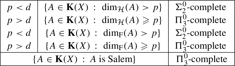
In recent work [33], we studied the complexity, from the point of view of classical descriptive set theory, of a number of relations involving the Hausdorff and the Fourier dimension. In particular, we studied the conditions ${dim}_{H} (A) > p$ , ${dim}_{F} (A) > p$ , ${dim}_{H} (A) ⩾ p$ , ${dim}_{F} (A) ⩾ p$ , “A is Salem”, when $p \in R$ and A is a closed subset of $[0, 1]$ , ${[0, 1]}^{d}$ , and $R^{d}$ . In particular, we proved that having Hausdorff/Fourier dimension $> p$ and $⩾ p$ are, respectively, a ${\underset{\sim}{Σ}}_{2}^{0}$ -complete and a ${\underset{\sim}{Π}}_{3}^{0}$ -complete conditions. Similarly, we showed that the family of Salem sets is ${\underset{\sim}{Π}}_{3}^{0}$ -complete. In this paper we explore the same conditions from the point of view of effective descriptive set theory and Type-2 Theory of Effectivity (TTE). Notice that in [23] the authors showed that the sets of elements of the Cantor space having (respectively) effective Hausdorff dimension $> α$ and $⩾ α$ , where α is a $Δ_{2}^{0}$ -computable real, are (respectively) $Σ_{2}^{0}$ and $Π_{3}^{0}$ .

The paper is organized as follows. After briefly introducing the relevant background notions (Section 2), we present some results on the lightface structure of the hyperspaces of closed and compact sets (Section 3) and on computable measure theory (Section 4) that will be needed for the main results. In particular, we show that the hyperspace of compact subsets of a computably compact space is computably compact (Lemma 3.5), the hyperspace of closed subsets of the Euclidean space is computably compact (Proposition 3.6) and that the space of probability measures on a computably compact space is computably compact (Theorem 4.1). Section 5 is devoted to the proof of an effective version of the above mentioned theorem by Kaufman, stated in Theorem 5.6. Section 6 contains the main results on the effective complexity of the conditions mentioned above, and can be summarized as follows: if $X = {[0, 1]}^{d}$ or $X = R^{d}$ then,

where $K (X)$ is the hyperspace of compact subsets of X (endowed with the canonical lightface structure induced by the Hausdorff metric, introduced in Section 3). The complexities remain the same if we consider the hyperspace of closed sets. In particular, the fact that the family of closed Salem subsets of $[0, 1]$ is $Π_{3}^{0}$ -complete answers a question asked by Slaman during the IMS Graduate Summer School in Logic, held in Singapore in 2018. In Section 7, we use our results to characterize the Weihrauch degree of the maps computing the Hausdorff and the Fourier dimension of a closed set, in particular answering a question raised by Fouché ([9]) and Pauly.

2. Background

Throughout the paper, we will use $B (x, r)$ to denote the open ball with center x and radius r. We also fix a computable enumeration ${(q_{i})}_{i \in N}$ of $Q^{+}$ .

2.1. Hausdorff and Fourier dimension

Let us briefly introduce the relevant notions from geometric measure theory. For a more thorough presentation the reader is referred to [18].

Let $(X, d)$ be a separable metric space and let $A \subset X$ . We denote the diameter of A by $diam (A)$ . For every $s ⩾ 0$ , $δ \in (0, + \infty]$ we define $\begin{array}{l} H_{δ}^{s} (A) : = inf {\sum_{i \in I} diam {(E_{i})}^{s} : {E_{i}}_{i \in I} is a δ -cover of A}, \\ H^{s} (A) : = lim_{δ \to 0^{+}} H_{δ}^{s} (A) = sup_{δ > 0} H_{δ}^{s} (A), \end{array}$ where ${E_{i}}_{i \in I}$ is a δ-cover of A if $A \subset ⋃_{i \in I} E_{i}$ and $diam (E_{i}) ⩽ δ$ for each $i \in I$ . The function $H^{s}$ is called s-dimensional Hausdorff measure. The Hausdorff dimension of A is defined as $\begin{matrix} {dim}_{H} (A) : = sup {s \in [0, + \infty) : H^{s} (A) > 0} . \end{matrix}$

It is well-known that, as a consequence of Frostman’s lemma (see [34, Thm. 8.8]), the Hausdorff dimension of a Borel subset of $R^{d}$ can be equivalently written as $\begin{matrix} sup {s \in [0, d] : (\exists μ \in P (A)) (\exists c > 0) (\forall x \in R^{d}) (\forall r > 0) (μ (B (x, r)) ⩽ c r^{s})}, \end{matrix}$ where $P (A)$ is the set of Borel probability measures supported on A (in other words, for Borel sets Hausdorff and capacitary dimensions coincide).

This characterization suggests the possibility to use the tools of harmonic analysis to obtain estimates on the Hausdorff dimension. We can define the Fourier transform of a probability measure $μ \in P (R^{d})$ as the function $\begin{matrix} \hat{μ} : R^{d} \to C : = x \mapsto \int_{R^{d}} e^{- i ξ \cdot x} d μ (x) \end{matrix}$ where $ξ \cdot x$ denotes scalar product. The Fourier dimension of $A \subset R^{d}$ is then defined as $\begin{matrix} {dim}_{F} (A) : = sup {s \in [0, d] : (\exists μ \in P (A)) (\exists c > 0) (\forall x \in R^{d}) (| \hat{μ} (x) | ⩽ c | x |^{- s / 2})} . \end{matrix}$

It is known that, for every Borel $A \subset R^{d}$ , ${dim}_{F} (A) ⩽ {dim}_{H} (A)$ (see [34, Chap. 12]). If ${dim}_{F} (A) = {dim}_{H} (A)$ then A is called Salem set. We denote the collection of Salem subsets of $X \subset R^{d}$ with $S (X)$ .

For background notions on the Fourier transform the reader is referred to [46]. For its applications to geometric measure theory see [35].

We notice that the Hausdorff dimension is countably stable:

for every family ${A_{i}}_{i \in N}$ , ${dim}_{H} (⋃_{i} A_{i}) = {sup}_{i} {dim}_{H} (A_{i})$ [34, p. 59];

invariant under bi-Lipschitz maps:

for every α-Hölder continuous map $f : R^{n} \to R^{m}$ we have ${dim}_{H} (f (A)) ⩽ α^{- 1} {dim}_{H} (A)$ [18, Prop. 3.3].

In particular, the inclusion map

ι : R^{n} \to R^{m}

, with

n ⩽ m

, preserves the Hausdorff dimension.

None of the above properties hold, in full generality, for the Fourier dimension. In fact, it is not even finitely stable [16, Sec. 1.3] and does not behave well under Hölder continuous transformations [17, Sec. 8]. Moreover, it is sensitive to the choice of the ambient space: as mentioned, every $A \subset R^{n}$ has null Fourier dimension when seen as a subset of $R^{m}$ with $n < m$ . However, some regularity properties hold if we restrict our attention to special cases. We mention, in particular, that the Fourier dimension is inner regular for compact sets, i.e. $\begin{matrix} {dim}_{F} (A) = sup {{dim}_{F} (K) : K \subset A and K is compact}, \end{matrix}$ and countably stable for closed sets [16, Prop. 5], i.e. for every countable family ${A_{k}}_{k}$ of closed subsets of $R^{d}$ we have $\begin{matrix} {dim}_{F} (⋃_{k} A_{k}) = sup_{k} {dim}_{F} (A_{k}) . \end{matrix}$ Moreover, the Fourier dimension is invariant under similarities or affine (invertible) transformations (this is a simple consequence of the properties of the Fourier transform).

2.2. Computability on represented spaces

In this paper, we use the standard approach of Type-2 Theory of Effectivity (TTE) to define a notion of computability on a wide range of spaces. We now introduce the main definitions, for a more detailed presentation the reader is referred to [38,48].

Let $N^{N}$ be the Baire space and let $N^{< N}$ be the set of finite sequences of natural numbers. Let also $2^{N}$ be the Cantor space and $2^{< N}$ be the set of finite binary sequences. Both $N^{N}$ and $2^{N}$ are endowed with the usual product topology. We sometimes describe a string by a list of its elements. E.g. we write $(n_{0}, n_{1}, \dots, n_{k})$ for the string $σ : = i \mapsto n_{i}$ . Similarly, we can describe an infinite string by $(n_{0}, n_{1}, \dots)$ , when it is clear from the context how to continue the sequence. We write $()$ for the empty sequence. We write $| σ |$ for the length of σ and $σ ⌢ τ$ for the concatenation of the strings σ and τ. We will use the symbol $⟨ \cdot ⟩$ to denote a fixed computable bijection $N^{< N} \to N$ with computable inverse. It is often convenient to write $⟨ n_{0}, \dots, n_{k} ⟩$ in place of $⟨ (n_{0}, \dots, n_{k}) ⟩$ . In the literature, the symbol $⟨ \cdot ⟩$ is often used to denote also the join between two (of the same length, finite or infinite) strings. With a (relatively) small abuse of notation, if x, y are two strings of the same length we will write1

¹
The exact details of the definition of the join are often not relevant. E.g. a common way to define the join of $x, y \in N^{N}$ is letting $⟨ x, y ⟩ (2 n) : = x (n)$ and $⟨ x, y ⟩ (2 n + 1) : = y (n)$ .

⟨ x, y ⟩ (i) : = ⟨ x (i), y (i) ⟩

and

⟨ x_{0}, x_{1}, \dots ⟩ (⟨ i, j ⟩) : = x_{i} (j)

A represented space is a pair $(X, δ_{X})$ where X is a set and $δ_{X} : \subseteq N^{N} \to X$ is a partial surjection called representation map. For every $x \in X$ , the elements of $δ_{X}^{- 1} (x)$ are called $δ_{X}$ -names for x (we just say names if there is no ambiguity on the representation map).

We can exploit the classical notion of computability on $N^{N}$ (see [48] for an introduction) to induce a notion of computability on any represented space: let f be a partial multi-valued function between the represented spaces $(X, δ_{X})$ and $(Y, δ_{Y})$ (in symbols $f : \subseteq X ⇉ Y$ ). A realizer for f is a partial function $F : \subseteq N^{N} \to N^{N}$ such that, for every $p \in dom (f \circ δ_{X})$ , we have that $δ_{Y} (F (p)) \in f (δ_{X} (p))$ . We say that f is $(δ_{X}, δ_{Y})$ -computable if it has a computable realizer (again, we just say computable if the representation maps are clear from the context). We say that f is realizer-continuous if it has a continuous realizer. The set of realizer-continuous partial functions between represented spaces is a represented space itself ([48, Sec. 2.3]).

As the notation suggests, the induced notion of computability is intrinsically tied to the choice of the representation maps. If δ and $δ^{'}$ are two representation maps for X, we say that δ is (topologically) reducible to $δ^{'}$ , and we write $δ ⩽ δ^{'}$ (resp. $δ ⩽_{t} δ^{'}$ ), if there is a (continuous) computable map $F : \subseteq N^{N} \to N^{N}$ s.t. $δ (p) = δ^{'} (F (p))$ for every $p \in dom (δ)$ . The maps δ and $δ^{'}$ are called (topologically) equivalent, written $δ \equiv δ^{'}$ (resp. $δ \equiv_{t} δ^{'}$ ), if $δ ⩽ δ^{'}$ and $δ^{'} ⩽ δ$ (resp. $δ ⩽_{t} δ^{'}$ and $δ^{'} ⩽_{t} δ$ ).

Often times, spaces are naturally endowed with some canonical topology, and it would be desirable that the topological structure agrees with the computational one, i.e. that the notions of continuity and realizer-continuity agree. We will consider (and mainly focus our attention on) the so-called admissible representations, which intuitively are those that satisfy this requirement.

Definition 2.1 ([43, Def. 1]).

Let $(X, τ_{X})$ be a topological space. A representation map $δ_{X}$ of X is called admissible w.r.t. $τ_{X}$ if it is continuous and, for every other continuous representation map δ on X, we have $δ ⩽_{t} δ_{X}$ .

In other words, an admissible representation of X is $⩽_{t}$ -maximal among the continuous representation of X. We will just say that a representation is admissible if there is no ambiguity on the topology.

Theorem 2.2 ([48, Thm. 3.2.11]).

Let $(X, δ_{X}, τ_{X})$ , $(Y, δ_{Y}, τ_{Y})$ be admissibly represented second-countable $T_{0}$ spaces. For every $f : \subseteq X \to Y$ , $\begin{matrix} f is continuous ⟺ f is realizer-continuous . \end{matrix}$

In particular, whenever X and Y are admissibly represented, the space $C_{}^{} (X, Y)$ of continuous functions from X to Y is a represented space.

Clearly, the very existence of an admissible representation for the topological space $(X, τ_{X})$ depends on the topology itself: a family $B$ of subsets of X is called a pseudobase iff for every open set $U \subset X$ , every $x \in U$ and every sequence ${(y_{n})}_{n \in N}$ converging to x, $\begin{matrix} (\exists B \in B) (\exists n_{0} \in N) ({x} \cup {y_{n} : n ⩾ n_{0}} \subset B \subset U) . \end{matrix}$

Theorem 2.3 ([43, Thm. 13]).

A topological space $(X, τ_{X})$ admits an admissible representation $δ_{X}$ iff it is $T_{0}$ and admits a countable pseudobase.

2.3. Representations on (hyper)spaces

While (the proof of) Theorem 2.3 provides an explicit definition of an admissible representation for a wide variety of spaces, in many practical situations this is not the representation map we endow our space with. Observe that, while all admissible representation maps are topologically equivalent, they do not necessarily induce the same notions of computability, i.e. they may not be (computably) equivalent.

Let $X = (X, d, α)$ be a separable metric space, where $d : X \times X \to R$ is the distance function and $α : N \to X$ is an enumeration of a dense subset of X. The Cauchy representation on X is the map $δ_{C} : \subseteq N^{N} \to X$ defined as $\begin{matrix} δ_{C} (p) = x : ⟺ lim_{n \to \infty} α (p (n)) = x, \end{matrix}$ where $dom (δ_{C}) : = {p \in N^{N} : (\forall n) (\forall m > n) (| α (p (n)) - α (p (m)) | ⩽ 2^{- n})}$ is the set of rapidly converging sequences. The Cauchy representation is the “canonical” representation map for separable metric spaces. It is equivalent to the representation map that names $x \in X$ via any $q \in N^{N}$ s.t. ${x} = ⋂_{n \in N} B (α (q (n)), 2^{- n})$ .

Recall that ${(q_{i})}_{i \in N}$ is a canonical computable enumeration of the rationals. We say that X is a computable metric space if the set $\begin{matrix} {(i, j, n, m) \in N^{4} : q_{i} < d (α (n), α (m)) < q_{j}} \end{matrix}$ is computably enumerable, i.e. if the restriction of the distance function to $ran {(α)}^{2}$ is computable. We can always assume that, if X is infinite, α is an injective map (i.e. every element of the dense subset of X has a unique index). Indeed, for every infinite computable metric space $(X, d, α)$ there is an injective subsequence β of α s.t. the spaces $(X, d, α)$ and $(X, d, β)$ are computably homeomorphic (i.e. there is a computable bijection with computable inverse) [21, Thm. 2.9].

Let $(Y, τ_{Y})$ be a second-countable topological space. We say that $(Y, {(B_{n})}_{n \in N})$ is an effective (topological) space if ${(B_{n})}_{n \in N}$ is an enumeration of a basis for $τ_{Y}$ s.t. there is a computable function $φ : N^{< N} \times N \to N$ s.t. $\begin{matrix} ⋂_{i < | σ |} B_{σ (i)} = ⋃_{k \in N} B_{φ (σ, k)} . \end{matrix}$ Every effective topological space $(Y, {(B_{n})}_{n \in N})$ can be endowed with the structure of represented space by defining an (admissible) representation map $δ_{Y}$ that names a point $y \in Y$ via an enumeration of the set ${i : y \in B_{i}}$ . Notice that a computable metric space $(X, d, α)$ can be seen as an effective space by considering the “standard” enumeration of the basis for X (i.e. $B_{⟨ i, j ⟩} = B (α (i), q_{j})$ ). In this case, the Cauchy representation on X is equivalent to the representation $δ_{X}$ .

For every topological space Z, the family of Borel subsets of Z can be stratified in a hierarchy, called the Borel hierarchy. The levels of this hierarchy are defined by transfinite recursion on $1 ⩽ ξ < ω_{1}$ , where $ω_{1}$ is the first uncountable ordinal. We denote by ${\underset{\sim}{Σ}}_{1}^{0} (Z)$ and ${\underset{\sim}{Π}}_{1}^{0} (Z)$ respectively the family of the open and the closed subsets of Z. For every $ξ > 1$ we define:

${\underset{\sim}{Σ}}_{ξ}^{0} (Z) : = {⋃_{n} A_{n} ∖ B_{n} : A_{n}, B_{n} \in {\underset{\sim}{Σ}}_{ξ_{n}}^{0} (Z), ξ_{n} < ξ, n \in N}$ ,

${\underset{\sim}{Π}}_{ξ}^{0} (Z) : = {X ∖ A : A \in {\underset{\sim}{Σ}}_{ξ}^{0} (Z)}$ .

Moreover, for every ξ, we define

{\underset{\sim}{Δ}}_{ξ}^{0} (Z) : = {\underset{\sim}{Σ}}_{ξ}^{0} (Z) \cap {\underset{\sim}{Π}}_{ξ}^{0} (Z)

. In particular,

{\underset{\sim}{Δ}}_{1}^{0} (Z)

is the family of clopen subsets of Y. The families

{\underset{\sim}{Σ}}_{2}^{0} (Z)

and

{\underset{\sim}{Π}}_{2}^{0} (Z)

are often written resp.

F_{σ} (Z)

and

G_{δ} (Z)

. It is known that

\underset{\sim}{B} (Z) = ⋃_{ξ} {\underset{\sim}{Σ}}_{ξ}^{0} (Z) = ⋃_{ξ} {\underset{\sim}{Π}}_{ξ}^{0} (Z) = ⋃_{ξ} {\underset{\sim}{Δ}}_{ξ}^{0} (Z)

, where

\underset{\sim}{B} (Z)

denotes the family of Borel subsets of Z. We will omit the dependency from the space if there is no ambiguity.

For metric spaces (in fact, for Hausdorff spaces), the definition of the pointclass ${\underset{\sim}{Σ}}_{ξ}^{0}$ can be simplified letting $\begin{matrix} {\underset{\sim}{Σ}}_{ξ}^{0} = {⋃_{n} A_{n} : A_{n} \in {\underset{\sim}{Π}}_{ξ_{n}}^{0}, ξ_{n} < ξ, n \in N} . \end{matrix}$

Let W and Z be topological spaces and let $A \subset W$ , $B \subset Z$ . We say that A is Wadge reducible to B if there is a continuous function $f : W \to Z$ s.t. $\begin{matrix} x \in A ⟺ f (x) \in B . \end{matrix}$

Let $\underset{\sim}{Γ}$ be a Borel class and assume that Z is Polish. We say that B is $\underset{\sim}{Γ}$ -hard if $A ⩽_{W} B$ for every $A \in \underset{\sim}{Γ} (N^{N})$ . If B is $\underset{\sim}{Γ}$ -hard and $B \in \underset{\sim}{Γ} (Z)$ then we say that B is $\underset{\sim}{Γ}$ -complete.

For every effective second-countable space $(Y, {(B_{n})}_{n \in N})$ , we say that $A \subset Y$ is effectively open if $A = ⋃_{n \in N} B_{φ (n)}$ for some computable function $φ : N \to N$ . The set of effectively open subsets of Y is denoted by $Σ_{1}^{0} (Y)$ . In other words, an effective open set is a computable union of basic open sets. The complement of an effectively open set is called effectively closed and the family of all effectively closed subsets of Y is denoted by $Π_{1}^{0} (Y)$ .

Notice that $Σ_{1}^{0} (Y)$ sets can be indexed using the code for a computable function defining them. In other words, there is a canonical indexing ${(A_{i})}_{i \in N}$ of the $Σ_{1}^{0} (Y)$ sets. This allows us to define

$Σ_{2}^{0} (Y) : = {A \subset Y : A = ⋃_{n \in N} A_{φ (2 n + 1)} ∖ A_{φ (2 n)}, for some computable φ}$ ;

$Π_{2}^{0} (Y) : = {Y ∖ A : A \in Σ_{2}^{0} (Y)}$ .

We can inductively define the (Kleene’s) arithmetical hierarchy, also called lightface hierarchy, by letting

{(A_{i}^{n})}_{i \in N}

be an effective indexing of the

Σ_{n}^{0} (Y)

sets and defining

$Σ_{n + 1}^{0} (Y) : = {A \subset Y : A = ⋃_{i \in N} A_{φ (2 n + 1)}^{n} ∖ A_{φ (2 n)}^{n}, for some computable φ}$ ;

$Π_{n + 1}^{0} (Y) : = {Y ∖ A : A \in Σ_{n + 1}^{0} (Y)}$ .

The lightface hierarchy can be relativized in a straightforward manner, by defining, for

z \in 2^{N}

\begin{matrix} Σ_{1}^{0, z} (Y) : = {A \subset Y : A = ⋃_{n \in N} B_{f (n)} for some z -computable function f}, \end{matrix}

and then, define the classes

Π_{n}^{0, z}

Σ_{n + 1}^{0, z}

Δ_{n}^{0, z}

accordingly. It is important to mention that the lightface classes are universal for their corresponding boldface ones. Formally, if Γ is a lightface class among

Σ_{n}^{0}

Π_{n}^{0}

and

\underset{\sim}{Γ}

is the corresponding boldface pointclass, then

\begin{matrix} P \in \underset{\sim}{Γ} (Y) ⟺ (\exists z \in N^{N}) (P \in Γ^{z} (Y)), \end{matrix}

see e.g. [36, Thm. 3E.4].

For every effective space $(Y, {(B_{n})}_{n \in N})$ and every $k ⩾ 1$ , we can define the represented spaces $({\underset{\sim}{Σ}}_{k}^{0}, δ_{{\underset{\sim}{Σ}}_{k}^{0}})$ , $({\underset{\sim}{Π}}_{k}^{0}, δ_{{\underset{\sim}{Π}}_{k}^{0}})$ , $({\underset{\sim}{Δ}}_{k}^{0}, δ_{{\underset{\sim}{Δ}}_{k}^{0}})$ inductively by:

$δ_{{\underset{\sim}{Σ}}_{1}^{0}} (p) : = ⋃_{i \in ran (p)} B_{i}$ ;

$δ_{{\underset{\sim}{Π}}_{k}^{0}} (p) : = Y ∖ δ_{{\underset{\sim}{Σ}}_{k}^{0}} (p)$ ;

$δ_{{\underset{\sim}{Σ}}_{k + 1}^{0}} (⟨ p_{0}, q_{0}, p_{1}, q_{1}, \dots ⟩) : = ⋃_{i \in N} δ_{{\underset{\sim}{Σ}}_{k}^{0}} (p_{i}) ∖ δ_{{\underset{\sim}{Σ}}_{k}^{0}} (q_{i})$ ;

$δ_{{\underset{\sim}{Δ}}_{k}^{0}} (⟨ p, q ⟩) : = δ_{{\underset{\sim}{Σ}}_{k}^{0}} (p)$ , iff $p, q \in dom (δ_{{\underset{\sim}{Σ}}_{k}^{0}})$ and $δ_{{\underset{\sim}{Σ}}_{k}^{0}} (p) = Y ∖ δ_{{\underset{\sim}{Σ}}_{k}^{0}} (q)$ .

We notice that the $Σ_{k}^{0}$ sets are exactly those having a computable $δ_{{\underset{\sim}{Σ}}_{k}^{0}}$ -name (and similarly for $Π_{k}^{0}$ , $Δ_{k}^{0}$ ).

If Y and $Y^{'}$ are effective spaces, we say that $A \subset Y^{'}$ is effectively Wadge reducible to $B \subset Y$ , and write $A ⩽_{m} B$ , if there is a recursive functional $f : Y^{'} \to Y$ s.t. $x \in A$ iff $f (x) \in B$ . Let Γ be a lightface pointclass as above and assume that Y is an effective Polish space. We say that B is Γ-hard if $A ⩽_{m} B$ for every $A \in Γ (N^{N})$ . If B is Γ-hard and $B \in Γ (Y)$ then we say that B is Γ-complete. Standard examples2

²
The standard proofs showing that the listed sets are $\underset{\sim}{Γ}$ -complete for their respective class are, in fact, effective. See [28, Sec. 23.A].

of Γ-complete sets are the following:

\begin{matrix} Q_{2} : = {x \in 2^{N} : (\forall^{\infty} m) (x (m) = 0)} & Σ_{2}^{0} -complete, \\ N_{2} : = {x \in 2^{N} : (\exists^{\infty} m) (x (m) = 0)} & Π_{2}^{0} -complete, \\ S_{3} : = {x \in 2^{N \times N} : (\exists k) (\exists^{\infty} m) (x (k, m) = 0)} & Σ_{3}^{0} -complete, \\ P_{3} : = {x \in 2^{N \times N} : (\forall k) (\forall^{\infty} m) (x (k, m) = 0)} & Π_{3}^{0} -complete, \end{matrix}

where

(\exists^{\infty} m)

and

(\forall^{\infty} m)

mean respectively

(\forall n) (\exists m ⩾ n)

and

(\exists n) (\forall m ⩾ n)

While often there is a natural choice for an effective basis, when working with represented spaces we can exploit the representation map to induce a lightface structure in a canonical way.

Let us introduce the Sierpiński space $S : = {0, 1}$ . The space $S$ is endowed with the topology ${\emptyset, {1}, S}$ . This space is represented as follows: the only name for 0 is the string that is constantly 0, while every other string in $N^{N}$ is a name for 1.

We can notice that, if $(X, δ_{X})$ is a represented space and $O (X)$ is the final topology on X induced by $δ_{X}$ , then the open sets $U \in O (X)$ are exactly the subsets of X s.t. the characteristic function $χ_{U} : X \to S$ is realizer-continuous (see also [38, Sec. 4]). In particular, we can represent an open set $U \in O (X)$ using a name for $χ_{U}$ . This, in turn, allows us to represent a closed set (in the final topology on X) via a name for its complement. Using the jumps of the Sierpiński space, we can obtain an analogous characterization for the pointclasses ${\underset{\sim}{Σ}}_{ξ}^{0} (X)$ ([40, Sec. III and Prop. 30], see also [14]).

In other words, using the Sierpiński space, we can define a representation map for the sets ${\underset{\sim}{Σ}}_{k}^{0}$ , ${\underset{\sim}{Π}}_{k}^{0}$ , ${\underset{\sim}{Δ}}_{k}^{0}$ , for any represented space $(X, δ_{X})$ . For separable metric spaces, the two representations are equivalent (see [5,38]).

The same ideas allow us to induce a lightface structure on any represented space. Indeed, for a represented space $(X, δ_{X})$ , we can define the effectively open sets as follows: $\begin{matrix} A \in Σ_{1}^{0} (X) : ⟺ the characteristic function χ_{A} : X \to S of A is computable. \end{matrix}$ The Sierpiński space is, thus, useful to obtain a notion of semi-decidability in represented spaces. For a more detailed discussion the reader is referred to [12,39,40].

3. The hyperspaces of closed and compact sets

The hyperspaces of closed and compact sets will play a crucial role in this paper. The space ${\underset{\sim}{Π}}_{1}^{0} (X)$ of closed subsets of a topological space X is usually endowed with a number of topologies we now recall. For a more thorough presentation, the reader is referred to [2,30].

Let us define $\begin{array}{l} U : = {{F \in {\underset{\sim}{Π}}_{1}^{0} (X) : F \cap C = \emptyset} : C \in {\underset{\sim}{Π}}_{1}^{0} (X)}, \\ L : = {{F \in {\underset{\sim}{Π}}_{1}^{0} (X) : F \cap U \neq \emptyset} : U \in {\underset{\sim}{Σ}}_{1}^{0} (X)} . \end{array}$ The topology $τ_{U V}$ having $U$ as a prebase is called upper topology or upper Vietoris topology, while the topology $τ_{L}$ having $L$ as a prebase is called lower topology or lower Vietoris topology ([30, Def. 1.3.1 and def. 1.3.2]). The Vietoris topology $τ_{V}$ is the topology having as a prebase the family $U \cup L$ .

We also consider the collection $U_{K}$ defined as $\begin{matrix} U_{K} : = {{F \in {\underset{\sim}{Π}}_{1}^{0} (X) : F \cap K = \emptyset} : K \in K (X)}, \end{matrix}$ where $K (X)$ is the family of all compact subsets of X. The family $U_{K}$ is a prebase for the topology $τ_{U F}$ on ${\underset{\sim}{Π}}_{1}^{0} (X)$ called upper Fell topology. We define the Fell topology $τ_{F}$ on ${\underset{\sim}{Π}}_{1}^{0} (X)$ as the topology having as a prebase the set $U_{K} \cup L$ . For this reason, the lower Vietoris topology is also called lower Fell topology.

If we restrict our attention to compact subsets of X, we can define the topological space $K (X) = (K (X), τ_{V} |_{K (X)})$ obtained by endowing the family of compact subsets of X with the topology induced by the Vietoris topology on ${\underset{\sim}{Π}}_{1}^{0} (X)$ . This choice is motivated by the following observation: if X is a metric space with distance d, we can define the Hausdorff metric $d_{H}$ on $K (X)$ as follows: $\begin{matrix} d_{H} (K, L) : = \{\begin{matrix} 0 & if K = L = \emptyset \\ 1 & if exactly one between K and L is \emptyset \\ max {δ (K, L), δ (L, K)} & otherwise \end{matrix} \end{matrix}$ where $δ (K, L) : = {max}_{x \in K} d (x, L) / (1 + d (x, L))$ . It is known that the Hausdorff metric $d_{H}$ is compatible with the Vietoris topology on $K (X)$ ([28, Ex. 4.21]) and that if X is Polish then so is $K (X)$ ([28, Thm. 4.22]).

We notice that $({\underset{\sim}{Π}}_{1}^{0} (X), τ_{V})$ fails to be paracompact, and hence metrizable, if X is not compact ([29, Thm. 2]). The Fell topology is the preferred choice when working with closed sets, since if X is Polish and locally compact then $({\underset{\sim}{Π}}_{1}^{0} (X), τ_{F})$ is a Polish compact space and its Borel space is exactly the Effros-Borel space ([28, Ex. 12.7]). If X is compact then the Fell and the Vietoris topologies coincide, and the same holds for the upper Fell and the upper Vietoris topologies.

In the following, let $(X, d, α)$ be a computable metric space. We already mentioned that the set ${\underset{\sim}{Π}}_{1}^{0} (X)$ can be seen as a represented space, where a name for a closed set is a list of basic open balls that exhaust the complement. This representation map is often3

³
see [7, Def. 3.4], [8, Sec. 2]. In [10] it is introduced in Def. 3.5(1) and is denoted $δ_{union}$ .

denoted

ψ_{-}

, and

ψ_{-}

-names provide negative information on the set they represent. The represented space

({\underset{\sim}{Π}}_{1}^{0} (X), ψ_{-})

is often denoted

A (X)

A_{-} (X)

in the literature.

In contrast, the positive information representation $ψ_{+}$ for closed sets is defined as $\begin{matrix} ψ_{+} (p) = F : ⟺ (\forall n \in N) (n + 1 \in ran (p) ⟺ F \cap B_{n} \neq \emptyset), \end{matrix}$ where ${(B_{n})}_{n \in N}$ is the canonical enumeration of basic open balls of X. In other words, a $ψ_{+}$ -name for F is a list of all the basic open sets that intersect F ([7, Def. 3.1], it is denoted $δ^{<}$ in [10, Def. 3.1(1)]). The elements of the represented space $({\underset{\sim}{Π}}_{1}^{0} (X), ψ_{+})$ are called closed overt sets, and the space is sometimes denoted $V (X)$ in the literature, e.g. [15, Sec. 2].

We denote the join of both positive and negative information representations with ψ. Formally $\begin{matrix} ψ (⟨ p, q ⟩) = F : ⟺ ψ_{-} (p) = ψ_{+} (q) = F . \end{matrix}$ This is denoted $ψ_{=}$ in [7, Def. 3.1] and $δ^{=}$ in [10, Def. 3.1].

It is known that the representation maps $ψ_{-}$ , $ψ_{+}$ , and ψ are admissible respectively for the upper Fell, lower Fell, and Fell topology on ${\underset{\sim}{Π}}_{1}^{0} (X)$ [7, Sec. 3].

We mention the following known facts.

Theorem 3.1 ([7, Sec. 7]).

Let X be a computable metric space. The following operations are computable:

$\cup : ({\underset{\sim}{Π}}_{1}^{0} (X), δ) \times ({\underset{\sim}{Π}}_{1}^{0} (X), δ) \to ({\underset{\sim}{Π}}_{1}^{0} (X), δ) : = (A, B) \mapsto A \cup B$ , for $δ \in {ψ_{-}, ψ_{+}, ψ}$ .

$⋂ : {({\underset{\sim}{Π}}_{1}^{0} (X), ψ_{-})}^{N} \to ({\underset{\sim}{Π}}_{1}^{0} (X), ψ_{-}) : = {(A_{n})}_{n \in N} \mapsto ⋂_{n \in N} A_{n}$ .

Notice however that $\cap : ({\underset{\sim}{Π}}_{1}^{0} (X), ψ) \times ({\underset{\sim}{Π}}_{1}^{0} (X), ψ) \to ({\underset{\sim}{Π}}_{1}^{0} (X), ψ)$ is in general not computable, and not even continuous (see e.g. [28, Ex. 4.29(viii)]). For a more precise analysis of the complexity of the intersection operator see [7, Thm. 7.1].

Let us introduce the following notion:

Definition 3.2.
A compact subset K of a computable metric space $(X, d, α)$ is called co-c.e. compact if $\begin{matrix} {σ \in N^{< N} : K \subset ⋃_{i < | σ |} B_{σ (i)}} \end{matrix}$ is computably enumerable. We say that K is computably compact if it is co-c.e. compact and there exists a computable dense sequence in K.

We say that a sequence ${(K_{n})}_{n \in I}$ is uniformly co-c.e. compact if each $K_{n}$ is co-c.e. compact in a computable metric space $X_{n}$ and the set $\begin{matrix} {(n, σ) \in N \times N^{< N} : K_{n} \subset ⋃_{i < | σ |} B_{σ (i)}^{n}} \end{matrix}$ is computably enumerable, where $B_{k}^{n}$ is the k-th basic open ball in $X_{n}$ . In other words, the sequence ${K_{n}}_{n \in I}$ is uniformly co-c.e. compact if there is a single computable function witnessing that each $K_{n}$ is co-c.e. compact.

The notions of co-c.e. compact and computably compact are standard notions in computable analysis (see e.g. [8, Def. 2.10]). Notice that being co-c.e. compact implies being $Π_{1}^{0} (X)$ and that every $Π_{1}^{0} (X)$ subset of a co-c.e. compact space is co-c.e. compact. Clearly a computable metric space is co-c.e. compact iff it is computably compact. Moreover, if K is co-c.e. compact (resp. computably compact) and $f : K \to Y$ is computable and surjective, then Y is co-c.e. compact (resp. computably compact) as well (see [38, Prop. 5.3]). Several equivalent conditions to being computably compact are listed in [38, Prop. 5.2]. The notions of co-c.e. compact and computably compact can be extended in a straightforward way to effective spaces.

We also mention the following simple lemma:
Lemma 3.3.
If X is co-c.e. compact then so is $X^{N}$ .
Proof.
The fact that the finite product of co-c.e. compact spaces is co-c.e. compact follows from [38, Prop. 5.4]. To prove that $X^{N}$ is co-c.e. compact, recall that an open set in $X^{N}$ is of the type $B : = \prod_{j \in N} B_{j}$ , where each $B_{j}$ is open in X and $B_{j} \neq X$ only for finitely many indexes. Such an open set is canonically represented via (a name for) a finite sequence ${(B_{j})}_{j < N}$ with the understanding that $B_{j} = X$ for every $j ⩾ N$ .

Let ${(B_{i})}_{i < k}$ be a finite sequence of open subsets of $X^{N}$ , where $B_{i}$ is represented by ${(B_{j}^{i})}_{j < N_{i}}$ . This sequence trivially induces a finite sequence ${(C_{i})}_{i < k}$ of open subsets of $X^{N}$ , where $N : = {max}_{i < k} N_{i}$ : for every i and every $j \in {N_{i}, \dots, N - 1}$ , let $B_{j}^{i} : = X$ and define $C_{i} : = \prod_{j < N} B_{j}^{i}$ . The sequence ${(B_{i})}_{i < k}$ covers $X^{N}$ iff ${(C_{i})}_{i < k}$ covers $X^{N}$ . The claim follows from the fact that the sets ${(X^{n})}_{n \in N}$ are uniformly co-c.e. compact. □

Since $K (X) \subset {\underset{\sim}{Π}}_{1}^{0} (X)$ , we can represent the compact subsets of X using the subspace representation induced by the representation we put on ${\underset{\sim}{Π}}_{1}^{0} (X)$ . At the same time, we mentioned that $K (X)$ is compatible with the Hausdorff metric. Letting β be an enumeration of the finite subsets of $ran (α)$ , the space $(K (X), d_{H}, β)$ is a computable metric space (as the finite subsets of $ran (α)$ are a dense subset of $K (X)$ ). In particular, $K (X)$ can be (canonically) endowed with the Cauchy representation $δ_{H}$ induced by $d_{H}$ and β. The Cauchy representation for the hyperspace of non-empty compact subset of the Euclidean space was studied in [11] under the name $δ_{Haus}$ , and then extended to generic computable metric spaces in [10], where the symbol $δ_{Hausdorff}$ was used.

Two additional representations maps for $K (X)$ that are used in the literature (see e.g. [6, Sec. 4]) are the maps $κ_{-}$ and κ: the former names a compact set K via a list of all finite covers of K with basic open balls, while κ-names have the additional requirement that all basic balls in each cover have to intersect K. The compact sets having computable $κ_{-}$ -names (resp. κ-names) are exactly the co-c.e. compact (resp. computably compact) sets. The representation maps $κ_{-}$ and κ have been studied in [10,11] under the names $δ_{cover}$ and $δ_{\min - cover}$ respectively.
Proposition 3.4.
Let X be a co-c.e. compact subspace of the Euclidean space $(R^{d}, | \cdot |, α_{Q^{d}})$ , where $| \cdot |$ is the Euclidean distance and $α_{Q^{d}}$ is an enumeration of $Q^{d}$ . Let $ψ_{-}^{'} : = ψ_{-} |_{ψ_{-}^{- 1} (K (X))}$ be the restriction of $ψ_{-}$ to names of compact subsets of X, and similarly let $ψ^{'} : = ψ |_{ψ^{- 1} (K (X))}$ . The following holds on $K (X)$ :
$κ_{-} \equiv ψ_{-}^{'}$ ;

$κ \equiv ψ^{'} \equiv δ_{H}$ .

Proof.
The equivalence $κ_{-} \equiv ψ_{-}^{'}$ follows from [11, Thm. 4.6]. Precisely, the representation $δ_{K}^{>}$ names a compact set K via a $ψ_{-}^{'}$ -name of K and the index of a ball B s.t. $K \subset \overline{B}$ ([11, Def. 4.1]). If X is compact then the equivalence $ψ_{-}^{'} \equiv δ_{K}^{>}$ is straightforward.

The equivalence $κ \equiv ψ^{'}$ follows from [11, Cor. 4.7] using the fact that $ψ^{'} \equiv δ_{K}^{=}$ for a compact X. Indeed, a $δ_{K}^{=}$ -name of a compact set K is a $ψ^{'}$ -name of K and the index of a ball B s.t. $K \subset \overline{B}$ ([11, Def. 4.1]).

In [11, Thm. 4.10], the Cauchy representation $δ_{Haus}$ (i.e. the restriction of $δ_{H}$ to names of non-empty compact sets) has been proven equivalent to the restriction $δ_{K}^{=} |^{K^{}}$ of $δ_{K}^{=}$ to names of non-empty compact sets. We now explicitly show that $δ_{H} \equiv ψ^{'}$ (i.e. the empty set is not problematic if X is co-c.e. compact).

Recall that for every non-empty closed G, $d_{H} (G, \emptyset) = 1$ . $δ_{H} ⩽ ψ^{'}$ :
As mentioned after the definition of Cauchy representation, we can think of a $δ_{H}$ -name p for F as a list of (indexes for) basic open balls ${(B_{n})}_{n \in N}$ w.r.t. the Hausdorff metric s.t. all the balls contain F and the radius of $B_{n}$ is $2^{- n}$ . Since the empty set is isolated in $K (X)$ , it is enough to consider $n > 1$ . Indeed, without loss of generality we can assume that we can computably tell whether $B_{n}$ is centered on ∅ (e.g. we can assume that the empty set has a unique index in the list of dense subsets of $K (X)$ ). If $B_{n}$ is centered on ∅ then $F = \emptyset$ (as $B_{n} = {\emptyset}$ ). Otherwise $F \neq \emptyset$ , and we can use $δ_{Haus} ⩽ δ_{K}^{=} |^{K^{}}$ and $δ_{K}^{=} ⩽ ψ^{'}$ .
$ψ^{'} ⩽ δ_{H}$ :
Let $⟨ p, q ⟩$ be a $ψ^{'}$ -name for F, where p is a negative information name and q is a positive information name for F. If $F = \emptyset$ then p is a list of basic open balls that cover X. On the other hand, if $F \neq \emptyset$ then q eventually lists some basic open ball (in X) that intersects F (q is allowed not to produce any information at a given stage). In other words, we wait for some sufficiently large n so that either $⋃_{i < n} B_{p (i)}$ covers X or q commits to some open ball at stage n. This allows us to determine whether F is empty or not. If $F = \emptyset$ we can trivially compute a sequence of basic open balls (in $K (X)$ ) centered on ∅ with rapidly decreasing radii. Otherwise, as in the previous reduction, we can use $ψ^{'} ⩽ δ_{K}^{=}$ and $δ_{K}^{=} |^{K^{}} ⩽ δ_{Haus}$ to produce a $δ_{H}$ -name for F.
□

For the sake of readability, we adopt the following notation:

$F_{U} (X) = ({\underset{\sim}{Π}}_{1}^{0} (X), τ_{U F}, ψ_{-})$ is the hyperspace of closed subsets of X, endowed with the upper Fell topology and the negative representation $ψ_{-}$ ;

$F (X) = ({\underset{\sim}{Π}}_{1}^{0} (X), τ_{F}, ψ)$ is the hyperspace of closed subsets of X, endowed with the Fell topology and the full representation ψ;

$K_{U} (X) = (K (X), τ_{U F} |_{K (X)}, ψ_{-}^{'})$ is the hyperspace of compact subsets of X, endowed with the upper Fell topology and the negative representation restricted to names of compact sets, i.e. $ψ_{-}^{'} = ψ_{-} |_{ψ_{-}^{- 1} (K (X))}$ ;

$K (X) = (K (X), τ_{V} |_{K (X)}, ψ^{'})$ is the hyperspace of compact subsets of X, endowed with the Vietoris topology and the full representation restricted to names of compact sets, i.e. $ψ^{'} = ψ |_{ψ^{- 1} (K (X))}$ .

The following lemma is the effective counterpart of [28, Thm. 4.26].
Lemma 3.5.
If $(X, d, α)$ is computably compact then so is* $K (X)$ .
Proof.
Recall that a basic open ball in $K (X)$ is a set of the type $B_{⟨ n, m ⟩} = {K \in K (X) : d_{H} (K, β (n)) < q_{m}}$ , where β is the fixed enumeration of the finite subsets of $ran (α)$ and ${(q_{i})}_{i \in N}$ is the canonical enumeration of $Q^{+}$ . In particular, if $β (n) = {b_{0}, \dots, b_{k - 1}}$ then $\begin{matrix} B_{⟨ n, m ⟩} = {K \in K (X) : K \subset ⋃_{i < k} B (b_{i}, q_{m}) \land (\forall i < k) (K \cap B (b_{i}, q_{m}) \neq \emptyset)} . \end{matrix}$

Let ${(B_{i} = B_{⟨ n_{i}, m_{i} ⟩})}_{i < k}$ be a finite sequence of basic open balls in $K (X)$ . We want to describe a c.e. procedure to check whether ${(B_{i})}_{i < k}$ covers $K (X)$ . For the sake of readability, let us define $r (i) : = q_{m_{i}}$ and $D_{i} : = ⋃_{b \in β (n_{i})} B (b, r (i))$ for every $i < k$ . We first check if $r (i) > 1$ for some $i < k$ (any ball with radius $> 1$ covers $K (X)$ , and in this case we can give a positive answer) or if there is $j < k$ s.t. $β (n_{j}) = \emptyset$ (recall that the empty set is isolated, and a ball with radius $⩽ 1$ covers ∅ iff it is centered on it, hence if such a j is missing we give a negative answer). Since these two conditions are computable, to prove the result it is enough to show that there is a c.e. procedure to determine if a finite sequence ${(B_{i})}_{i < k}$ with $r (i) ⩽ 1$ and $β (n_{i}) \neq \emptyset$ for all $i < k$ covers $K (X) ∖ {\emptyset}$ .

We now define a c.e. subtree T of ${(N \times ran (α))}^{⩽ k}$ (where k is the length of the fixed finite sequence of basic open balls) where each string $σ \in T$ is labeled with a compact subset $Y_{σ}$ of X. A string $σ = ((a_{0}, b_{0}), \dots, (a_{h - 1}, b_{h - 1}))$ is in T iff $\begin{matrix} h ⩽ k \land (\forall i < h) (a_{i} < k \land b_{i} \in β (n_{a_{i}})) \land (\forall i, j < h, i \neq j) (a_{i} \neq a_{j}) \land Y_{σ [h - 1]} \subset D_{a_{h - 1}}, \end{matrix}$ where $σ [h - 1]$ denotes the prefix of σ of length $h - 1$ . The string σ is labeled with $Y_{σ} : = X ∖ ⋃_{i < h} B (b_{i}, r (a_{i}))$ .

Notice that, since X is computably compact, then so are all the sets $Y_{σ}$ . In fact, they are uniformly computably compact: given a finite sequence ${(B_{i})}_{i < n}$ of open balls, we can compute the index of a computable functional witnessing that $Y : = X ∖ ⋃_{i < n} B_{i}$ is computably compact. This follows from $\begin{matrix} Y \subset ⋃_{j < | τ |} B_{τ (j)} ⟺ X \subset ⋃_{i < n} B_{i} \cup ⋃_{j < | τ |} B_{τ (j)} . \end{matrix}$ In particular, this shows that the condition $Y_{σ [h - 1]} \subset D_{a_{h - 1}}$ (and hence $σ \in T$ ) is computably enumerable.

We claim that $\begin{matrix} {(B_{i})}_{i < k} covers K (X) ∖ {\emptyset} ⟺ for each leaf σ \in T, Y_{σ} = \emptyset . \end{matrix}$ This implies the computable compactness of $K (X)$ , as the condition on the right is computably enumerable ( $Y_{σ} = \emptyset$ is equivalent to $Y_{σ}$ being covered by the empty set and the quantification on σ is bounded because T is computably finitely branching).

For the right-to-left direction, assume that there is a non-empty $K \in K (X) ∖ ⋃_{i < k} B_{i}$ . We show that there is a leaf σ s.t. $Y_{σ} \neq \emptyset$ . We proceed iteratively as follows, defining a list of sequences $σ_{s}$ s.t. $K \subset Y_{σ_{s}}$ : let $σ_{- 1} : = ()$ . At stage $s < k$ , we look for some unmarked (i.e. not selected in any previous stage) $a_{s} < k$ s.t. $Y_{σ_{s - 1}} \subset D_{a_{s}}$ . If such a choice is possible then, since $K \notin B_{a_{s}}$ and $K \subset D_{a_{s}}$ , there is $b_{s} \in β (n_{a_{s}})$ s.t. $K \cap B (b_{s}, r (a_{s})) = \emptyset$ . In particular, $K \subset Y_{σ_{s - 1}} ∖ B (b_{s}, r (a_{s}))$ , hence letting $σ_{s} : = σ_{s - 1} ⌢ ((a_{s}, b_{s}))$ , we have $K \subset Y_{σ_{s}}$ , which implies that $Y_{σ_{s}} \neq \emptyset$ . We then mark $a_{s}$ as visited and go to the next stage. If there is no $a_{s} < k$ that satisfies the requirements then $σ : = σ_{s - 1}$ is a leaf for T but $Y_{σ} \neq \emptyset$ (as $K \subset Y_{σ}$ ). Notice that looking for some unmarked $a_{s}$ guarantees that no choice of $a_{s}$ is possible at stage $k + 1$ .

Let us now prove the left-to-right implication. Assume that $σ = ((a_{0}, b_{0}), \dots, (a_{h - 1}, b_{h - 1}))$ is a leaf for T. Notice that, for each $j < h$ and each $K \in K (X) ∖ {\emptyset}$ , if $K \in B_{a_{j}}$ then for every $b \in β (n_{a_{j}})$ , $K \cap B (b, r (a_{j})) \neq \emptyset$ , and hence $K ⊄ Y_{σ [j + 1]}$ . In particular, if $Y_{σ} \neq \emptyset$ then, for every $j < h$ , $Y_{σ} \notin B_{a_{j}}$ . Moreover, since σ is a leaf, there is no pair $(a, b)$ s.t. $Y_{σ} \subset D_{a}$ , which implies that $Y_{σ} \notin ⋃_{i < k} B_{i}$ . □
Proposition 3.6.
$F (R^{d})$ is computably compact.
Proof.
We show that there is a computable surjection $f : K ({[0, 1]}^{d}) \to F (R^{d})$ , and the claim will follow using Lemma 3.5 and the remarks following Definition 3.2. Fix a computable homeomorphism $φ : {(0, 1)}^{d} \to R^{d}$ and define $\begin{matrix} f (K) : = φ (K \cap {(0, 1)}^{d}) . \end{matrix}$ It is easy to see that, for $K \in K ({[0, 1]}^{d})$ , $f (K)$ is closed. Moreover, f is surjective: for every $F \in {\underset{\sim}{Π}}_{1}^{0} (R^{d})$ , $φ^{- 1} (F)$ is closed in the relative topology of ${(0, 1)}^{d}$ . If we denote with G its closure w.r.t. the relative topology of ${[0, 1]}^{d}$ , we have that $G ∖ φ^{- 1} (F) \subset \partial ({[0, 1]}^{d})$ , hence, in particular, $f (G) = F$ .

Finally, we show that f is computable. Recall that both $K ({[0, 1]}^{d})$ and $F (R^{d})$ are admissibly represented with the full information representation. Let $⟨ p, q ⟩ \in N^{N}$ be a name for $K \in K ({[0, 1]}^{d})$ . To compute a negative information name for $f (K)$ from p, notice that, since $φ^{- 1}$ is a computable homeomorphism (and, in particular, it is a total computable surjection), as mentioned in the proof of [6, Prop. 3.7] we have that the map $F_{U} (Y) \to F_{U} (X) : = A \mapsto φ (A)$ . Intuitively: for every basic open $B \subset {[0, 1]}^{d} ∖ K$ we can computably list a sequence of basic open balls of $R^{d}$ exhausting $φ (B)$ . On the other hand, notice that a basic open ball B of $R^{d}$ intersects $f (K)$ iff there is $i \in N$ s.t. $B_{q (i)} \subset φ^{- 1} (B)$ (this follows from the fact that φ is a homeomorphism). In particular, to produce a positive information name for $f (K)$ , we list $B_{n} \subset R^{d}$ whenever we find some i s.t. $B_{q (i)} \subset φ^{- 1} (B_{n})$ (which is a computable condition). □

Recall that, if X is not compact, then the hyperspace $({\underset{\sim}{Π}}_{1}^{0} (X), τ_{V})$ of closed subsets X endowed with the Vietoris topology is not metrizable. We now show that it is not even admissibly represented.
Proposition 3.7.
Let $F_{U V} (X) = ({\underset{\sim}{Π}}_{1}^{0} (X), τ_{U V})$ denote the hyperspace of closed subsets of X endowed with the upper Vietoris topology $τ_{U V}$ . The space $F_{U V} (R)$ (and hence $F_{U V} (R^{d})$ ) does not have a countable pseudobase. In particular, it is not second-countable and it is not admissibly represented.
Proof.
Fix a countable sequence ${P_{i}}_{i \in N}$ of subsets of $F_{U V} (R)$ . To show that ${P_{i}}_{i \in N}$ is not a pseudobase we build a closed set F and an open set $U$ which contains F s.t. for every i, either $F \notin P_{i}$ or $P_{i} ⊄ U$ . We define $F : = {x_{i} : i \in N}$ , where ${(x_{i})}_{i \in N}$ is a strictly increasing sequence iteratively defined as follows: for each i, let $n_{i}$ be the smallest integer greater than $x_{j} + 1$ for every $j < i$ (if $i = 0$ we let $n_{i} : = 0$ ). Choose an unbounded $P_{i} \in P_{i}$ . If there is none we just define $x_{i} : = n_{i}$ . Let $y_{i} \in P_{i} \cap [n_{i}, \infty)$ and choose $x_{i}$ s.t. $x_{i} > y_{i} + 1$ . In particular $d (y_{i}, {x_{j}}_{j ⩽ i}) > 1$ .

Notice that, for every $i \neq j$ , $d (x_{i}, x_{j}) > 1$ , hence the sequence ${(x_{i})}_{i \in N}$ does not have accumulation points. In particular, the set $F : = {x_{i} : i \in N}$ is closed and unbounded. Fix ε sufficiently small, e.g. $ε = 1 / 4$ , and define the open set $F_{ε} : = {x \in R : d (x, F) < ε}$ and $U : = {G \in {\underset{\sim}{Π}}_{1}^{0} (R) : G \subset F_{ε}}$ .

The open set $U$ and the closed set F witness the fact that ${P_{i}}_{i \in N}$ is not a pseudobase. Indeed, for every i, either every $P \in P_{i}$ is bounded (and hence $F \notin P_{i}$ ), or the set $P_{i}$ defined above witnesses that $P_{i} ⊄ U$ (as by construction $d (y_{i}, F) > 1$ ).

This implies also that $F_{U V} (R)$ is not second-countable, as every base is a pseudobase. The fact that it is not admissibly represented follows by Theorem 2.3. The claim generalizes to $F_{U V} (R^{d})$ as every pseudobase of $F_{U V} (R^{d})$ induces a pseudobase on $F_{U V} (R)$ by projection. □
Corollary 3.8.
The space $({\underset{\sim}{Π}}_{1}^{0} (R), τ_{V})$ (and hence $({\underset{\sim}{Π}}_{1}^{0} (R^{d}), τ_{V})$ ) does not have a countable pseudobase. In particular, it is not second-countable and it is not admissibly represented.
Proof.
This follows from the proof of Proposition 3.7. Indeed, the above proof only uses a closed set $F \in {\underset{\sim}{Π}}_{1}^{0} (R)$ and an open set $U \subset F_{U V} (R)$ to show that no countable subfamily of ${\underset{\sim}{Π}}_{1}^{0} (R)$ is a pseudobase. Since the upper Vietoris topology is coarser than the Vietoris topology, the same argument applies to $({\underset{\sim}{Π}}_{1}^{0} (R), τ_{V})$ . The claim would not follow immediately if, in the proof of Proposition 3.7 we would have exploited a convergent sequence to F, as convergence is a weaker notion in the upper Vietoris topology. □

We conclude this section with the effective counterpart of [1, Lem. 1.3]:
Lemma 3.9.
Let X, Y be computable metric spaces. If Y is co-c.e. compact then, for every $F \in Π_{1}^{0} (X \times Y)$ , ${proj}_{X} F \in Π_{1}^{0} (X)$ . If $Y = ⋃_{n \in N} Y_{n}$ where the sequence ${(Y_{n})}_{n \in N}$ is uniformly co-c.e. compact, then for every $F \in Σ_{2}^{0} (X \times Y)$ , ${proj}_{X} F \in Σ_{2}^{0} (X)$ .
Proof.
Let us first assume that Y is co-c.e. compact and let $F \in Π_{1}^{0} (X \times Y)$ . Let $p \in N^{N}$ be a computable map s.t. $F^{C} = ⋃_{n \in N} B_{p {(n)}_{0}}^{X} \times B_{p {(n)}_{1}}^{Y}$ . Notice that $B_{n}^{X} \subset {({proj}_{X} F)}^{C}$ iff the preimage $B_{n}^{X} \times Y$ of $B_{n}^{X}$ via the projection map ${proj}_{X}$ is contained in the complement of F.

Let $φ_{p} : N^{< N} \times N \to N$ be a computable function s.t., for all $σ \in N^{< N}$ $\begin{matrix} ⋂_{i \in ran (σ)} B_{p {(i)}_{0}}^{X} = ⋃_{k \in N} B_{φ_{p} (σ, k)}^{X} . \end{matrix}$ Such a map exists because X is a computable metric space (and hence effective second-countable).

To show that ${({proj}_{X} F)}^{C}$ is effectively open, notice that $\begin{matrix} {n \in N : (\exists σ \in N^{< N}) (⋃_{i \in ran (σ)} B_{p {(i)}_{1}}^{Y} = Y and (\exists k) (n = φ_{p} (σ, k)))} \in Σ_{1}^{0} . \end{matrix}$ This follows from the fact that $φ_{p}$ is computable and that $⋃_{i \in ran (σ)} B_{p {(i)}_{1}}^{Y} = Y$ is $Σ_{1}^{0}$ because Y is co-c.e. compact. This shows that we can computably enumerate a list of open sets exhausting the complement of ${proj}_{X} F$ , i.e. ${proj}_{X} F \in Π_{1}^{0} (X)$ .

The same argument shows (still assuming Y co-c.e. compact) that if $D \in Π_{1}^{0} (N \times X \times Y)$ then ${proj}_{N \times X} D \in Π_{1}^{0} (N \times X)$ (it is enough to replace X with $N \times X$ ). If $F \in Σ_{2}^{0} (X \times Y)$ then it can be written as $F = {proj}_{X \times Y} D$ , for some $D \in Π_{1}^{0} (N \times X \times Y)$ . In particular, $\begin{matrix} {proj}_{X} F = {proj}_{X} {proj}_{N \times X} D, \end{matrix}$ and therefore ${proj}_{X} F \in Σ_{2}^{0} (X)$ .

Finally, assume that $F \in Σ_{2}^{0} (X \times Y)$ and $Y = ⋃_{n \in N} Y_{n}$ where the ${(Y_{n})}_{n \in N}$ are uniformly co-c.e. compact. Let $D \in Π_{1}^{0} (N \times X \times Y)$ be s.t. $F = {proj}_{X \times Y} D$ (as above). Notice that, defining $D_{n} : = {(k, x, y) \in D : y \in Y_{n}}$ , the sequence ${({proj}_{N \times X} D_{n})}_{n \in N}$ is uniformly $Π_{1}^{0}$ , as ${(Y_{n})}_{n \in N}$ is uniformly co-c.e. compact. In other words, $\begin{matrix} E : = {(n, k, x) : (\exists y) ((k, x, y) \in D_{n})} \in Π_{1}^{0} (N \times N \times X), \end{matrix}$ and therefore ${proj}_{X} F = {proj}_{X} E \in Σ_{2}^{0} (X)$ (using a canonical computable identification $N^{2} \to N$ ). □

We cannot extend Lemma 3.9 to effective spaces because in that context $Σ_{2}^{0}$ sets are not necessarily computable unions of $Π_{1}^{0}$ sets. However the above proof works if we deal only with subsets of the product space that are computable unions of $Π_{1}^{0}$ sets. We thus obtain the following Corollary. Corollary 3.10.
Let $(X, {(B_{n}^{X})}_{n \in N})$ , $(Y, {(B_{n}^{Y})}_{n \in N})$ be effective second-countable spaces. If Y is co-c.e. compact then, for every $F \in Π_{1}^{0} (X \times Y)$ , ${proj}_{X} F \in Π_{1}^{0} (X)$ . If $Y = ⋃_{n \in N} Y_{n}$ , where the sequence ${(Y_{n})}_{n \in N}$ is uniformly co-c.e. compact, and $F = {proj}_{X \times Y} D$ for some $D \in Π_{1}^{0} (N \times X \times Y)$ , then ${proj}_{X} F \in Σ_{2}^{0} (X)$ .

4. Computable measure theory

If X is a separable metrizable space, we consider the space $P (X)$ of Borel probability measures on X, endowed with the weak topology generated by the maps $μ \mapsto \int f d μ$ , with $f \in C_{b}^{} (X)$ (i.e. $f : X \to R$ is continuous and bounded, see [28, Sec. 17.E]). A basis for the topology on $P (X)$ is the family of sets of the form $\begin{matrix} U_{μ, ε, f_{0}, \dots, f_{n}} : = {ν \in P (X) : (\forall i ⩽ n) (| \int_{X} f_{i} d ν - \int_{X} f_{i} d μ | < ε)}, \end{matrix}$ where $μ \in P (X)$ , $ε > 0$ , and $f_{i} \in C_{b}^{} (X)$ for every i. The space $P (X)$ is separable metrizable iff so is X [37, Ch. II, Thm. 6.2]. Moreover if X is compact metrizable (resp. Polish) then so is $P (X)$ ([28, Thm. 17.22 and Thm. 17.23]).

We now give a brief introduction on how computable measure theory can be developed in the context of TTE. For a more thorough presentation we refer the reader to [13]. The theory can be developed in the more general context of Borel measures on sequential topological spaces [44]. In particular, since every represented space can be endowed with the final topology (which is sequential), the theory can be developed for every represented space X. For our purposes it is enough to focus on probability measures on X, where X is (computably homeomorphic to) either ${[0, 1]}^{d}$ or $R^{d}$ .

As mentioned, in this case $P (X)$ is a Polish space. A canonical choice for a dense subset of $P (X)$ is the set $D$ of probability measures concentrated on finitely many points of the dense subset of X, assigning rational mass to each of them (i.e. a weighted sum of Dirac deltas, where each weight is rational). Moreover, the Prokhorov metric on $P (X)$ can be explicitly defined as $\begin{matrix} ρ (μ, ν) : = inf {ε > 0 : (\forall A \in \underset{\sim}{B} (X)) (μ (A) ⩽ ν (A^{ε}) + ε and ν (A) ⩽ μ (A^{ε}) + ε)}, \end{matrix}$ with $A^{ε} : = {x \in X : d (x, A) < ε}$ . This metric induces the weak topology on $P (X)$ . The space $(P (X), ρ, D)$ is a computable metric space (see [25, Prop. 4.1.1]), and therefore it is represented using the Cauchy representation.

From a computational point of view, it is often convenient to look at Borel (probability) measures from a different point of view. A (probability) valuation is a map $ν : {\underset{\sim}{Σ}}_{1}^{0} (X) \to [0, 1]$ s.t.

$ν (\emptyset) = 0$ ;

$ν (X) = 1$ ;

$ν (U) + ν (V) = ν (U \cup V) - ν (U \cap V)$ .

Probability valuations can be defined in a slightly more general context as maps over a lattice ([44, Sec. 2.2]). Every Borel measure μ naturally induces a valuation

ν : = μ |_{{\underset{\sim}{Σ}}_{1}^{0} (X)}

. The induced valuation is lower semicontinuous, i.e. if

{(A_{i})}_{i \in N}

are nested open sets then

ν (⋃_{i} A_{i}) = {sup}_{i} ν (A_{i})

. Since every finite Borel measure is uniquely identified by its restriction to the open sets (as every such measure on the Euclidean space is regular, and in particular outer regular, see e.g. [42, Thm. 2.18]), we can identify

P (X)

with the family of lower semicontinuous valuations on

{\underset{\sim}{Σ}}_{1}^{0} (X)

The lower semicontinuity of the valuations can be naturally translated in the context of TTE as follows. We use the represented space $(R_{<}, δ_{R_{<}})$ of real numbers, where $x \in R$ is represented by a monotonically increasing sequence of rational numbers converging to x. Equivalently, we can think of a $δ_{R_{<}}$ -name for x as the list of all rational numbers smaller than x. This is the so-called left-cut representation of the real numbers, and we say that a real is left-c.e. if it has a computable $δ_{R_{<}}$ -name (see [48, Sec. 4.1]). The final topology induced on $R$ by $δ_{R_{<}}$ is exactly the topology of lower semicontinuity (i.e. the topology whose open sets are of the form $(x, \infty)$ for some $x \in R$ , see [48, Lem. 4.1.4]). Similarly, we obtain the represented space $(R_{>}, δ_{R_{>}})$ of the right-c.e. reals, where $δ_{R_{>}}$ is the right-cut representation map, naming a real as a monotonically decreasing sequence of rationals converging to it. The final topology of $δ_{R_{>}}$ is the topology of the upper-semicontinuity (again, see [48, Lem. 4.1.4]). It is straightforward to see that given a $δ_{R_{<}}$ -name for x we can computably find a $δ_{R_{>}}$ -name for $- x$ (and vice versa). Notice that $+ : R_{<} \times R_{<} \to R_{<}$ and $sup : R_{<}^{N} \to R_{<}$ are computable, but $- : R_{<} \times R_{<} \to R_{<}$ is not.

With this in mind, we can define another representation on the space of Borel (probability) measures: the canonical representation $δ_{C}$ for a (probability) measure names a measure μ using a name for the (realizer-)continuous function $μ |_{{\underset{\sim}{Σ}}_{1}^{0} (X)} : {\underset{\sim}{Σ}}_{1}^{0} (X) \to {[0, 1]}_{<}$ ([44, Sec. 3.1]). The final topology on $P (X)$ induced by $δ_{C}$ coincides with the weak topology on $P (X)$ ([44, Cor. 3.5]). Moreover, the canonical representation is equivalent to the Cauchy representation on $P (X)$ ([44, Prop. 3.7]). In the development of the theory it is often more convenient to think of a (probability) measure as being represented using the canonical representation, i.e. using a name for the induced valuation. We can therefore think of a name for a (probability) measure μ on X as a list of $δ_{<}$ -names for the measures of the basic open balls.

Theorem 4.1.
Let $(X, δ_{X})$ and $(Y, δ_{Y})$ be represented spaces, endowed with the final topology induced by their respective representation maps. Let also $C_{}^{} (X, Y)$ be the set of continuous functions $X \to Y$ . The following maps are computable:
$P (X) \times {\underset{\sim}{Σ}}_{1}^{0} (X) \to R_{<} : = (μ, U) \mapsto μ (U)$ ;

$P (X) \times F_{U} (X) \to R_{>} : = (μ, F) \mapsto μ (F)$ ;

$P (X) \times {\underset{\sim}{Δ}}_{1}^{0} (X) \to R : = (μ, D) \mapsto μ (D)$ ;

$P (X) \times C (X, Y) \to P (Y) : = (μ, f) \mapsto μ_{f}$ , where $μ_{f} (E) : = μ (f^{- 1} (E))$ is the push-forward measure;

$\int : C (X, R_{<}) \times P (X) \to R_{<} : = (f, μ) \mapsto \int f d μ$ ;

$\int : C_{e b d} (X, R) \times P (X) \to R : = (f, μ) \mapsto \int f d μ$ , where $C_{e b d}^{} (X, R)$ denotes the space of effectively bounded continuous functions, i.e. $f \in C_{}^{} (X, R)$ and there are two computable reals a, b s.t. for every $x \in X$ , $a < f (x) < b$ .

Proof.
Point $(1)$ is straightforward from the definition of the canonical representation for $P (X)$ (see also [25, Prop. 4.2.1]) and point $(2)$ is a corollary of point $(1)$ (as $μ (F) = 1 - μ (X ∖ F)$ ). Point $(3)$ follows trivially from the points $(1)$ and $(2)$ as a $δ_{R}$ -name for $x \in R$ can be computably obtained from a $δ_{R_{<}}$ -name and a $δ_{R_{>}}$ -name of x. Point $(4)$ is (essentially) a diagram-chasing exercise, see also [13, Prop. 49]. Points $(5)$ and $(6)$ are presented in [13, Sec. 3, in particular point (5) is Prop. 7]. See also [44, Prop. 3.6] for a slightly more general version of point $(5)$ . □

For our purposes, we will also need an effective analogue of the fact that if X is compact metrizable then so is $P (X)$ ([28, Thm. 17.22]). The proof of the following theorem was suggested by Matthias Schröder. Theorem 4.2.
For every computable metric space $(X, d, α)$ , if X is computably compact then so is $P (X)$ .
Proof.
Since X is a computably compact computable metric space, there is a total representation map $δ_{} : 2^{N} \to X$ for X which is (computably) equivalent to the Cauchy representation on X ([6, Prop. 4.1]).

Every probability measure $μ \in P (2^{N})$ can be identified with a function $π_{μ} \in {[0, 1]}^{N}$ (identifying $N$ with $2^{< N}$ ) s.t. $\begin{matrix} (⋆) & π_{μ} (()) = 1 \land (\forall σ \in 2^{< N}) (π_{μ} (σ) = π_{μ} (σ ⌢ (0)) + π_{μ} (σ ⌢ (1))), \end{matrix}$ so that $π_{μ} (σ) = μ (σ ⌢ 2^{N})$ .

The map $Φ : = μ \mapsto π_{μ}$ is a computable homeomorphism (i.e. a computable bijection with computable inverse) between $P (2^{N})$ and a $Π_{1}^{0}$ subset of ${[0, 1]}^{N}$ . Indeed, it is computable by Theorem 4.1(3) and its inverse $Φ^{- 1}$ is straightforwardly computable. Moreover, $π \in ran (Φ)$ iff it satisfies (⋆), which is a $Π_{1}^{0}$ condition relative to π. This, in turn, implies that $ran (Φ)$ is co-c.e. compact by Lemma 3.3 and the remarks preceding it, as ${[0, 1]}^{N}$ is computably compact. In particular, the fact that $P (2^{N})$ is computably homeomorphic to a co-c.e. compact space implies it is co-c.e. compact.

To conclude the proof, define $ψ : P (2^{N}) \to P (X)$ as the push-forward operator $ψ (μ) : = μ_{δ_{}}$ where $μ_{δ_{}} (E) : = μ (δ_{}^{- 1} (E))$ . This map is computable (Theorem 4.1(4)) and surjective ([45, Thm. 14]), and therefore $P (X)$ is co-c.e. compact. □
Corollary 4.3.
For every computable metric space X that admits an admissible representation $δ_{} : \subseteq N^{N} \to X$ with co-c.e. compact domain, the space $P (X)$ is co-c.e. compact.
Proof.
Trivial from Theorem 4.2 since if X admits an admissible representation $δ_{} : \subseteq N^{N} \to X$ with co-c.e. compact domain then it is computably compact. □
Corollary 4.4.
For every d and every co-c.e. compact $K \subset R^{d}$ , the space $P (K)$ is co-c.e. compact, and hence computably compact.
Proof.
This follows from the fact that the interval $[- 1, 1]$ is admissibly represented by the signed-digit representation $\begin{matrix} δ_{S} : 3^{N} \to [- 1, 1] : = p \mapsto \sum_{i \in N} (p (i) - 1) 2^{- i - 1}, \end{matrix}$ see e.g. [48, Sec. 7.2]. This, in turn, implies that for each $d, n \in N$ the cube ${[- n, n]}^{d}$ is admissibly represented by a total $3^{N}$ -representation map $δ_{d, n}$ . Clearly, for every compact $K \subset R^{d}$ there is n s.t. $K \subset {[- n, n]}^{d}$ . The restriction of $δ_{d, n}$ to $δ_{d, n}^{- 1} (K)$ is an admissible representation with co-c.e. compact domain, hence the claim follows by Corollary 4.3. □

5. The effective Kaufman theorem

In the introduction, we mentioned that one of the first explicit examples of Salem sets is the set $E (α)$ of α-well approximable numbers. More formally, for every $α ⩾ 0$ , we define $\begin{matrix} E (α) : = {x \in [0, 1] : (\exists^{\infty} n) (min_{m \in Z} | n x - m | ⩽ n^{- 1 - α})} . \end{matrix}$ The set $E (α)$ is Salem with dimension $2 / (2 + α)$ (if $α = 0$ then, by Dirichlet’s theorem [18, Ex. 10.8], $E (α) = [0, 1]$ ). Notice that $E (α)$ is a ${\underset{\sim}{Π}}_{3}^{0}$ subset of $[0, 1]$ , as it can be written in the form $\begin{matrix} ⋂_{k \in N} ⋃_{n ⩾ k} D_{n}, \end{matrix}$ where $D_{n} : = {x \in [0, 1] : {min}_{m \in Z} | n x - m | ⩽ n^{- 1 - α}}$ is a finite union of non-degenerate closed intervals, and hence is closed. In fact, for every $α > 0$ , $E (α)$ is not closed (as it is dense in $[0, 1]$ but ${dim}_{H} (E (α)) < 1$ ).

In his original proof of the fact that $E (α)$ is Salem, Kaufman [27] defines a measure supported on a (compact) subset of $E (α)$ witnessing that ${dim}_{F} (E (α)) ⩾ p$ for every $p ⩽ 2 / (2 + α)$ . A similar strategy is adopted in [49, Ch. 9], where the author defines a closed subset $S (α)$ of $E (α)$ with ${dim}_{F} (S (α)) = 2 / (2 + α)$ . This set can be written as $\begin{matrix} S (α) = ⋂_{k \in N} ⋃_{n \in P (α, k)} D_{n}, \end{matrix}$ where $P (α, k) \subset N$ is finite. There is some freedom in the precise choice of $P (α, k)$ , but in any case the set $S (α)$ is closed as the inner union is now finite.

We now prove an effective analogue of Kaufman theorem, i.e. we show that the map $(α, k) \mapsto P (α, k)$ can be chosen to be computable. This, in turn, implies that the map $α \mapsto S (α)$ is computable as well. To this end, we follow the blueprint of the proof strategy presented in [49, Ch. 9], making the estimates explicit so to obtain their (uniform) computability. We also change a few details to fix a minor imprecision. The estimates we present are often not tight, and it is certainly possible to have more precise bounds while retaining the (uniform) computability.

We start with a couple of technical lemmas. Let us mention that the name for a smooth function $f : R \to R$ with compact support is a κ-name for $spt (f)$ and a sequence of $C_{}^{0} (R, R)$ -names for the n-th derivative $f^{(n)}$ of f.

Let us denote with $T$ the torus (i.e. the interval $[0, 1]$ with endpoints identified). In particular, 1-periodic smooth functions with support in $[0, 1]$ can be identified with smooth functions on $T$ .

Lemma 5.1.
If f is a smooth function on $T$ then for every N and every x $\begin{matrix} | \hat{f} (x) | ⩽ \frac{η_{f, N}}{{(1 + | x |)}^{N}} \end{matrix}$ where $η_{f, N}$ is uniformly computable from N and f.
Proof.
The existence of $η_{f, N}$ follows from Paley-Wiener-Schwartz theorem (see [24, Thm. 7.3.1]). To show that $η_{f, N}$ is uniformly computable from N and f, notice that, since $\hat{f^{(n)}} (x) = {(i x)}^{n} \hat{f} (x)$ , for every exponent n we have $\begin{matrix} | \hat{f} (x) | | x |^{n} = | \hat{f^{(n)}} (x) | ⩽ {‖ f^{(n)} ‖}_{L^{1}}, \end{matrix}$ and the latter is computable from a $C_{c}^{0} (R, R)$ -name of $f^{(n)}$ . Using the binomial theorem, we can expand $| \hat{f} (x) | {(1 + | x |)}^{N}$ into a finite sum, and then compute a bound for each of the terms. □
Lemma 5.2.
Let ψ be a smooth function on $T$ . For every $N > 1$ there are $B_{ψ, N} > 0$ and $M_{0} \in N$ s.t. for every $M ⩾ M_{0}$ $\begin{matrix} \sum_{m \in Z : | m | ⩾ M} | \hat{ψ} (m) | ⩽ \frac{B_{ψ, N}}{M^{N - 1}} . \end{matrix}$ Moreover, the constants $B_{ψ, N}$ and $M_{0}$ are uniformly computable from ψ and N.
Proof.
Using Lemma 5.1 and the integral test for the convergence of series we can write $\begin{array}{l} \sum_{m \in Z : | m | ⩾ M} | \hat{ψ} (m) | & ⩽ η_{ψ, N} \sum_{m \in Z : | m | ⩾ M} \frac{1}{{(1 + | m |)}^{N}} \\ ⩽ 2 η_{ψ, N} (\frac{1}{{(1 + M)}^{N}} + \int_{M}^{\infty} \frac{1}{{(1 + x)}^{N}} d x) \\ ⩽ 2 η_{ψ, N} (\frac{1}{{(1 + M)}^{N}} + \frac{1}{N - 1} \frac{1}{{(1 + M)}^{N - 1}}) . \end{array}$ We can then compute $M_{0}$ s.t. for every $M ⩾ M_{0}$ $\begin{matrix} \frac{1}{{(1 + M)}^{N}} ⩽ \frac{1}{N - 1} \frac{1}{{(1 + M)}^{N - 1}} \end{matrix}$ In particular, for every $M ⩾ M_{0}$ $\begin{matrix} \sum_{m \in Z : | m | ⩾ M} | \hat{ψ} (m) | ⩽ 2 η_{ψ, N} \frac{2}{N - 1} \frac{1}{{(1 + M)}^{N - 1}} ⩽ \frac{B_{ψ, N}}{M^{N - 1}}, \end{matrix}$ where $B_{ψ, N} : = 4 η_{ψ, N}$ . □

From now on, we fix a computable non-negative smooth function ϕ with support in $[0, 1]$ and $\int ϕ (x) d x = 1$ . For every $ζ > 0$ we define $ϕ^{ζ} (x) : = ζ^{- 1} ϕ (x / ζ)$ . Clearly the map $R \to C_{c}^{\infty} (R, R) : = ζ \mapsto ϕ^{ζ}$ is computable. Let also $Φ^{ζ} (x) : = \sum_{k \in Z} ϕ^{ζ} (x - k)$ be the periodization of $ϕ^{ζ}$ and $Φ_{p}^{ζ} (x) : = Φ^{ζ} (p x)$ . Both $Φ^{ζ}$ and $Φ_{p}^{ζ}$ are uniformly computable in ζ and p.

For $M > 2$ , let $P_{M} : = {p \in N : p is prime and M / 2 < p ⩽ M}$ . We define $\begin{matrix} F_{M}^{ζ} (x) : = \frac{1}{| P_{M} |} \sum_{p \in P_{M}} Φ_{p}^{ζ} (x) . \end{matrix}$ The map $F_{M}^{ζ}$ is smooth, 1-periodic, and $\int_{0}^{1} F_{M}^{ζ} (x) d x = 1$ . In particular, we see it as a function in $L^{1} (T)$ . Notice that the functions $F_{M}^{ζ}$ are uniformly computable in M, and ζ.
Lemma 5.3.
For every ζ and M as above we have:
$\hat{F_{M}^{ζ}} (0) = 1$ ,

if $0 < | k | ⩽ M / 2$ then $\hat{F_{M}^{ζ}} (k) = 0$ ,

for every N there is $C_{N} > 0$ , independent of M and ζ and uniformly computable in N, s.t. for every $k \neq 0$ , $\begin{matrix} | \hat{F_{M}^{ζ}} (k) | ⩽ C_{N} \frac{log (| k |)}{M} {(1 + ζ \frac{| k |}{M})}^{- N} . \end{matrix}$

Proof.
Everything but the uniform computability of $C_{N}$ is proved in [49, Ch. 9, pp. 69–70]. In particular, the points $(1)$ and $(2)$ follow from the fact that $\hat{Φ_{p}^{ζ}} (k)$ is $\hat{ϕ} (ζ k / p)$ if $p | k$ , and 0 otherwise. Notice that, by the decomposition in prime factors, $| k |$ has at most $log (| k |) / log (M / 2)$ divisors in $P_{M}$ . In particular, there is a computable constant C independent of $| k |$ and M s.t. $| k |$ has at most $C log (| k |) / log (M)$ divisors in $P_{M}$ .

By the prime number theorem (see [22, Sec. 22.19 and Eq. (22.19.3)]), $| P_{M} |$ is asymptotically distributed as $M / (2 log (M))$ . In particular, there is a constant $A > 0$ s.t. $| P_{M} | ⩽ A M / log (M)$ . The argument in [49] shows that $C_{N} : = A^{- 1} C η_{ϕ, N}$ satisfies the statement, where $η_{ϕ, N}$ comes from Lemma 5.1. □

From now on, we let $F_{M} : = F_{M}^{M^{- 1 - α}}$ . This guarantees that $spt (F_{M}) \subset ⋃_{p \in P_{M}} D_{p}$ . Moreover, choosing $N = 1$ , the previous lemma states the existence of a constant $C_{1}$ s.t. for every $M > 2$ and $k \neq 0$ $\begin{matrix} | \hat{F_{M}} (k) | ⩽ C_{1} M^{1 + α} \frac{log (| k |)}{| k |} . \end{matrix}$

The following two lemmas provide the main technical tools to prove the effectiveness of the map $α \mapsto S (α)$ , which will be proved in Theorem 5.6.
Lemma 5.4.
Let ψ be a smooth non-negative function on $T$ . There exists $C > 0$ and $\tilde{M} \in N$ , uniformly computable in ψ and α, s.t. for every $M ⩾ \tilde{M}$ we have
for every $k \in Z$ , $| \hat{ψ F_{M}} (k) - \hat{ψ} (k) | ⩽ C M^{- 1} log (M)$ ;

for every $k \in Z$ with $| k | > 2 M^{2 + α}$ , $| \hat{ψ F_{M}} (k) - \hat{ψ} (k) | ⩽ C M^{- 1} log (| k |) {(1 + \frac{| k |}{M^{2 + α}})}^{- 2}$ .

Proof.
For the sake of readability, let us define, for $t ⩾ 1$ , and $M > 0$ , $\begin{matrix} f_{M} (t) : = \frac{log (t)}{M} {(1 + \frac{t}{M^{2 + α}})}^{- 2} = \frac{log (t)}{M} {(\frac{M^{2 + α}}{M^{2 + α} + t})}^{2} . \end{matrix}$ Notice that $f_{M}$ is strictly decreasing when $2 t log (t) ⩾ M^{2 + α} + t$ , hence in particular for $t ⩾ M^{2 + α}$ . Clearly, $f_{M}$ is uniformly computable in α and M. Moreover, given α, we can uniformly compute a constant $T_{α}$ s.t. for every $M > 2$ and t, $f_{M} (t) ⩽ T_{α} M^{- 1} log (M)$ . Indeed, for $s ⩾ M^{- 2 - α}$ , $\begin{array}{l} f_{M} (s M^{2 + α}) & = \frac{(2 + α) log (M) + log (s)}{M} {(\frac{1}{1 + s})}^{2} \\ = \frac{log (M)}{M} (2 + α + \frac{log (s)}{log (M)}) {(\frac{1}{1 + s})}^{2} ⩽ \frac{log (M)}{M} (2 + α + max_{s > 0} \frac{log (s)}{{(1 + s)}^{2}}) . \end{array}$

To prove the first part of the lemma, let us notice that, by the known properties of the Fourier transform and by Lemma 5.3, we have $\begin{matrix} | \hat{ψ F_{M}} (k) - \hat{ψ} (k) | = | \sum_{m \in Z} \hat{ψ} (m) \hat{F_{M}} (k - m) - \hat{ψ} (k) | ⩽ \sum_{m \in Z : | k - m | > M / 2} | \hat{ψ} (m) | | \hat{F_{M}} (k - m) | . \end{matrix}$ Using Lemma 5.1 and a simple argument on power series, it is easy to show that there is a constant $A_{ψ}$ , uniformly computable from ψ, s.t. $\sum_{m \in Z} | \hat{ψ} (m) | ⩽ A_{ψ}$ . In particular, $\begin{array}{l} | \hat{ψ F_{M}} (k) - \hat{ψ} (k) | & ⩽ A_{ψ} max_{m \in Z : | k - m | > M / 2} | \hat{F_{M}} (k - m) | \\ ⩽ A_{ψ} C_{2} max_{m \in Z : | k - m | > M / 2} f_{M} (| k - m |) ⩽ C^{'} M^{- 1} log (M), \end{array}$ where $C_{2}$ is the constant provided by Lemma 5.3 and $C^{'} : = A_{ψ} C_{2} T_{α}$ . This proves the first part of the claim.

Assume now that $| k | > 2 M^{2 + α}$ . We can write $\begin{matrix} | \hat{ψ F_{M}} (k) - \hat{ψ} (k) | ⩽ \sum_{m \in Z : 0 < | k - m | ⩽ | k | / 2} | \hat{ψ} (m) | | \hat{F_{M}} (k - m) | + \sum_{m \in Z : | k - m | > | k | / 2} | \hat{ψ} (m) | | \hat{F_{M}} (k - m) | . \end{matrix}$

For the first sum, notice that $| k - m | ⩽ | k | / 2$ implies $| m | ⩾ | k | / 2$ . Using Lemma 5.2, we can compute $\tilde{M}$ and $B_{ψ, 3}$ s.t. for every $| k | ⩾ 2 \tilde{M}$ $\begin{matrix} \sum_{m \in Z : | m | ⩾ | k | / 2} | \hat{ψ} (m) | ⩽ \frac{B_{ψ, 3}}{| k |^{2}} . \end{matrix}$ Using also the fact that $\hat{F_{M}} (x) ⩽ \hat{F_{M}} (0) = 1$ , we have $\begin{matrix} \sum_{m \in Z : 0 < | k - m | ⩽ | k | / 2} | \hat{ψ} (m) | | \hat{F_{M}} (k - m) | ⩽ \frac{B_{ψ, 3}}{| k |^{2}} ⩽ B_{ψ, 3} f_{M} (| k |), \end{matrix}$ where the second inequality follows from the fact that, for $M > 1$ and $| k | > 2 M^{2 + α}$ , $| k |^{- 2} ⩽ f_{M} (| k |)$ .

The second sum can be majorized as follows: $\begin{array}{l} \sum_{m \in Z : | k - m | > | k | / 2} | \hat{ψ} (m) | | \hat{F_{M}} (k - m) | & ⩽ A_{ψ} max_{m \in Z : | k - m | > | k | / 2} C_{2} f_{M} (| k - m |) \\ ⩽ A_{ψ} C_{2} f_{M} (\frac{| k |}{2}) ⩽ 4 A_{ψ} C_{2} f_{M} (| k |), \end{array}$ where the second inequality follows from the fact that $f_{M}$ is decreasing for $| k - m | > | k | / 2 > M^{2 + α}$ , while the last inequality follows from $f_{M} (| k | / 2) ⩽ 4 f_{M} (| k |)$ .

We can combine the two estimates to conclude that, for $| k | > 2 M^{2 + α}$ and $M > \tilde{M}$ $\begin{matrix} | \hat{ψ F_{M}} (k) - \hat{ψ} (k) | ⩽ C^{″} f_{M} (| k |), \end{matrix}$ with $C^{″} : = 4 A_{ψ} C_{2} + B_{ψ, 3}$ .

To conclude the proof it is enough to define $C : = max {C^{'}, C^{″}}$ . □

Let us define, for $x ⩾ 0$ $\begin{matrix} g (x) : = \{\begin{matrix} x^{- \frac{1}{2 + α}} log (x) & if x ⩾ x_{0}, \\ x_{0}^{- \frac{1}{2 + α}} log (x_{0}) & otherwise, \end{matrix} \end{matrix}$ where $x_{0} : = e^{2 + α}$ is the maximum point of g. Notice that $g (x)$ is strictly decreasing for $x > x_{0}$ .
Lemma 5.5.
Let ψ be a non-negative smooth function on $T$ . For every $ε > 0$ and $M_{0} \in N$ with $M_{0} > x_{0}$ , there is a finite sequence $M_{1} < \dots < M_{N}$ , uniformly computable in α, ψ, ε, and $M_{0}$ , s.t. $M_{0} < M_{1}$ and, for every k, $\begin{matrix} | \hat{ψ G} (k) - \hat{ψ} (k) | ⩽ ε g (| k |) \end{matrix}$ where $G : = N^{- 1} \sum_{i = 1}^{N} F_{M_{i}}$ .
Proof.
Let C, $\tilde{M}$ be the constants provided by Lemma 5.4. We choose N sufficiently large so that $\begin{matrix} \frac{C}{N} < \frac{ε}{4} . \end{matrix}$ We also choose $M^{'}$ sufficiently large so that $M^{'} ⩾ max {M_{0}, \tilde{M}}$ and, for every $x ⩾ M^{'}$ , $\begin{matrix} C \frac{log (x)}{x} ⩽ \frac{ε}{4} g (x) . \end{matrix}$ The existence of such $M^{'}$ follows from the fact that $x^{- 1} log (x) = o (g (x))$ .

Let us define $E_{i} (k) : = | \hat{ψ F_{M_{i}}} (k) - \hat{ψ} (k) |$ . We define the sequence $M_{1} < \dots < M_{N}$ iteratively so that for every $j < N$
$M_{j + 1} > 2 M_{j}^{2 + α}$ ,

for every $| k | > M_{j + 1}$ , $\frac{1}{N} \sum_{i = 1}^{j} E_{i} (k) ⩽ \frac{ε}{4} g (| k |)$ .
The second condition can always be satisfied as, by Lemma 5.4,
for every k, $E_{i} (k) ⩽ C M_{i}^{- 1} log (M_{i})$ ;

for every $k \in Z$ with $| k | > 2 M_{i}^{2 + α}$ , $E_{i} (k) ⩽ C g (| k |)$ .

In fact, it is straightforward to see that, uniformly computably in ψ, α, and ε, we can choose N, $M^{'}$ and ${(M_{i})}_{1 ⩽ i ⩽ N}$ so that they satisfy the above conditions.

To show that the claim is satisfied with this choice of N, $M_{1}$ , …, $M_{N}$ we proceed as in [49, Ch. 9, pp. 71–72]. Let $j \in {1, \dots, N}$ and let k s.t. $M_{j} < | k | ⩽ M_{j + 1}$ (the cases $k ⩽ M_{1}$ and $k > M_{N}$ are analogous). $\begin{array}{l} | \hat{ψ G} (k) - \hat{ψ} (k) | & ⩽ \frac{1}{N} \sum_{i = 1}^{N} E_{i} (k) \\ = \frac{1}{N} \sum_{i = 1}^{j - 1} E_{i} (k) + \frac{1}{N} E_{j} (k) + \frac{1}{N} \sum_{i = j + 1}^{N} E_{i} (k) \\ ⩽ \frac{ε}{4} g (| k |) + \frac{1}{N} (C \frac{log (M_{j})}{M_{j}} + C g (| k |)) + \frac{1}{N} \sum_{i = j + 1}^{N} C \frac{log (M_{i})}{M_{i}} \\ ⩽ \frac{ε}{4} g (| k |) + \frac{ε}{4} g (| k |) + \frac{ε}{4} g (| k |) + \frac{N - j}{N} C \frac{log (M_{j + 1})}{M_{j + 1}} ⩽ ε g (| k |) . \end{array}$ □

We are finally ready to prove the effectiveness of the map $α \mapsto S (α)$ .
Theorem 5.6.
The following maps are computable: $\begin{array}{l} R \times N \to 2^{< N} : = (α, k) \mapsto P (α, k) \\ R \times N \to K ([0, 1]) : = (α, n) \mapsto D_{n} (α) \\ R \times N \to K ([0, 1]) : = (α, k) \mapsto ⋃_{n \in P (α, k)} D_{n} (α) \\ R \to K_{U} ([0, 1]) : = α \mapsto S (α) \end{array}$
Proof.
Let us prove the computability of the first map. Lemma 5.5 states the existence of a computable map $Θ : \subseteq R \times C_{}^{\infty} (T) \times R \times N \to N^{< N}$ that maps $(α, ψ, ε, M_{0})$ to $(M_{1}, \dots, M_{N})$ .

We recursively define two sequences ${({(M_{i, m})}_{i = 1}^{N_{m}})}_{m ⩾ 1}$ of finite sequences of natural numbers and ${(G_{m})}_{m \in N}$ of smooth functions on $T$ as follows. We start letting $G_{0}$ be constantly equal to 1. We then define $\begin{array}{l} (M_{1, m + 1}, \dots, M_{N_{m + 1}, m + 1}) : = Θ (α, \prod_{i ⩽ m} G_{i}, 2^{- m - 2}, 10 x_{0} + m) \\ G_{m + 1} : = \frac{1}{N_{m + 1}} \sum_{i = 1}^{N_{m + 1}} F_{M_{i, m + 1}} \end{array}$ where $x_{0}$ is defined as above.

By [49, Ch. 9, p. 73], a measure μ witnessing that $E (α)$ is Salem is the weak-* limit of the sequence ${(μ_{k})}_{k \in N}$ , where each $μ_{k}$ is absolutely continuous w.r.t. the Lebesgue measure with density $\prod_{m ⩽ k} G_{m}$ . In particular, $spt (μ_{0}) = [0, 1]$ and $spt (μ_{k + 1}) \subset ⋃_{m = 1}^{k + 1} spt (G_{m}) = ⋃_{m = 1}^{k + 1} ⋃_{i = 1}^{N_{m}} spt (F_{M_{i, m}})$ . Since $spt (F_{M}) \subset ⋃_{p \in P_{M}} D_{p}$ , we can define $P (α, 0) : = {1}$ and $\begin{matrix} P (α, k + 1) : = ⋃_{m = 1}^{k + 1} ⋃_{i = 1}^{N_{m}} P_{M_{i, m}} . \end{matrix}$ The computability of this map follows from the computability of Θ.

The computability of the other maps is then straightforward. A ψ-name (i.e. a full information name) for $D_{n} (α)$ can be uniformly computed from α and n as $\begin{matrix} D_{n} (α) = {x \in [0, 1] : min_{m \in Z} | n x - m | ⩽ n^{- 1 - α}} = ⋃_{m ⩽ n} \overline{B (\frac{m}{n}, n^{- 2 - α})} \cap [0, 1] . \end{matrix}$ The computability of the third map follows from the computability of the first two, while the computability of the last map follows from the fact that $⋂ : {(K_{U} ([0, 1]))}^{N} \to K_{U} ([0, 1])$ is computable (see Theorem 3.1). □

In particular, if α is computable then $S (α) \in Π_{1}^{0} (R)$ . Notice however that, in the previous proposition, we only get a $ψ_{-}$ -name (i.e. a negative representation name) for $S (α)$ . Indeed, the map $⋂ : {(K ([0, 1]))}^{N} \to K ([0, 1])$ is not computable (it is not even continuous).
6. The effective complexity of closed Salem sets

In this section we characterize the effective complexity of the conditions ${dim}_{H} (A) > p$ , ${dim}_{H} (A) ⩾ p$ , ${dim}_{F} (A) > p$ , ${dim}_{F} (A) ⩾ p$ and “A is Salem”, i.e. we state and prove the effective counterparts of the results presented in [33].

We start by establishing the upper bounds for the complexity of the sets we are studying. Notice that, since $Σ_{k}^{0} (K_{U} (X)) \subset Σ_{k}^{0} (K (X))$ and $Σ_{k}^{0} (F_{U} (X)) \subset Σ_{k}^{0} (F (X))$ , proving the upper bounds using $K_{U} (X)$ or $F_{U} (X)$ yield a stronger result.

Proposition 6.1.
For every d and every compact $K \subset R^{d}$ ,
${(A, p) \in K_{U} (K) \times [0, d] : {dim}_{H} (A) > p}$ is $Σ_{2}^{0, K}$ ;

${(A, p) \in K_{U} (K) \times [0, d] : {dim}_{H} (A) ⩾ p}$ is $Π_{3}^{0, K}$ .

Proof.
For $A \in K_{U} (K)$ let us define $\begin{matrix} D (A) : = {s \in [0, d] : (\exists μ \in P (A)) (\exists c > 0) (\forall x \in R^{d}) (\forall r > 0) (μ (B (x, r)) ⩽ c r^{s})} . \end{matrix}$ Notice that, if $a \in R_{<}$ and $b \in R$ (with the standard Cauchy representation) then the condition $a ⩽ b$ is a $Π_{1}^{0}$ predicate of a and b (as it is equivalent to $(\forall i) (p_{a} (i) ⩽ b)$ , where $p_{a} \in δ_{R_{<}}^{- 1} (a)$ ). Notice also that the map $(x, r) \mapsto B (x, r)$ is computable. By Theorem 4.1(1), $μ (B (x, r)) ⩽ c r^{s}$ is $Π_{1}^{0}$ as a predicate of μ, x, r, c, and s.

Moreover, $D (A)$ can be equivalently written as $\begin{matrix} {s \in [0, d] : (\exists μ \in P (A)) (\exists c > 0) (\forall q_{0} \in Q^{d}) (\forall q_{1} \in Q^{+}) (μ (B (q_{0}, q_{1})) ⩽ c q_{1}^{s})} . \end{matrix}$ Indeed, one inclusion is obvious, while the other follows from the fact that for every $ε > 0$ there are $q_{0} \in Q^{d}$ and $q_{1} \in Q$ s.t. $B (x, r) \subset B (q_{0}, q_{1})$ and $q_{1} < r + ε$ . Hence $\begin{array}{l} μ (B (x, r)) & ⩽ inf {μ (B (q_{0}, q_{1})) : B (x, r) \subset B (q_{0}, q_{1}) and q_{1} < r + ε and ε > 0} \\ ⩽ inf {c q_{1}^{s} : B (x, r) \subset B (q_{0}, q_{1}) and q_{1} < r + ε and ε > 0} \\ ⩽ inf {c {(r + ε)}^{s} : ε > 0} = c r^{s} . \end{array}$ Since the existential quantification on c can be trivially restricted to the rationals, we have $\begin{matrix} S : = {(s, μ) \in [0, d] \times P (A) : (\exists c > 0) (\forall x \in R^{d}) (\forall r > 0) (μ (B (x, r)) ⩽ c r^{s})} \in Σ_{2}^{0, A} . \end{matrix}$ Observe that $μ \in P (A)$ iff $μ \in P (K)$ and $μ (A) ⩾ 1$ . In particular, since $K_{U} (K)$ is admissibly represented with the negative information representation, by Theorem 4.1(2), given two names for μ and A, we can computably obtain a right-cut representation for $μ (A)$ , hence the condition $μ (A) ⩾ 1$ is a $Π_{1}^{0}$ predicate of μ and A (as if $x \in R_{>}$ the condition $x ⩾ 1$ is co-c.e.). Since $P (K)$ is computably compact (Corollary 4.4), using (the relativized version of) Lemma 3.9, we have $\begin{matrix} D (A) = {proj}_{[0, d]} {(s, μ) \in [0, d] \times P (K) : μ (A) ⩾ 1 \land (s, μ) \in S} \in Σ_{2}^{0, A, K} . \end{matrix}$ To conclude the proof we notice that the conditions $\begin{array}{l} {dim}_{H} (A) > p ⟺ (\exists s \in Q) (s > p \land s \in D (A)), \\ {dim}_{H} (A) ⩾ p ⟺ (\forall s \in Q) (s < p \to s \in D (A)) \end{array}$ are $Σ_{2}^{0, K}$ and $Π_{3}^{0, K}$ respectively (as predicates of A and p). □
Proposition 6.2.
For every d and every compact $K \subset R^{d}$ ,
${(A, p) \in K_{U} (K) \times [0, d] : {dim}_{F} (A) > p}$ is $Σ_{2}^{0, K}$ ;

${(A, p) \in K_{U} (K) \times [0, d] : {dim}_{F} (A) ⩾ p}$ is $Π_{3}^{0, K}$ .

Proof.
Consider the set $\begin{matrix} D (A) : = {s \in [0, d] : (\exists μ \in P (A)) (\exists c > 0) (\forall x \in R^{d}) (| \hat{μ} (x) | ⩽ c | x |^{- s / 2})} . \end{matrix}$ Recall that, by definition, $\begin{matrix} \hat{μ} (x) = \int e^{- i x \cdot t} d μ (t) = \int cos (x \cdot t) d μ (t) - i \int sin (x \cdot t) d μ (t) . \end{matrix}$ Since cos and sin are effectively bounded, by Theorem 4.1(6) the map $\begin{matrix} P (R^{d}) \times R \to R : = (μ, x) \mapsto | \hat{μ} (x) | \end{matrix}$ is computable. By the continuity of the Fourier transform, the universal quantification on $x \in R^{d}$ can be restricted to $Q^{d}$ . Since the quantification on c can be trivially restricted to the rationals, we obtain that $D (A) = {proj}_{[0, d]} Q$ , with $\begin{matrix} Q : = {(μ, s) \in P (K) \times [0, d] : (\exists c \in Q^{+}) (\forall q \in Q^{d}) (μ \in P (A) \land | \hat{μ} (q) | ⩽ c | q |^{- s / 2})} . \end{matrix}$ The claim follows as in the proof of Proposition 6.1: since the condition $μ \in P (A)$ is a $Π_{1}^{0, K}$ predicate of μ and A and $P (K)$ is computably compact, we have that $Q \in Σ_{2}^{0, A, K}$ . Using (the relativized version of) Lemma 3.9 we conclude that $D (A) \in Σ_{2}^{0, A, K}$ , and finally $\begin{array}{l} {dim}_{F} (A) > p ⟺ (\exists s \in Q) (s > p \land s \in D (A)), \\ {dim}_{F} (A) ⩾ p ⟺ (\forall s \in Q) (s < p \to s \in D (A)) \end{array}$ are, respectively, a $Σ_{2}^{0, K}$ and a $Π_{3}^{0, K}$ predicate of A and p. □
Corollary 6.3.
For every compact $K \subset R^{d}$ , the set ${A \in K_{U} (K) : A \in S ([0, d])}$ is $Π_{3}^{0, K}$ .
Proof.
As in the proof of [33, Thm. 3.4], recall that ${dim}_{F} (A) ⩽ {dim}_{H} (A)$ for every Borel A, hence ${dim}_{H} (A) = {dim}_{F} (A)$ iff $\begin{matrix} (\forall r \in Q) ({dim}_{H} (A) > r \to {dim}_{F} (A) > r), \end{matrix}$ which is a $Π_{3}^{0, K}$ condition by Proposition 6.1 and Proposition 6.2. □

We now show that, if we take $d = 1$ and $K = [0, 1]$ then the above conditions are lightface complete for their respective classes. To do so, we use Theorem 5.6 to prove an effective analogue of [33, Lem. 3.6]. We split the result in two lemmas.

Recall that, for $α ⩾ 0$ , $E (α)$ is the set of α-well approximable numbers, and $S (α)$ is a closed Salem subset of $E (α)$ with $dim (E (α)) = dim (S (α)) = 2 / (2 + α)$ (see Section 5).
Lemma 6.4.
For every rational $α ⩾ 0$ there is a superset $T (α)$ of $S (α)$ with $\begin{matrix} T (α) = ⋂_{k \in N} T^{(k)} (α) = ⋂_{k \in N} ⋃_{j < N_{k}} J_{j} (α, k), \end{matrix}$ where the $J_{j} (α, k)$ are pairwise disjoint (possibly degenerate) closed intervals, s.t.:
$T (α)$ is a closed Salem subset of $[0, 1]$ with $dim (T (α)) = dim (S (α)) = 2 / (2 + α)$ ,

the levels $T^{(k)} (α)$ of the construction are s.t.

for every k, $T^{(k)} (α) = ⋃_{j < N_{k}} J_{j} (α, k)$ and $T^{(k + 1)} (α) \subset T^{(k)} (α)$ ;

for every k and every $i < N_{k}$ there exists $j < N_{k + 1}$ s.t. $J_{j} (α, k + 1) \subset J_{i} (α, k)$ ,

the map $Q \times N \to K ([0, 1]) : = (α, k) \mapsto T^{(k)} (α)$ is computable.

Proof.
We let $S^{(k)} (α) : = ⋃_{n \in P (α, k)} D_{n} (α)$ , so that $S (α) = ⋂_{k \in N} S^{(k)} (α)$ . The set $S^{(k)} (α)$ can be rewritten as $\begin{matrix} S^{(k)} (α) = ⋃_{i < M_{k}} I_{i} (α, k) \end{matrix}$ where, for each k, the intervals $I_{i} (α, k)$ are closed, non-degenerate, and pairwise disjoint.

We define $T^{(k)} (α)$ recursively on k as follows: at stage 0 we let $T^{(0)} (α) : = S^{(0)} (α)$ . At stage $k + 1$ , let ${({\tilde{J}}_{j} (α, k))}_{j < {\tilde{N}}_{k + 1}}$ be a finite sequence of closed mutually disjoint intervals s.t. $\begin{matrix} (⋆) & ⋃_{j < {\tilde{N}}_{k + 1}} {\tilde{J}}_{j} (α, k) = T^{(k)} (α) \cap S^{(k + 1)} (α) . \end{matrix}$ For the sake of readability, let ${\tilde{T}}^{(k + 1)} (α) : = ⋃_{j < {\tilde{N}}_{k + 1}} {\tilde{J}}_{j} (α, k)$ . Let also $W_{k} : = {i < N_{k} : {\tilde{T}}^{(k + 1)} (α) \cap J_{i} (α, k) = \emptyset}$ . We define $\begin{matrix} T^{(k + 1)} (α) : = {\tilde{T}}^{(k + 1)} (α) \cup ⋃_{i \in W_{k}} {a_{i}}, \end{matrix}$ where $a_{i}$ is the left endpoint of $J_{i} (α, k)$ . We then have $N_{k + 1} = {\tilde{N}}_{k + 1} + | W_{k} |$ .

Clearly each $T^{(k)} (α)$ is a finite union of closed intervals, hence $T (α)$ is closed. Moreover, for every stage k, $T^{(k)} (α) ∖ S^{(k)} (α)$ is finite, and therefore $T (α) ∖ S (α)$ is countable. This implies that ${dim}_{H} (T (α)) = {dim}_{F} (T (α)) = dim (S (α)) = 2 / (2 + α)$ . It is straightforward to see that the levels $T^{(k)} (α)$ of the construction of $T (α)$ satisfy the conditions $(1)$ and $(2)$ in the statement of the lemma.

Let us now prove the computability of the map $(α, k) \mapsto T^{(k)} (α)$ . We define $\begin{matrix} E : = {s + r^{n / m} \in [0, 1] : s, r \in Q and n, m \in N with m \neq 0} . \end{matrix}$ The set $E$ can be naturally represented via the map $δ_{E} : \subseteq N^{N} \to E : = p \mapsto q_{p (0)} + {(q_{p (1)})}^{p (2) / p (3)}$ , where ${(q_{i})}_{i \in N}$ is the canonical enumeration of $Q^{+}$ .

We notice that ⩽ (and hence =) are decidable when restricted to $E \times E$ . This follows from the decidability of the theory of real closed fields [47]: notice that $E$ is definable in the first-order language $L_{rcf} = (+, \cdot, ⩽, 0, 1)$ of real closed fields. Indeed, the rational number $a / b$ can be defined as the unique y that satisfies $(1 + \dots + 1) \cdot y = 1 + \dots + 1$ , where the first sum involves b 1s, and the second one involves a 1s. Moreover, for every $s, r \in Q$ and $n, m \in N$ , the formula $x = s + r^{n / m}$ can be written as ${(x - s)}^{m} = r^{n}$ , and therefore it is expressible in $L_{rcf}$ . In particular, this shows that ⩽ and = are decidable for elements of $E$ .

Since, by definition, $\begin{matrix} D_{n} (α) = ⋃_{m ⩽ n} \overline{B (\frac{m}{n}, n^{- 2 - α})} \cap [0, 1], \end{matrix}$ the endpoints of the intervals $I_{i} (α, k)$ are of the form $s + r^{2 + α}$ , for some $s, r \in Q$ . In particular, if $α \in Q$ then the endpoints of the k-th level intervals of $S (α)$ are in $E$ . The uniform computability of the finite set $P (α, k)$ in the definition of $S^{(k)} (α)$ (Theorem 5.6) implies that, for each k, we can think of $S^{(k)} (α)$ as being represented via the sequence ${((a_{i, k}, b_{i, k}))}_{i < M_{k}}$ in $E \times E$ , where $I_{i} (α, k) = [a_{i, k}, b_{i, k}]$ .

We now show that, for each k, the endpoints of the k-th level intervals of $T (α)$ are in $E$ , and that $T^{(k)} (α)$ can be uniformly represented as the sequence in $E \times E$ of the endpoints of the intervals ${(J_{j} (α, k))}_{j < N_{k}}$ . We proceed by induction on k. At stage 0 the statement is trivial. Assume the claim holds for $T^{(k)} (α)$ . The decidability of $⩽ |_{E \times E}$ implies that given two finite sequences ${(U_{n})}_{n}$ and ${(V_{m})}_{m}$ of intervals with endpoints in $E$ (where each interval is represented via a pair of $δ_{E}$ -names for its endpoints), we can uniformly compute a finite sequence ${(W_{ℓ})}_{ℓ}$ of mutually disjoint intervals with endpoints in $E$ s.t. $\begin{matrix} ⋃_{ℓ} W_{ℓ} = ⋃_{n} U_{n} \cap ⋃_{m} V_{m} . \end{matrix}$ In particular, this implies that a sequence ${({\tilde{J}}_{j} (α, k))}_{j < {\tilde{N}}_{k + 1}}$ that satisfies (⋆) can be uniformly computed from α and k.

Similarly, for every $i < N_{k}$ and every $j < {\tilde{N}}_{k + 1}$ , we can uniformly (in α and k) decide whether ${\tilde{J}}_{j} (α, k + 1) \cap J_{i} (α, k) = \emptyset$ . In other words, the set $W_{k}$ is uniformly computable, and hence so is $| W_{k} |$ .

It is now straightforward to see that, given α and k, we can uniformly compute a finite sequence ${((c_{j, k}, d_{i, k}))}_{j < N_{k + 1}}$ in $E \times E$ s.t. the k-th level intervals of $T (α)$ are $J_{j} (α, k) = [c_{j, k}, d_{j, k}]$ . This, in turn, implies the computability of the map $(α, k) \mapsto T^{(k)} (α)$ . □
Lemma 6.5.
There is a computable function $f : {[0, 1]}_{<} \times 2^{N} \to K ([0, 1])$ s.t. for every p, x, $f (p, x)$ is Salem and $\begin{matrix} dim (f (p, x)) = \{\begin{matrix} p & if x \in Q_{2} \\ 0 & if x \notin Q_{2} \end{matrix} \end{matrix}$
Proof.
The proof of the lemma follows a similar strategy as the proof of [33, Lem. 3.6]. Let $T (α)$ and $T^{(k)} (α)$ be as in Lemma 6.4. For every interval $I = [a, b]$ and every k let $T^{(k)} (α, I)$ be the set obtained by scaling $T^{(k)} (α)$ to the interval I. Notice that the mapping $x \mapsto a + (b - a) x$ computably sends $[0, 1]$ onto I, it is affine and it is invertible if I is non-degenerate. In particular, the partial map $\begin{matrix} N \times Q \times K ([0, 1]) \to K ([0, 1]) : = (k, α, I) \mapsto T^{(k)} (α, I) \end{matrix}$ is computable.

We first define a map $g : \subseteq Q \times 2^{N} \to K ([0, 1])$ s.t. for every $q \in [0, 1)$ and $x \in 2^{N}$ , $g (q, x)$ is Salem and $dim (g (q, x)) = q$ if $x \in Q_{2}$ and 0 otherwise. If $q = 0$ we just take $g (q, x) : = \emptyset$ . Assume $q \in (0, 1) \cap Q$ and let $α = 2 (1 - q) / q$ so that $2 / (2 + α) = q$ . We define $F_{x}^{(k)}$ recursively as Stage $k = 0$ :
$F_{x}^{(0)} : = [0, 1]$ ;
Stage $k + 1$ :
Let $J_{0}^{(k)}$ , …, $J_{M_{k}}^{(k)}$ be the disjoint closed intervals s.t. $F_{x}^{(k)} = ⋃_{i ⩽ M_{k}} J_{i}^{(k)}$ .

If $x (k + 1) = 1$ then let $ρ \in Q$ be such that ${(2 ρ)}^{2^{- k}} (M_{k} + 1) ⩽ 2^{- k}$ . For each $i ⩽ M_{k}$ let $J_{i}^{(k)} = [a_{i}, b_{i}]$ and define $\begin{matrix} H_{i}^{(k)} : = \overline{B (\frac{a_{i} + b_{i}}{2}, min {\frac{b_{i} - a_{i}}{2}, ρ})} . \end{matrix}$ The choice of ρ implies that $\begin{matrix} \sum_{i ⩽ M_{k}} diam {(H_{i}^{(k)})}^{2^{- k}} ⩽ 2^{- k} . \end{matrix}$ Define then $F_{x}^{(k + 1)} : = ⋃_{i ⩽ M_{k}} H_{i}^{(k)}$ .

If $x (k + 1) = 0$ then let $s ⩽ k$ be largest s.t. $x (s) = 1$ (or $s = 0$ if there is none). For each $i ⩽ M_{s}$ , apply the $(k + 1 - s)$ -th step of the construction of $T (α, J_{i}^{(s)})$ . Define $F_{x}^{(k + 1)} : = ⋃_{i ⩽ M_{s}} T^{(k + 1 - s)} (α, J_{i}^{(s)})$ .
We then define $g (q, x) : = F_{x} : = ⋂_{k \in N} F_{x}^{(k)}$ . Clearly $F_{x}$ is closed, as intersection of closed sets.

Let us show that it is Salem with the prescribed dimension. Assume first that $x \in Q_{2}$ (i.e. x is eventually 0) and let s be the largest index s.t. $x (s) = 1$ (or $s = 0$ if there is none). By construction $F_{x} = ⋃_{i ⩽ M_{s}} T (α, J_{i}^{(s)})$ . Since $dim (T (α, J_{i}^{(s)})) = q$ and each $T (α, J_{i}^{(s)})$ is closed, we have that $dim (F_{x}) = max {dim (T (α, J_{i}^{(s)})) : i ⩽ M_{s}} = q$ . On the other hand, if $x \notin Q_{2}$ then we show that for each $s > 0$ and each $ε > 0$ there is a cover ${(A_{n})}_{n \in N}$ of $F_{x}$ s.t. $\sum_{n \in N} diam {(A_{n})}^{s} ⩽ ε$ , which implies that $H^{s} (F_{x}) = 0$ . For every s and ε we can pick k a sufficiently large k so that $2^{- k} ⩽ min {s, ε}$ and $x (k + 1) = 1$ . The intervals ${(H_{i}^{(k)})}_{i ⩽ M_{k}}$ defined in the construction of $F_{x}$ form a cover of $F_{x}$ s.t. $\begin{matrix} \sum_{i ⩽ M_{k}} diam {(H_{i}^{(k)})}^{s} ⩽ \sum_{i ⩽ M_{k}} diam {(H_{i}^{(k)})}^{2^{- k}} ⩽ 2^{- k} ⩽ ε . \end{matrix}$

We now show that g is computable, i.e. that a full information name for $F_{x}$ can be uniformly computed from q and x. Notice that, since the map $(k, α, I) \mapsto T^{(k)} (α, I)$ is computable, then so is the map $(k, p, x) \mapsto F_{x}^{(k)}$ (where the codomain is represented with the full information representation). Hence, a $ψ_{-}$ -name for $F_{x}$ can be computed from a sequence ${(r_{k})}_{k \in N}$ where $r_{k}$ is a $ψ_{-}$ -name for $F_{x}^{(k)}$ (Theorem 3.1). To compute a $ψ_{+}$ -name for $F_{x}$ (i.e. a positive information name), we use the fact that no interval is ever entirely removed and that no interval is entirely contained in $F_{x}$ (as $dim (F_{x}) < 1$ ). In particular, a $ψ_{+}$ -name for $F_{x}$ is obtained by listing all the basic open balls U s.t. there are k and $i ⩽ M_{k}$ s.t. U contains a k-th level interval $J_{i}^{(k)}$ . Notice that, since no interval is entirely removed, $J_{i}^{(k)} \subset U$ implies $U \cap F_{x} \neq \emptyset$ . Moreover, if $V \cap F_{x} \neq \emptyset$ for some basic open ball V, then for some k and $i ⩽ M_{k}$ , V contains the k-th level interval $J_{i}^{(k)}$ .

We now define a map f that satisfies the statement of the lemma. Let ${(I_{n})}_{n \in N}$ be the sequence of disjoint intervals $I_{n} : = [2^{- 2 n - 1}, 2^{- 2 n}]$ and ${(τ_{n})}_{n \in N}$ a uniformly computable sequence of similarity transformations $τ_{n} : [0, 1] \to I_{n}$ . Any $p \in {[0, 1]}_{<}$ is given as a sequence ${(q_{n})}_{n \in N}$ of rationals in $[0, 1]$ which is monotonically increasing and converges to p. We define $\begin{matrix} f (p, x) : = {0} \cup ⋃_{n \in N} τ_{n} g (q_{n}, x) . \end{matrix}$ The fact that $f (p, x)$ is Salem and has the prescribed dimension follows from the properties of g and the countable stability for closed sets of ${dim}_{H}$ and ${dim}_{F}$ . Notice that a $δ_{K ([0, 1])}$ -name for $f (p, x)$ can be obtained by carefully merging the $δ_{K ([0, 1])}$ -names of the sets $τ_{n} g (q_{n}, x)$ . We can briefly sketch the argument as follows: a basic open set intersects $f (p, x)$ iff it intersects $τ_{n} g (q_{n}, x)$ for some n. On the other hand, to list the basic open balls contained in the complement of $f (p, x)$ it suffices to list all the basic open balls contained in the relative topology of $I_{n} ∖ τ_{n} g (q_{n}, x)$ together with the open intervals $(2^{- 2 n - 2}, 2^{- 2 n - 1})$ . The claim follows from the fact that the intervals $I_{n}$ are uniformly co-c.e. closed. □

The following results are the effective counterparts of [33, Prop. 3.7, Thm. 3.8 and Thm. 3.9].
Theorem 6.6.
For every $p < 1$ the sets $\begin{array}{l} {A \in K ([0, 1]) : {dim}_{H} (A) > p}, \\ {A \in K ([0, 1]) : {dim}_{F} (A) > p} \end{array}$ are $Σ_{2}^{0}$ -complete.
Proof.
The upper bounds have been shown in Proposition 6.1 and Proposition 6.2. The hardness is a corollary of Lemma 6.5. □

Recall that $P_{3}$ is the $Π_{3}^{0}$ -complete subset of $2^{N \times N}$ defined as $\begin{matrix} P_{3} : = {x \in 2^{N \times N} : (\forall m) (\forall^{\infty} n) (x (m, n) = 0)} . \end{matrix}$ The proof of the following theorem is similar to the proof of [33, Thm. 3.8], using Proposition 6.1, Proposition 6.2 and Lemma 6.5 in place of, respectively, [33, Prop. 3.2, Prop. 3.3 and Lem. 3.6].
Theorem 6.7.
There exists a computable map $F : {(0, 1]}_{<} \times 2^{N \times N} \to K ([0, 1])$ s.t. for every p and x, $F (p, x)$ is a Salem set and $dim (F (p, x)) ⩾ p$ iff $x \in P_{3}$ . For every computable $q \in (0, 1]$ , letting $\begin{array}{l} X_{1} : = {A \in K ([0, 1]) : {dim}_{H} (A) ⩾ q}, \\ X_{2} : = {A \in K ([0, 1]) : {dim}_{F} (A) ⩾ q} \end{array}$ we have that every set X s.t. $X_{2} \subset X \subset X_{1}$ is $Π_{3}^{0}$ -hard. In particular, $X_{1}$ and $X_{2}$ are $Π_{3}^{0}$ -complete.
Proof.
After showing the existence of a computable F as claimed, the other statements follow. In particular, the completeness of $X_{1}$ and $X_{2}$ follows from Proposition 6.1 and Proposition 6.2.

For the first part, consider the computable map $Φ : 2^{N \times N} \to 2^{N \times N}$ defined as $Φ (x) (m, n) : = {max}_{i ⩽ m} x (i, n)$ and notice that $x \in P_{3}$ iff $Φ (x) \in P_{3}$ . Intuitively, $Φ (x)$ is a computable modification of x s.t. the set of rows with finitely many 1’s is an initial segment of $N$ (it is $N$ iff $x \in P_{3}$ ).

For every m, let $I_{m} : = [2^{- 2 m - 1}, 2^{- 2 m}]$ and $q_{m} : = p (1 - 2^{- m - 1})$ . Fix also a similarity transformation $τ_{m} : [0, 1] \to I_{m}$ and define $g_{m} : 2^{N} \to K (I_{m})$ as $g_{m} : = τ_{m} \circ f (q_{m}, \cdot)$ , where f is the computable map provided by Lemma 6.5. In particular, $\begin{matrix} dim (g_{m} (y)) = \{\begin{matrix} q_{m} & if y \in Q_{2}, \\ 0 & if y \notin Q_{2} . \end{matrix} \end{matrix}$

We define $\begin{matrix} F (p, x) : = {0} \cup ⋃_{m \in N} g_{m} (Φ {(x)}_{m}), \end{matrix}$ where $Φ {(x)}_{m}$ denotes the m-th row of $Φ (x)$ . The accumulation point 0 is added to ensure that $F (p, x)$ is a closed set.

The computability of F follows from the computability of Φ and g. Using the stability properties of the Hausdorff and Fourier dimensions, we have that $F (p, x)$ is Salem and $\begin{matrix} dim (F (p, x)) = sup_{m \in N} {dim}_{H} (g_{m} (Φ {(x)}_{m})) = sup_{m \in N} {dim}_{F} (g_{m} (Φ {(x)}_{m})) . \end{matrix}$ In particular, if $x \in P_{3}$ then $Φ (x) \in P_{3}$ and, for every m, $Φ {(x)}_{m} \in Q_{2}$ , hence $\begin{matrix} dim (F (p, x)) = sup_{m \in N} dim (g_{m} (Φ {(x)}_{m})) = sup_{m \in N} q_{m} = p . \end{matrix}$ On the other hand, if $x \notin P_{3}$ then there is a $k > 0$ s.t. for every $m ⩾ k$ , $Φ {(x)}_{m} \notin Q_{2}$ and hence $dim (g_{m} (Φ {(x)}_{m})) = 0$ . This implies that $\begin{matrix} dim (F (p, x)) ⩽ q_{k} < p, \end{matrix}$ and this completes the proof. □
Theorem 6.8.
The set ${A \in K ([0, 1]) : A \in S ([0, 1])}$ is $Π_{3}^{0}$ -complete.
Proof.
The upper bound was proved in Corollary 6.3. To prove the hardness, fix a computable $p > 0$ and let $K \in K ([0, 1])$ be a computable set s.t. ${dim}_{H} (K) = p$ and ${dim}_{F} (K) = 0$ (e.g. we can choose K to be the Cantor middle-third set). Let also F be the map provided by Theorem 6.7 and define the map $h : 2^{N \times N} \to K ([0, 1])$ as $\begin{matrix} h (x) : = F (p, x) \cup K . \end{matrix}$ The computability of h follows from the computability of p and F, and the fact that the union map $\cup : K ([0, 1]) \times K ([0, 1]) \to K ([0, 1])$ is computable (see Theorem 3.1). Moreover $\begin{array}{l} {dim}_{H} (h (x)) = max {dim (F (p, x)), p}, \\ {dim}_{F} (h (x)) = dim (F (p, x)) . \end{array}$ In particular, $h (x)$ is Salem iff $dim (F (p, x)) ⩾ p$ iff $x \in P_{3}$ . □

We now turn our attention to the closed Salem subsets of X, where X is ${[0, 1]}^{d}$ or $R^{d}$ . We first notice the following result, which follows from the proofs of Proposition 6.1 and Proposition 6.2.
Lemma 6.9.

${(K, p) \in K (R^{d}) \times [0, d] : {dim}_{H} (K) > p}$ is $Σ_{2}^{0}$ ;

${(K, p) \in K (R^{d}) \times [0, d] : {dim}_{H} (K) ⩾ p}$ is $Π_{3}^{0}$ ;

${(K, p) \in K (R^{d}) \times [0, d] : {dim}_{F} (K) > p}$ is $Σ_{2}^{0}$ ;

${(K, p) \in K (R^{d}) \times [0, d] : {dim}_{F} (K) ⩾ p}$ is $Π_{3}^{0}$ .

Proof.
We only prove the statement for ${dim}_{H} (K) > p$ , the proof of the complexity of the other sets is analogous. Let $\begin{matrix} X_{n} : = {(K, p) \in K ({[- n, n]}^{d}) \times [0, d] : {dim}_{H} (K) > p} . \end{matrix}$ Since $K ({[- n, n]}^{d})$ computably embeds into $K (R^{d})$ , we can see $X_{n}$ as a subset of $K (R^{d}) \times [0, d]$ . In particular, for every $(K, p) \in K (R^{d}) \times [0, d]$ , $\begin{matrix} {dim}_{H} (K) > p ⟺ (\exists n) ((K, p) \in X_{n}) . \end{matrix}$ Hence, it is enough to show that the sets ${(X_{n})}_{n \in N}$ are uniformly $Σ_{2}^{0}$ , i.e. that $\begin{matrix} {(n, K, p) : (K, p) \in X_{n}} \in Σ_{2}^{0} (N \times K (R^{d}) \times [0, d]) . \end{matrix}$ Notice that, since the sets ${({[- n, n]}^{d})}_{n \in N}$ are uniformly computably compact, then so are the sets ${(K ({[- n, n]}^{d}))}_{n \in N}$ (the argument of Lemma 3.5 can be run uniformly in n). This, in turn, implies that the set $\begin{matrix} {(n, K, p) : (K, p) \in X_{n}} \end{matrix}$ is $Σ_{2}^{0}$ , as the argument in the proof of Proposition 6.1 can be run uniformly in n. □

This result can be used to obtain the upper bounds in the non-compact case, i.e. the effective counterpart of the upper bounds obtained in [33, Thm. 5.4 and Thm. 5.5].
Proposition 6.10.

${(A, p) \in F (R^{d}) \times [0, d] : {dim}_{H} (A) > p}$ is $Σ_{2}^{0}$ ;

${(A, p) \in F (R^{d}) \times [0, d] : {dim}_{H} (A) ⩾ p}$ is $Π_{3}^{0}$ ;

${(A, p) \in F (R^{d}) \times [0, d] : {dim}_{F} (A) > p}$ is $Σ_{2}^{0}$ ;

${(A, p) \in F (R^{d}) \times [0, d] : {dim}_{F} (A) ⩾ p}$ is $Π_{3}^{0}$ ;

${A \in F (R^{d}) : A \in S ([0, d])}$ is $Π_{3}^{0}$ .

Proof.
We only prove the statement for the Hausdorff dimension, the proof of the complexity of the Fourier dimension is analogous (as both are stable under countable union of closed sets), and the result on the complexity of the Salem sets can be obtained as in Corollary 6.3.

Notice that, since A is closed, $\begin{matrix} {dim}_{H} (A) > p ⟺ (\exists K \in F (R^{d})) (K \subset A \land K \in K (R^{d}) \land {dim}_{H} (K) > p) . \end{matrix}$ Notice that, if F, G are two closed sets represented with the full information representation, the predicate $F \subset G$ is $Π_{1}^{0}$ as a predicate of F and G. In fact we can prove something slightly stronger: if $p_{F}$ is a $ψ_{+}$ -name (positive information name) for F and $q_{G}$ is a $ψ_{-}$ -name (negative information name) for G then the condition $F \subset G$ is $Π_{1}^{0}$ in $p_{F}$ and $q_{G}$ . Indeed, $\begin{matrix} F \subset G ⟺ G^{C} \cap F = \emptyset ⟺ (\forall i) (\forall j) (q_{G} (i) \neq p_{F} (j)) . \end{matrix}$ This shows that $K \subset A$ and $K \in K (R^{d})$ are respectively $Π_{1}^{0}$ (as a predicate of K and A) and an effective union of $Π_{1}^{0}$ sets (as a predicate of K, as it is equivalent to $(\exists n) (K \subset {[- n, n]}^{d})$ ). Moreover, since the inclusion map $F (X) |_{K (X)} ↪ K (X)$ is computable, using Lemma 6.9 we have that ${(K, p) \in F (R^{d}) \times [0, d] : K \in K (R^{d}) \land {dim}_{H} (K) > p}$ is an effective union of $Π_{1}^{0}$ sets. Thus also $\begin{matrix} {(K, A, p) \in F (R^{d}) \times F (R^{d}) \times [0, d] : K \subset A \land K \in K (R^{d}) \land {dim}_{H} (K) > p} \end{matrix}$ is an effective union of $Π_{1}^{0}$ sets. Since $F (R^{d})$ is computably compact (Proposition 3.6) we can apply Corollary 3.10 and conclude that $\begin{matrix} {(A, p) \in F (R^{d}) \times [0, d] : {dim}_{H} (A) > p} is Σ_{2}^{0} . \end{matrix}$ Since ${dim}_{H} (A) ⩾ p$ iff $(\forall r \in Q) (r < p \to {dim}_{H} (A) > r)$ , this also shows that ${dim}_{H} (A) ⩾ p$ is a $Π_{3}^{0}$ predicate of A and p. □

We now turn our attention to the lower bounds for the complexity of the above conditions. In [33, Sec. 4], we exploited a recent construction of a higher dimensional analogue of $E (α)$ (introduced in [19]) to show that, for a closed $A \subset {[0, 1]}^{d}$ , the conditions ${dim}_{H} (A) > p$ and ${dim}_{F} (A) > p$ are ${\underset{\sim}{Σ}}_{2}^{0}$ -complete (when $p < d$ ) and the conditions ${dim}_{H} (A) ⩾ q$ and ${dim}_{F} (A) ⩾ q$ are ${\underset{\sim}{Π}}_{3}^{0}$ -complete (when $q > 0$ ). However, we are not aware of any proof of the effectiveness of the arguments presented in [19], which would be needed to prove a higher-dimensional analogue of Lemma 6.5.

However, we use a classical theorem of Gatesoupe to obtain a (slightly weaker) result, namely the completeness of the above conditions when p and q are sufficiently large. Theorem 6.11.
Let X be ${[0, 1]}^{d}$ or $R^{d}$ . For every $p \in [d - 1, d)$ the sets $\begin{array}{l} {A \in F (X) : {dim}_{H} (A) > p}, \\ {A \in F (X) : {dim}_{F} (A) > p} \end{array}$ are $Σ_{2}^{0}$ -complete. For every computable $q \in (d - 1, d]$ , the sets $\begin{array}{l} {A \in F (X) : {dim}_{H} (A) ⩾ q}, \\ {A \in F (X) : {dim}_{F} (A) ⩾ q}, \\ {A \in F (X) : A \in S (X)} \end{array}$ are $Π_{3}^{0}$ -complete.
Proof.
By Proposition 6.10, it is enough to show that the above sets are hard for their respective class.

Recall that, by a theorem of Gatesoupe [20], if $A \subset [0, 1]$ has at least a point different from 0 and is Salem with dimension α then the set $\tilde{A} : = {x \in {[0, 1]}^{d} : | x | \in A}$ is Salem with dimension $d - 1 + α$ . It is easy to see that the map $r : K ([0, 1]) \to K ({[0, 1]}^{d}) : = A \mapsto \tilde{A}$ is computable.

To show that the first two sets are $Σ_{2}^{0}$ -hard, let f be the map provided by Lemma 6.5. For $x \in 2^{N}$ and $p \in [d - 1, d)$ , we have $\begin{matrix} x \in Q_{2} ⟺ {dim}_{H} (r (f (1, x))) > p ⟺ {dim}_{F} (r (f (1, x))) > p . \end{matrix}$

Fix now a computable $q \in (d - 1, d]$ . To show that the conditions ${dim}_{H} (A) ⩾ q$ and ${dim}_{F} (A) ⩾ q$ are $Π_{3}^{0}$ -hard, consider a sequence ${(C_{n})}_{n \in N}$ of mutually disjoint closed cubes s.t.
$C_{n} \subset {[0, 1]}^{d}$ ,

$\overline{⋃_{n \in N} C_{n}} = {0} \cup ⋃_{n \in N} C_{n}$ , where $0$ is the origin of the d-dimensional Euclidean space,

the sets have uniformly computable ψ-names, i.e. there is a computable map that, given n, produces a ψ-name for $C_{n}$ .
It is easy to provide examples of sequences of closed sets that satisfy the above conditions. In particular, the last point guarantees that the similarity transformations $τ_{n} : {[0, 1]}^{d} \to C_{n}$ are uniformly computable. The claim follows by a straightforward adaptation of the proof of Theorem 6.7.

Finally, to show that the family of closed Salem sets is $Π_{3}^{0}$ -hard, we adapt the proof of Theorem 6.8, where the compact set K is replaced with a fixed computable compact set $Y \subset C_{0}$ with null Fourier dimension and Hausdorff dimension d. □

7. The Weihrauch degree of Hausdorff and Fourier dimension

In this section, we briefly show how the results obtained in the previous sections can be used to characterize the uniform strength of the maps computing the Hausdorff and Fourier dimension of a closed subset of $R^{d}$ , for some fixed d.

Let $f : \subseteq X ⇉ Y$ and $g : \subseteq Z ⇉ W$ be partial multi-valued functions between represented spaces. We say that f is Weihrauch reducible to g ( $f ⩽_{W} g$ ) iff there are two computable maps $Φ, Ψ : \subseteq N^{N} \to N^{N}$ s.t., for every realizer G of g, the map $p \mapsto Ψ (⟨ p, G Φ (p) ⟩)$ is a realizer for f. A thorough presentation on Weihrauch reducibility is out of the scope of this paper, and the reader is referred to [8].

We define the compositional product as $\begin{matrix} f * g : = max_{⩽_{W}} {f_{0} \circ g_{0} : f_{0} ⩽_{W} f and g_{0} ⩽_{W} g} . \end{matrix}$ This operator captures the idea of using g and f in series, possibly using a computable procedure to map a name for an output of g to a name for an input of f. While, formally, $f * g$ is a Weihrauch degree (and not a specific multi-valued function), with a small abuse of notation, we write $h ⩽_{W} f * g$ with the obvious meaning. We also write $f^{[n]}$ to denote the n-fold compositional product of f with itself, where $f^{[0]} : = id$ and $f^{[1]} : = f$ .

Let $\underset{\sim}{Γ}$ be a Borel pointclass. We say that $f : \subseteq X \to Y$ is $\underset{\sim}{Γ}$ -measurable if, for every open $U \subset Y$ , $f^{- 1} (U) \in \underset{\sim}{Γ} (dom (f))$ , i.e. there exists $V \in \underset{\sim}{Γ} (X)$ s.t. $f^{- 1} (U) = V \cap dom (f)$ . If X and Y are represented spaces, we say that f is effectively $\underset{\sim}{Γ}$ -measurable or $\underset{\sim}{Γ}$ -computable if the map $\begin{matrix} {\underset{\sim}{Γ}}^{- 1} (f) : {\underset{\sim}{Σ}}_{1}^{0} (Y) ⇉ \underset{\sim}{Γ} (X) : = U \mapsto {V \subset X : f^{- 1} (U) = V \cap dom (f)} \end{matrix}$ is computable. In particular, if f is total then ${\underset{\sim}{Γ}}^{- 1} (f)$ is single-valued. This notion can be generalized in a straightforward way to multi-valued functions (see [5, Def. 3.5]).

Let $\lim : \subseteq {(N^{N})}^{N} \to N^{N}$ be the function mapping a convergent sequence in the Baire space to its limit. In the proof of Theorem 7.2 we will use the following result:

Theorem 7.1 ([8, Thm. 6.5]).

$f is {\underset{\sim}{Σ}}_{k + 1}^{0} -computable$ iff f is Weihrauch reducible to $\lim^{[k]}$ .

This is a generalization of [5, Thm. 9.1], and draws an important connection between the Weihrauch degrees and the effective Borel hierarchy.

We identify two maps corresponding to the Hausdorff dimension and two maps corresponding to the Fourier dimension, according to the way closed sets are represented:

${dim}_{H}$ , ${dim}_{F} : F_{U} (R^{d}) \to R$ ,

${dim}_{H}^{F}$ , ${dim}_{F}^{F} : F (R^{d}) \to R$ .

Theorem 7.2.

$\lim^{[2]} \equiv_{W} {dim}_{H}^{F} \equiv_{W} {dim}_{H} \equiv_{W} {dim}_{F}^{F} \equiv_{W} {dim}_{F}$ .

Proof.

It is immediate to see that ${dim}_{H}^{F} ⩽_{W} {dim}_{H}$ and ${dim}_{F}^{F} ⩽_{W} {dim}_{F}$ . To prove the reductions ${dim}_{H} ⩽_{W} \lim^{[2]}$ and ${dim}_{F} ⩽_{W} \lim^{[2]}$ , by Theorem 7.1 it suffices to show that the maps ${dim}_{H}$ and ${dim}_{F}$ are ${\underset{\sim}{Σ}}_{3}^{0}$ -computable. This follows by Proposition 6.10 as $\begin{matrix} {dim}_{H}^{- 1} ((a, b)) = {F \in F (R^{d}) : {dim}_{H} (F) > a \land {dim}_{H} (F) < b} . \end{matrix}$ In fact, given $a, b \in [0, d]$ we can uniformly compute a $(a \oplus b)$ -computable $δ_{{\underset{\sim}{Σ}}_{3}^{0}}$ -name for ${dim}_{H}^{- 1} ((a, b))$ .

Finally, to prove that $\lim^{[2]} ⩽_{W} {dim}_{H}^{F}$ and $\lim^{[2]} ⩽_{W} {dim}_{F}^{F}$ we show that, given a sequence ${(x_{i})}_{i \in N}$ in $2^{N}$ , we can uniformly build a closed Salem subset A of ${[0, 1]}^{d}$ s.t. $dim (A)$ uniformly computes whether $x_{i} \in Q_{2}$ , where $Q_{2}$ is the fixed $Σ_{2}^{0}$ -complete set (see Section 2.3). This suffices because $\lim^{[2]}$ is Weihrauch equivalent to answering countably many $Σ_{2}^{0}$ questions in parallel.

Let f be the computable map provided by Lemma 6.5. Let also $\begin{matrix} r : K ([0, 1]) \to K ({[- 1, 1]}^{d}) : = F \mapsto {z \in R^{d} : | z | \in F \lor | z | = 1} \end{matrix}$ and define $g : = r \circ f$ . Recall that, by the classic theorem of Gatesoupe [20] (to apply it we added the condition $| z | = 1$ in the definition of r), if F is Salem with dimension α then $r (F)$ is Salem with dimension $d - 1 + α$ . For every non-constantly 0 string $σ \in 2^{< N}$ , let $I_{σ} : = {i < | σ | : σ (i) = 1}$ and let $p_{σ} : = \frac{1}{15} + \sum_{i \in I_{σ}} 2^{- 2 i - 1}$ . The term $1 / 15$ is added for technical reasons, which will become apparent at the end of the proof. Define $y_{σ} \in 2^{N}$ as $y_{σ} (n) : = {max}_{i \in I_{σ}} x_{i} (n)$ . Clearly $\begin{array}{l} (\forall i \in I_{σ}) (x_{i} \in Q_{2}) & ⟺ y_{σ} \in Q_{2} \\ ⟺ dim (f (p_{σ}, y_{σ})) = p_{σ} ⟺ dim (g (p_{σ}, y_{σ})) = d - 1 + p_{σ} . \end{array}$ On the other hand, $(\exists i \in I_{σ}) (x_{i} \notin Q_{2}) ⟺ dim (g (p_{σ}, y_{σ})) = d - 1$ .

As in the proof of Theorem 6.11, let ${(C_{n})}_{n \in N}$ be a sequence of mutually disjoint closed cubes s.t.

$C_{n} \subset {[0, 1]}^{d}$ ,

$\overline{⋃_{n \in N} C_{n}} = {0} \cup ⋃_{n \in N} C_{n}$ , where $0$ is the origin of the d-dimensional Euclidean space,

the sets have uniformly computable ψ-names.

For every σ as above, we can uniformly translate and scale the set $g (p_{σ}, y_{σ})$ to a subset $G_{σ}$ of $C_{⟨ σ ⟩}$ . Consider now the closed set $A : = {0} \cup ⋃_{σ} G_{σ}$ . It is routine to show that A is Salem and $dim (A) = d - 1 + \frac{1}{15} + \sum_{i \in N} 2^{- 2 i - 1} χ_{Q_{2}} (x_{i})$ . It is then straightforward to notice that, for every i, the value of $χ_{Q_{2}} (x_{i})$ is the $(2 i)$ -th digit in the binary expansion of $dim (A)$ .

Notice that, in general, the map sending a Cauchy representation of a real to its binary expansion is not computable (reals with two binary representations can be used to diagonalize against any possible computation). To ensure computability, we defined $p_{σ}$ so that $dim (A)$ is guaranteed to have a unique binary expansion (and hence its binary representation is computable from its Cauchy name). In fact the binary expansion of $dim (A)$ has value $χ_{Q_{2}} (x_{i})$ in the $(2 i)$ -th position, 0 in the positions congruent to $1 mod 4$ , and 1 in the positions congruent to $3 mod 4$ (to attain the latter conditions we added $1 / 15$ , which in binary is $0 . \overline{0001}$ ). □

The Weihrauch equivalence between $\lim^{[2]}$ and the map computing the Hausdorff dimension of a closed subset of $[0, 1]$ (and, more generally, of a compact subset of $R$ ) was already proved in [41, Thm. 48]. Our approach extends that result and, at the same time, characterizes the degree of the map computing the Fourier dimension.

Footnotes

Acknowledgements

The early investigations leading to this paper were conducted jointly with Ted Slaman and Jan Reimann. We would also like to thank Vasco Brattka, Antonio Montalbán, Arno Pauly, Matthias Schröder, Luciano Tubaro, and Linda Brown Westrick for useful discussions and suggestions on the topics of the paper. We thank the two anonymous referees for their careful reading of the paper.

Both author’s research was partially supported by the Italian PRIN 2017 Grant “Mathematical Logic: models, sets, computability”.

References

Andretta and

Marcone, Ordinary differential equations and descriptive set theory: Uniqueness and globality of solutions of Cauchy problems in one dimension, Fundamenta Mathematicae 153(2) (1997), 157–190. http://eudml.org/doc/212220 . doi:10.4064/fm-153-2-157-190.

Beer, Topologies on Closed and Closed Convex Sets , 1st edn, Mathematics and Its Applications, Vol. 268, Springer, Dordrecht, 1993, pp. xii–340. ISBN 978-90-481-4333-7. doi:10.1007/978-94-015-8149-3.

A.S.

Besicovitch, Sets of fractional dimensions (IV): On rational approximation to real numbers, Journal of the London Mathematical Society s1-9(2) (1934), 126–131. doi:10.1112/jlms/s1-9.2.126.

Bluhm, On a theorem of Kaufman: Cantor-type construction of linear fractal Salem sets, Ark. Mat. 36(2) (1998), 307–316. http://citeseerx.ist.psu.edu/viewdoc/download?doi=10.1.1.621.3328&rep=rep1&type=pdf . doi:10.1007/BF02384771.

Brattka, Effective Borel measurability and reducibility of functions, Mathematical Logic Quarterly 51(1) (2005), 19–44. doi:10.1002/malq.200310125.

Brattka,

de Brecht and

Pauly, Closed choice and a uniform low basis theorem, Annals of Pure and Applied Logic 163(8) (2012), 986–1008. https://arxiv.org/abs/1002.2800 . doi:10.1016/j.apal.2011.12.020.

Brattka and

Gherardi, Borel complexity of topological operations on computable metric spaces, Journal of Logic and Computation 19(1) (2008), 45–76. doi:10.1093/logcom/exn027.

Brattka,

Gherardi and

Pauly, Weihrauch complexity in computable analysis, in: Handbook of Computability and Complexity in Analysis ,

Brattka and

Hertling, eds, Springer International Publishing, 2021, pp. 367–417. https://arxiv.org/pdf/1707.03202v4 . ISBN 978-3-030-59234-9. doi:10.1007/978-3-030-59234-9_11.

Brattka,

Kawamura,

Marcone and

Pauly, Measuring the complexity of computational content (Dagstuhl Seminar 15392), Dagstuhl Reports 5(9) (2016), 77–104. http://drops.dagstuhl.de/opus/volltexte/2016/5686 . doi:10.4230/DagRep.5.9.77.

10.

Brattka and

Presser, Computability on subsets of metric spaces, Theoretical Computer Science 305(1) (2003), 43–76. https://www-sciencedirect-com-443.web.bisu.edu.cn/science/article/pii/S030439750200693X . doi:10.1016/S0304-3975(02)00693-X.

11.

Brattka and

Weihrauch, Computability on subsets of Euclidean space I: Closed and compact subsets, Theoretical Computer Science 219(1) (1999), 65–93. https://www-sciencedirect-com-443.web.bisu.edu.cn/science/article/pii/S0304397598002849 . doi:10.1016/S0304-3975(98)00284-9.

12.

Callard and

Hoyrup, Descriptive complexity on non-Polish spaces, in: 37th International Symposium on Theoretical Aspects of Computer Science (STACS 2020) ,

Paul and

Bläser, eds, Leibniz International Proceedings in Informatics (LIPIcs), Vol. 154, Schloss Dagstuhl–Leibniz-Zentrum für Informatik, Dagstuhl, Germany, 2020, pp. 8:1–8:16. ISSN 1868-8969. https://drops.dagstuhl.de/opus/volltexte/2020/11869. ISBN 978-3-95977-140-5. doi:10.4230/LIPIcs.STACS.2020.8.

13.

Collins, Computable stochastic processes, 2015, pp. 1–30. https://arxiv.org/abs/1409.4667v2.

14.

de Brecht, Levels of discontinuity, limit-computability, and jump operators, in: Logic, Computation, Hierarchies ,

Brattka,

Diener and

Spreen, eds, De Gruyter, 2014, pp. 79–108. doi:10.1515/9781614518044.79.

15.

de Brecht,

Pauly and

Schröder, Overt choice, Computability 9(3–4) (2020), 169–191. https://arxiv.org/abs/1902.05926 . doi:10.3233/COM-190253.

16.

Ekström,

Persson and

Schmeling, On the Fourier dimension and a modification, Journal of Fractal Geometry 2(3) (2015), 309–337. https://arxiv.org/abs/1406.1480 . doi:10.4171/JFG/23.

17.

Ekström and

Schmeling, A survey on the Fourier dimension, in: Patterns of Dynamics ,

Gurevich,

Hell,

Sandstede and

Scheel, eds, Springer Proceedings in Mathematics & Statistics, Vol. 205, Springer, Cham, 2017, pp. 67–87. doi:10.1007/978-3-319-64173-7_5.

18.

Falconer, Fractal Geometry, Mathematical Foundations and Applications , 3rd edn, John Wiley & Sons, Ltd., Chichester, 2014, pp. xxx–368. ISBN 978-1-119-94239-9.

19.

Fraser and

Hambrook, Explicit Salem sets in

R^{n}

, 2019. https://arxiv.org/abs/1909.04581v2.

20.

Gatesoupe, Sur un théorème de R. Salem, Bulletin des Sciences Mathématiques. Deuxième Série 91 (1967), 125–127.

21.

Gregoriades,

Kispéter and

Pauly, A comparison of concepts from computable analysis and effective descriptive set theory, Mathematical Structures in Computer Science 27(8) (2017), 1414–1436. doi:10.1017/S0960129516000128.

22.

G.H.

Hardy and

E.M.

Wright, An Introduction to the Theory of Numbers , 6th edn, Oxford University Press, Oxford, 2008, p. xxii+621. ISBN 978-0-19-921986-5.

23.

J.M.

Hitchcock,

J.H.

Lutz and

S.A.

Terwijn, The arithmetical complexity of dimension and randomness, ACM Transactions on Computational Logic 8(2) (2007), 1–22. doi:10.1145/1227839.1227845.

24.

Hörmander, The Analysis of Linear Partial Differential Operators I , 2nd edn, Classics in Mathematics, Vol. 440, Springer, Berlin, Heidelberg, 2003, pp. XI. ISBN 978-3-540-52345-1. doi:10.1007/978-3-642-61497-2.

25.

Hoyrup and

Rojas, Computability of probability measures and Martin–Löf randomness over metric spaces, Information and Computation 207(7) (2009), 830–847. http://arxiv.org/abs/0709.0907v2 . doi:10.1016/j.ic.2008.12.009.

26.

Jarník, Zur metrischen Theorie der diophantischen Approximationen, Prace Matematyczno-Fizyczne36(1) (1928–1929), 91–106. http://eudml.org/doc/215473.

27.

Kaufman, On the theorem of Jarník and Besicovitch, Acta Arithmetica 39(3) (1981), 265–267. http://eudml.org/doc/205767 . doi:10.4064/aa-39-3-265-267.

28.

A.S.

Kechris, Classical Descriptive Set Theory , 1st edn, Springer-Verlag, 1995, p. 402. ISBN 0387943749.

29.

Keesling, Normality and properties related to compactness in hyperspaces, Proceedings of the American Mathematical Society 24(4) (1970), 760–766. http://www.jstor.org/stable/2037318 . doi:10.1090/S0002-9939-1970-0253292-7.

30.

Klein and

A.C.

Thompson, Theory of Correspondences – Including Applications to Mathematical Economics , Wiley, 1984, pp. xiv–256. ISBN 0-471-88016-7.

31.

J.H.

Lutz and

Lutz, Algorithmic information, plane Kakeya sets, and conditional dimension, in: 34th Symposium on Theoretical Aspects of Computer Science (STACS 2017) ,

Vollmer and

Vallée, eds, Leibniz International Proceedings in Informatics (LIPIcs), Vol. 66, Schloss Dagstuhl–Leibniz-Zentrum fuer Informatik, Dagstuhl, Germany, 2017, pp. 53:1–53:13. ISSN 1868-8969. http://drops.dagstuhl.de/opus/volltexte/2017/6980. ISBN 978-3-95977-028-6. doi:10.4230/LIPIcs.STACS.2017.53.

32.

J.H.

Lutz and

Mayordomo, Dimensions of points in self-similar fractals, in: COCOON 2008: Computing and Combinatorics ,

Hu and

Wang, eds, Lecture Notes in Computer Science, Vol. 5092, Springer, Berlin, Heidelberg, 2008, pp. 215–224. doi:10.1007/978-3-540-69733-6_22.

33.

Marcone and

Valenti, On the descriptive complexity of Salem sets, Fundamenta Mathematicae 257(1) (2022), 69–94. https://arxiv.org/abs/2009.09888 . doi:10.4064/fm997-7-2021.

34.

Mattila, Geometry of Sets and Measures in Euclidean Spaces: Fractals and Rectifiability , Cambridge University Press, 1995, p. 343. ISBN 0521465761. doi:10.1017/CBO9780511623813.

35.

Mattila, Fourier Analysis and Hausdorff Dimension , 1st edn, Cambridge University Press, 2015, pp. xiv–440. ISBN 978-1-107-10735-9. doi:10.1017/CBO9781316227619.

36.

Y.N.

Moschovakis, Descriptive Set Theory , 2nd edn, North Holland, 2009, p. 638. ISBN 978-0-8218-4813-5.

37.

K.R.

Parthasarathy, Probability Measures on Metric Spaces, Probability and Mathematical Statistics: A Series of Monographs and Textbooks , Academic Press, Inc., New York–London, 1967, p. xi+276. ISBN 978-1-4832-0022-4. doi:10.1016/C2013-0-08107-8.

38.

Pauly, On the topological aspects of the theory of represented spaces, Computability 5(2) (2016), 159–180. https://arxiv.org/pdf/1204.3763 . doi:10.3233/COM-150049.

39.

Pauly, The descriptive theory of represented spaces, 2014. https://arxiv.org/pdf/1408.5329v1.

40.

Pauly and

de Brecht, Descriptive set theory in the category of represented spaces, in: 2015 30th Annual ACM/IEEE Symposium on Logic in Computer Science , 2015, pp. 438–449, ISSN 1043-6871. doi:10.1109/LICS.2015.48.

41.

Pauly and

W.L.

Fouché, How constructive is constructing measures?, Journal of Logic and Analysis 9 (2017), 1–30. doi:10.4115/jla.2017.9.c3.

42.

Rudin, Real and Complex Analysis , 3rd edn, McGraw-Hill, Inc., New York, NY, USA, 1987, p. xiv, 416. ISBN 0070542341.

43.

Schröder, Extended admissibility, Theoretical Computer Science 284(2) (2002), 519–538. https://www-sciencedirect-com-443.web.bisu.edu.cn/science/article/pii/S0304397501001098 . doi:10.1016/S0304-3975(01)00109-8.

44.

Schröder, Admissible representations for probability measures, Mathematical Logic Quarterly 53(4–5) (2007), 431–445. doi:10.1002/malq.200710010.

45.

Schröder and

Simpson, Representing probability measures using probabilistic processes, Journal of Complexity 22(6) (2006), 768–782. https://www-sciencedirect-com-443.web.bisu.edu.cn/science/article/pii/S0885064X06000434 . doi:10.1016/j.jco.2006.05.003.

46.

E.M.

Stein and

Weiss, Introduction to Fourier Analysis on Euclidean Spaces , 1st edn, Princeton University Press, Princeton, N.J., 1971, pp. xii–297. ISBN 069108078X. doi:10.1515/9781400883899.

47.

Tarski, A decision method for elementary algebra and geometry, in: Texts and Monographs in Symbolic Computation ,

B.F.

Caviness and

J.R.

Johnson, eds, Springer, Vienna, 1998, pp. 24–84. ISBN 978-3-7091-9459-1. doi:10.1007/978-3-7091-9459-1_3.

48.

Weihrauch, Computable Analysis: An Introduction , 1st edn, Springer-Verlag, Berlin, 2000, p. x+285. ISBN 3540668179.

49.

T.H.

Wolff, Lectures on Harmonic Analysis , 1st edn, American Mathematical Society, 2003, pp. x–142. ISBN 0-8218-3449-5. doi:10.1090/ulect/029.

Effective aspects of Hausdorff and Fourier dimension

Abstract

Keywords

1. Introduction

2. Background

2.1. Hausdorff and Fourier dimension

2.2. Computability on represented spaces

1 The exact details of the definition of the join are often not relevant. E.g. a common way to define the join of x , y ∈ N N is letting ⟨ x , y ⟩ ( 2 n ) : = x ( n ) and ⟨ x , y ⟩ ( 2 n + 1 ) : = y ( n ) .

Theorem 2.2 ([48, Thm. 3.2.11]).

Theorem 2.3 ([43, Thm. 13]).

2.3. Representations on (hyper)spaces

2 The standard proofs showing that the listed sets are Γ ∼ -complete for their respective class are, in fact, effective. See [28, Sec. 23.A].

3 see [7, Def. 3.4], [8, Sec. 2]. In [10] it is introduced in Def. 3.5(1) and is denoted δ union .

Theorem 7.1 ([8, Thm. 6.5]).

Footnotes

Acknowledgements

References

¹
The exact details of the definition of the join are often not relevant. E.g. a common way to define the join of $x, y \in N^{N}$ is letting $⟨ x, y ⟩ (2 n) : = x (n)$ and $⟨ x, y ⟩ (2 n + 1) : = y (n)$ .

²
The standard proofs showing that the listed sets are $\underset{\sim}{Γ}$ -complete for their respective class are, in fact, effective. See [28, Sec. 23.A].

³
see [7, Def. 3.4], [8, Sec. 2]. In [10] it is introduced in Def. 3.5(1) and is denoted $δ_{union}$ .