Using the concept of instance typicality in instance-based learning environments involving nominal attributes

Abstract

Instance-Based Learning (IBL) is a machine learning research area with focus on supervised algorithms that use the given training set as the expression of the learned concept. Usually the training instances in the set are described by vectors of attribute values and an associated class. The generalization process conducted by an instance-based algorithm happens during the classification phase, when a class should be assigned to a new instance of unknown class. Attributes that describe instances can be of different types, depending on the values they represent and, usually, can be of discrete or continuous type. A subtype of the discrete type is known as nominal. An attribute of nominal type usually represents categories and there is no order among its possible values. This paper proposes and investigates an alternative strategy for dealing with nominal attributes during the classification phase of the well-known instance-based algorithm NN (Nearest Neighbor). The proposed strategy is based on the concept of typicality of an instance, which can be taken into account as a possible tiebreaker, in situations where the new instance to be classified is equidistant from more than one nearest neighbor. Experiments using the proposed strategy and the default random strategy used by the conventional NN show that a strategy based on the concept of instance typicality can be a convenient choice to improve accuracy, when data instances have nominal attributes among the attributes that describe them.

Keywords

Instance-based learning nearest neighbor nominal attributes instance typicality.

1. Introduction

Instance-Based Learning (IBL) [1, 2, 3, 24, 33] is a research area of Machine Learning (ML) [7, 8, 9, 14, 15, 17, 20, 26, 37, 39] whose main focus is on supervised algorithms that use the given training set as the representation of the learned concept. By doing that the so called generalization process, which usually happens during the learning phase of ML algorithms, is postponed until the classification phase in an IBL environment. Generally the learning phase of a typical IBL algorithm consists of just storing the training set. Usually in an IBL environment, given a new instance of unknown class, the classification phase is implemented as a process that searches throughout the stored instances, aiming to identify, among them, the stored instance that is the closest one to the new instance. When such instance is found, its class is assigned to the new instance. In an IBL environment one of the most common representations adopted for data instances is the one where each instance is described as a vector of attribute values and an associated class.

One of the most widely successful algorithms, which also has been used as the basis for many others instance-based algorithms, is the Nearest Neighbor (NN) [11, 12, 35]. The NN usually employs a distance function to determine the degree of similarity between each one of the stored instances and the new instance to be classified, assuming similarity as the inverse of the distance between the two instances i.e., the stored instance most similar to the new instance is the one whose distance to the new instance is the smallest one. When such instance is selected, the new instance inherits its class.

As most IBL algorithms, the NN is sensitive to a few aspects involved in the learning task that may interfere in the learning itself, such as the representativeness of the attributes that describe the training instances, the presence of outliers in the training set, the presence of noisy or missing attribute values in the descriptions of instances and, particularly, the distance function chosen for measuring similarity between data instances. However, as broadly accepted, in a ML based environment, the use of any learning algorithm is approached combined with the previous use of a data pre-processing process, in charge of dealing with some of the problems related to the data.

As far as the choice of the distance function is concerned, however, that should be carefully approached, taking into account the particularities of the training data, as well as the suitability of the function of choice to the types of values involved in describing the training data. In the literature it can be found a large number of distance and similarity measures for determining the distance (similarity) between data instances, such as those presented and discussed in [4, 22, 23, 34, 36]. Despite its good classification accuracy in many different application areas [10, 19], the NN algorithm does not work efficiently with attributes that have nominal values or, then, attributes that, for some reason, have missing values [7].

The Heterogeneous Euclidean-Overlap Metric (HEOM) [1, 3, 38] is a distance function that complements the traditionally used Euclidean distance [10], by implementing a computationally simple strategy for calculating the distance between values associated with nominal attributes, as well as dealing with missing attribute values and, at the same time, being capable to contribute for maintaining good classification rates [19, 38].

Besides, in addition to the inconvenience of not being measurable, nominal attributes usually have domains with few distinct values, as a consequence of their categorical nature, considering that usually they represent categories. This particularity implies that the number of possible value combinations for describing data instances is much smaller, when compared to the numbers associated with continuous attributes.

It should also be taken into consideration another restrictive issue that contributes for reducing the diversity in describing instances, which is the one related to the number of attributes considered and their associate type. For instance, in a set of instances described by two Boolean attributes, there are only four different instance representations possible: [0,0], [0,1], [1,0] and [1,1]. Therefore, if the instance set has a high predominance of nominal attributes, when the distance function is used for determining the closest stored instance to the new instance to be classified, very often there are ties in the values returned by the function. In the original proposal of the NN algorithm [12], in a tie situation such as when there are several instances with the same degree of similarity to the instance to be classified, it is recommended when possible, to adopt the most frequent class among these instances, as the class of the new instance.

The research work reported in this article investigates possible tie situations between values of the distance function, when a new instance to be classified is input to the IBL algorithm (the NN, in the experiments) and proposes an alternative tiebreaker based on the typicality of each instance, as opposed to the tiebreaker suggested by traditional algorithms.

This article is an extension of the work described in [18] which reports an empirical investigation of an alternative strategy proposed for dealing with nominal attribute values during the classification phase of the NN algorithm. The strategy is based on the concept of typicality of an instance, as a possible tiebreaker in situations where the instance to be classified has more than one nearest neighbor belonging to different classes. This article expands the previous work by giving a more detailed contextualization of the problem, by exemplifying with more detail the concept of typicality and the two concepts it is based upon, the intra-conceptual similarity and the inter-conceptual similarity, as well as how the three concepts are calculated and also, by extending the number of experiments described in [18], considering five more data domains.

The reminder of this paper is organized as follows: Section 2 presents a review of some of the influential IBL algorithms found in the literature. Section 3 approaches the problem related to attributes characterized as nominal, when used for describing training instances and then, focuses on the use of a particular distance function for circumventing the problem. Section 4 approaches and discusses criteria for dealing with a situation of ties that may happen when an IBL algorithm classifies a new instance and, for that, considers the concept of typicality and two related concepts used in its definition. Section 5 presents the experiments conducted for evaluating the contribution of the proposed strategy, based on typicality, for dealing with ties during the classification phase of the NN algorithm; the section also presents an analysis of the obtained results. Finally Section 6 concludes the report on the work done and highlights some possible directions for exploring the continuity of the work.

2. Earlier instance-based learning algorithms

In the literature there has been numerous research works related to IBL. A great deal of them are proposals of modifications (usually improvements) of previously published algorithms, while others focus on the use of IBL environments in diverse real world applications and, a few others, are pursuing new ways of implementing IBL. In spite of pursuing different goals, research works on IBL are, usually, heavily anchored on the ideas of the initial algorithms such as those proposed in [1, 2, 12, 16, 21, 25, 30]. It is also a fact that the knowledge domain and the way data instances are represented play a critical role as far as the suitability and performance of IBL algorithms are concerned

The high level pseudocode of the Nearest Neighbor (NN) algorithm [12] is briefly presented in Fig. 1, considering it is the IBL algorithm of choice for conducting the experiments related to the use of typicality as a tiebreaker during the classification phase. The NN is one of the earlier IBL algorithms which is still successfully employed in many different tasks. In spite of presenting a few drawbacks, mostly related to the fact that it stores the whole set of instances and, also, is very sensitive to the presence of noisy data, it is very popular, due to the conceptual idea it is based upon and, also, because it is easily implementable.

Figure 1.

High level pseudocode of the NN, based on the description given in [16].

The algorithm assumes that all stored instances correspond to points in a M-dimensional space $\mathbb{R}^{M}$ , where $\mathbb{R}$ is the set of real numbers. In an IBL environment, the whole stored set is considered the expression of the concept. If a new instance of unknown class should be classified, a distance function (represented by d in Fig. 1) is used to determine which data instance, among those stored, is the nearest to the given new instance. Once the nearest instance is determined, its class is assigned to the new instance.

As a rule, the nearest neighbor(s) are determined by calculating distances between instances and, among the distances used for this purpose, the Euclidean distance is considered the most popular. However, there are many others that can be employed, as can be seen in [38].

In Fig. 1 the decision rule establishing $\theta_{j}$ as the class of a new data instance x i.e., $d(x,x_{j})\leqslant d(x,x_{i})$ , $1\leqslant i\leqslant N$ , is referred to as 1-NN rule, since the decision about the class of the new instance is based on one instance only, the one nearest to the new instance. The process of classifying a new instance can be extended by considering a larger number (k) of nearest neighbors of the instance to be classified, which gives rise to the algorithm version known as k-Nearest Neighbors (k-NN), which is among the most influential data mining algorithms in the research community [39].

Due to the fact that the NN algorithm requires high storage capacity, in many machine learning based real-world applications, depending on the number of data instances involved, the NN may not be considered an appropriate and convenient choice.

A group of five IBL algorithms known by the names IB1, IB2, IB3, IB4 and IB5, and referred to as the IBL family, was proposed and described in [1, 2, 3]. The first algorithm of the family, the IB1, can be considered a version of the NN that approaches the process of storing the whole training set in an incremental way and, also, that introduces a performance record associated with each training instance, aiming at storing the instance’s previous classification rates. The IB2 algorithm focuses on reducing storage requirements. During the learning phase, as a consequence of the storing process employed i.e., only storing misclassified instances, the IB2 is prone to storing noisy instances, which is a very inconvenient bias. The IB2 can be considered a variant of the Condensed Nearest Neighbor (CNN), proposed in [21] and considered later in this section. The IB3 algorithm is a variant of the IB1 and was proposed with the intent to explore the effects of noisy data on classification results and, also, as an attempt to reduce the sensitivity of the IB2 algorithm to noisy data. IB4 is a variant of IB3 that seeks to circumvent its sensitivity to irrelevant attributes in the description of data instances, and the IB5 is a variant that seeks to explore the possibilities of an IBI algorithm to consider the introduction of new attributes into the instances’ description.

The CNN algorithm [21] was proposed with two objectives: to reduce the set of instances to be stored such that, the remaining instances would still be able to maintain a good predictability for the new instances to be classified. The CNN still classifies a new instance by taking into account the class of the instance in the stored set that is the closest to the new instance. Gates in [16] comments that a possible decrease in CNN efficiency (due to reduced volume of stored instances) may be compensated by the smaller storage space that the algorithm requires, as well as by the shorter classification time required by the algorithm, considering it searches for the ‘similar’ instance to the one to be classified in a much smaller set of instances.

The Reduced Nearest Neighbor (RNN) algorithm [16] was proposed as a refinement of the CNN, which still maintains the same goal i.e., to reduce the set of instances to be stored. The RNN has, as its first step, the execution of the CNN algorithm having as input the original set of instances. In the second step of the RNN, the reduced set returned by the CNN is further processed aiming at a new reduction.

The algorithm known as Selective Nearest Neighbor (SNN), proposed in [30], searches for a selective subset of the original set of instances that satisfies the following conditions: (1) it must be consistent (2) all instances of the original set must be nearer to a selective neighbor of the same class than to any instance of the other class and (3) it must be the smallest possible subset. As pointed out by the authors, condition (2) is the main difference between SNN and CNN, considering that condition (2) for the CNN can be stated as: all instances of the original set must be nearer to a condensed neighbor of the same class than to any condensed neighbor of the other class.

3. Considerations about instances described by nominal attributes

In supervised ML the data instances that are input to ML algorithms are, usually, described by attribute vectors. It cannot be forgotten, though, that in some ML subareas, such as Inductive Logic Programming (ILP) [28, 29], more complex representations are used. Attributes that describe instances can have different values and, usually, the set of possible values an attribute can have is referred to as domain.

Based on their associate domain, attributes can be categorized in types. As pointed out in [7], certain measurements as well as some statistical approaches can only be used with attributes of a specific type. Of a particular interest in this work is the attribute type known as nominal (also referred to as symbolic or categorical or qualitative), whose values are characterized as having no inherent order, such as the attributes gender, race and colors.

Table 1
Identification of the six attributes and the class that describe each instance of the Car dataset. The table also shows the possible values associated to the six attributes and to the class (Acceptability)

Buying	Maint	#Doors	#Persons	Lug.-boot	Safety	Acceptability
Vhigh	Vhigh	2	2	Small	Low	Unacc
High	High	3	4	Med	Med	Acc
Med	Med	4	More	Big	High	Vgood
Low	Low	5more				Good

As an example, consider Table 1 that describes the attributes that represent the instances of the Car dataset, downloaded from [5] and which is also available for download in [13]. The Car dataset has 1,728 data instances, where instances are described by six attributes and an associated class, identified as acceptability, whose possible values are: unacceptable, acceptable, very good and good. Each instance represents a particular car model and the classification task, to be conducted by an IBL algorithm based on the instances in the dataset, aims to predict the acceptability value of a new model, whose description is based on the values of the six attributes.

Although the attribute domains associated with the attributes that describe the Car dataset can be approached as a sequence of gradually increasing values, there are two reasons for considering these attributes as being of nominal type. The first is the impossibility of using their values for performing arithmetic calculations. To make calculations feasible would require the use of a pre-processing step for converting categorical values into numerical values; the second reason, taking into account the fact that even conducting a proper conversion of the values into the continuous numerical domain, will not change the intrinsic nature of the values i.e., that of expressing categories.

Algorithms that use distance functions to calculate the similarity between instances, such as the NN, k-NN and several other instance-based algorithms, are unable to deal with the fact that nominal attributes cannot be quantified, which prevents their use in mathematical expressions and, subsequently, been numerically analyzed. Several proposals of distance functions for attributes of nominal type can be found in the literature. Reference [15] presents a detailed review of several proposals of distance functions grouped by the type of data they are more suitable to deal with. Many more research work with focus on distance functions can be found in the literature though, particularly in works where ad hoc data instance representations are used, customized to the particularities of specific data domains [4, 22, 34, 36].

A convenient choice for implementing the distance function in applications where data instances are described by mixed types of attribute domains is by using a distance function that combines different distance functions on different types of attributes, as does the Heterogeneous Euclidean-Overlap Metric (HEOM) defined by Eq. (1), as presented in [38], where x and y are two data instances described by $M$ attributes, and $x_{a}$ and $y_{a}$ are the values of attribute a in instances $x$ and $y$ , respectively.

$\displaystyle\text{HEOM(x,y)}=\sqrt{\sum\limits_{a=1}^{M}d_{a}\left(x_{a},y_{a% }\right)^{2}}$ (1)

where

$\displaystyle d_{a}(x_{a},y_{a})=$ $\displaystyle\ \ \ \ \left\{\begin{array}[]{cl}1&\text{if}\ x_{a}\ \text{or}\ % y_{a}\ \text{is unknown},\textit{else}\\ \text{overlaps}(x_{a},y_{a})&\text{if a is nominal},\textit{else}\\ \text{rn\_diff}_{a}(x_{a},y_{a})&\\ \end{array}\right.$

The overlaps and the range normalized difference, rn_diff ${}_{a}$ , functions are defined by Eqs (2) and (3), respectively. In Eq. (3) range ${}_{a}$ $=$ max ${}_{a}$ $-$ min ${}_{a}$ , where max ${}_{a}$ and min ${}_{a}$ represent the maximum and minimum values of attribute a in the training set.

$\displaystyle\text{overlaps}(x_{a},y_{a})=\left\{\begin{array}[]{ll}0&\text{if% }\ x_{a}=y_{a}\\ 1&\text{otherwise}\\ \end{array}\right.$ (2) $\displaystyle\text{rn{\_}diff}_{a}(x_{a},y_{a})=\frac{|x_{a}-y_{a}|}{\text{% range}_{a}}$ (3)

The $d_{a}$ function previously defined, returns as distance the value of 1 (i.e., the maximum distance) in case of missing attribute values. When the attribute is nominal, the $d_{a}$ function passes the task on to the function overlaps (Eq. (2)) which returns the value 0 if both attribute values ( $x_{a}$ and $y_{a}$ ) are the same and returns value 1, otherwise. When the attribute is continuous, the $d_{a}$ function passes the task on to function rn_diff ${}_{a}$ , which calculates the normalized Euclidean distance, as shown in Eq. (3). As pointed out by the authors, the normalization serves to scale the attribute values down, to the point where differences are almost always less than one.

The HEOM distance function equalizes the ranges of the differences between attribute values so they would be in the interval [0 1]. When comparing two data instances, if there is no difference between two attribute values related to the same attribute, the distance between the data instances, taking into account that attribute, will be 0, regardless of the HEOM function be dealing with nominal or continuous attributes. However, when dealing with an attribute of nominal type, if the attribute values for two data instances are different, the difference between the values will be assumed as 1, while for continuous attributes, the maximum difference value of 1 will only be for the limiting values of the attribute. As discussed in [38], the distance function HEOM presents satisfactory results in relation to other distance functions that establish criteria to better differentiate the nominal values in the domain of the attribute.

Table 2

Instances from the Led7digit data set, where the seven attributes (dp1, $\ldots$ , dp7) describing them represent seven segments of an electronic display respectively, and the associated Class is the number visualized on the display. Column with title #Id presents the identification of the data instance

#Id	Attributes							Class
	dp1	dp2	dp3	dp4	dp5	dp6	dp7
003	1	1	1	0	1	1	1	0
004	1	1	1	0	1	1	1	0
126	1	1	1	0	1	1	1	9
158	1	1	0	1	1	1	1	6

4. Dealing with ties using the typicality of data instances

As mentioned before, usually the number of elements in domains associated with nominal attributes is much smaller than the number of elements in domains associated with continuous attributes. As expected, this has the side effect of producing a smaller number of possible combinations of nominal attribute values. As a consequence, in the classification phase, when a new instance should be classified, sets of data instances where instances are predominantly described by nominal attributes are more prone to have ties, as far as the distance function values are concerned.

To exemplify the situation, Table 2 presents a few data instances from the Led7digit dataset, downloaded from the KEEL Repository [5]. For the considerations and discussion that follows, the chosen instances are the training instances that have been stored as the expression of the concept, in an IBL environment.

As it can be confirmed in Table 2, instances 003 and 004 have the same attribute values and the same class i.e., they are identical instances and, as such, in a typical ML environment, one of them could be removed without causing any impact on the classification task by an instance-based algorithm.

The instance identified as 126 has the same seven attribute values as instances 003 and 004 but they differ in relation to the class they represent. This type of instance occurrences are identified as contradictory instances (i.e., 126 and 003 are contradictory instances as well as 126 and 004 are contradictory instances).

Any new instance to be classified whose nearest neighbor is instance 126, will also have as nearest neighbors instances 003 and 004, which prompts for a tie situation as far as the values of the distance function are concerned, considering that the new instance will be at the same distance to three instances: two identical instances belonging to class 0 and one belonging to class 9. In this situation the approach used in this work, that takes into account typicality, will assign to the new instance the class 0. If instead of two identical instances only one of them was present, the random rule would be used, although the situation would be detected as contradictory.

Another tie situation to be considered for analysis can be observed during the classification phase of an instance-based algorithm. Let the set of stored instances be {003, 004, 126, 158} and consider a new instance of unknown class to be classified, identified as 500 and described by the vector of attribute values [1 1 1 1 1 1 1]. The instance 500 differs from instances 003, 004 and 126 in relation to their corresponding values associated to the attribute dp4 only.

Also, instance 500 differs from instance 158 in relation to the value of their dp3 attribute only. So, considering that instance 500 is at the same distance from the four stored instances, a tie situation arises. In this situation class 0 will be assigned to the instance 500, taking into account the typicality of the identical instances 003 and 004. In the strategy proposed to deal with tie situations adopted for the experiments presented in Section 5, identical instances are not removed from the set of instances to be stored because they reinforce the concept of typicality of the concept represented by the instances.

Typicality has been the object of several studies, such as those in [31, 32, 33]. The concept of typicality proposed by Rosch and Mervis in [31] is based on the concepts of family resemblance, investigated in a study in the internal structure of categories, conducted by the authors Rosch and Mervis who explored in their study “the hypothesis that the members of categories which are considered most prototypical are those with most attributes in common with other members of the category and least attributes in common with other categories” (see also [6]).

The previous hypothesis has been customized for an IBL environment by Zhang in [40] when commenting that “the more similar an instance is to other concept instances and the less similar it is to instances of contrast concepts, the higher its family resemblance, and the more typical it is of its concept.”

Barsalou in [6] points out that many concepts (classes) embedded in real-world data sets have what the author identifies as gradual structures, where diverse groups of data instances in the set can, gradually, represent the embedded concept, with diverse representativeness, varying from instances considered to be ideal, having their corresponding attribute values shared by most instances belonging to the same class, to instances belonging to the same class that only share a few attribute values, considered instances that are not typical of the concept they represent.

Typicality is based on the assumption that instances cannot be treated equally but instead, as having a degree of ’representativeness’ in relation to the concept they represent. Two basic concepts for determining the typicality of an instance are:

(1)
the intra-conceptual similarity, defined as the average similarity of one instance to other instances of the same class and
(2)
the inter-conceptual similarity, defined as the average similarity of one instance to instances of a different class.

In a ML environment where data are assumed to be normalized, the similarity between two instances x and y can be defined as similarity(x,y) $=$ 1 $-$ distance(x,y). In the experiments described in Section 5, the distance function used was the HEOM, as presented in Section 3, slightly modified with the inclusion of a weighting factor given by the inverse of the number of attributes that describe the instances, as shown in Eq. (4) and proposed in [40]. The weighting factor equalizes the results for typicality regardless of the number of attributes that describe instances.

$\displaystyle\text{similarity(x,y)}=1-\sqrt{\frac{1}{M}*\sum^{M}_{a=1}d_{a}(x_% {a},y_{a})^{2}}$ (4)

The weighting factor, defined as the inverse of the number of attributes that describe the instances, plays an important role in keeping the typicality values obtained close to 1, regardless of the number of attributes that describe the instances. If that was not the case, instances described by large number of attributes would tend to have typicality values that would be either too high or too low, especially in sets that are considered sparse.

The typicality of an instance is defined as the value resulting from dividing its intra-conceptual similarity value by its inter-conceptual similarity value, as shown in Eq. (5). Therefore, the greater the intra-conceptual similarity and the lower the inter-conceptual similarity, the greater the value of an instance’s typicality. As pointed out in [40], “the typicality of typical instances is much larger than 1, boundary instances have typicality close to 1, and instances with typicality less than 1 are either noise or exceptions”.

$\displaystyle\text{typicality(x)}\!=\!\frac{\text{similarity(x,y)}|\text{class% (x)}=\text{clas(y)}}{\text{similarity(x,y)}|\text{class(x)}\neq\text{class(y)}}$ (5)

In an instance-based learning system the concept of typicality, in addition to being a good criterion for untying instances that have the same distance to a new instance to be classified by the system, can also assist the reduction of a given original set of instances. The concept of typicality, for instance, can provide relevant information to a process in charge of identifying the critical instances that should remain as the representatives of the concept represented by the original set of data instance. By removing superfluous and/or undesirable instances the computational cost associated with the search process implemented by IBL systems decreases and the system’s performance tends to improve.

As an example, consider a hypothetical training set having eight instances, each described by the values of two numerical attributes, $a_{1}$ and $a_{2}$ , where instances $x_{1}$ , $x_{2}$ , $x_{3}$ and $x_{4}$ belong to class 2 and the remaining instances $x_{4}$ , $x_{5}$ , $x_{6}$ and $x_{7}$ belong to class 1. The descriptions of the eight instances are shown in Table 3 and they are also pictorially represented in Figs 2 and 3, where triangles represent instances that belong to class 2 and bullets represent instances that belong to class 1.

Table 3
Training set having 8 bi-dimensional data instances, each described by numerical attributes $a_{1}$ and $a_{2}$ . In the table #Id represents the identification of each instance. In the set rour instances belong to class 1 and four instances belong to class 2, and are identified as bullets and triangles in Fig. 2, respectively

#Id $a_{1}$ $a_{2}$ Class

$x_{1}$ 2 5 2

$x_{2}$ 3 4 2

$x_{3}$ 2 3 2

$x_{4}$ 4 3 2

$x_{5}$ 1 3 1

$x_{6}$ 1 2 1

$x_{7}$ 2 2 1

$x_{8}$ 1 1 1

Figure 2.
Pictorial representation of the training set described in Table 3, where the four instances of class 1 are represented by bullets and four instances of class 2 are represented by triangles.

Given the training set described in Table 3, in Table 4 are described the calculations of the typicality of instance $x_{3}$ , as well as the steps involved in the calculations of its associated intra-conceptual and inter-conceptual similarities. Usually typical instances indicate the profile of the concept and represent the concept better than atypical instances. Based on that, in situations in a ML environment where a new instance has the same distance to two or more nearest neighbors of different classes, the tiebreaker of choosing the class of the most typical instance as the class of the new instance implies the choice of the most common class in that particular region of the instance space.

Table 4
Determining the typicality of instance $x_{3}$ , which is given by the rate between intra-conceptual similarity( $x_{3}$ ) and inter-conceptual similarity( $x_{3}$ )

typicality( $x_{3}$ ) $=$ intra_conceptual_similarity( $x_{3}$ )/inter_conceptual_similarity( $x_{3}$ )

(a) intra_conceptual_similarity(x ${}_{3}$ ) $=$

((similarity( $x_{3}$ , $x_{1}$ ) $+$ similarity( $x_{3}$ , $x_{2}$ ) $+$ similarity( $x_{3}$ , $x_{4}$ ))/3

where:

similarity( $x_{3}$ , $x_{1}$ ) $=$ 1 $-$ SQRT(1/2 $\times$ (((2 $-$ 2)/(4 $-$ 1)) ${}^{2}$ $+$ ((3 $-$ 5)/(5 $-$ 1)) ${}^{2}$ )) $=$ 0.6464

similarity( $x_{3}$ , $x_{2}$ ) $=$ 1 $-$ SQRT(1/2 $\times$ (((2 $-$ 3)/(4 $-$ 1)) ${}^{2}$ $+$ ((3 $-$ 4)/(5 $-$ 1)) ${}^{2}$ )) $=$ 0.7054

similarity( $x_{3}$ , $x_{4}$ ) $=$ 1 $-$ SQRT(1/2 $\times$ (((2 $-$ 4)/(4 $-$ 1)) ${}^{2}$ $+$ ((3 $-$ 3)/(5 $-$ 1)) ${}^{2}$ )) $=$ 0.5286

so

intra_conceptual_similarity( $x_{3}$ ) $=$ (0.6464 $+$ 0.7054 $+$ 0.5286)/3 $=$ 0.6268

(b) inter_conceptual_similarity( $x_{3}$ ) $=$

((similarity( $x_{3}$ , $x_{5}$ ) $+$ similarity( $x_{3}$ , $x_{6}$ ) $+$ similarity( $x_{3}$ , $x_{7}$ ) $+$ similarity( $x_{3}$ , $x_{8}$ ))/4

where:

similarity( $x_{3}$ , $x_{5}$ ) $=$ 1 $-$ SQRT(1/2 $\times$ ((((2 $-$ 1)/(4 $-$ 1)) ${}^{2}$ $+$ ((3 $-$ 5)/(5 $-$ 1)) ${}^{2}$ )) $=$ 07643

similarity( $x_{3}$ , $x_{6}$ ) $=$ 1 $-$ SQRT(1/2 $\times$ (((2 $-$ 1)/(4 $-$ 1)) ${}^{2}$ $+$ ((3 $-$ 2)/(5 $-$ 1)) ${}^{2}$ )) $=$ 0.7054

similarity( $x_{3}$ , $x_{7}$ ) $=$ 1 $-$ SQRT(1/2 $\times$ (((2 $-$ 2)/(4 $-$ 1)) ${}^{2}$ $+$ ((3 $-$ 2)/(5 $-$ 1)) ${}^{2}$ )) $=$ 0.8232

similarity( $x_{3}$ , $x_{8}$ ) $=$ 1 $-$ SQRT(1/2 $\times$ (((2 $-$ 1)/(4 $-$ 1))2 $+$ ((3 $-$ 1)/(5 $-$ 1)) ${}^{2}$ )) $=$ 0.5751

so

inter_conceptual_similarity( $x_{3}$ ) $=$ (0.7643 $+$ 0.7054 $+$ 0.8232 $+$ 0.5751)/4 $=$ 0.7169

From (a) and (b) results that:

typicality( $x_{3}$ ) $=$ intra_conceptual_similarity( $x_{3}$ )/inter_conceptual_similarity( $x_{3}$ ) $=$ 0.6228/0.7129 $=$ 0.8742

Figure 3 shows the same eight data instances shown in Fig. 2, each one exhibiting its typicality value. The figure also shows a new instance $x_{9}=$ [1.5 2.5], represented by a dashed circle, of unknown, class, to be classified. The following four distances have the same value i.e., distance( $x_{9}$ , $x_{3}$ ) $=$ distance( $x_{9}$ , $x_{5}$ ) $=$ distance( $x_{9}$ , $x_{6}$ ) $=$ distance( $x_{9}$ , $x_{7}$ ). According to NN’s tiebreaker random choice rule, instance $x_{9}$ has a 25% chance of being classified as class 1.

If the tiebreaker rule adopted is based on the order the instances have been stored, $x_{9}$ would be classified as class 1, taking into account that instance $x_{3}$ was the first instance stored among the four nearest neighbors of $x_{9}$ . By the typicality based tiebreaker rule, $x_{9}$ would be classified as class 2, because $x_{6}$ is the nearest neighbor of $x_{9}$ that has the higher typicality.

Figure 3.
Typicality values associated to the eight instances {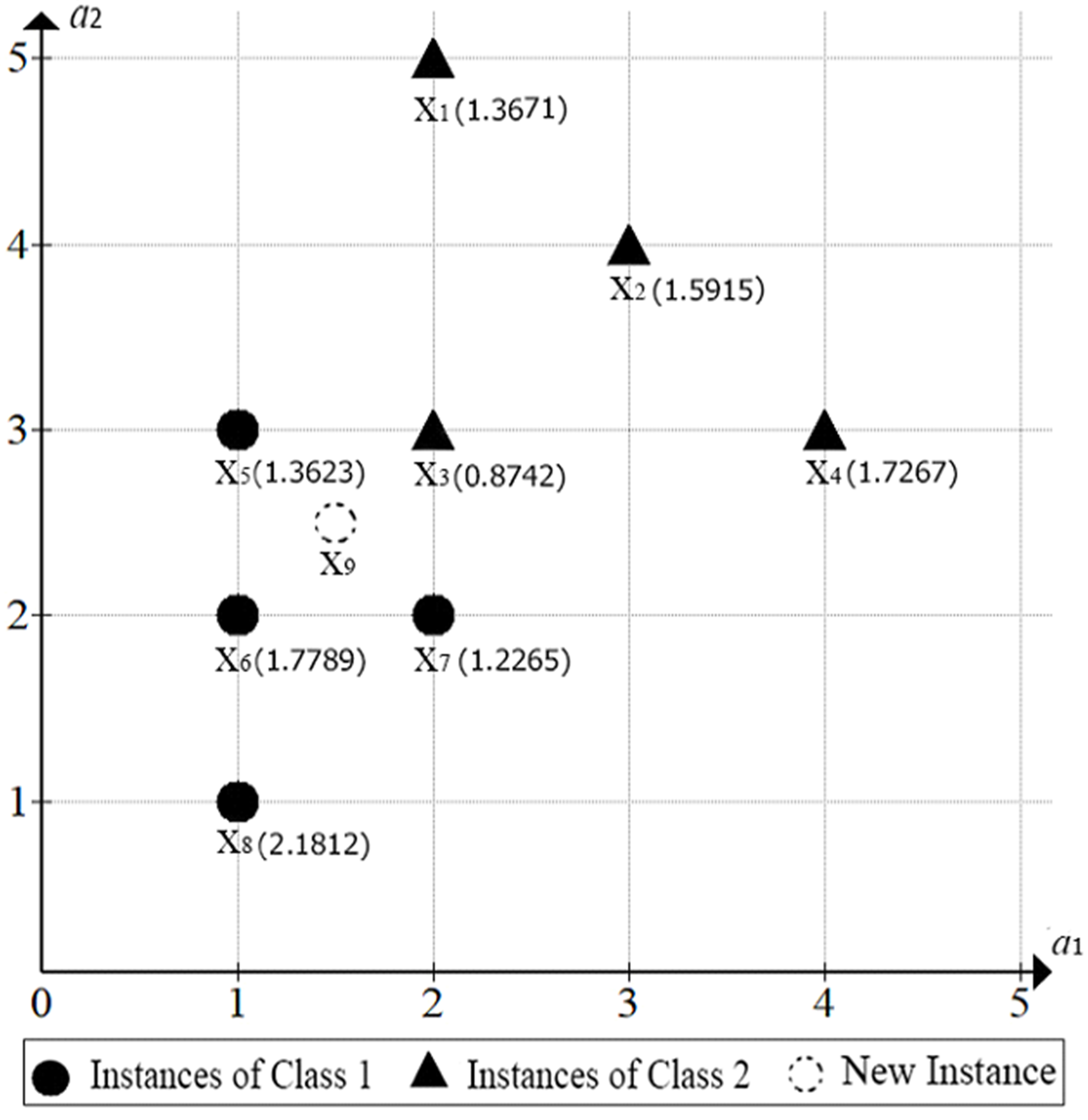 $x_{1}$ , $x_{2}$ , $x_{3}$ , $x_{4}$ , $x_{5}$ , $x_{6}$ , $x_{7}$ , $x_{8}$ } described in Table 3 and a new instance ( $x_{9}$ ), represented by the dashed circle in the figure, to be classified.

5. Methodology, experiments, results and analysis

#Id	$a_{1}$	$a_{2}$	Class
$x_{1}$	2	5	2
$x_{2}$	3	4	2
$x_{3}$	2	3	2
$x_{4}$	4	3	2
$x_{5}$	1	3	1
$x_{6}$	1	2	1
$x_{7}$	2	2	1
$x_{8}$	1	1	1

To investigate the performance of the NN tiebreaker criterion based on the value of instance typicality, first a group of 25 sets of instances was selected from the UCI Repository [13] with focus on promoting a diverse group of data sets, taking into account number of instances, number of attributes, types of attributes, presence or not of identical instances in the set, presence or not of contradictory instances in the set. Table 5 describes some of the characteristics of each data set.

Table 5
Description of the main characteristics of the 25 sets of instances used in the experiments, where columns: Dataset: name of the dataset, #I: number of instances, #Identical: number of identical instances, #Contradictory: number of contradictory instances, #CA: number of continuous attributes describing the instances and #NA: number of nominal attributes describing the instances

Dataset	#I	#Identical	#Contradictory	#CA	#NA
Australian	690	0	0	8	6
Balance	625	0	0	0	4
Banana	5,300	8	1	2	0
Breast	277	14	6	0	9
Bupa	345	4	0	6	0
Car	1,728	0	0	0	6
Chess	3,196	0	0	0	36
Coil2000	9,822	1,442	119	1	84
Contraceptive	1,473	48	67	2	7
Dermatology	358	0	0	0	35
Flare	1,066	701	78	0	11
Haberman	306	17	6	3	0
Hayes.roth	160	67	9	0	4
Housevotes	231	72	0	0	16
Iris	150	3	0	4	0
Led7Digit	500	354	61	0	7
Lymphography	148	0	0	0	18
Mammographic	830	266	45	1	4
Marketing	6,876	625	620	0	13
Monk.2	432	0	0	0	6
Mushroom	5,644	0	0	0	22
Optdigits	5,620	0	0	0	64
Tae	151	41	4	0	5
Titactoe	958	0	0	0	9
Zoo	101	42	0	0	16

For the choice of the sets of instances used in the experiments, the criterion of testing different structures was used. In order to implement the criterion, the average of the typicality values of the instances, in each data set, was calculated, considering that the average value of typicality indicates whether the set has an embedded gradual structure i.e., there is a great variation in the values of the instances in the set. The sets used in the experiments have their corresponding typicality average values ranging from 0.9304 to 2.4813 where the average of their typicality values is 1.3537.

Other factors that directly influence the instance’s typicality, such as the number of instances and the number of attributes that describe the instances, were also taken into account when choosing the data sets. As for the number of instances, sets having between 101 and 9,822 instances were used, with an average of 1,730 instances per set. As for the number of attributes describing instances, the sets have numbers between 2 and 85, with an average of 16 attributes describing the instances.

Table 6

Accuracy values, where columns are named as follows. Data set: name of the data set, Average Typicality: average of the typicality of the instances in Data set, NN Accuracy(%): using as tiebreaker criteria the random choice of nearest neighbor instance, NNtip-Accuracy(%): using as tiebreaker criteria the instance with the lowest value of typicality and NNtip+Accuracy(%): using as tiebreaker criteria the instance with the highest value of typicality

Data set	Average typicality	NN accuracy(%)	NNtip- accuracy(%)	NNtip+ accuracy(%)
Australian	1.1350	82.1739	82.1739	82.1739
Balance	1.4877	56.9925	44.6568	87.9948
Banana	1.0093	87.5849	87.5660	87.6038
Breast	1.1688	72.1534	82.5168	75.4565
Bupa	1.0011	64.1020	64.3876	63.8162
Car	1.3218	75.4655	70.0235	63.0189
Chess	1.0366	85.2152	84.3681	87.1318
Coil2000	1.0111	89.5235	89.4523	89.3607
Contraceptive	1.0281	44.0646	44.1336	44.2692
Dermatology	1.4990	94.6742	92.7289	96.6345
Flare	1.2851	69.6077	58.3504	72.1434
Haberman	0.9304	65.0323	64.3763	66.0000
Hayes.roth	1.4181	70.6250	78.1250	68.7500
Housevotes	2.4813	91.4789	91.6144	90.8753
Iris	1.4831	96.0000	96.0000	96.0000
Led7Digit	1.8776	63.6000	29.0000	72.6000
Lymphography	1.2835	87.4118	83.5518	87.4118
Mammographic	1.6457	73.7727	70.1262	79.1317
Marketing	1.1886	28.2027	23.0951	29.8298
Monk.2	1.2879	90.9147	49.6957	81.7030
Mushroom	1.4769	100.000	100.000	100.0000
Optdigits	1.2190	89.0392	89.9822	87.4677
Tae	1.2400	65.6250	60.3750	66.9167
Titactoe	1.0849	67.0885	64.8791	72.9866
Zoo	2.2422	95.8333	97.5000	96.666
Average	1.3537	76.2473	71.9471	77.8377

Considering the work had its focus on nominal attributes, 17 out of 25 have their corresponding instances described only by nominal attributes, 4 out of 25 have occurrences of both types of attributes i.e., nominal and continuous and 4 datasets have their corresponding instances described only by attributes of continuous type. The low number of data sets with continuous attributes only is due to the nature of the attribute values (real numbers) that describe their instances; the occurrence of a tie in an IBL environment where the stored instances are vectors of real numbers, is not a frequent event. However, if the number of attributes that describe the instances is quite small, eventually a tie may occur, particularly when the real values in question are integers values.

In a ML learning environment the choice of data sets for running experiments, whether having real-world or artificial data, usually has the purpose of evaluating the performance and computational cost of ML algorithms, under certain conditions. Particularly such choice, in the context of the work reported in this article, aimed at evaluating the influence of the data structures embedded in the data, as well as the presence of identical instances and contradictory instances impacts the proposed strategy In this work attributes of binary type were treated as nominal attributes. However, it is important to note that for the NN algorithm, using the HOEM distance function, attributes having binary values can be treated as continuous, without any change in the final result, as long as the binary values are numerically represented by values 0 and 1.

Each data set was used in a 10-cross-validation process [27] taking into account three different strategies of breaking ties. As discussed earlier in this work, a tie happens when the distance function used by the NN algorithm during the classification phase of the algorithm identifies more than one instance as the nearest neighbor of the instance to be classified. The three tiebreaker strategies considered are (1) the class of the new instance is randomly chosen among the classes of its nearest neighbors, (2) the new instance is classified with the class of its nearest instance with the smaller value of typicality (identified as NNtip-); (3) the new instance is classified with the class of its nearest instance with the highest value of typicality (identified as NNtip+). Results from the 25 experiments involving the execution of 10-cross-validation processes can be seen in Table 6.

As well-known throughout ML literature, the cross validation process is a validation strategy for assessing the predictive performance of the concept induced by a ML algorithm, based on a training data, on new data (testing data). Usually the strategy is referred to as k-fold cross validation, where parameter k represents the number of parts the original data should be divided into, as well as the number of times the process is repeated, usually using ( $k-1$ ) parts as training data and the remaining one as testing data. It is important to mention that, due to the adoption of a k-fold cross validation process, an instance may present typicality values slightly different among the $k-1$ training sets it is part of.

As it can be confirmed in the numbers shown in Table 6, the NNtip+ obtained the highest average value among the 25 datasets, taking into account the three strategies employed i.e., 77.8377%, against the average accuracy of 76.2473% reached by the random strategy and the average accuracy of 71.7602% reached by the NNtip-. The difference in results between choosing the nearest neighbor with the lowest typicality and the nearest neighbor with the highest typicality reinforces the influence of typicality as a good criteria to be considered for tiebreaker.

Analyzing the results taking into account the instance sets individually, it can be seen that the NNtip+ had the best results in 12 out of the 25 data sets and in 5 of them, the accuracy results were 5% higher. In 3 out of the 25 data sets, the results obtained by the NN implementing the random tiebreaker results had the best accuracy values. The NNtip- obtained the best accuracy results in 6 data sets; in 2 of them, particularly, had expressively better results. It is important to mention that in 3 data sets there was no occurrence of ties and, as a consequence, the use of the NN with each of the three strategies had results with the same accuracy.

Among the data sets that have not presented any tie situation, three different data configurations were observed: (1) the Iris data set, with 150 data instances described by 4 continuous attributes, (2) the data set Australian, with 690 data instances, described by 8 continuous attributes and 6 nominal attributes and (3) the mushroom data set that, despite having only attributes of the nominal type (whose number is 22), correctly classifies all instances tested in the three situations.

In the conducted experiments based on the Lymphograph data set, the results given by the NN and the NNtip+ had the same accuracy, which could be considered a coincidence provoked by the NN’s random tiebreaker.

The low average typicality of instances, in data sets where instances are described by continuous attributes namely, the Banana data set, with average typicality of 1.0093, the Bupa data set, with average typicality of 1.0011 and the Haberman data set, with average typicality of 0.9304, are evidence that the concept of typicality is not suitable to be used for implementing measures related to data sets whose instances are described by attributes of continuous type.

In relation to results related to the values of the average typicality, in sets whose instances are described by continuous attributes, the data set Iris stands out, considering its average typicality value is 1.4831. However, as there were no ties in this set, the classification accuracy results were the same for the three situations considered. As can be seen in Fig. 4, the set Iris has a high intra-conceptual similarity and a low inter-conceptual similarity; however, the continuous values that describe the four attributes are enough to distinguish each instance so that there are no ties.

Figure 4.

Relationships between the four attributes that describe instances of the Iris data set.

As far as the results of the experiments are concerned, the most expressive differences among the results related to precision occurred when the corresponding data set was of medium size, and its instances described by a few attributes e.g, between 4 and 9 attributes. However, among the sets with such characteristics, there are those that have identical instances as well as contradictory instances, as in the Hayes.roth, Led7digit and Mammographic data sets, as well as those that do not have these types of instances, as is the case of the Balance and the Tictactoe data sets, showing that tie situations are not only exclusive to data sets that have contradictory instances.

6. Final remarks

This paper reports the proposal of a strategy to be used during the classification phase of instance-based learning algorithms and particularly, of the well-known Nearest Neighbor (NN) algorithm. The strategy is based on the concept of typicality of an instance, used as a tiebreaker in situations where the instance to be classified has more than one nearest neighbor. The motivation for the proposal of the strategy was the fact that the strategy adopted by the original NN, in situations of ties, is the random choice between the nearest neighbors of the new instance to be classified. As pointed out in sections of this paper, the concept of typicality is particularly relevant when instances are also described by attributes having nominal type.

It can be found in the literature several other proposals of distance functions for nominal attributes that can be considered more refined alternatives than the simplistic value overlap used by the HEOM. Among them, the Value Difference Metric (VDM) [33], that defines the distance between two values $x_{a}$ and $y_{a}$ of an attribute a to reflect the fact that the two values are closer if they are used for describing instances of the same class. However, empirical results indicate that the HEOM distance function has classification accuracy higher than the original Euclidean distance function and, also, preserves approximately the same computational efficiency [38].

The results of the conducted experiments, presented in Section 5, are evidence that the use of the typicality values of the instances involved in a tie situation, tend to help a better choice of the more representative instance of the concept, among them. The help typicality provides can particularly favor data described by nominal attributes. The work described in this paper will be continued by considering other tiebreaker criteria, involving also the use of the information contained in the performance classification records associated with each stored instances, as implemented by algorithms of the IBL family [3]. Instance-based learning algorithms as well as any other ML algorithm can benefit from pre-processing the set of instances aiming at the removal of contradictory instances.

Footnotes

Acknowledgments

Authors are grateful to UNIFACCAMP, Campo Limpo Paulista, S. Paulo, Brazil, for the support received throughout the period this work was developed. The second author is also thankful to the Conselho Nacional de Desenvolvimento Científico e Tecnológico (CNPq). This study was financed in part by the Coordenação de Aperfeiçoamento de Pessoal de Nível Superior – Brazil (CAPES) – Finance Code 001.

References

Aha

D.W.

Kibler

and Albert

M.K.

, Instance-based learning algorithms, Machine Learning 6 (1991), 37–66.

Aha

D.W.

, Tolerating noisy, irrelevant and novel attributes in instance-based learning algorithms, International Journal of Man-Machine Studies 36 (1992), 267–287.

Aha

D.W.

, Ed., Lazy Learning, Springer Science+Business Media Dordrecht, 2013.

Ahmad

and Dey

, K-mean clustering algorithm for mixed numeric and categorical data, Data & Knowledge Engineering 63 (2007), 503–527.

Alcalá-Fdez

Fernandez

Luengo

Derrac

García

Sánchez

and Herrera

, KEEL Data-mining software tool: data set repository, integration of algorithms and experimental analysis framework, Journal of Multiple-Valued Logic and Soft Computing 17 (2011), 255–287, https://sci2sugr.es/keel/datasets.php.

Barsalou

, Ideals, central tendency, and frequency of instantiation as determinants of graded structure in categories, Journal of Experimental Psychology: Learning, Memory and Cognition 11 (1985), 629–624.

Berthold

M.R.

Borgelt

Höppner

and Klawonn

, Guide to Intelligent Data Analysis, Springer-Verlag London Limited, 2010.

Bishop

C.M.

, Pattern Recognition and Machine Learning, Springer-Verlag New York Inc, 2011.

Breiman

Friedman

Stone

C.J.

and Olshen

R.A.

, Classification and Regression Trees, CRC Press, 1984.

10.

Brighton

and Mellish

, Advances in instance selection for instance-based learning algorithms, Data Mining Knowledge Discovery 6 (2002), 153–172.

11.

Cost

and Salzberg

, A weighted nearest neighbor algorithm for learning with symbolic features, Machine Learning 10 (1993), 57–78.

12.

Cover

and Hart

, Nearest neighbor pattern classification, IEEE Transactions on Information Theory 13 (1967), 21–27.

13.

Dua

and Graff

, UCI Machine Learning Repository [http://archive.ics.edu/ml]. Irvine, CA: University of California, School of Information and Computer Science, 2019.

14.

Duda

R.O.

Hart

P.F.

and Stork

D.G.

, Pattern Classification, USA: John Wiley & Sons, Inc, 2001.

15.

Gan

and Wu

, Data Clustering Theory, Algorithms, and Applications, ASA/SIAM Publishers, 2007.

16.

Gates

G.W.

, The reduced nearest neighbor rule, IEEE Transactions on Information Theory 18(3) (1972), 431–433.

17.

Giraud-Carrier

and Martinez

, An efficient metric for heterogeneous inductive learning applications in the attribute-value language, Intelligent Systems (1995), 341–350.

18.

Gonçalves

S.V.

and Nicoletti

M.C.

, A proposal based on instance typicality for dealing with nominal attribute values in instance-based learning environments, In: Proc. of the 19th International Conference on Intelligent Systems Design and Application (ISDA 2019) (scheduled to be published in April-May 2020), 2019.

19.

Grochowski

and Jankowski

, Comparison of instance selection algorithms II, results and comments, Lecture Notes in Computer Science, Springer Verlag, v. 3070, 2004, pp. 580–585.

20.

Han

Kamber

and Pei

, Data Mining – Concepts and Techniques, Amsterdam: Morgan Kaufmann Publishers, 2012.

21.

Hart

P.E.

, The condensed nearest neighbor rule, IEEE Transactions on Information Theory 14 (1968), 515–516.

22.

L.-Y.

Huang

M.-W.

S.-W.

and Tsai

C.-F.

, The distance function effect on k-nearest neighbor classification for medical datasets, SpringerPlus 5(1304) (2016). doi: 10.1186/s40064-016-2941-7.

23.

Kadir

Nugroho

L.E.

Susanto

and Insap

P.S.

, Experiments of distance measurements in a foliage plant retrieval system, International Journal of Signal Processing, Image Processing and Pattern Recognition 5(2) (2012), 47–60.

24.

Kataria

and Singh

M.D.

, A review of data classification using K-nearest neighbour algorithm, International Journal of Emerging Technology and Advanced Engineering 3(6) (2013), 354–360.

25.

Manning

C.D.

Raghavan

and Schutze

, An Introduction to Information Retrieval, Cambridge University Press, Cambridge, 2008.

26.

Mitchell

T.M.

, Machine Learning, McGraw-Hill, New York, 1997.

27.

Moreno-Torres

J.G.

Sáez

J.A.

and Herrera

, Study on the impact of partition-induced dataset shift on k-fold cross-validation, IEEE Transactions on Neural Networks and Learning Systems 23 (2012), 1304–1312.

28.

Muggleton

S.H.

, Inductive logic programming, New Generation Computing 8(4) (1991), 295–318.

29.

Muggleton

S.-H.

, Inductive logic programming: issues, results and the challenge of learning language in logic, Artificial Intelligence 114(1–2) (1999), 283–296.

30.

Ritter

G.L.

Woodruff

H.B.

Lowry

S.R.

and Isenhour

T.L.

, An algorithm for the selective nearest neighbour decision rule, IEEE Transactions on Information Theory 21(6) (1975), 665–669.

31.

Rosch

and Mervis

C.B.

, Family resemblances: studies in the internal structure of categories, Cognitive Psychology 7(4) (1975), 573–605.

32.

Schul

and Burnstein

, Judging the typicality of an instance: should the category be accessed first? Journal of Personality and Social Psychology 58(6) (1990), 964–974.

33.

Stanfill

and Waltz

, Toward memory-based reasoning, Communications of the ACM 29(12) (1986), 1213–1228.

34.

Todeschini

Consonni

Grisoni

F.G.

and Ballabio

, A new concept of higher-order similarity and the role of distance/similarity measures in local classification methods, Chemometrics and Intelligent Laboratory Systems 157 (2016), 50–57.

35.

Wilson

D.L.

, Asymptotic properties of nearest neighbor rules using edited data, IEEE Transactions on Systems, Man, and Cybernetics SMC-2 (1972), 408–421.

36.

Willett

Barnard

J.M.

and Downs

G.M.

, Chemical similarity searching, Journal of Chemical Information and Computer Sciences 38(6) (1998), 983–996.

37.

Wilson

D.R.

and Martinez

T.R.

, Reduction techniques for instance-based learning algorithms, Machine Learning 38 (2000), 257–286.

38.

Wilson

D.R.

and Martinez

T.R.

, Improved heterogeneous distance function, Journal of Artificial Intelligence Research 6 (1997), 1–34.

39.

Kumar

Quinlan

J.R.

Ghosh

Yang

Motoda

McLachlan

G.J.

Liu

P.S.

Zhou

Z.-H.

Steinbach

Hand

D.J.

and Steinberg

, Top 10 algorithms in data mining, Knowledge and Information Systems 14(1) (2008), 1–37.

40.

Zhang

, Selecting typical instances in instance-based learning, In: Proceedings of the Ninth International Machine Learning Conference, 1972, pp. 470–479.

Using the concept of instance typicality in instance-based learning environments involving nominal attributes

Abstract

Keywords

1. Introduction

2. Earlier instance-based learning algorithms

Table 1 Identification of the six attributes and the class that describe each instance of the Car dataset. The table also shows the possible values associated to the six attributes and to the class (Acceptability)

Footnotes

Acknowledgments

References

Table 1
Identification of the six attributes and the class that describe each instance of the Car dataset. The table also shows the possible values associated to the six attributes and to the class (Acceptability)