Comparing different metrics on an anisotropic depth completion model

Abstract

This paper discussed an anisotropic interpolation model that filling in-depth data in a largely empty region of a depth map. We consider an image with an anisotropic metric $g_{ij}$ that incorporates spatial and photometric data. We propose a numerical implementation of our model based on the “eikonal” operator, which compute the solution of a degenerated partial differential equation (the biased Infinity Laplacian or biased Absolutely Minimizing Lipschitz Extension). This equation’s solution creates exponential cones based on the available data, extending the available depth data and completing the depth map image. Because of this, this operator is better suited to interpolate smooth surfaces. To perform this task, we assume we have at our disposal a reference color image and a depth map. We carried out an experimental comparison of the AMLE and bAMLE using various metrics with square root, absolute value, and quadratic terms. In these experiments, considered color spaces were sRGB, XYZ, CIE- $L^{*}a^{*}b^{*}$ , and CMY. In this document, we also presented a proposal to extend the AMLE and bAMLE to the time domain. Finally, in the parameter estimation of the model, we compared EHO and PSO. The combination of sRGB and square root metric produces the best results, demonstrating that our bAMLE model outperforms the AMLE model and other contemporary models in the KITTI depth completion suite dataset. This type of model, such as AMLE and bAMLE, is simple to implement and represents a low-cost implementation option for similar applications.

Keywords

Biased absolutely minimizing lipschitz extension bilateral filter depth completion

1. Introduction

Depth maps are widely used in autonomous vehicles, autonomous aircraft, 3D modeling for BIM (Building Information Modelling) systems, and game consoles such as the Xbox. Depth maps frequently present a lack of acquired data or data with low confidence levels. Occlusions and sensor misinterpretation of acquired data (ToF camera, LiDAR, or a Kinect sensor) result in holes in the acquired depth map.

This paper discusses anisotropic depth data completion applied to the interpolation of depth maps in large empty regions. Our proposal aims to fill the empty data region of a depth image with two elements: i) data from the self depth image and ii) a corresponding color image known as the reference image. This paper presents an empirical analysis of a depth map completion interpolation operator. The biased Absolute Minimizing Lipschitz Extension, also known as the biased Infinity Laplacian or bAMLE, is an interpolation operator that first appeared in the axiomatic approach proposed in [1, 2].

The AMLE interpolator was introduced in [3, 4] as a completion method from a theoretical point of view. As explained in [2, 1], the infinity Laplacian operator is simple and satisfies a small set of mathematical axioms. This work proposed a computational scheme to solve the biased Infinity Laplacian using the “eikonal” operator to obtain a numerical implementation. This numerical implementation produces a weighted average-based numerical model of the biased Infinity Laplacian, which is fast and straightforward to implement.

1.1 Related works

The goal of the depth completion task is to estimate or recover dense depth maps from sparse data. Some depth completion methods rely solely on the depth data available, while others rely on additional data such as a scene color reference image. The goal of methods that use a color reference image or (guided methods) is to perform depth completion using a color image while avoiding creating new objects that are not present in the original image [5]. Image enhancement [6], depth inpainting [7], filtering, and various other tasks that have all benefited from guided methods. The main idea behind guided filters is that meaningful information from the color reference image, such as textures and edges, can be transferred to the incomplete depth map.

A bilateral filter is an image domain-spatial filter that focuses on local features like edges or smoothness of the image to guide the filtering. This filter is frequently used to filter and input image [7] preserving strong edges [8].

In [9] is proposed a method that simultaneously recovers a depth map and reconstructs a gray level image of the scene. To perform this task, the authors use convolutional neural networks (CNN). This scheme outperforms methods that used only depth in the KITTI depth completion suite benchmark [10]. In [11] is proposed a model to solve the problem of depth completion outside the object in the scene. The authors use CNN and a new representation for depth called Depth Coefficients (DC). This representation lets them avoid inter-object depth mixing. The authors of [5, 12] evaluated convolutional networks in a database containing depth images captured by a Kinect sensor. The authors used CNN to complete the data after down-sampling these depth images every other 8 pixels square.

In [13] an approach to classify disturbed depth data by learning an input trust estimator based on normalized convolutional neural networks is presented (NCNNs).

Application to depth completion of AMLE filter was performed in either elevation models [14] or optical flow completion [15].

The bAMLE was applied to complete depth data in [16], but the authors did not test different metrics or color spaces.

Recently in [17] the interpolations properties of the AMLE operator have been applied to the flow densification and large hole completion in optical flow. The work in [18] presents a method that simultaneously semantically segment the scene and depth completion under a multi-task deep learning framework. The authors proposed a scheme that considers one encoder used semantically to segment the scene and also for depth completion. The authors introduced boundary features used in the decoder. An extra boundary module was used to generate boundary features constructing a cross-task joint loss function for the training stage. Experimentally, the authors demonstrated that the proposal can jointly improve both estimations. In [19] is proposed a method to complete depth maps. To complete depth the authors use a binary anisotropic diffusion tensor. The authors also proposed an image-guided nearest neighbor search used by the binary tensor. This paper proposed a variational scheme that consists of a data term and a regularization term. The proposal due to its anisotropy preserves discontinuities in the image of the scene between different objects, i.e. generate piece-wise constant depth maps. Results show that the methods perform well in recovering flat surfaces.

The work in [20] presents a deep learning approach to solve the problem of depth completion. The authors use a depthwise separable technique to reduce the number of parameters of the net. They use that technique in the convolution and deconvolution stages. They reduced number of parameters in a 96% keeping the performance similar to the state of the art methods. Finally, they implemented their proposal in FPGA reaching processing time of 11 images per second.

This paper is an extended version of our original manuscript presented in [16].

The contribution of this extended manuscript are three folds:

iii) i)
Test the numerical implementation of the AMLE and bAMLE using new metrics, which use fractional exponent ( $\mathcal{L}^{\frac{1}{2}}$ , $\mathcal{L}^{1}$ , $\mathcal{L}^{2}$ ) and.
ii)
Test the implementation using different color spaces (sRGB, XYZ, $L^{}a^{}b^{*}$ and CMY).
iii)
The best parameter for the proposal were estimated using PSO (Particle Swarm Optimization) and EHO (Elephant Herd Optimization) and both performances were compared.
iv)
We filtered the final estimated depth with a median filter increasing the performance of the whole estimation.

In Section 2 we present the biased infinity Laplacian (bAMLE) we used to complete sparse disparities. In Section 2.2 we explain our numerical implementation of the bAMLE and in Section 4 is presented the performance of our proposal in KITTI [21]. Finally, Section 5 presents our conclusions.
2. Method

The bAMLE (biased infinity Laplacian) first appeared in the analysis of interpolators in manifolds [1, 2], but it was not evaluated there. In the context of sparse depth map completion, the bAMLE interpolator is very efficient in filling in blank areas in depth maps.

Dealing with the problem,

$\displaystyle\Delta_{\infty,g}u+\beta|\nabla u|_{\xi}=0\in\Omega,$ (1)

as well as the constraint $u|_{\partial\Omega}=\theta$ , $\Omega\subset\mathbb{R}^{2}$ is the problem domain, $g_{ij}$ is the metric and, $\xi$ is the direction of the gradient, $\beta\in\mathbb{R}^{+}$ , $\nabla u$ gradient of the depth map, $\Delta_{\infty,g}u$ depth map infinity Laplacian given the metric $g_{ij}$ and $\Delta_{\infty,g}u:=D^{2}_{\mathcal{M}}u\left(\frac{\nabla u}{{|\nabla u|}_{% \xi}},\frac{\nabla u}{{|\nabla u|}_{\xi}}\right)$ with $\mathcal{M}$ $=(\Omega,g)$ the manifold. The metric $g_{ij}$ measures the geodesic spatial and photometric similarity between pixels of a reference image. We considered the term:

$\displaystyle D^{2}_{{\mathcal{M}},ij}u(\mathbf{x})=\frac{\partial^{2}u}{% \partial x^{i}\partial x^{j}}(\mathbf{x})-\Gamma_{ij}^{k}(\mathbf{x})\frac{% \partial u}{\partial x^{k}}(\mathbf{x}),$

where $\Gamma^{k}_{ij}$ is the Christoffel symbol in the coordinates system and the indices $i$ . $j$ , $k=1,2$ . When $\beta=0$ Eq. (1) became the AMLE equation. We consider Eq. (1) in the viscosity sense. Given this notation we write again Eq. (1):

$\displaystyle\frac{1}{|\nabla u(\mathbf{x})|_{x}^{2}}D^{2}_{{\mathcal{M}},ij}u% (\mathbf{x})g^{i\alpha}(\mathbf{x})\frac{\partial u}{\partial x^{\alpha}}(% \mathbf{x})g^{j\gamma}(\mathbf{x})\frac{\partial u}{\partial x^{\gamma}}(% \mathbf{x})$ $\displaystyle+\beta|\nabla u(\mathbf{x})|_{x}=0,$ (2)

where

$\displaystyle|\nabla u(\mathbf{x})|_{x}^{2}=g^{ij}(\mathbf{x})\frac{\partial u% }{\partial x^{i}}(\mathbf{x})\frac{\partial u}{\partial x^{j}}(\mathbf{x}).$

2.1 AMLE and biased-AMLE

Let $I:\Omega\subset\mathbb{R}^{2}\rightarrow\mathbb{R}^{3}$ a color reference image and $u(\mathbf{x}):\Omega\rightarrow\mathbb{R}$ is the scene depth data. Supposing that the available data is located in a region $O\subset\Omega$ with a boundary $\partial O$ . We endowed the domain $\Omega$ with a metric $g$ with these two elements we have constructed a Riemannian manifold $(\Omega,g)$ .

Let us describe a particular case which is of interest for us here. Assuming that $g_{ij}(\mathbf{x})=h(\mathbf{x})\delta_{ij}$ i.e. $h(\mathbf{x})=(\kappa_{1}+\kappa_{2}|\nabla I(\mathbf{x})|^{2})^{p}$ . For some $p>0$ , where $I$ is a given image. Thus, we can write Eq. (2):

$\displaystyle\frac{1}{|\nabla u(\mathbf{x})|^{2}}D^{2}_{{\mathcal{M}},ij}u(% \mathbf{x})\frac{\partial u}{\partial x^{i}}(\mathbf{x})\frac{\partial u}{% \partial x^{j}}(\mathbf{x})$ $\displaystyle+\beta|\nabla u(\mathbf{x})|_{x}=0.$ (3)

In this case, $h(\mathbf{x})$ was canceled in the numerator and the denominator in the first term of the Eq. (2.1). It remains in the Christoffel symbols and the absolute value of the gradient in the second term. The task of interpolating sparse disparity maps is performed using a reference image and the incomplete disparity map. The Eq. (1) is discretized and solved according to [22, 23]. We suppose we have at our disposal a reference color image from which a geodesic distance between points can be computed. This biased AMLE will interpolate depth data on isolated points and perfectly will fit the available data. Because of this behavior, the interpolator may expand known data to wide empty areas. We can write also Eq. (2) as

$\displaystyle D^{2}_{{\mathcal{M}},ij}u(\mathbf{x})g^{i\alpha}(\mathbf{x})% \frac{\partial u}{\partial x^{\alpha}}(\mathbf{x})g^{j\gamma}(\mathbf{x})\frac% {\partial u}{\partial x^{\gamma}}(\mathbf{x})$ $\displaystyle+\beta|\nabla u(\mathbf{x})|_{x}^{3}=0$ (4)

The AMLE is usually obtained as the limit of $p\to\infty$ of minimizers of the energy,

$\displaystyle\int_{\Omega}|\nabla u|_{g}^{p}|g|^{1/2}{\rm d}x$ (5)

where $|g|=\det(g(x))$ satisfying specified Dirichlet boundary conditions. The case $p=2$ corresponds to the Dirichlet integral.

2.2 A numerical implementation for the biased Infinity Laplacian

Considering the discrete grid as a graph, let us take a pair of grid points $\mathbf{x},\mathbf{y}$ and let $d_{\mathbf{x}\mathbf{y}}$ be their distance. If the considered $\mathbf{x},\mathbf{y}$ are grid neighbors, $d_{\mathbf{x}\mathbf{y}}$ is computed by:

$\displaystyle d_{\mathbf{x}\mathbf{y}}=\sum_{i=1}^{3}\kappa_{c}|I_{i}(\mathbf{% x})-I_{i}(\mathbf{y})|^{p}+\kappa_{x}\|\mathbf{x}-\mathbf{y}\|^{p},$ (6)

where $\kappa_{c}$ , $\kappa_{x}$ , are constants $\in\mathbb{R}$ , $I(\mathbf{x})$ is the reference image with three color components given by the used color space and $p\in\mathbb{Q}$ .

Let us take a curve $\{\gamma(i)\}_{i=0}^{m}$ in the grid, its length $L_{g}(\gamma)$ is given by:

$\displaystyle L_{g}(\gamma)=\sum_{i=0}^{m}d_{\gamma(i),\gamma(i+1)}.$ (7)

Given a pair of points $\mathbf{x}$ and $\mathbf{y}$ in the grid, the distance $d$ could be defined by:

$\displaystyle d=$ (8) $\displaystyle\inf\{L_{g}(\gamma):\hbox{\rm$\gamma$ is a curve from $\mathbf{x}% $ joining to $\mathbf{y}$}\}.$

The distance $d$ should be computed using Dijkstra’s algorithm.

The discretization model proposed in [16] is fundamental for the proposal we recalled here. Given a point $\mathbf{x}$ in the grid, let $\mathcal{N}(\mathbf{x})$ be a neighborhood around $\mathbf{x}$ .

Based on the “eikonal” operator, the AMLE following [23] is given by:

$\displaystyle\Delta_{\infty,g}u(\mathbf{x})=$ (9) $\displaystyle{\displaystyle\frac{\max\limits_{\mathbf{y\in\mathcal{N}(x)}}{% \displaystyle\frac{u(\mathbf{y})-u(\mathbf{x})}{d_{\mathbf{x}\mathbf{y}}}}+% \min\limits_{\mathbf{z}\in\mathcal{N}(\mathbf{x})}{\displaystyle\frac{u(% \mathbf{z})-u(\mathbf{x})}{d_{\mathbf{x}\mathbf{z}}}}}{2}}$

The discretized version of the biased Infinity Laplacian corresponds to:

$\displaystyle\frac{\max\limits_{\mathbf{y\in\mathcal{N}(x)}}{\displaystyle% \frac{u(\mathbf{y})-u(\mathbf{x})}{d_{\mathbf{x}\mathbf{y}}}}+\min\limits_{% \mathbf{z}\in\mathcal{N}(\mathbf{x})}{\displaystyle\frac{u(\mathbf{z})-u(% \mathbf{x})}{d_{\mathbf{x}\mathbf{z}}}}}{2}$ $\displaystyle+\beta\left|\max\limits_{\mathbf{y\in\mathcal{N}(x)}}\frac{u(% \mathbf{y})-u(\mathbf{x})}{d_{\mathbf{x}\mathbf{y}}}\right|=0,$ (10)

with $\beta>0$ the Eq. (2.2) depends on the sign of the positive eikonal operator, $\max_{\mathbf{y\in\mathcal{N}(x)}}\frac{u(\mathbf{y})-u(\mathbf{x})}{d_{% \mathbf{x}\mathbf{y}}}$ , we obtain:

$\displaystyle u(x)=\frac{\beta_{+}d_{\mathbf{x}\mathbf{z}}u(\mathbf{y})+\beta_% {-}d_{\mathbf{x}\mathbf{y}}u(\mathbf{z})}{\beta_{+}d_{\mathbf{x}\mathbf{z}}+% \beta_{-}d_{\mathbf{x}\mathbf{y}}}.$ (11)

The numerical implementation for the iterative discretized biased Infinity Laplacian is:

$\displaystyle u^{k+1}(\mathbf{x})=\frac{\beta_{+}d_{\mathbf{x}\mathbf{z}}u^{k}% (\mathbf{y})+\beta_{-}d_{\mathbf{x}\mathbf{y}}u^{k}(\mathbf{z})}{\beta_{+}d_{% \mathbf{x}\mathbf{z}}+\beta_{-}d_{\mathbf{x}\mathbf{y}}},$ $\displaystyle k=0,1,\ldots$ (12)

with $\beta_{+}=\frac{1}{2}+\beta\text{sgn}\left(\max_{\mathbf{y\in\mathcal{N}(x)}}% \frac{u(\mathbf{y})-u(\mathbf{x})}{d_{\mathbf{x}\mathbf{y}}}\right)$ and $\beta_{-}=\frac{1}{2}$ .

2.3 Distance approximation

In practice, we have used the distance $d_{\mathbf{xy}}$ defined in Eq. (6) to approximate the length of the geodesic path ( $L_{g}$ ) (joining two points $\mathbf{x}$ and $\mathbf{y}$ ). Different neighborhood sizes, such as the 4-connected pixels of $\mathbf{x}$ or the 8-connected pixels of $\mathbf{x}$ , can be used. We use the approximated value of the distance $L_{g}\approx d_{\mathbf{x}\mathbf{y}}$ when using a larger neighborhood size.

2.4 Temporal extension

We have extended the AMLE and the biased AMLE to handle temporal information. Let us consider two consecutive frames $u_{t-1}$ and $u_{t}$ of a depth video sequence. We suppose that the depth image $u_{t-1}$ has holes or missing data. We propose to take into account the available depth data in $u_{t-1}$ and the available depth data in the consecutive frame $u_{t}$ in the video sequence as well as the reference video. We suppose that there is an available optical flow computed from the color video sequence. We use this optical flow to compensate (or warp) the depth map $u_{t}$ . With this new information we construct a new interpolation mask taking the information in $u_{t}$ and in $u_{t-1}$ .

Figure 1.

Color images and depth map for a video sequence. In the color images, a red balloon moves from left to right. We show the optical flow as a black arrow in frame 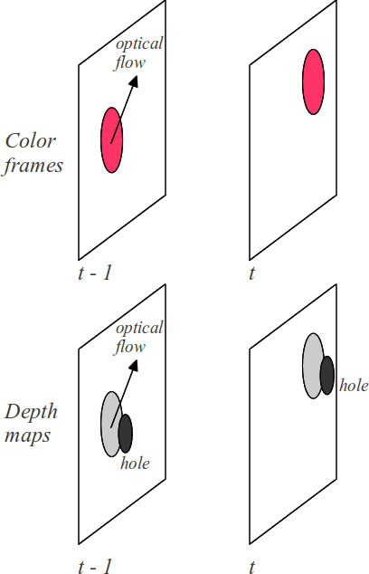$t-1$ . We show the depth map for the red balloon that moves and we show a hole in the depth map. The hole has the same motion as the object. No additional information can be obtained compensating the depth map by the optical flow.

We show in Fig. 1 a red balloon that moves from left to right. We also show the depth map of the balloon. There is a hole in the depth map that moves jointly with the balloon. By warping $u_{t}$ , we do not have new depth information. In Fig. 2, we show a slightly different situation. The red balloon moves from left to right, but the depth map hole does not move jointly with the object. When we compensate the depth data in $u_{t}$ , we have new depth information that helps to complete the depth data in $u_{t-1}$ .

Figure 2.

Color images and depth map for a video sequence. In the color images, a red balloon moves from left to right. The black arrow represents the optical flow. We show the depth map for the red balloon that moves and we show a hole in the depth map. In this example, the hole has a different motion of the object, which means that additional information can be obtained compensating the depth map by the optical flow.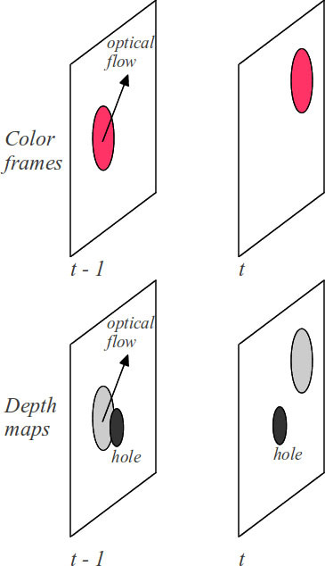

We have at our disposal a depth map $u_{t}$ of a depth video sequence and also a color reference image $I_{t}$ . The depth image can present a lack of information. If a lack of information is present (holes), we create a binary mask (if we have depth data, then mask $=$ 1, else mask $=$ 0). This mask represents the interpolation domain for our completion algorithm. The presented procedure described above is a tool to bring new information from the depth map in $u_{t}$ to the instant $t-1$ . With this new information, we modify the interpolation binary mask. With the new information, we fill holes of the binary mask, reducing the number of points to be interpolated, improving the quality of the interpolated depth map.

2.5 Color spaces

The metric presented in Eq. (6) considers a reference image in a specific color space. Our main idea is to evaluate the performance of the bAMLE model using many image color spaces. Three eye receptors give human color perception, which perceives a combination of three stimuli: Red, Green, and Blue. Different representation color models in digital images have been stated, taking into account aspects of human perception. We present transformations between the standard RGB (sRGB) model and other models.

2.5.1 sRGB to XYZ

In this space, $Y$ represents luminosity, $X$ is approximately blue color, and $Z$ represents approximately the red and green color. Defining $R^{\prime}$ , $G^{\prime}$ , and $B^{\prime}$ as:

$\displaystyle R^{\prime}=\frac{R}{255},$ $\displaystyle G^{\prime}=\frac{G}{255},$ $\displaystyle B^{\prime}=\frac{B}{255}.$ (13)

Computing variations in each component we have:

$\displaystyle\sigma_{R^{\prime}}=\begin{cases}100.0\left({\displaystyle\frac{R% ^{\prime}+0.055}{1.055}}\right)^{2.4}&R^{\prime}>0.04045\\ {\displaystyle\frac{100.0R^{\prime}}{12.92}}&R^{\prime}\leqslant 0.04045,\end{cases}$ (14) $\displaystyle\sigma_{G^{\prime}}=\begin{cases}100.0\left({\displaystyle\frac{G% ^{\prime}+0.055}{1.055}}\right)^{2.4}&G^{\prime}>0.04045\\ {\displaystyle\frac{100.0G^{\prime}}{12.92}}&G^{\prime}\leqslant 0.04045,\end{cases}$ (15)

and,

$\displaystyle\sigma_{B^{\prime}}=\begin{cases}100.0\left({\displaystyle\frac{B% ^{\prime}+0.055}{1.055}}\right)^{2.4}&B^{\prime}>0.04045\\ {\displaystyle\frac{100.0B^{\prime}}{12.92}}&B^{\prime}\leqslant 0.04045,\end{cases}$

then $X, Y, Z$ is given by:

$\displaystyle X=0.4124\sigma_{R^{\prime}}+0.3576\sigma_{G^{\prime}}+0.1805% \sigma_{B^{\prime}},$ $\displaystyle Y=0.2126\sigma_{R^{\prime}}+0.7152\sigma_{G^{\prime}}+0.0702% \sigma_{B^{\prime}},$ $\displaystyle Z=0.0193\sigma_{R^{\prime}}+0.1192\sigma_{G^{\prime}}+0.9595% \sigma_{B^{\prime}}.$ (17)

2.5.2 sRGB to CMY

This color space is composed by $C$ , $M$ and $Y$ . The conversion from sRGB to CMY is given by:

$\displaystyle C^{\prime}=1-R^{\prime},$ $\displaystyle M^{\prime}=1-G^{\prime},$ $\displaystyle Y^{\prime}=1-B^{\prime},$ $\displaystyle K^{\prime}=\min\{C^{\prime},M^{\prime},Y^{\prime}\},$ (18)

and the nonlinear transformation:

$\displaystyle C=\min\{1,\max\{0,C^{\prime}-Y^{\prime}\}\},$ $\displaystyle M=\min\{1,\max\{0,M^{\prime}-K^{\prime}\}\},$ $\displaystyle Y=\min\{1,\max\{0,Y^{\prime}-K^{\prime}\}\}.$ (19)

2.5.3 XYZ to CIE-L ${}^{*}a^{*}b^{*}$

Where $L^{*}$ represents perceptual lightning of the color, $a^{*}$ represents red and green color, and $b^{*}$ represents the blue and yellow color. Defining $\sigma_{x}$ , $\sigma_{y}$ , and $\sigma_{z}$ as:

$\displaystyle\sigma_{x}=\frac{X}{X_{r}},$ $\displaystyle\sigma_{y}=\frac{Y}{Y_{r}},$ $\displaystyle\sigma_{z}=\frac{Z}{Z_{r}},$ (20)

with $X_{r}=95.045$ , $Y_{r}=100.000$ and $Z_{r}=108.883$ are references at $D_{65}/2^{\circ}$ standard illuminant. Redefining $\sigma_{x}$ , $\sigma_{y}$ , and $\sigma_{z}$ as:

$\displaystyle\sigma_{x}=\begin{cases}\sqrt[3]{\sigma_{x}}&\sigma_{x}>0.008856% \\ 7.787\sigma_{x}+{\displaystyle\frac{16}{116}}&\sigma_{x}\leqslant 0.008856,% \end{cases}$ (21) $\displaystyle\sigma_{y}=\begin{cases}\sqrt[3]{\sigma_{y}}&\sigma_{y}>0.008856% \\ 7.787\sigma_{y}+{\displaystyle\frac{16}{116}}&\sigma_{y}\leqslant 0.008856\end% {cases}$ (22)

and,

$\displaystyle\sigma_{z}=\begin{cases}\sqrt[3]{\sigma_{z}}&\sigma_{z}>0.008856% \\ 7.787\sigma_{z}+{\displaystyle\frac{16}{116}}&\sigma_{z}\leqslant 0.008856.% \end{cases}$ (23)

Then $L^{*}$ , $a^{*}$ , and $b^{*}$ is given by:

$\displaystyle L^{*}=116\sigma_{y}-16,$ $\displaystyle a^{*}=500(\sigma_{x}-\sigma_{y}),$ $\displaystyle b^{*}=200(\sigma_{y}-\sigma_{z}).$ (24)

2.6 Algorithm to estimate parameters

We have estimated the parameters of AMLE (radius, $\kappa_{c}$ , $\kappa_{x}$ , and $n_{\text{iter}}$ ) using the PSO (Particle swarm optimization) algorithm [24]. This algorithm was used to estimate an optical flow model’s parameters described in [25]. The success of that previous work motivates us to use the PSO optimization algorithm in our proposal.

2.6.1 PSO algorithm

This algorithm optimizes a function by iteratively improving many candidate’ solutions. The algorithm performs each iteration updating those candidates. The updating of these candidates’ solutions is performed according to the dynamic positions and velocities of those candidates’ answers. In our case, those candidate solutions are different model parameters and the function to optimize is the depth estimation error. Let $f:\mathbb{R}^{n}:\rightarrow\mathbb{R}$ be the depth estimation error obtained by each candidate solution and $n$ is the number of the parameters to estimate. Let $\mu_{i}$ be a candidate solution that minimizes the depth estimation error with $i=1,\ldots,n$ . For each iteration, the best candidate solution is stored in $\mu_{b}$ , and also, the best candidate found in all performed iterations is stored in $\mu_{g}$ . The $\mu_{b}$ and $\mu_{g}$ are called the best candidate and best global candidate.

Each candidate solution ( $\mu_{i}$ ) are updated according to the evolution equation given by:

$\displaystyle\nu_{i}^{t+1}=\omega\nu_{i}^{t}+\varphi_{g}(\mu_{i}^{t}-\mu_{g})+% \varphi_{b}(\mu_{i}^{t}-\mu_{b})$ (25)

and,

$\displaystyle\mu_{i}^{t+1}=\mu_{i}^{t}+\nu_{i}^{t},$ (26)

where $\omega$ is the evolution parameter for each solution candidate $\mu_{i}$ , $\varphi_{g}$ and $\varphi_{b}$ are positive weight parameters, $\nu_{i}$ is the velocity for each candidate solution. A saturation for $\nu_{i}$ is usually incorporated. We used $\nu_{\max}=2$ and $\nu_{\min}=-2$ .

2.7 Elephant herd optimization (EHO)

Inspired by the behavior of an Elephant Herd, the EHO algorithm estimates the best solution to an optimization problem given a set of random solutions in an iterative scheme. An elephant in a clan represents each possible solution. Each Clan has a matriarch. In each iteration, a fixed number of elephants abandon the Clan. The matriarch is the individual that presents a better performance in the Clan. Let $x_{i}$ the individuals in each clan and $x_{i}[j]$ the $j$ -individual in the clan $i$ . Each individual in each Clan is updated according to:

$\displaystyle x_{i}[j]=x_{i}[j]+\alpha(x_{\text{best},i}-x_{i}[j])r,$

where $x_{\text{best},i}$ represents the matriarch in each clan, and $r$ is a random value in $[0,1]$ , $\alpha$ parameters represent the matriarch’s influence in her clan. Each

$\displaystyle x_{\text{best},i}=\beta x_{\text{center},i},$ (27)

and the center $x_{\text{center},i}$ was computed as the average of the individuals of the clan:

$\displaystyle x_{\text{center},i}=\frac{1}{n_{i}}\sum_{j=1}^{n_{i}}x_{i}[j],$ (28)

where $n_{i}$ is the number of individuals in each clan, and $i$ is the number of clans.

2.8 Implementation

We have implemented the algorithm in a GPU. Our implementation is not optimized, but it runs fast, reaching 0.096 seconds per iteration in images of 1216 $\times$ 352 pixels. The implementation was performed in a Notebook, Intel i7, 16 GB RAM, six cores, and GPU GTX1050 Ti. The CUDA version is nvcc 10.1.243, and the C compiler is gcc7.5.0 and running in Ubuntu 18.04.5.

Figure 3.

Example of RGB reference and depth images of the KITTI dataset. (a) (b) Example of color reference images of KITTI dataset. (c) and (d) Corresponding depth images of color reference images (a) and (b), respectively. Depth was color-coded using jet colormap in MATLAB.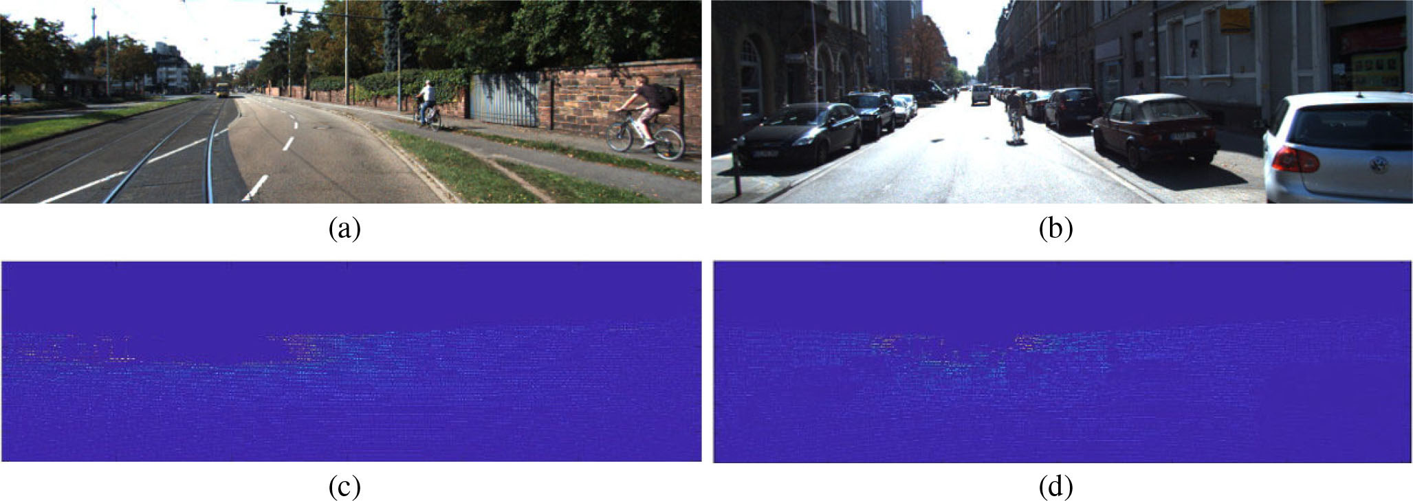

2.9 Pseudocode

In this section, we present the pseudocode of our algorithm to complete depth maps using bAMLE. We take the parameter value, the metric, the color space, and an occlusion mask indicating the interpolation region.

KwParParameters

[h] Depth completion using bAMLEOne color image $I$ of $N\times M$ pixels in a color space, interpolation mask $m$

$p,\text{radius},\kappa_{x},\kappa_{c},n_{\text{iter}},\beta^{-}$

Completed depth out

Initialization $\textit{out}=0$ .

$i\leftarrow 1$ to $n_{\text{iter}}$

$\mathbf{x}\leftarrow 1$ to $N\times M$

$m(\mathbf{x})==1$ Compute metric $d_{xy}$ for every pixel in the neighborhood $\mathcal{N}(\mathbf{x})$

Determine $u(\mathbf{y})$ that maximizes the positive eikonal operator in $\mathcal{N}(\mathbf{x})$ .

Determine $u(\mathbf{z})$ that minimizes the negative eikonal operator in $\mathcal{N}(\mathbf{x})$ .

Compute $\beta^{+}$ .

Update $u_{j}(\mathbf{x})$ according Eq. (2.2).

$\textit{out}=u_{i}$

$\mathbf{out}$ .

3. Data set and experiments

The KITTI depth completion suite includes 1000 RGB reference images as well as the corresponding depth ground truth. This ground truth is a semi-dense depth obtained from raw LiDAR scans.

In Fig. 3a and b we show two reference images. Figure 3c and d sparse depth images of the corresponding reference image.

MPI-Sintel is a synthetic data set publicly available constructed to evaluate optical flow estimation algorithms. The data set consists of a training set and a validation set. The training set is also divided into two subsets Clean and Final. The data set contains sequences of synthetic images where different effects are present: occlusions, small and fast displacements, blur, illumination changes, fog, the rapid motion of the camera, and many others. Figure 4 shows examples of consecutive images of the MPI-Sintel Final set.

Figure 4.

Examples of MPI-Sintel with color-coded ground truth. (a) and (b) frames 6 and 7 of sequences ambush_4, respectively. (c) color-coded optical flow. (d) and (e) frames 18 and 19 of sequence market_6, respectively. (f) color-coded optical flow. (g) and (h) frames 30 and 31 for sequence temple_3, respectively. (i) Color-coded ground truth.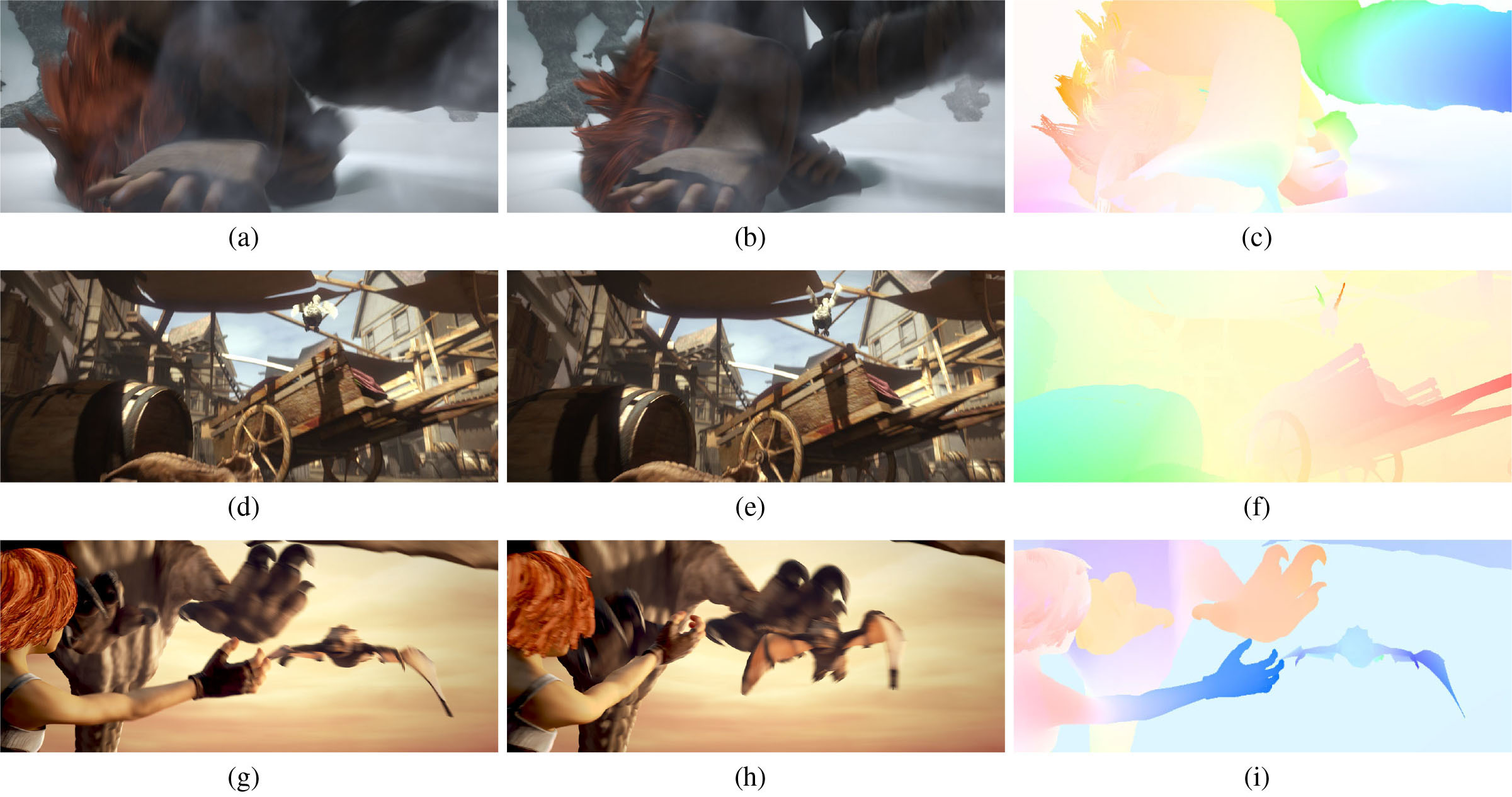

The final data set contains around 1000 images where the optical flow ground truth is available.

3.1 Parameter estimation

For considered metric ( $p=\frac{1}{2},1,2$ , i.e. $\mathcal{L}^{\frac{1}{2}}$ , $\mathcal{L}^{1}$ , $\mathcal{L}^{2}$ , respectively) and color space (sRGB, XYZ, $L^{*}a^{*}b^{*}$ , CMY) we estimated best model parameters using a set of three images with their corresponding depth map (training set) as shown in Fig. 5.

Figure 5.

Training set. The third row shows the location of the sparse depth (yellow points) superimposed to the reference image.

We leave the rest of 997 reference color images and depth ground truth to validate the model.

3.1.1 Estimation using PSO

The AMLE has the following parameters: neighbor size (radius), spatial constant $\kappa_{x}$ and photometric constant $\kappa_{c}$ , iteration number ( $n_{\text{iter}}$ ) were estimated using the PSO algorithm following Eqs (25) and (26). The PSO algorithm minimized the average MAE and MSE for the training set. To estimate the best parameters, we set 50 individuals, 30 iterations. Figure 6 shows learning curves for AMLE and bAMLE using $p=\frac{1}{2}$ and sRGB color space.

Figure 6.

The evolution curve for the PSO. First row shows performance of the PSO algorithm estimation parameter for AMLE for 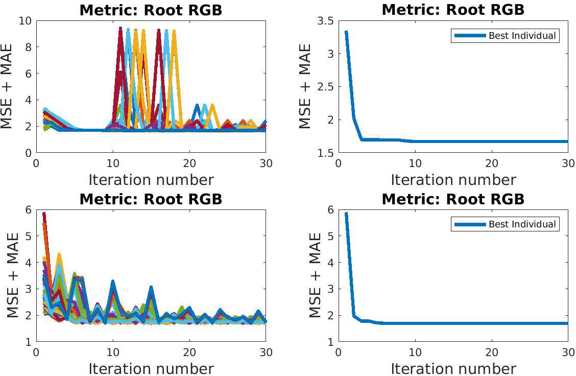$p=\frac{1}{2}$ , sRGB color space. We show to the left the evolution of 50 individuals and the right best individual. Second row shows for $p=\frac{1}{2}$ and sRGB estimating parameters for bAMLE. We show to the left evolution of 50 individuals and the right the best individual.

Figure 7.

Evolution of the EHO algorithm optimizing MSE $+$ MAE.

Table 1 shows the final error for each considered model.

Table 1

MSE $+$ MAE obtained by the PSO algorithm training AMLE using each $\mathcal{L}^{p}$ metric and color space

Metric	sRGB (m)	XYZ (m)	$L^{}a^{}b^{*}$ (m)	CMY (m)
$\mathcal{L}^{\frac{1}{2}}$	1.669	1.663	1.684	1.669
$\mathcal{L}^{1}$	1.709	1.682	1.692	1.733
$\mathcal{L}^{2}$	1.767	1.757	1.686	1.764

Table 2

MSE $+$ MAE obtained by the PSO algorithm training bAMLE for each $\mathcal{L}^{p}$ metric and color space

Metric	sRGB (m)	XYZ (m)	$L^{}a^{}b^{*}$ (m)	CMY (m)
$\mathcal{L}^{\frac{1}{2}}$	1.632	1.693	1.631	1.629
$\mathcal{L}^{1}$	1.737	1.718	1.631	1.718
$\mathcal{L}^{2}$	1.736	1.737	1.632	1.741

For the bAMLE interpolator, we used also the PSO algorithm to estimate its parameters. We show in Table 2 the final performance value of the bAMLE model.

In general, in Table 1 we observe that, best training stage estimation value was obtained for the metric $\mathcal{L}^{\frac{1}{2}}$ . If we compare columns most stable values were obtained using $L^{*}a^{*}b^{*}$ color space for $p=\frac{1}{2}$ , 1 and 2. In Table 1 we present the selected models in bold.

In Table 2 we selected $\mathcal{L}^{\frac{1}{2}}$ , RGB and $L^{*}a^{*}b^{*}$ color space.

3.1.2 Estimation using EHO

Additionally, we have estimated the parameters of the bAMLE model using Elephant Herd Optimization to compare the performance of different parameter estimation methods. Performing this task we considered 5 clans and 10 elephants per clan. We considered $\alpha=$ 0.5 and $\beta=$ 0.95. In Table 3 we show obtained performance final error of the EHO estimation bAMLE Model parameters using $\mathcal{L}^{\frac{1}{2}}$ metric and different color spaces.

Table 3
MSE+MAE obtained by the EHO algorithm training bAMLE for the $\mathcal{L}^{\frac{1}{2}}$ metric and different color spaces

Metric	sRGB (m)	XYZ (m)	$L^{}a^{}b^{*}$ (m)	CMY (m)
$\mathcal{L}^{\frac{1}{2}}$	1.671	1.666	1.677	1.674

Figure 8.

Results obtained by bAMLE model with RGB color space and $\mathcal{L}^{1}$ . (a) sparse depth data. (b) Completed depth data. (c) and (d) two views of the reconstructed 3D scene.

We show in Fig. 7 the evolution of the best individual in each generation in the optimization using 30 iterations, 50 elephants, and 5 clans.

In the first row of Fig. 7 we how the evolution of the EHO algorithm minimizing MSE $+$ MAE for the same training set. We show the evolution using sRGB and XYZ color spaces. In the second row, we show the evolution using $L^{*}a^{*}b^{*}$ and CMY color spaces, observing that the EHO algorithm converges in around 20 iterations.

3.2 Comparison between PSO and EHO

As we see in Tables 2 and 3, comparing the performance of PSO and EHO algorithm, we observe that PSO reaches a bit better performance than the EHO algorithm in most of the color spaces, using the metric $\mathcal{L}^{\frac{1}{2}}$ . In our opinion, in this context, EHO does not contribute with new parameters value. PSO solved the problem correctly.

4. Results of depth completion on KITTI dataset

We show in Table 4 the final results obtained by the selected models in the test KITTI dataset. We have completed 997 incomplete depth maps of the data set.

Table 4
Results obtained by different methods in KITTI depth completion validation set

Method	MSE (m)	MAE (m)
DeepLiDAR [26]	0.687	0.215
bAMLE ( $L^{}a^{}b^{*}+\mathcal{L}^{\frac{1}{2}}$ )	1.737	0.543
bAMLE (sRGB $+\mathcal{L}^{\frac{1}{2}}$ )	1.692	0.457
AMLE ( $L^{}a^{}b^{*}+\mathcal{L}^{\frac{1}{2}}$ )	1.783	0.457
AMLE (sRGB $+\mathcal{L}^{\frac{1}{2}}$ )	1.779	0.4815
CNN [10]	2.100	0.680
Bilateral	2.989	1.201

Table 4 shows that the bAMLE outperforms the AMLE model. The best performance was obtained by bAMLE using sRGB color space and square root value metric. Both methods present a performance in the middle of the KITTI ranking. Methods that present better performance use CNN [26], which are more complex to implement than our proposal and take hours to be trained. Figure 8 shows examples of interpolated depth images using bAMLE model.

AMLE and bAMLE using CMY and $\mathcal{L}^{2}$ present the worst results in the training stage. We didn’t select those models.

Figure 9.

Obtained color-coded optical flow using the model proposed in [25]. (a) Estimated optical for ambush_4 sequence. (b) optical flow market_6 sequence. (c) Optical flow for temple_3 sequence. (d), (e) and (f) are the estimated occlusion-disocclusion for sequence ambush_4, market_6, and temple_3, respectively.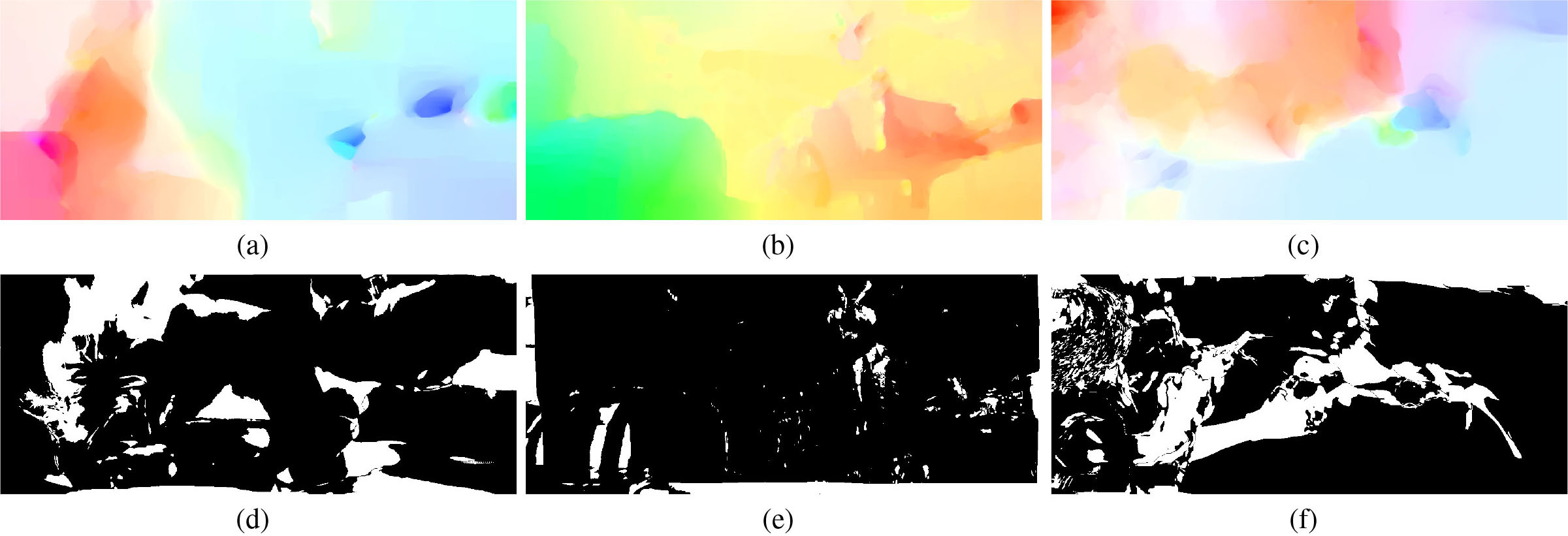

4.1 Median filtering

As the last stage of depth estimation, we filtered the model output $u$ with a median filter to eliminate outliers or noise of the estimation. In Table 5 we show the performance using this filter. In the Table, we recall the results presented in the previous version of this manuscript. We observe that our current version of the algorithm with another metric, other color space, and Median filter outperforms our previous versions in [16]. Our proposal performs better than bilateral filter but worst than DeepLidar [26]. DeepLidar uses CNN, which more complex than our proposal.

Table 5
Results obtained by different methods in the KITTI depth completion validation set

Method	MSE (m)	MAE (m)
DeepLiDAR [26]	0.687	0.215
bAMLE ( $L^{}a^{}b^{*}+\mathcal{L}^{\frac{1}{2}}$ $+$ Median)	1.687	0.577
bAMLE (RGB $+$ $\mathcal{L}^{\frac{1}{2}}$ $+$ Median)	1.643	0.480
bAMLE [16]	1.786	0.440
AMLE [16]	1.801	0.471
CNN [10]	2.100	0.680
Bilateral	2.989	1.201

4.2 Example of a methodology application

Following ideas in [17], we applied the bAMLE to complete optical flow. The optical flow of the video sequence is the displacements of the pixels from the reference image (current image) to the target image (next image). Occluded or disoccluded points can not be matched between two consecutive images. The method in [25] has an occlusion-disocclusion estimator, based on large values of the optical flow estimation error. We detected the occlusion-disocclusion, and we constructed a binary mask with this information, which is used to eliminate the estimated optical flow in those regions. Then, each component of the optical flow is interpolated as in [17] but in our case using bAMLE.

Using the robust optical flow method presented in [25] we estimated the optical flow of the sequences in Fig. 4, and we show the obtained results in Fig. 9.

Using the results presented in Fig. 9 we computed the end-point-error (EPE) and average-angular-error (AAE) for each optimal flow estimation according to the equations:

$\displaystyle\textit{EPE}=\frac{1}{n}\sum_{i=1}^{n}\sqrt{(g_{1i}-u_{1i})^{2}+(% g_{2i}-u_{2i})^{2}}$ $\displaystyle\textit{AAE}=$ (29) $\displaystyle\frac{1}{n}\sum_{i=1}^{n}\cos^{-1}\left(\frac{1+g_{1i}u_{1i}+g_{2% i}u_{2i}}{\sqrt{1+g_{1i}^{2}+g_{2i}^{2}}\sqrt{1+u_{1i}^{2}+u_{2i}^{2}}}\right),$

where $(g_{1i},g_{2i})$ are the horizontal and vertical components of the optical flow ground-truth, $(u_{1i},u_{2i})$ are the two components of the estimated optical flow, and $n$ es the number of point of the optical flow field.

Thus, the obtained EPE and AAE are presented in Table 6.

Table 6

EPE and AAE for video sequences extracted from MPI-Sintel

Sequence	EPE pixels	AAE degrees
ambush_4	42.03	38.84 ${}^{\circ}$
market_6	2.17	5.05 ${}^{\circ}$
temple_3	24.66	45.52 ${}^{\circ}$
Average	22.95	29.80 ${}^{\circ}$

We are taking into account the occlusion-disocclusion mask and the estimated optical flow. We did not consider the values of the estimated optical flow in the occlusion-not occlusion points. We created an artificial hole in each optical flow component, and then we fill in the wholes using bAMLE as an interpolator. We show in Fig. 10 the hole added to the optical flow. In the sequence market_6, the EPE increases from 2.17 to 2.21, 0.04, which is very small. In the other two cases, ambush_4 and temple_3, the EPE drop from 42.03 to 41.92 and from 22.95 to 22.87, respectively.

Figure 10.

Holes added to the optical flow estimation used to show other possible applications of the proposal. The holes are presented in white color (c) Holes added to coded optical flow for sequence ambush_4. (b) Holes added to sequence market_6 sequence. (c) Holes added to sequence temples_6 sequence.

After completing each component of the optical flow, we computed the optical flow estimation error EPE and AAE as we show in Table 7. As we see in Table 7 the average EPE and AAE are inferior to the one obtained by the original algorithm presented in 6.

Table 7

EPE and AAE for the completed video sequence extracted from MPI-Sintel

Sequence	EPE pixels	AAE degrees
ambush_4	41.92	38.46 ${}^{\circ}$
market_6	2.21	5.16 ${}^{\circ}$
temple_3	24.47	44.79 ${}^{\circ}$
Average	22.87	29.47 ${}^{\circ}$

4.3 Discussion

We have evaluated AMLE and bAMLE in the depth completion task for different color spaces and different metrics. We have selected the most frequently used color spaces such as s $R B G$ or $L^{*}a^{*}b^{*}$ to represent color images. In the training stage determining the best AMLE parameter, we show in Table 1 that the best result was obtained by XYZ, color space, the sRGB color space, $L^{*}a^{*}b^{*}$ , and finally CMY. In this stage, we selected sRGB because it is the most traditional, and $L^{*}a^{*}b$ is most stable as the metric changes.

Also, in the training stage, we have compared the performance of the PSO and EHO algorithm estimating parameters. We observed that the EHO method performs similarly to PSO, not showing a notorious improvement in the results. Parameters present some restrictions, for example, the iteration number can not be negative, or neither the $\beta$ parameter could be negative. We observed a tendency performed by EHO to saturate the parameter in minimum feasible values. Thus, we decided to keep using the PSO algorithm in the validation stage.

We tested different metrics giving values to the $p$ exponent in the metric formulation. We tested this three values $p=2$ , $p=1$ , $p=\frac{1}{2}$ and we assessed the model in the KITTI depth completion suite. In the validation set, we show that the best performance was obtained by the combination of $\mathcal{L}^{\frac{1}{2}}$ and sRGB color space. Additionally, the use of the median filter as a post-processing stage helps us to reach better results. The median filter eliminates noise and outliers. A good implementation of a fast median filter can be found in the CUDA toolkit to use for further developments.

We also stated in this manuscript an extension of our proposal to a temporal domain that will be evaluated as future work. The proposal considers the use of a sequence of reference images, a sequence of depth maps, and the optical flow of the video sequence.

Our proposal can be extended to other domains such that optical flow can be a new possibility to be explored in future work. Other possibilities can be to use the proposal as an up-sampling tool in image scale pyramids.

5. Conclusions

We have evaluated our implementation of AMLE and bAMLE in the KITTI depth completion suite, using different metrics and color spaces for the reference image. The combination of a metric based on the square root ( $\mathcal{L}^{\frac{1}{2}}$ ) and the sRGB color space reach the best performance. Surprisingly CIE- $L^{*}a^{*}b^{*}$ color space is robust to the metric changes, and it performs very robustly, not depending on the $p$ value. The implementation of bAMLE is a weighted sum, which is very easy and fast to implement. In future work, we will test the use of the Dijkstra algorithm instead of using an approximation of the distance between points. Also, we will evaluate the extension of this methodology to the completion of depth video sequences numerically.

References

Caselles

Igual

and Sander

, An axiomatic approach to scalar data interpolation on surfaces, Numerische Mathematik 102(3) (2006), 383–411.

Caselles

Morel

J.-M.

and Sbert

, An axiomatic approach to image interpolation, IEEE Transaction on image Processing 7(2) (1998), 376–386.

Aronsson

, Extension of functions satisfyng Lipschitz conditions, Aktiv fuer Mathematik 6(6) (1967), 551–561.

Aronsson

, On the partial differential equation ux2⁢ux⁢x+2⁢ux⁢uy⁢ux⁢y+uy2⁢uy⁢y=0, Aktiv fuer Matematik 7(5) (1968), 395–425.

Huang

J.-B.

Ahuja

and Yang

M.-H.

, Joint image filtering with depth convolutional networks, Transaction on Pattern Analysis and Machine Intelligence 41(8) (2019), 1909–1923. doi: 10.1109/TPAMI.2018.2890623.

Park

Kim

Tai

Y.-W.

Brown

M.S.

and Kweon

, High quality depth map upsampling for 3D-ToF cameras, in: Proceedings of the IEEE International Conference on Computer Vision 2011, 2011, pp. 1623–1630.

Lazcano

Arias

Facciolo

and Caselles

, A gradient based neighborhood filter for disparity interpolation, in: Proceedings of the IEEE International Conference on Image Processing, 2012, pp. 873–876. doi: 10.1109/ICIP.2012.6466999.

Tomasi

and Manduchi

, Bilateral filter for gray and color images, in: Proceedings of the IEEE International Conference on Computer Vision, 1998, pp. 839–846.

Barnes

Anwar

and Zheng

, From depth what can you see? Depth completion via auxiliary image reconstruction, in: Proceedings of the IEEE Conference on Computer Vision and Pattern Recognition (CVPR), 2020.

10.

Uhrig

Schneider

Franke

Brox

and Geiger

, Sparsity invariant CNNs, in: Proceedings of the International Conference on 3D Vision (3DV), 2017.

11.

Imran

Long

Liu

and Morris

, Depth coefficients for depth completion, in: Proceedings of the IEEE Conference on Computer Vision and Pattern Recognition, 2019, pp. 12438–12447.

12.

Lai

W.-S.

Huang

J.-B.

Ahuja

and Yang

M.-H.

, Fast and accurate image super-resolution with deep laplacian pyramid network, Transaction on Pattern Analysis and Machine Intelligence 41(11) (2019), 2599–2613.

13.

Eldesokey

Felsberg

Holmquist

and Persson

, Uncertainty-aware cnns for depth completion: Uncertainty from beginning to End, in: Proceedings of the IEEE Conference on Computer Vision and Pattern Recognition (CVPR), 2020.

14.

Almansa

Cao

Gousseau

and Rougé

, Interpolation of digital elevation models using AMLE and related methods, IEEE Transaction on Geocience and Remote Sensing 40(2) (2002), 314–325.

15.

Oliver

Raad

Ballester

and Haro

, Motion inpainting by an image-based geodesic AMLE method, in: Proceedings of the IEEE International Conference on Image Processing (ICIP), 2018, pp. 2267–2271. doi: 10.1109/ICIP.2018.8451851.

16.

Lazcano

Calderero

and Ballester

, Depth image completion using anisotropic operators, in: Proceedings of the 12th International Conference on Soft Computing and Pattern Recognition (SoCPaR 2020). SoCPaR 2020. Advances in Intelligent Systems and Computing Abraham

et al., eds, 1383 Springer, Cham, (2021).

17.

Raad

Oliver

Ballester

Haro

and Meinhardt

, On anisotropic optical flow inpainting algorithms, Image Processing On Line 10 (2020), 78–104. doi: 10.5201/ipol.2020.281.

18.

Zou

Xiang

Chen

and Qiao

, Simultaneous semantic segmentation and depth completion with constraint of boundary, Sensors 20(3) (2020), 1–25. doi: 10.3390/s20030635. https://www.mdpi.com/1424-8220/20/3/635.

19.

Yao

Roxas

Ishikawa

Ando

Shimamura

and Oishi

, Discontinuous and smooth depth completion with binary anisotropic diffusion tensor, IEEE Robotics and Automation Letters 5(4) (2020), 5128–5135. doi: 10.1109/LRA.2020.3005890.

20.

Bai

Zhao

Elhousni

and Huang

, DepthNet: Real-time LiDAR point cloud depth completion for autonomous vehicles, IEEE Access 8 (2020), 227825–227833. doi: 10.1109/ACCESS.2020.3045681.

21.

Schneider

Pinggera

Franke

Pollefeys

and Stiller

, Semantically guided depth upsampling, in: German Conference on Pattern Recognition, Springer, 2016, pp. 37–48.

22.

Manfredi

J.J.

Oberman

A.M.

and Sviridov

A.P.

, Nonlinear elliptic partial differential equation and p-harmonic functions on graphs, Differential Integral Equations 28(1/2) (2015), 79–102.

23.

Oberman

A.M.

, A convergent difference scheme for the infinity laplacian: Construction of absolutely minimizing lipschitz extensions, Mathematics of Computation 74(251) (2005), 1217–1230.

24.

Kennedy

and Eberhart

, Particle swarm optimization, in: Proceedings of IEEE International Conference on Neural Networks IV, 1995, pp. 1942–1948.

25.

Lazcano

, An empirical study of exhaustive matching for improving motion field estimation, Information 9 (2018), 320.

26.

Qiu

Cui

Zhang

Liu

Zeng

and Pollefeys

, DeepLiDAR: Deep surface normal guided depth prediction for outdoor scene from sparse lidar data and single color image, in: Proceedings of the IEEE Conference on Computer Vision and Pattern Recognition, 2019.

Comparing different metrics on an anisotropic depth completion model

Abstract

Keywords

1. Introduction

1.1 Related works

2.4 Temporal extension

2.5.1 sRGB to XYZ

2.6.1 PSO algorithm

3. Data set and experiments

Table 3 MSE+MAE obtained by the EHO algorithm training bAMLE for the ℒ 1 2 metric and different color spaces

4. Results of depth completion on KITTI dataset

Table 4 Results obtained by different methods in KITTI depth completion validation set

Table 5 Results obtained by different methods in the KITTI depth completion validation set

5. Conclusions

References

Table 3
MSE+MAE obtained by the EHO algorithm training bAMLE for the $\mathcal{L}^{\frac{1}{2}}$ metric and different color spaces

Table 4
Results obtained by different methods in KITTI depth completion validation set

Table 5
Results obtained by different methods in the KITTI depth completion validation set