
Abstract
Distributed Constraint Optimization Problems (DCOPs) have emerged as one of the prominent multi-agent architectures to govern the agents’ autonomous behavior in a cooperative multi-agent system (MAS) where several agents coordinate with each other to optimize a global cost function taking into account their local preferences. They represent a powerful approach to the description and resolution of many practical problems. However, typical MAS applications are characterized by complex dynamics and interactions among a large number of entities, which translate into hard combinatorial problems, posing significant challenges from a computational and coordination standpoints.
This paper reviews two methods to promote a hierarchical parallel model for solving DCOPs, with the aim of improving the performance of the DCOP algorithm. The first is a Multi-Variable Agent (MVA) DCOP decomposition, which exploits co-locality of an agent’s variables allowing the adoption of efficient centralized techniques to solve the subproblem of an agent. The second is the use of Graphics Processing Units (GPUs) to speed up a class of DCOP algorithms.
Finally, exploiting these hierarchical parallel model, the paper presents two critical applications of DCOPs for demand response (DR) program in smart grids. The Multi-agent Economic Dispatch with Demand Response (EDDR), which provides an integrated approach to the economic dispatch and the DR model for power systems, and the Smart Home Device Scheduling (SHDS) problem, that formalizes the device scheduling and coordination problem across multiple smart homes to reduce energy peaks.
Keywords
Introduction
The power network is the largest operating machine on earth, generating more than US$400 billion a year. 1 A significant concern in power networks is for the energy providers to be able to generate enough power to supply the demands at any point in time. Short terms demand peaks are however hard to predict and hard to address while meeting increasingly higher levels of sustainability. Thus, in the modern smart electricity grid, the energy providers can exploit the demand-side flexibility of the consumers to reduce the peaks in load demand.
This control mechanism is called Demand response (DR) and can be obtained by scheduling shiftable loads (i.e., a portion of power consumption that can be moved from a time slot to another) from peak to off-peak hours [17, 42]. Due to concerns about privacy and users’ autonomy, such an approach requires a decentralized, yet, coordinated and cooperative strategy, with the active participation of both the energy providers and consumers.
In a cooperative multi-agent system (MAS) multiple autonomous agents interact to pursue personal goals and to achieve shared objectives. The Distributed Constraint Optimization Problem (DCOP) model [12, 45] is an elegant formalism to describe cooperative multi-agent problems that are distributed in nature and where a collection of agents attempts to optimize a global objective within the confines of localized communication. DCOPs have been applied to solve a variety of coordination and resource allocation problems [22, 48], sensor networks [9], and are shown to be suitable to model various DR programs in the smart grid [16, 36].
DCOP resolution algorithms are classified as either complete or incomplete. Complete algorithms guarantee the computation of an optimal solution to the problem, while incomplete approaches trade optimality for faster runtimes. DCOP algorithms employ one of two broad approaches: distributed search-based techniques [11, 47] or distributed inference-based techniques [9, 41]. In search-based techniques, agents visit the search space by selecting value assignments and communicating them to other agents. Inference-based techniques rely instead on the notion of agent-belief, describing the best cost an agent can achieve for each value assignment of its variables. These beliefs drive the value selection process of the agents to find an optimal solution to the problem.
Despite their success, the adoption of DCOPs on large, complex, instances of problems faces several limitations, including restricting assumptions on the modeling of the problem and the inability of current solvers to capitalize on the presence of structural information.
In this paper, we review a multi-variable-agent (MVA) DCOP decomposition to allow agents to solve complex subproblems efficiently, and a technique to speed up the execution of inference-based algorithms via graphic processing units (GPUs) parallel architectures. These techniques enable us to design practical algorithms to solve large, complex, DCOPs efficiently. We review two DR applications of DCOPs, one where the goal is to optimize the power generator dispatch, while taking into account dispatchable loads, and another in the context of home automation, in which a home agent coordinates the schedule of smart devices to satisfy the user preferences while minimizing the global peaks of energy consumption.
The paper is organized as follows: Section 2 recalls the main definitions and describes two important complete and approximated algorithms for solving DCOPs. Section 3 briefly reviews the GPU programming model. Section 4 describes a decomposition technique that is used for solving DCOPs where each agents is responsible of solving a complex sub-problem. Section 5 describes a DCOPs solving technique that is accelerated through the use of GPUs. Section 6 reviews two complex multi-agent applications of DR that are solved using DCOP techniques. The first application, presented in Section 7, is an approach to optimize demand response at large scale, from a system operator perspective, by acting on large electric generators and loads. The second application, illustrated in Section 8, is an approach to minimize the energy peaks through a demand response program that makes use of automated schedules of smart home devices. Finally, Section 9 concludes the work.
Background: DCOP
Let us start by defining the theoretical framework that is used for modeling smart grid and home automation problems.
Preliminaries
A Distributed Constraint Optimization Problem [12, 45] is a tuple
With a slight abuse of notation, we consider the function
A partial assignment σ
X
is an assignment of values to a set of variables
The cost
Given a DCOP P,
Following [15], we introduce the concepts of local variables for an agent a
i
: For each agent The agent interaction graph For each a
i
, we denote with
A widespread assumption in the communication model of a DCOP algorithm is that each agent can communicate exclusively with its neighboring agents in the agent interaction graph.
A DFS pseudo-tree arrangement of A
P
is a subgraph
Edges of A P that appear in T P are referred to as tree edges,while the remaining edges of A P are referred to as back edges. Fig. 1 (right) shows an example of a pseudo tree for the constraint graph in Fig. 1 (left).
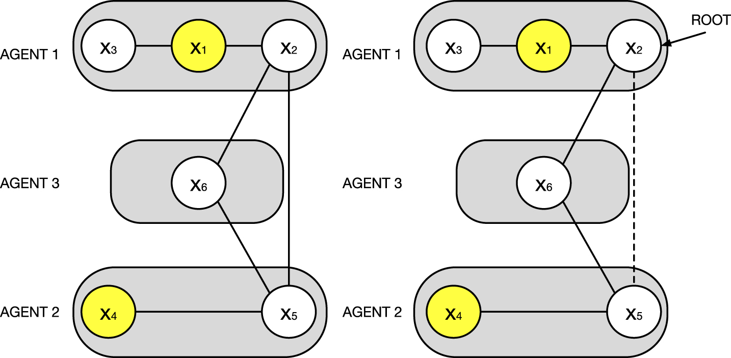
Constraint Graph (left) and Pseudo Tree (right) of the DCOP of Example 1. x2, x5, x6 are the interface variables. Boldface edges are tree edges. {x2, x5} is a back edge.
In the following, we describe two popular DCOP algorithms: a complete inference-based algorithm and an incomplete search-based algorithm. These algorithms were originally proposed in the context in which each agent controls a single variable. We thus restrict our attention to this special case and describe a generalization technique to handle multiple-variable agents in Section 4.
The Distributed Pseudo-tree Optimization Procedure (DPOP) [30] is one of the most popular DCOP resolution algorithms. DPOP is a complete, inference-based algorithm, consisting of three phases.
In the first phase, the variables are ordered through a depth-first search visit of G P into a DFS pseudo-tree. A pseudo-tree construction is achieved through a distributed algorithm (e.g., [1]). A set of variables, called the separator set sep (x i ) is computed for each node x i . sep (x i ) contains all ancestors of x i in the pseudo-tree that are connected with via tree edges or back edges to x i or one of the descendants of x i in the pseudo-tree.
In the second phase, called the UTIL propagation phase, each agent, starting from the leaves of the pseudo-tree executes two operations: (1) It aggregates the costs in its subtree for each value combination of variables in its separator and the variables it controls, and (2) It eliminates the variables it controls by optimizing over the other variables (i.e., for each combination of values for the variables in its separator, it selects the one with the smallest cost). The aggregated costs are encoded in a UTIL message, which is propagated from children to their parents, up to the root.
In the third phase, called the VALUE propagation phase, each agent, starting from the root of the pseudo-tree, selects the optimal value for its variables. The optimal values are calculated based on the UTIL messages received from the children and the VALUE message received from its parent. The VALUE messages contain the optimal values of the variables and are propagated from parents to their children, down to the leaves of the pseudo-tree.
The time and the space complexities of DPOP are dominated by the UTIL propagation phase, which is exponential in the maximum number of variables in a set sep (x i ). The other two phases require a polynomial number of linear sized messages (in the number of variables of the problem), and the complexity of the local operations is at most linear in the size of the domain [30].
MGM
Maximum Gain Message (MGM) [26] is an incomplete, search-based algorithm that performs a distributed local search to solve a DCOP. Each agent a i starts by assigning a random value to each of its variables. The agent then sends this information to all of its neighbors in G P . Upon receiving the values of its neighbors, each agent calculates the maximum gain (i.e., the maximum decrease in cost) if it changes its values and sends this information to all of its neighbors as well. Upon receiving the gains of its neighbors, it changes its values if its gain is the largest among its neighbors. This process is repeated until a termination condition is met. MGM provides no quality guarantees on the returned solution.
Let us indicate with
Background: GPU
Modern Graphics Processing Units (GPUs) are massive parallel architectures, offering thousands of computing cores and a rich memory hierarchy to support graphical processing. NVIDIA’s Compute Unified Device Architecture (CUDA) [37] aims at enabling the use of the multiple cores of a graphics card to accelerate general purpose (non-graphical) applications by providing programming models and APIs that enable the full programmability of the GPU. The computational model supported by CUDA is Single-Instruction Multiple-Threads (SIMT), where multiple threads perform the same operation on multiple data points simultaneously.
A GPU is constituted by a series of Streaming MultiProcessors (SMs), whose number depends on the specific class of GPUs. For example, the Fermi architecture provides 16 SMs, as illustrated in Fig. 2 (left). Each SM contains a number of computing cores, each containing an ALU and a floating-point processing unit. Figure 3 (right) shows a typical CUDA logical architecture. A CUDA program is a C/C++ program that includes parts meant for execution on the CPU (referred to as the host) and parts meant for parallel execution on the GPU (referred as the device). A parallel computation is described by a collection of GPU kernels, where each kernel is a function to be executed by several threads. When mapping a kernel to a specific GPU, CUDA schedules groups of threads (blocks) on the SMs. In turn, each SM partitions the threads within a block in warps 3 for execution, which represents the smallest work unit on the device. Each thread instantiated by a kernel can be identified by a unique, sequential, identifier (T id ), which allows differentiating both the data read by each thread and the code to be executed.

Fermi Hardware Architecture (left) and CUDA Logical Architecture (right).
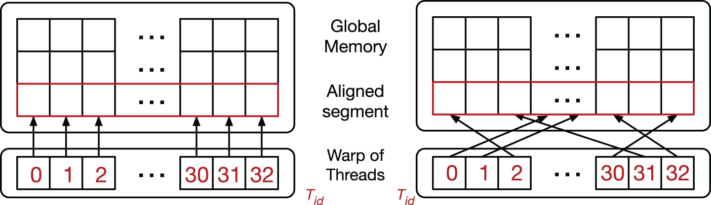
Coalesced (left) and scattered (right) data access patterns.
GPU and CPU are, in general, separate hardware units with physically distinct memory types connected by a system bus. Thus, for the device to execute some computation invoked by the host and to return the results to the caller, a data flow needs to be established from the host memory to the device memory and vice versa. The device memory architecture is entirely different from that of the host, in that it is organized in several levels differing to each other for both physical and logical characteristics.
Each thread can utilize a small number of registers, 4 which have thread lifetime and visibility. Threads in a block can communicate by reading and by writing a common area of memory, called shared memory. The total amount of shared memory per block is typically 48KB. Communication between blocks and communication between the blocks and the host is achieved through a large global memory. The data stored in the global memory has global visibility and lifetime. Thus, it is visible to all threads within the application (including the host) and lasts for the duration of the host allocation.
Apart from lifetime and visibility, different memory types have also different dimensions, bandwidths, and access times. Registers have the fastest access memory, typically consuming within a clock cycle per instruction, while the global memory is the slowest but largest memory accessible by the device, with access times ranging from 300 to 600 clock cycles. The shared memory is partitioned into 32 logical banks, each serving exactly one request per cycle. Shared memory has a minimal access latency, provided that multiple thread memory accesses are mapped to different memory banks.
Bottlenecks and Common Optimization Practices
While it is relatively simple to develop correct GPU programs (e.g., by incrementally modifying an existing sequential program), it is nevertheless challenging to design an efficient solution. Several factors are critical to gaining performance. In this section, we discuss a few common practices that are important for the design of efficient CUDA programs.
Memory bandwidth is widely considered to be a critical bottleneck in the performance of GPU applications. Accessing global memory is relatively slow compared to accessing the shared memory in a CUDA kernel. However, even if not cached, global accesses that cover a segment of 128 contiguous Bytes data are fetched at once. Thus, most of the global memory access latency can be hidden if the GPU kernel employs a coalesced memory access pattern. Figure 3 (left) illustrates an example of coalesced memory access pattern, in which aligned threads in a warp accesses aligned entries in a memory segment, which results in a single transaction. Thus, coalesced memory accesses allow the device to reduce the number of fetches to global memory for every thread in a warp. In contrast, when threads adopt a scattered data accesses (Fig. 3 (right)), the device serializes the memory transaction, drastically increasing its access latency.
Data transfers between the host and device memory are performed through a system bus, which translates to slow transactions. In general, it is convenient to store the data in the device memory. Additionally, batching small memory transfers into a large one will reduce most of the per-transfer processing overhead [37].
The organization of the data in data structures and data access patterns plays a fundamental role in the efficiency of the GPU computations. Due to the computational model employed by the GPU, it is important that each thread in a warp executes the same branch of execution. When this condition is not satisfied (e.g., two threads execute different branches of a conditional construct), the degree of concurrency typically decreases, as the execution of threads performing separate control flows has to be serialized. This is referred to as branch divergence, a phenomenon that has been intensely analyzed within the High Performance Computing (HPC) community [6, 19].
The line of work in this paper focused on using GPUs to improve the performance of DCOP solvers, extends recent approaches to make use of GPUs to enhance performance of constraint solvers [4, 14].
DCOP Applications Challenge: Agents with Multiple Variables
The vast majority of the DCOP resolution algorithms have been proposed in a restrictive setting, in which each agent controls exactly one variable. While this assumption simplifies the algorithm description and its development, it does not hold in many of the applications of our interest. For instance, micro-grids are self-sustainable and autonomous organizations composed of generators and loads within an electric smart grid; this can be modeled as agents whose variables represent the amount of energy to dispatch, transmit, and withdraw from the grid. In a smart home, multiple devices can be coordinated by a single autonomous home assistant, which, too, has to control a large number of variables.
There are two commonly used reformulation techniques to cope with DCOP in which agents control multiple variables [3, 46]: (i) Compilation, where each agent creates a new pseudo-variable, whose domain is the Cartesian product of the domains of all variables of the agent; and (ii) Decomposition, where each agent creates a pseudo-agent for each of its variables. While both techniques are relatively simple, they can be inefficient. In compilation, the memory requirement for each agent grows exponentially with the number of variables that it controls. In decomposition, the DCOP algorithms will treat two pseudo-agents as independent entities, resulting in unnecessary computation and communication costs.
To overcome these limitations, the following subsections discusses the Multi-Variable Agent (MVA) DCOP decomposition, originally proposed in [15]. It enables a separation between the agents’ local subproblems, which can be solved independently using centralized solvers, and the DCOP global problem, which requires coordination of the agents. The decomposition does not lead to any additional privacy loss and enables the use of different centralized and distributed solvers in a hierarchical and parallel fashion.
The MVA Framework
In the MVA decomposition, a DCOP problem P is decomposed into
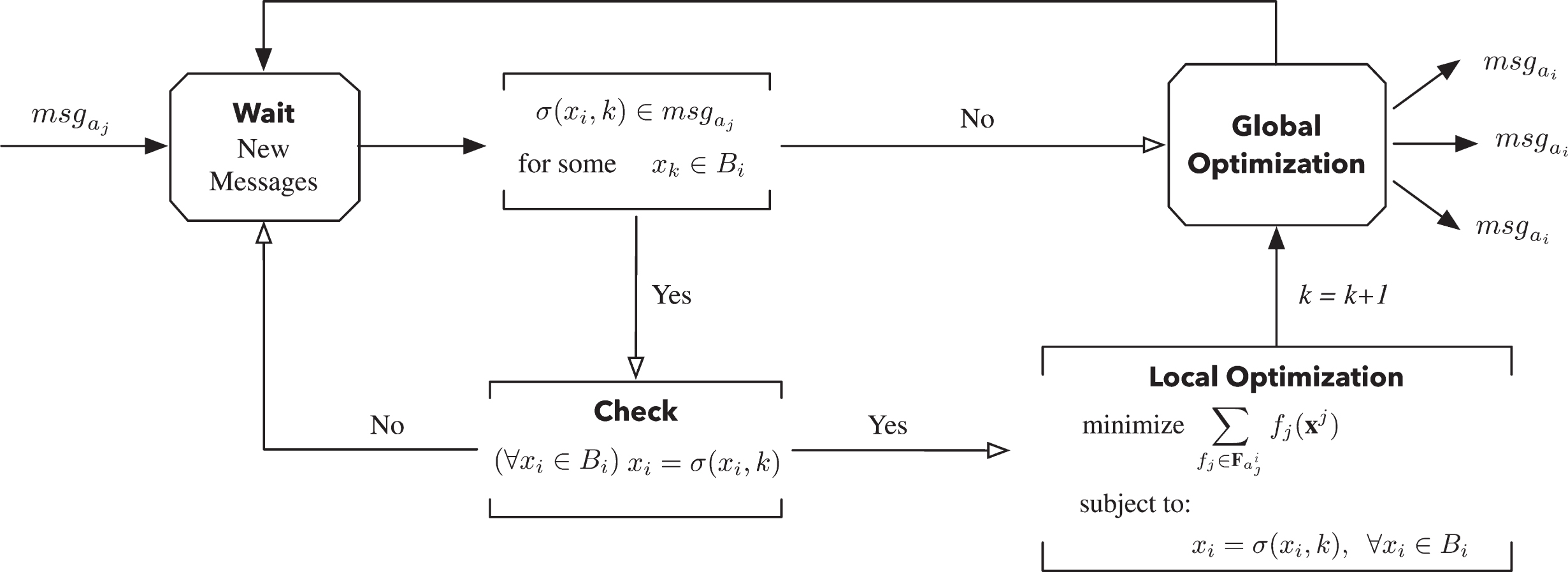
MVA Execution Flow Chart.
Figure 4 shows a flowchart illustrating the four conceptual phases in the execution of the MVA framework for each agent a i :
Phase 1—Wait: The agent waits for a message to arrive. If the received message results in a new value assignment σ (x
r
, k) for an interface variable x
r
of B
i
, then the agent will proceed to Phase 2. If not, it will proceed to Phase 4. The value
Phase 2—Check: The agent checks if it has performed a new complete assignment for all its interface variables, indexed with
Phase 3—Local Optimization: When a complete assignment is given, the agent passes the control to a local solver, which solves the following problem:
Phase 4—Global Optimization: The agent processes the new assignment as established by the DCOP algorithm P G , executes the necessary communications and returns to Phase 1. The agents can execute these phases independently of one another because they exploit the co-locality of their local variables without any additional privacy loss, which is a fundamental aspect of DCOPs [18].
In addition, the local optimization process can operate on m ≥ 1 combinations of value assignments of the interface variables, before passing control to the next phase. This is the case when the agent explores m different assignments for its interface variables in Phases 2 and 3. These operations are performed by storing the best local solution and their corresponding costs in a cost table of size m, which can be visualized as a cache memory. The minimum value of m depends on the choice of the global DCOP algorithm P G . For example, for common search-based algorithms such as asynchronous forward-bounding (AFB), it is 1, while for common inference-based algorithms such as DPOP, it is exponential in size of the separator set.
Correctness, completeness, asymptotical complexity, and an extensive evaluation of the MVA decomposition are presented in [15].
As mentioned in Section 2.2, the aggregation and elimination operations within the UTIL propagation phase of DPOP are the most expensive operations of the algorithm. In this section, we review the GPU-based Distributed Bucket Elimination (GpuBE) framework [13], which extends DPOP by exploiting GPU parallelism within the aggregation and elimination (i.e., UTIL) operations to speed up these operations. The key observation that allows us to parallelize these operations is that the computation of the cost for each value combination in a UTIL message is independent of the computation of the other combinations. The use of a GPU architecture allows us to exploit such independence, by concurrently exploring several value combinations of the UTIL message, computed by the aggregation operator, as well as concurrently eliminating variables.
GPU Data Structures
To fully utilize the parallel computational power of GPUs, the data structures need to be designed in such a way to limit the amount of information exchanged between the CPU host and the GPU device, minimizing the accesses to the slow device global memory while ensuring that the data access pattern enforced is coalesced. To do so, we store in the device global memory exclusively the minimal information required to compute the UTIL functions, which are communicated to the GPU once at the beginning of the computation. This allows the GPU kernels to communicate with the CPU host exclusively to exchange the results of the aggregation and elimination processes.
We introduce the following concept: An UTIL-table is a 4-tuple, T = 〈
χ is a list of length | ≺ denotes an ordering relation used to sort the variables in the list
As a technical note, a UTIL-table T is mapped onto the GPU device to store exclusively the cost values χ, not the associated variables values. We assume that the rows of
GPU-based Constraint Aggregation
The constraint aggregation takes as input two UTIL-tables: T i and T o , and aggregates the cost values in χ i to those of χ o for all the corresponding assignments of the shared variables in the scope of the two UTIL-tables. We refer to T i and T o as to the input and output UTIL-tables, respectively.
Consider the example in Fig. 5, the cost values χ i of the input UTIL-table T i (left) are aggregated to the cost values χ o of the output UTIL-table T o (right)—which were initialized to 0. The rows of the two tables with identical value assignments for the shared variables x2 and x3 are shaded with the same color.

Example of aggregation of two tables on GPU.
To optimize the performance of the GPU operations and to avoid unnecessary data transfers to/from the GPU global memory, we only transfer the list of cost values χ for each UTIL-table that needs to be aggregated and employ a simple, perfect hashing function to efficiently associate row numbers with variables’ values. This allows us to compute the indexes of the cost vector of the input UTIL-table relying exclusively on the information of the thread ID and, thus, avoid accessing the scope
To exploit the highest degree of parallelism offered by the GPU device, we: map one GPU thread T
id
to one element of the output UTIL-table, and adopt the ordering relation ≺
T
for each input and output UTIL-table processed.
Adopting such techniques allows each thread to be responsible for performing exactly two reads and one write from/to the GPU global memory. Additionally, the ordering relation enforced on the UTIL-tables allows us to exploit the locality of data and to encourage coalesced data accesses. As illustrated in Fig. 5, this paradigm allows threads (whose IDs are identified in red by their T
id
’s) to operate on contiguous chunks of data. Thus, it minimizes the number of actual read (from the input UTIL-table, on the left) and write (onto the output UTIL-table, on the right) operations from/to the global memory performed by a group of threads with a single data transaction.
5
As a technical detail, the UTIL-tables are created and processed so that the variables in their scope are sorted according to the order ≺ T . This means that the variables with the highest priority appear first in the scope list, while the variables to be eliminated always appear last. Such detail allows us to efficiently encode the elimination operation on the GPU, as explained next.
The variable elimination takes as input a UTIL-table T
o
and a variable x
i
∈

Example of variable elimination on GPU.
The variable elimination is executed in parallel by a number of GPU threads equal to the number of rows of the output UTIL-table. Each thread identifies its row index r o within the output UTIL-table cost values χ o , given its thread ID. It hence retrieves an input row index r j to the value of the first χ o input UTIL-table row to analyze. Note that, as the variable to eliminate is listed last in the scope of the UTIL-table, it is possible to retrieve each unique assignment for the projected output bucket table, simply by offsetting r o by the size of D x i . Additionally, all elements listed in χ o [r j ] , …, χ o [r j + |D x i |] differ exclusively on the value assignment to the variable x i (see Fig. 6). Thus, the GPU kernel evaluates the input UTIL-table cost values associated to each element in the domain of x i , by incrementing the row index r j , |D x i |-1 times, and chooses the minimum cost value. At last, it saves the best cost found to the associated output row.
Note that each thread reads |D x i | adjacent values of the vector χ o , and writes one value in the same vector. Thus, this algorithm (1) perfectly fits the SIMT paradigm, (2) minimizes the accesses to the global memory as it encourages a coalesced data access pattern, and (3) uses a relatively small amount of global memory, as it recycles the memory area allocated for the input UTIL-table, to output the cost values for the output UTIL-table.
For additional details on these operations, and on the theoretical and experimental results of the GPU parallel version of DPDOP, we refer the reader to [13].
With the growing complexity of the current power grid, there is an increasing need for intelligent operations coordinating energy supply and demand. A key feature of the smart grid vision is that intelligent mechanisms will coordinate the production, transmission, and consumption of energy in a distributed way, guaranteeing sustainability, reliability, and resilience. The distributed nature of the grid makes cooperative multi-agent based solutions a natural fit. A critical problem in this domain is that of minimizing the peak load demands, as these are expensive from both a system operational perspective and for the risk associated with power failure due to overload. Demand response (DR) strategies allow customers to make autonomous decisions on their energy consumption and have been shown to improve various power system operations, including load balancing and frequency regulation. From a large scale, power generation perspective, the economic dispatch (ED) of power generators is applied to allocate the power to be produced by each generator minimizing the production costs while satisfying the physical constraints of the power system. Demand response programs enable customers to make informed decisions regarding their energy consumption and can be used to reduce the total peak demand, reshape the demand profile, and thus increase grid sustainability. Maintaining a constant balance between generation and consumption of power is critical for effective power system operations. Section 7 proposes a proactive DCOP approach to the economic dispatch which includes demand response and can quickly respond to the dynamic changes of the grid loads (within a few minutes).
At a smaller scale, from a consumer perspective, demand response can be used to reduce the residential electricity spending by designing smart buildings capable of making autonomous decisions to control power loads, production, and transmission. Through the proliferation of smart devices (e.g., smart thermostats, smart washers) in our homes and offices, the buildings’ automation within the broader smart grid is becoming crucial. Home automation is defined as the automated control of the buildings electrical devices with the objective of the improved comfort of the occupants, improved energy efficiency, and reduced operational costs. Section 8 focuses on the scheduling of smart devices in a decentralized way. In the proposed model, each household is responsible for the schedule of the devices in her building under the assumption that each user has personal preferences and comforts levels. The DR model enables users to act cooperatively to reduce the global energy peaks.
Multi-agent Economic Dispatch with Demand Response (EDDR)
In traditional operations, ED and DR are implemented separately, despite the strong inter-dependencies between these two problems. Fioretto et al. [17] proposed an integrated approach to solve the ED and DR problems to simultaneously maximize the benefits of customers and minimize the generation costs. We survey such approach next.
The EDDR Model
A power grid can be viewed as a network of nodes (called buses in the power systems literature) that are connected by distribution cables and whose loads are served by (electromechanical) power generators. Typically, a group of such power generators is located in a single power station, and a number of power stations are distributed in different geographic areas. Such a power grid can be visualized as an undirected graph
An n-bus power system is considered where each bus injects and withdraws power through a generator
We model each bus as an agent, capable of making autonomous decisions on its power consumption and generation. We assume that there is exactly one generator and one load in each bus. The case with multiple loads and generators per bus can be easily transformed into this simpler model by precomputing the best operational conditions for each output combination of loads and generation power. In other words, each amount p of power that can be injected by the aggregated action of the generators within a bus will take cost c p . The latter, is the value minimizing the sum of the costs of the individual generators when their aggregated power injected equals p. The cost for the aggregated loads at a bus-level follows a similar procedure.
When a load difference is revealed to the power system, the ED problem is to regulate the output of the appropriate units so that the new generation output meets the new load and the generators are at economic dispatch (i.e., they are running efficiently according to some objective function). Near real-time power consumption monitoring from smart meters allows short-term load prediction, which can supply the smart grid with predictions on power consumption levels.
DR resources can be planned to be dispatched at different time scales, from supporting frequency regulation (requiring DR loads to respond in the order of few seconds) to correcting phase imbalance on the feeders (which requires responses in intervals of several minutes) and supporting cold load operations by restraining load demand—every several minutes to an hour intervals. The D-EDDR problem with a time horizon H is presented in [17].
Due to a rippling effect on the generators’ power-cost curve, the generators’ cost functions contain nonlinear terms, which makes the optimization problem non-convex. Additionally, due to the non-linearity of the transmission lines capacity constraints, Fioretto et al., consider a relaxation of the D-EDDR problem in which the transmission lines capacities constraints are modeled as soft constraints with a penalty on the degree of their violation. This approach is similar to the one used by researchers in the power systems community [39, 43].
The D-EDDR problem has been modeled as a Dynamic DCOP [31], which is a sequence of DCOPs 〈P1, P2, … 〉, where each P
t
is associated with a particular time step t. Each DCOP P
t
in the Dynamic DCOP has the same agents
R-Deeds
The Relaxed Distributed Efficient ED with DR Solver (R-
The first and last phases of R- If none of the values in its UTIL-table satisfies all the constraints, it suggests that the problem is insufficiently relaxed. Thus, it increases a parameter ω by a factor of 2 based on the difference with respect to its value in the last iteration,
6
propagates this information to all agents and informs them to reinitialize their UTIL tables with the new updated ω, and solve the new relaxed problem in a new iteration. If there is a row satisfying all the constraints, then the problem may be overly relaxed. Thus, it decreases ω by a factor of 2 based on the difference with respect to its value in the last iteration, and this new relaxed problem is solved in a new iteration.
This process repeats itself until some criteria is met (e.g., a maximum number of iterations, convergence in the solution).
A number of the operations of the algorithm can be sped up through parallelization using GPUs. In particular, the initialization and consistency checks of the different rows of the UTIL-table can be done independently from each other. Additionally, the aggregation of the different rows of the UTIL-tables can also be computed in parallel, fitting well the SIMT processing paradigm. Thus, R-
Empirical Evaluation
We evaluate the proposed algorithms on 5 standard IEEE Bus Systems, 7 all having non-convex solution spaces, and ranging from 5 to 118 buses.
All the generators are set with a 5MW ramp rate limit. We use a 1MW discretization unit for each load and generators. Thus, the maximum domain sizes of the variables are between 100 and 320 in every experiment. The horizon H is set to 12, with each step defining a one hour interval. Additionally, we define a parameter H
opt
that denotes the number of time steps that are considered by R-
We generate 30 instances for each test case. The performance of the algorithms are evaluated using the simulated runtime metric [38], and we imposed a timeout of 5 hours. Results are averaged over all instances. These experiments are performed on a AMD Opteron 6276, 2.3GHz, 128GB of RAM, which is equipped with a GeForce GTX TITAN GPU device with 6GB of global memory. If an instance cannot be completed, it is due to runtime limits for the CPU implementation of the algorithm, and memory limits for the GPU implementation. We set the number of iterations to 10.
We do not report evaluation against existing (Dynamic) DCOP algorithms as the standard (Dynamic) DCOP models cannot fully capture the complexities of the D-EDDR problem (e.g., environment variables with continuous values).
Table 1 tabulates the runtimes in seconds of R- The solution quality increases as H
opt
increases. For the smaller test case with H
opt
= 1, the CPU implementation is faster than the GPU one. However, for all other configurations, the GPU implementation is much faster than its CPU counterpart, with speedups up to 130 times. The reported speedup increase with increasing complexity of the problem (i.e., bus size and H
opt
). The GPU implementation scales better than the CPU implementation. The latter could not solve any of the instances for the configurations with H
opt
= 3 for the 14-bus system and H
opt
= 2 for the 57-bus system. We observe that the algorithms report satisfiable instances within the first four iterations of the iterative process. R-
To validate the solutions returned by R-

Dynamic Simulation of the IEEE 30 Bus with heavy loads.
In our experiment, the first 60 seconds of the simulation are tested enforcing the ED solution in a full load scenario (100% of full load) using the same setting as in [24]. The rest of the simulation deploys the D-EDDR solution returned by R-
While the resolution of the simulation is in microseconds, R-
Residential and commercial buildings are progressively being automated through the introduction of smart devices (e.g., smart thermostats, circulator heating, washing machines). Besides, a variety of smart plugs, which allow users to control devices by remotely switching them on and off intelligently, are now commercially available. Device scheduling can, therefore, be executed by users, without the control of a centralized authority. This schema can be used for demand-side management in a DR program. However, uncoordinated scheduling may be detrimental to DR performance without reducing peak load demands [40]. For an effective DR, a coordinated device scheduling within a neighborhood of buildings is necessary. Privacy concerns arise when users share resources or cooperate to find suitable schedules. This section surveys the Smart Home Device Scheduling (SHDS) problem, which formalizes the problem of coordinating smart devices schedules across multiple smart homes as a multi-agent system, presented initially in [16].
The Problem
A Smart Home Device Scheduling (SHDS) problem is defined by the tuple
H is the planning horizon of the problem, and
Finally, Ω
p
is used to denote the set of all possible states for state property p ∈
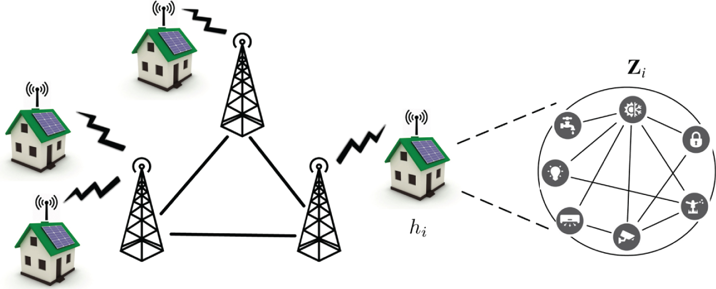
Illustration of a Neighborhood of Smart Homes.
For each home h
i
∈
A tuple
Device Schedules
To control the energy profile of a smart home, we need to describe the behavior of the smart devices acting in the smart home during the time horizon. We formalize this concept with the notion of device schedules. We use
A schedule
Consider the illustration of Fig. 9. The top row shows a possible schedule 〈R, R, C, C, R, R, C, R〉 for a vacuum cleaning robot starting at time 1400 hrs, where each time step is 30 minutes. The robot’s actions at each time step are shown in the colored boxes with letters in them: red with ‘S’ for
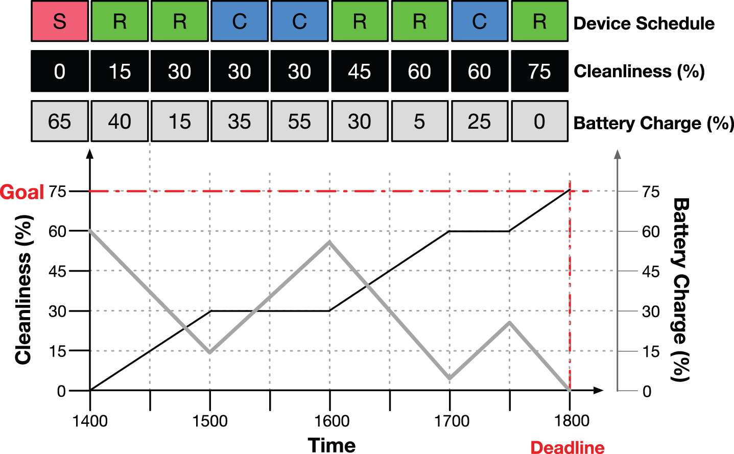
Smart Home Device Scheduling Example.
At a high level, the goal of the SHDS problem is to find a schedule for each of the devices in every smart home that achieves some user-defined objectives (e.g., the home is at a particular temperature within a time window, the home is at a particular cleanliness level by some deadline) that may be personalized for each home. We refer to these objectives as scheduling rules.
The SHDS introduces two types of scheduling rules: Active Scheduling Rules (ASRs) that define user-defined objectives on a desired state of the home (e.g., the living room is cleaned by 1800 hrs). Passive Scheduling Rules (PSRs) that define implicit constraints on devices that must hold at all times (e.g., the battery charge on a vacuum cleaning robot is always between 0% and 100%).
Each scheduling rule indicates a goal state at a home location or on a device ℓ
R
p
∈
Each rule is associated with a set of actuators Φ
p
⊆
Feasibility of Schedules
To ensure that a goal state can be achieved across the desired time window, the system uses a predictive model of the various state properties. This predictive model captures the evolution of a state property over time and how this state property is affected by a given joint action of the relevant actuators.
A predictive model Γ p for a state property p is a function Γ p : Ω p ×× z∈Φ p A z ∪ {⊥} → Ω p ∪ {⊥}, where ⊥ denotes an infeasible state and ⊥+ (·) = ⊥.
In other words, the model describes the transition of state property p from state ω
p
∈ Ω
p
at time step t to time step t + 1 when it is affected by a set of actuators Φ
p
running joint actions
We assume here, without loss of generality, that the state of properties is numeric—when this is not the case, a mapping of the possible states to a numeric representation can be easily defined.
The predictive model of the example above models a device state property. Notice that a recursive invocation of a predictive model allows us to predict the trajectory of a state property p for future time steps, given a schedule of actions of the relevant actuators Φ p .
Given a state property p, its current state ω
p
at time step t
a
, and a schedule
Consider the device scheduling example in Fig. 9. The predicted state trajectories of the charge and cleanliness state properties are shown in the second and third rows. These trajectories are predicted given that the vacuum cleaning robot will take on the schedule shown in the first row of the figure. The predicted trajectories of these state properties are also illustrated in the graph, where the dark gray line shows the states for the robot’s battery charge and the black line shows the states for the cleanliness of the room.
Notice that, to verify if a schedule satisfies a scheduling rule, it is sufficient to check that the predicted state trajectories are within the set of feasible state trajectories of that rule. Additionally, notice that each active and passive scheduling rule defines a set of feasible state trajectories. For example, the active scheduling rule of Example 3 allows all possible state trajectories as long as the state at time step 1800 is no smaller than 75. We use R p [t] ⊆ Ω p to denote the set of states that are feasible according to rule R p of state property p at time step t.
More formally, a schedule
A schedule is feasible if it satisfies all the passive and active scheduling rules of each home in the SHDS problem.
Cost of Schedules
In addition to finding feasible schedules, the goal in the SHDS problem is to optimize for the aggregated total cost of energy consumed.
Each action ξ ∈ A
z
of device z ∈
The objective of an SHDS problem is that of minimizing the following weighted bi-objective function:
Finally, constraint (3) defines the valid trajectories for each scheduling rule r ∈
A DCOP mapping of the SHDS problem is as follows: For each actuator z ∈ An auxiliary interface variable Local soft constraints (i.e., constraints that involve only variables controlled by one agent) whose costs correspond to the weighted summation of monetary costs, as defined in Equation (1). Local hard constraints that enforce Constraint (3). Feasible schedules incur a cost of 0 while infeasible schedules incur a cost of ∞. Global soft constraints (i.e., constraints that involve variables controlled by different agents) whose costs correspond to the peak energy consumption, as defined in the second term in Equation (2).
The neighbors Nai of agent ai are defined as all the agents in the coalition ℋ that contains hi.
MVA-based MGM
The SHDS problem requires several homes to solve a complex scheduling subproblem, which involves multiple variables, and to optimize the resulting energy profiles among the neighborhood of homes. The problem can be thought of as each agent solving a local complex subproblem, whose optimization is influenced by the energy profiles of the agent’s neighbors, and by a coordination algorithm that allows agents to exchange their newly computed energy profiles. We thus adopt the multiple-variable agent (MVA) decomposition [15] to delegate the resolution of the agent’s local problem to a centralized solver while managing inter-agent coordination through a message-passing procedure similar to that operated by MGM, described in Section 2.3. The resulting algorithm is called Smart Home MGM (SH-MGM). SH-MGM is a distributed algorithm that operates in synchronous cycles. The algorithm first finds a feasible DCOP solution and then iteratively improves it, at each cycle, until convergence or time out. We leave the details out and refer the interested reader to [16].
Empirical Evaluation
Our empirical evaluations compare the SH-MGM algorithm against an uncoordinated greedy approach, where each agent computes a feasible schedule for its home devices without optimizing over its cost and the aggregated peak energy incurred.
Each agent controls nine smart actuators to schedule—Kenmore oven and dishwasher, GE clothes washer and dryer, iRobot vacuum cleaner, Tesla electric vehicle, LG air conditioner, Bryant heat pump, and American water heater—and five sensors. We selected these devices as they can be available in a typical (smart) home and they have published statistics (e.g., energy consumption profiles). The algorithms take as inputs a list of smart devices to schedule as well as their associated scheduling rules and the real-time pricing scheme adopted. Each device has an associated active scheduling rule that is randomly generated for each agent and a number of passive rules that must always hold. To find local schedules at each SH-MGM iteration, each agent uses a Constraint Programming solver 8 as a subroutine. An extended description of the smart device properties, the structural parameters (i.e., size, material, heat loss) of the homes, and the predictive models for the homes and devices state properties is reported in [21]. Finally, we set H = 12 and adopted a pricing scheme used by the Pacific Gas & Electric Co. for its customers in parts of California, 9 which accounts for seven tiers ranging from $0.198 per kWh to $0.849 per kWh.
In our first experiment, we implemented the algorithm on an actual distributed system of Raspberry Pis. A Raspberry Pi (called “PI” for short) is a bare-bone single-board computer with limited computation and storage capabilities. We used Raspberry Pi 2 Model B with quadcore 900MHz CPU and 1GB of RAM. We implemented the SH-MGM algorithm using the Java Agent Development Environment (JADE) framework, 10 which provides agent abstractions and peer-to-peer agent communication based on asynchronous message passing. Each PI implements the logic for one agent, and the agent’s communication is supported through JADE and using a wired network connected to a router.
We set up our experiments with seven PIs, each controlling the nine smart actuators and five sensors described above. All agents belong to the same coalition. We set the equal weights α c and α e of the objective (see Equation (2)) to 0.5. Figure 10 (left) illustrates the results of this experiment, where we imposed a 60 seconds timeout for the CP solver. As expected, the SH-MGM solution improves with increasing number of cycles, providing an economic advantage for the users as well as peak energy reduction, when compared to the uncoordinated schema. These results, thus, show the feasibility of using a local search-based schema implemented on hardware with limited storage and processing power to solve a complex problem.
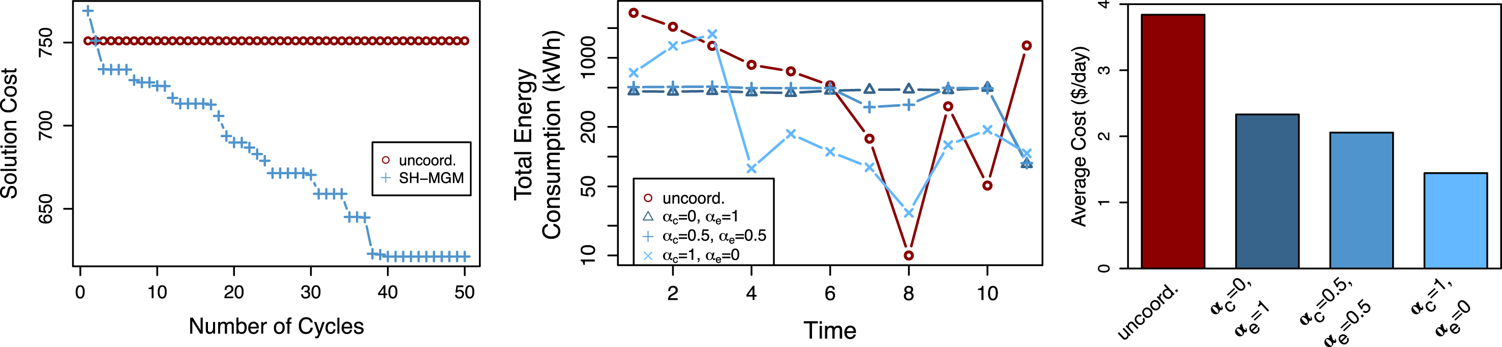
Physical Experimental Result with PIs (left); Synthetic Experimental Results Varying α c and α e (middle and right).
In our second set of experiments, we generate synthetic microgrid instances sampling neighborhoods in three cities in the United States (Des Moines, IA; Boston, MA; and San Francisco, CA) and estimate the density of houses in each city. The average density (in houses per square kilometers) is 718 in Des Moines, 1357 in Boston, and 3766 in San Francisco. For each city, we created a 200m × 200m grid, where the distance between intersections is 20m, and randomly placed houses in this grid until the density is the same as the sampled density. We then divided the city into k(= |ℋ|) coalitions, where each home can communicate with all homes in its coalition. In generating our SHDS topologies, we verified that the resulting topology is connected. Finally, we ensure that there are no disjoint coalitions; this is analogous to the fact that microgrids are all connected to each other via the main power grid.
In these experiments, we imposed a 10 seconds timeout for the agents’ CP solver. We first evaluate the effects of the weights αc and αe (see Equation (2)) on the quality of solutions found by the algorithms. We evaluate three configurations: (αc = 1.0, α e = 0.0), (α c = 0.5, α e = 0.5), and (α c = 0.0, α e = 1.0), using randomly generated microgrids with the density of Des Moines, IA. Figure 10 (middle) shows the total energy consumption per hour (in kWh) of the day under each configuration. Figure 10 (right) illustrates the average daily cost paid by one household under the different objective weights. The uncoordinated greedy approach achieves the worst performance, with the highest energy peak at 2852 kWh and the most expensive daily cost ($3.84). The configuration that disregards the local cost reduction (α c = 0) reports the best energy peak reduction (peak at 461 kWh) but highest daily cost among the coordinated configurations ($2.31). On the other extreme, the configuration that disregards the global peak reduction (α p = 0) reports the worst energy peak reduction (peak at 1738 kWh) but the lowest daily cost among the coordinated configurations ($1.44). Finally, the configuration with α c = α e = 0.5 reports intermediate results, with the highest peak at 539 kWh and a daily cost of $2.18.
For a more extensive analysis of the results, we refer the reader to [16].
Responding to the recent call to action for AI researchers to contribute towards the smart grid vision [32], this paper presented two important applications of Distributed Constraint Optimization Problems (DCOPs) for demand response (DR) programs in smart grids. The multi-agent Economic Dispatch with Demand Response (EDDR) provides an integrated approach to the economic dispatch and the DR model for power systems. The Smart Home Device Scheduling (SHDS) problem formalizes the device scheduling and coordination problem across multiple smart homes to reduce the energy peaks.
Due to the complexity of the problems the adoption of off-the-shelf DCOPs resolutions algorithms is infeasible. Thus, the paper introduces a methodology to exploit the structural problem decomposition (called MVA) for DCOPs, which enables agents to solve complex local sub-problems efficiently. It further discusses a general GPU parallelization schema for inference-based DCOP algorithms, which produces speed-ups of up to 2 order of magnitude.
In the context of EDDR applications, evaluations on a state-of-the-art power systems simulator show that the solutions found are stable within acceptable frequency deviations. In the context of home automation, the proposed algorithm was deployed on a distributed system of Raspberry Pis, each capable of controlling and scheduling smart devices through hardware interfaces. The experimental results show that this algorithm outperforms a simple uncoordinated solution on realistic small-scale experiments as well as large-scale synthetic experiments.
Therefore, this work continues to pave the bridge between the AI and power systems communities, highlighting the strengths and applicability of AI techniques in solving power system problems.
Footnotes
1
Source: U.S. Energy Information Administration.
2
℘ (S) is the power set of a set S.
3
A warp is typically composed of 32 threads.
4
In modern devices, each SM allots 64KB for registers space.
5
Accesses to the GPU global memory are cached into cache lines of 128 Bytes, and can be fetched by all requiring threads in a warp.
6
The larger the value of ω, the more relaxed the problem. The relaxed problem is identical to the original one if ω = 0.
Acknowledgments
We would like to thank all the friends that have worked with us in this challenging research area, namely, Federico Campeotto, Alessandro Dal Palù, Rina Dechter, Khoi D. Hoang, Ping Hou, William Kluegel, Muhammad Aamir Iqbal, Tiep Le, Tran Cao Son, Athena M. Tabakhi, Makoto Yokoo, Roie Zivan, and, in particular, William Yeoh.
A. Dovier is partially supported by Indam GNCS 2014–2017 grants, and by PRID UNIUD ENCASE. E. Pontelli has been supported by NSF grants CNS-1440911, CBET-14016539, HRD-1345232.