When multiple weather variables matter: Intelligent STLF of electricity demand for smart homes

Abstract

Electricity consumption prediction in smart homes and its effective management are global concerns. One of the most important inventions to assist human living, electricity is used by residential users as well as commercial operations. These users often utilize different electronic devices and sometimes consume fluctuating amounts of electricity, generated from smart-grid infrastructure owned by the government or private investors. However, a repeated imbalance is noticeable between the demand and supply of electricity; these disparities are often brought about by different weather profiles such as temperature, wind speed, dew point, humidity and pressure of the electricity consumption locations. Therefore, effective planning through an intelligent data analysis of the electricity load is needed to enable a sustainable distribution among consumers. Such intelligent analysis and planning are activated by the need to visualize the data and predict future electricity consumption within a short period, considering how weather variables affect predictions. Although a variety of compelling state-of-the-art techniques are used for such predictions, they require data engineering improvement for reducing significant predictive errors in short-term load forecasting (STLF). This research deploys a near-zero cooperative probabilistic scenario analysis and decision tree (PSA-DT) model to address the predictive errors facing state-of-the-art models, and analyses the effect each weather profile has on the cooperative model. The PSA-DT is a machine learning (ML) model based on a probabilistic technique (in view of the uncertain nature of electricity consumption), complemented by a DT to reinforce collaboration between the two techniques. Based on detailed experimental intelligent data analytics (IDA) on residential and commercial data loads, together with multiple weather profiles, the PSA-DT model outperforms state-of-the-art models in terms of accuracy to a near-zero error rate. This implies that its deployment for electricity demand in planning smart homes will be of great benefit to various smart-grid operators and homes.

Keywords

Data analysis electricity engineering forecast intelligence knowledge generation machine learning grid smart home weather

1. Introduction

Predicting electricity demand in smart homes is crucial, since it plays a significant role in the administration of, and decision-making through, intelligent data analysis with a view to aiding in the demand planning of utility power supply operations [1, 2]. The effectiveness and accuracy of the (extremely reduced) forecasting error of a predictive model cannot be overemphasized, as load forecasting guides power grid operations and power-station construction planning. Forecasting is also important for the sustainable development of the electric power industry [3]. Short-term load forecasting (STLF), the generic abbreviation for a model that can predict future load consumption with a lead time of up to a few hours/days, has been undergoing constant improvement in the last few decades [4]. Inaccurate load forecasting for effective demand planning remains a difficult and critical challenge [5, 6], especially with greater consideration of weather profiles being a crucial factor in such planning [6, 7, 8, 9]. This problem invariably increases the operating costs of electricity suppliers [10]. Thus, there is a need for improved STLF in terms of potential error reduction, which could improve the reliability and efficiency of power generation [10]. Figure 1 is an example of the actual load and forecast load consumption of the continental US (excluding Alaska). It is obvious that there are distinct variations between the actual and the forecast load, as the latter cannot effectively match the former. In this regard, Fig. 1 reveals the extensive differences between the two loads.

Figure 1.

Actual and forecast electricity load consumption for continental US (adapted from [11]).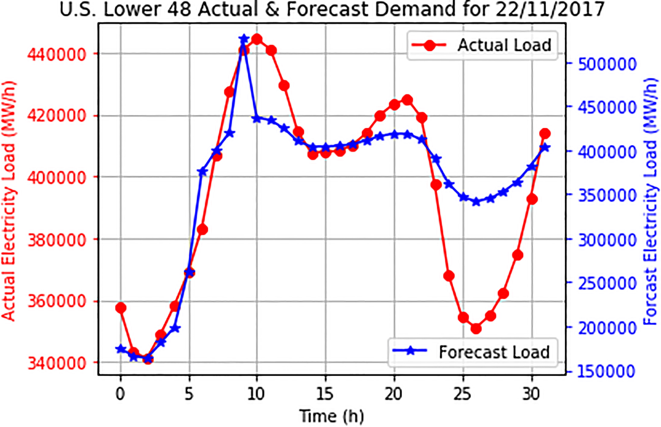

Often, forecasting problems relating to a disparity between electricity demand and forecast were due to weather profile variations in the location where the electricity was being consumed [12]. In addition to helping make predictions, Luis [12, 13] highlights a growing interest in this phenomenon by showing the relationship between weather variables and changes in electricity load consumption: knowing the influence the weather has on user consumption can only result in effective future planning.

Classical models have been used, but have proven to be inefficient in terms of short-term load forecasting in a smart grid (SG) [8]. In statistical modelling techniques, regression and time-series models were a huge success, and, more recently, computationally intelligent techniques such as artificial neural networks (ANNs), support vector machines (SVMs), self-organization maps (SOMs) and fuzzy logic have contributed immensely to STLF implementation. These models are excellent, and have been applied in electricity prediction using weather variables in gathering knowledge for demand planning. However, because of the uncertain nature of electricity consumption, they still require enhanced data engineering with regard to accuracy when used for short-term load forecasting [4]. Cooperative techniques which involve collaboration between more than one model, have proven to be more efficient and accurate [14]. In this regard, a cooperative model based on certain data-engineering principles can dramatically reduce the large forecasting errors inherent in classical techniques [1].

1.1 Research question and outline

This paper considers the effect which each weather variable has on load consumption, by using the near-zero error cooperative PSA-DT model. The authors pose the question: “How can an efficient cooperative model accurately predict future load consumption when multiple weather variables matter for STLF of electricity demands in smart grids for smart homes through intelligent data analysis?”. The model uses a probabilistic method to obtain the initial predictive load consumption with a high level of confidence. Before making a final accurate decision as part of productive planning, a decision tree (DT) technique is integrated with the probabilistic model. Here, the focused cooperative model is described through an intelligent data analysis of electricity load and weather variables. The analysis of weather profiles on load consumption helps to deduce the extent to which each weather parameter affects load consumption, where the goal is to determine its predictive accuracy error, compared to the classical model when used to predict future consumption for different user categories. Greater consideration is given to how each weather profile (temperature, wind speed, dew point, humidity and pressure) affects such predictions. The major contributions this article makes to the field of (IDA), are the following:

•
Deployment of a cooperative PSA-DT model integrating the data-engineering concept of probabilistic scenario analysis and decision tree techniques for intelligent short-term load forecasting of electricity demand in smart homes, when multiple weather variables matter.
•
Detailed experimental evaluations of the PSA-DT, benchmarked with state-of-the-art techniques on intelligent weather load trend analytics, in terms of predictive errors, using publicly available electric load and weather data obtained from Texas in the United States (US) [15] and the wunderground [16] repository.

To the best knowledge of the authors, this research performs better than SVM and Artificial Neural Networks (ANNs) when multiple weather variables are integrated (temperature, pressure, relative humidity, dew point and wind speed), in relation to predictive error reduction for short-term load consumption within a smart grid (SG). The remaining parts of this paper are arranged as follows: Section 2 provides a detailed comparison of the traditional power grid and SG framework, including the electricity value chain. In addition, part of the energy load predictive model used in the SG including predictive processes within the grid – is discussed. In Section 3, the fusion of PSA-DT with weather variables, including the underlying mathematical analyses in the model, are discussed. Section 4 comprises detailed experiments and an evaluation of each weather variable on the classical and the cooperative methods. Finally, concluding remarks and future research foci are shared in Section 5.
2. Preliminaries

2.1 Traditional electricity grid

A traditional electrical power grid is a one-way electrical transmission and distribution system where electricity can only flow in one direction, from the generating station to the consumer [17]. This ancient grid has been in existence for more than a century, and is subjected to several challenges from the distribution point until it reaches its destination (where power is consumed). Such challenges, according to the Department of Energy [18], include 6% distribution and transmission losses in the US and even greater losses in less developed economies, greenhouse gas emission, and, more recently, security issues from energy suppliers, an alarming demand for more electricity, and poor management and control of the electricity distribution grid.

2.2 Electricity value chain

Several processes involved in transmission, substation step down and the distribution chain occur between the generation of electricity at the source, and the point of consumption by customers [18, 19]. Shown in Fig. 2 is a typical electricity power chain delivery framework that indicates the transition from generation to various consumers. Importantly, the substation and primary consumers are mostly medium and large businesses that are financially buoyant enough to own personal transformers, while secondary consumers are mostly residences and small businesses.

Figure 2.

Typical electricity value chain in classical power delivery system.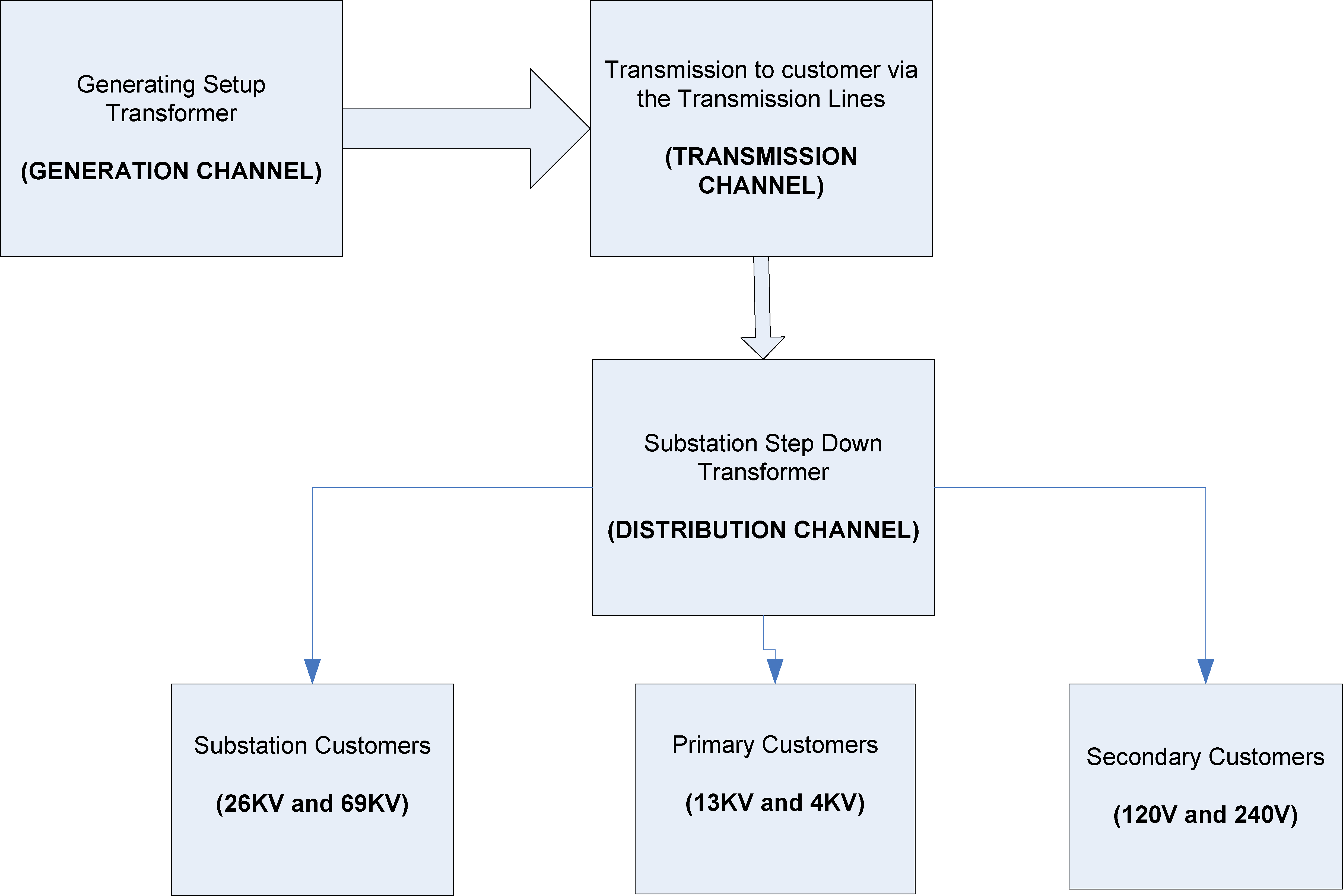

According to the Department of Energy [18], classical power chain delivery faces various challenges, such as losses at each stage ranging from generation to transmission, and also before reaching the final consumers, as shown in Fig. 3.

Figure 3.

Power losses in the grid.

Despite losses at every stage in the electricity value chain, the current state of the grid shows an imbalance between the energy supply and the aged electromechanical (traditional) grid. In addition, an increase in demand, insufficient thermal generation, an inability to integrate with another renewable energy, aging grid infrastructure, several security setbacks, and inconsistent regulatory and legislative environments represent some of the major challenges facing traditional grids. These challenges make such a system inconsistent and unsustainable. However, moving to a sustainable grid requires the invention of a smart grid whose characteristics include increased power transmission and efficiency, the optimization of grid assets, intelligent and end-to-end monitoring, control with a cybersecurity focus, customer engagement and extensive demand response.

2.3 Transition from traditional load distribution to smart grid

In today’s world, information technology has transformed every facet of the economy, including electricity generation, distribution and transmission. A traditional grid is characterized by customers’ non-participation in the power system and their slow responses, a central generation of power supply replete with obstacles and power losses, inefficient operations and assets management, and, above all, inefficient responses to assets handling. The reverse situation obtains in a smart grid, known as the grid of the future, which might be subjected to certain threats (such as a vulnerability increment that makes it prone to cyber-attack, unstandardized technology usage, upfront consumer expenses and infrastructure mismanagement). Table 1shows some of the functional differences between a smart and a traditional grid.

Table 1
Classical differences between traditional and smart grids

Considered factors	Smart grid	Traditional grid
Easy and quick resolution of FLISR (fault location isolation and service restoration)	Yes	No
Real-time and ease of management (transmission, delivery and monitoring) [20, 21]	Yes, remote	No, onsite
Enhances analysis of the collected data	Yes	No
Consumers play a critical role in grid operation, especially in optimization	Yes	No
System design	Digital & microprocessor or	Electromechanical and solid state
	microcontrollers
Communication flow	Global two-way communication	One or local two-way communication
Resilience	Self-healing and automated	Manual restoration
Reliability	Predictive reliability	Estimated reliability

2.4 Smart grid

Information and communication technology (ICT) is one of the most essential components of technology-driven industries in today’s economy, and its usage in renewable energy is no exception. ICT has been integrated with renewable energy – especially the power grid – to make such a grid more intelligent, hence the reference to a smart grid. An SG is one of the most critical infrastructures in a classical power grid, containing several smart objects such as a smart meter, smart devices, sensors, actuators, and, to cap it all off, a communication infrastructure for seamless communication among the various components.

SGs are also referred to as intelligent power grids (IPGs). An IPG forms its chain from the energy generation point through power-transmitting infrastructure and distribution networks to the final electricity consumer (homes, factories, public lighting, smart appliances and electric vehicles, to mention a few). In addition, making such a power grid ‘intelligent’ requires some level of ICT involvement (hardware, software and firmware) to ensure proper control and remote monitoring of the grid, and keep a real-time balance between electricity generation and consumption. Moreover, electricity consumers extensively dictate production from the power grid – knowing their daily consumption helps in developing prior knowledge of their future consumption.

In addition to the description of an SG, it would be nice to have the key drivers that determine the continuous growth of a ‘smart grid world’ and the various benefits derived from such inventions. The key drivers of a smart grid are growing energy demands; energy-independent infrastructure; the necessities linked to reliability and security; economic growth and sustainability; technological advancements; everything necessary to ensure quality power; and safety necessities for all grid workers.

In summary, various benefits such as quick recovery during storms; a reduction in the cost of utilities; effective customer engagement and the efficient breakdown of silos in utility operations (such as system operation and protection) can be derived from an SG, rather than a traditional grid.

Table 1 provides an overview of the actions associated with smart and traditional grids (see [20, 21, 22]).

2.5 Prediction methods for energy load

The energy in a smart grid can be effectively addressed using two major approaches: either artificial intelligence techniques or statistical methods. Some of the reviews reported on in [4, 10, 23, 24, 25], for electric load forecasting, range from time series to regression-based methods (statistics-based techniques), while artificial intelligence methods range from the ANN and fuzzy inference techniques to support vector machine (SVM). Feinberg and Genethliou explain the different methods used for various load predictions [25]. Each forecasting technique has merits and demerits in terms of its ability to accurately forecast future load. Regression techniques are the most widely used statistical techniques for electric load forecasting [26]. Used for modelling the relationship between load consumption and other factors, such as weather and season, they tend to measure the extent of the relationship between the dependent and independent variable [27]. These techniques have found the greatest relevance in offline (non-real-time) forecasting, but are generally unsuited to online forecasting because they require many external variables that are difficult to introduce into an online algorithm [26]. A similar approach to regression is the time series analysis method, which includes linear and dynamic regression. It is also a widely used statistical technique for electric load forecasting [26]. To address the lacuna in the forecasting of both online and offline loads, an exponential smoothing model presents an appealing load forecasting tool [28]. However, it has poor long-range accuracy with regard to weather information, therefore this technique cannot account for weather-related load changes. Another robust statistical technique which is related to machine learning is the Bayesian Network (BN). BN, which is able to handle missing values very well, yields a positive result during queries when compared to a training dataset in the case of machine learning techniques such as ANN or SVM [29]. Being a probabilistic model, it shows the relationship between random electricity and weather variables.

In addition, the use of artificial intelligence techniques has raised hopes for the various challenges facing the use of statistical methods. Using ANN techniques, Hahn et al. [23] found that a number of neural networks performed best with a small mean percentage error (MAPE) of between 2.35 and 2.65%, and a minimized spreading of errors. Adversely, neural networks require significant training for users to understand the model [24]. The widely used ANN method of electric load forecasting is back propagation.

Another powerful artificial intelligence method used for electrical energy prediction is SVM, especially for solving classification and regression issues [27, 30]. The aforementioned authors highlight the efficiency of SVM for the nonlinear mapping of datasets into prominent dimensional features via kernel functions, which perform better than statistical techniques. Several researchers [31, 32] mention that support vector regression, being a variant of SVM, avoids under- and over-fitting training data by minimizing the training error as well as regularization. Nevertheless, one of the biggest limitations of these techniques is the inability to choose a suitable kernel [26]. The difficulties of interpreting the meaning of the numbers derived from this model were seen as a further drawback [8]. Therefore, SVM, if used for predictive modelling, requires a trade-off of predictive power with the difficulty in interpretation [8].

2.6 Predictive data analysis phases

During the research phase, electricity load and weather parameter data were collected, cleaned and analyzed prior to making predictions regarding future load consumption. The analysis processes involved data collection, wrangling, exploring, transforming, modelling, visualization, pattern recognition, and finally an evaluation of the performance of the model, as shown Fig. 4, with a brief annotation in each phase.

Figure 4.

Predictive analysis phases (adapted from [34]).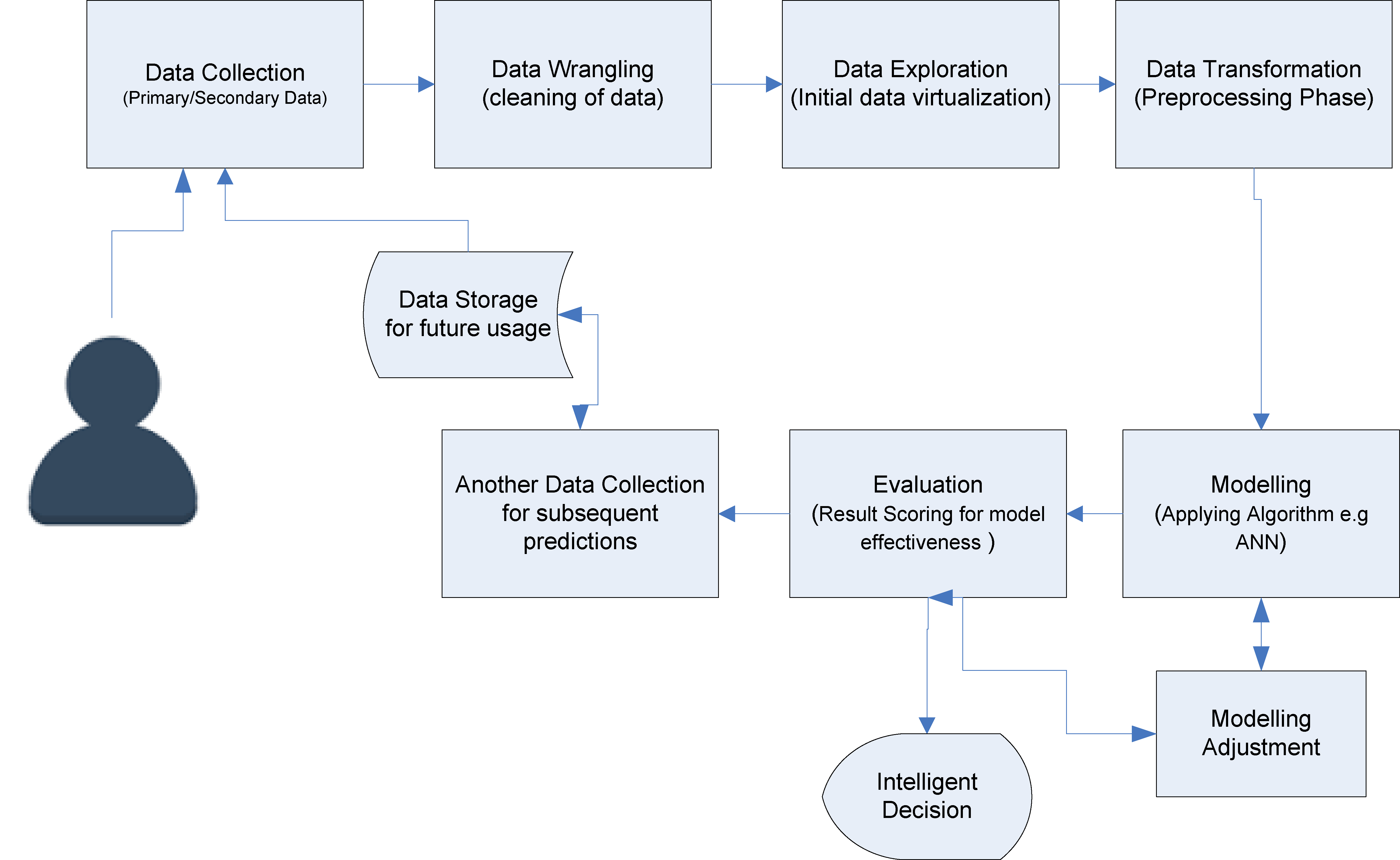

2.7 Theoretical techniques

2.7.1 Probabilistic scenario analysis (PSA)

PSA, being the use of a probabilistic model across various scenarios, foresees and evaluates a variety of possible occurrences of an event in the future [35, 36]. It is often used in the financial world to make extensive projections into the future. Considering the technique and its vast usage in management for future forecasting, several researchers have come up with diverse processes in performing good scenario analysis [37], which can easily be combined with the probability model to generate a sampled expected outcome based on randomly generated events [38].

In the proposed technique, especially during simulation processes, the cumulative probability $f(x)$ of the load consumed is being computed as a non-decreasing function, with probability values between 0 and 1. In this regard, the expected mean in Eq. (1), generated during this random process, will have a certain level of confidence which falls between the confidence interval for the entire load samples usually known as the t-interval, as shown in Eq. (2). Equation (3) shows the deviation from the population mean for the generated values.

$\displaystyle\textit{mean}\left(\mu\right)=E\left(X\right)=\mathop{\int}% \limits_{-\infty}^{\infty}xf\left(x\right)\delta x\text{ where }f\left(x\right% )=P\left({a\leqslant x\leqslant b}\right)$ (1) $\displaystyle t_{\textit{interval}}=x\pm T_{\alpha/2,n-1}\times\frac{\sigma}{% \sqrt{N}}$ (2)

Where $E(X)$ is a point estimate of $\mu$ , $\frac{\sigma}{\sqrt{N}}=$ standard error of the mean and $T_{\alpha/2,n-1}\times\frac{\sigma}{\sqrt{N}}=$ error margin

$\displaystyle SD=\sqrt{\left(\frac{1}{N-1}\sum_{i=1}^{n}(Yi^{\prime}-Y)^{2}% \right)}$ (3)

2.7.2 Decision tree (DT)

A DT uses a tree-like pattern to present various possibilities for its decision route and the result of each route, in order to decide effectively on the path to take, depending on whether it is a classification or a regression problem. It uses entropy or information gain to predetermine its possible split point in the classification problem, while standard deviation from the mean forms the major criterion for a split in the regression problem.

Entropy: This is a measure of disorderliness or impurities in the sample space, and its computation has been formalized by Shannon [38, 39]. Let us assume a random variable $X$ , with values $x_{i}$ and probability ( $x_{i}$ ), has its entropy in Eq. (4).

$\displaystyle H\left(X\right)=-\mathop{\sum}\limits_{i}\Pr\left({x_{i}}\right)% \log 2\Pr\left({x_{i}}\right)$ (4)

3. Cooperative PSA-DT model for short-term load forecasting when weather variables matter

This section mainly focuses on the development overview of a cooperative model for short-term load forecasting in an SG environment, by using the predictive result for effective future demand and operational planning. Greater consideration is given to weather variables on such predictions. In this model, load consumption from various classes of consumers (residential and commercial) and the corresponding weather profiles (temperature, wind speed, dew points, humidity and pressure) were considered. The collected historical load data were cleaned and formatted for effective integration. The PSA-DT cooperatively functions as an engineering between-scenario analysis, with a probabilistic focus. A DT model as described in Section 3.4, and the high-level diagram is shown in Fig. 5.

Figure 5.

Engineering of predictive STLF with weather profile framework.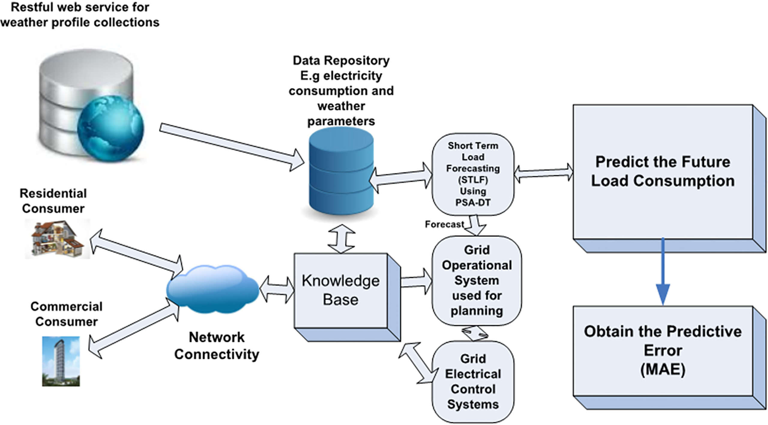

The data-engineering components in Fig. 5 comprise the historical data repository, grid operational planning systems and the PSA-DT framework. Intelligent sensors installed in the SG were used to capture the hourly frequency of the load being consumed by residential and commercial users, and stored this in the repository once it had been filtered by the knowledge-based system. Based on the location where the load was consumed, each weather profile (temperature, wind speed, dew point, humidity and pressure) was fetched through our custom-built Restful web service from wunderground and stored in the data repository (see Fig. 5). These collated data were stored for future predictions and research. The grid operational system comprises control systems and various operational components such as smart electric meters, communication infrastructure and several planning tools, among which is the STLF model for effective load planning. The predictive framework describes the process of achieving our predictive results using PSA-DT and the detail analysis of using both Monte Carlo PSA and a DT for a near-zero short-term load predictive solution.

The concepts of confidence interval (CI) and degree of freedom (DF) were also used in the decision process.

The CI shows the stability of an estimate (E(X)) and its measurements closeness to the initial value in a random experiment. It can be calculated using $\mu\pm E_{m}$ where the mean ( $\mu$ ) and $E_{m}$ is the expected error with standard deviation ( $\sigma$ ) component. The estimate at 90%, 95% or 99% confidence level can be calculated prior to the evaluation of an estimate of a high degree of confidence and with uniform probability of occurrence can be fed into the DT for the final prediction of future load consumption.

The DF computed as sample size (N) – 1 simply refers to the number of independent items of information used for computing an estimate.

3.1 PSA-DT: Monte Carlo probabilistic SA modelling with weather profiles

Using PSA-DT for the future prediction of loads involves an active consideration of the expected loads obtained from the sample loads. This result was arrived at through a Monte Carlo random experiment due to the unpredictability of the future load consumption. A flow process is sued that includes obtaining historical loads and corresponding weather locations, and generating the expected load via a Monte Carlo random experiment, to obtain loads of high confidence value. For the selected sample load, the corresponding expected weather profiles were also obtained for easy synchronization during training on the DT model. This flow can clearly be seen in the model’s pseudo code, as shown in Fig. 7.

However, the relationship between the electricity load consumption and weather parameters is evident in the cumulative mean generated from the random sampling in a Monte Carlo experiment, as shown in Eq. (5).

$\displaystyle E_{\textit{demand}}=\left({\alpha_{0}+\alpha_{1}\gamma_{\textit{% mean}\left[1\right]}^{1}+\alpha_{2}\gamma_{\textit{mean}\left[2\right]}^{2}+% \ldots+\alpha_{t-1}\gamma_{\textit{mean}\left[{t-1}\right]}^{t-1}}\right)/n+% \varepsilon_{\textit{margin}}$ (5) $\displaystyle E_{\textit{demand}}=\varepsilon_{\textit{margin}}+\frac{1}{n}% \mathop{\sum}\limits_{t=0}^{t-1}\alpha_{t}\gamma_{\textit{mean}\left[{t-1}% \right]}^{t-1}$

Where $E_{\textit{demand}}$ is the expected load demand, $\gamma$ is the average summation of load and weather variables at every time $t$ , generated through Monte Carlo simulation, while $\alpha$ depicts the constant factor for each of the experiments and $\varepsilon_{\textit{margin}}$ means the possible error margin generated during the process of simulation. The expected load demand can then be predicted using the PSA-DT model in Fig. 7. The major difference between the pseudo code in Fig. 7 and the referenced PSA-DT model is the addition of weather variables during the process of prediction.

Furthermore, using the DT model for the final prediction of the short-term load requires the expected mean in the list generated from the Monte Carlo experiment to be divided into training and test data. In each feature in the training set, a set average and standard error were calculated; a target variable within the training set with least standard error was selected to enhance the split point of the training set into two sets, namely S1 and S2. These operations were then carried out recursively until the leaf nodes were reached. In addition, the lowest error used in determining the split point shows how close the predicted value can effectively fit the test value with a near-zero error value. The prediction and the MAE for the load consumption were finally computed. Based on the DT framework, the operations described above were broken down for a quick view and a comprehension of similar approaches, using the decision rule in Fig. 6.

Figure 6.

A typical DT structure.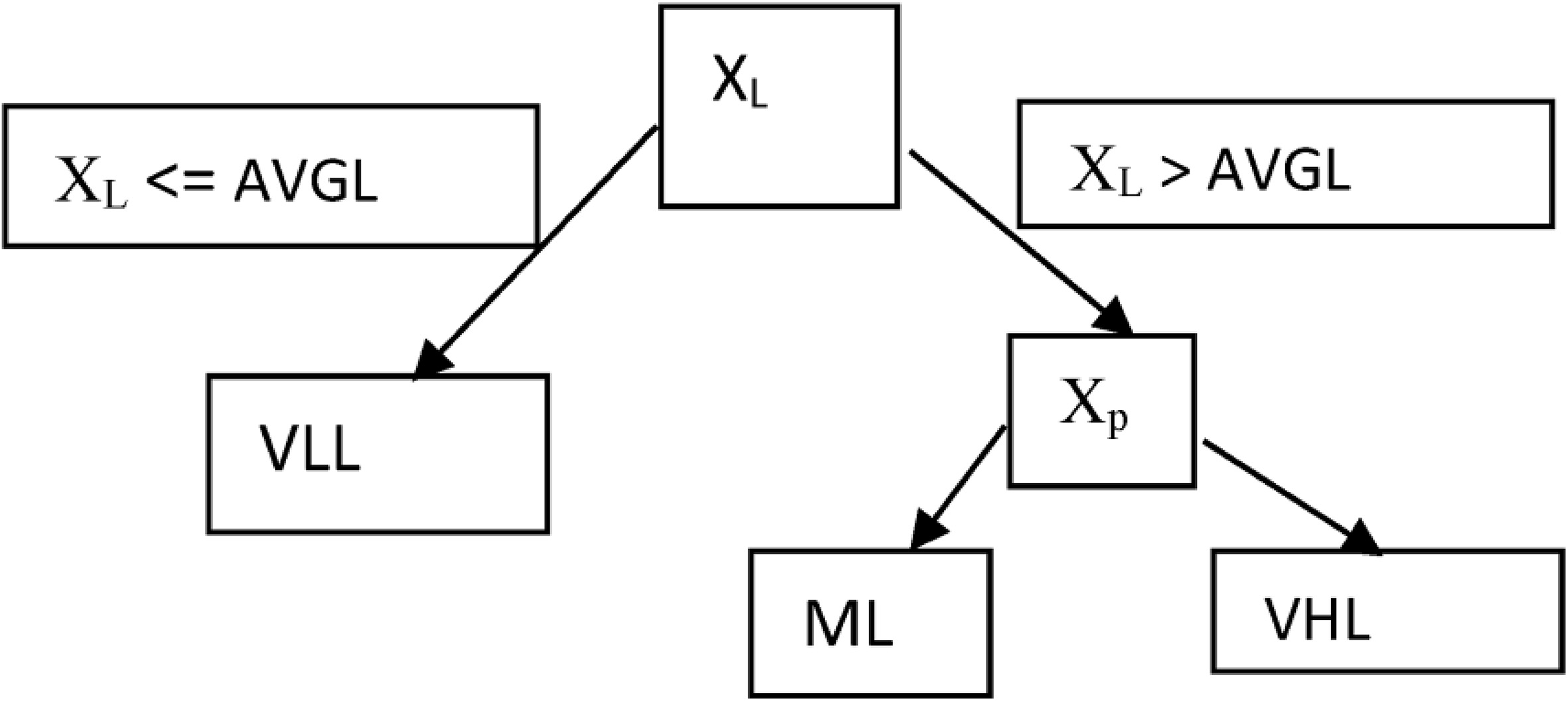

Definition: Consider a DT structure for the load recognition problem described by the following properties: $\text{X}_{\text{L}}$ is the load consumption, $\text{X}_{\text{p}}$ is the absolute weather status, and Y constitutes a set of possible behaviors exhibited by the entities in X, which are {very low load (VLL), moderate load (ML), very high load (VHL)}.

In this case, Fig. 6 shows the model situation where Y depends on X after the average load (AVGL) has been computed.

3.2 PSA-DT: Algorithmic and mathematical analysis

Figure 7 is the pseudo-code used to develop implementation for the PSA-DT model with weather variables. Having read all the electricity load data from the stored repository and fetched the load-corresponding weather parameter through custom Restful web service, the number of simulations for the experiment was inserted. An empty list was generated and the load was finally classified into different load scenarios. The random number of sampled mean was also computed in order to produce the expected mean being stored in an array. The resulting list was used to compute the confidence interval, as revealed in the pseudo-code in Fig. 7.

Figure 7.

PSA-DT with weather profile pseudo-code.

3.3 Evaluation mechanisms

In our experiment, mean absolute error (MAE), being an evaluation metric for predictive modelling performance, was also used to measure the level of closeness of the prediction to the actual outcome. It can be calculated as in Eq. (6).

$\displaystyle\textit{MAE}=\frac{1}{N}\mathop{\sum}\limits_{i=1}^{n}\left|{y_{i% }-x_{i}}\right|$ (6)

where $n$ is the number of observations, and $\left|{y_{i}-x_{i}}\right|$ are the absolute errors between the predicted and actual loads.

3.4 Residential load consumption with temperature weather variable: Numerical scenario

Suppose there is a sample set of very high residential load consumption from an SG, $RL_{vh}$ , which is equal to {3.8809, 3.7225, 3.6137, 3.4286, 3.3893, 3.5024, 3.8319, 3.74693021, 3.74657042, 3.74643688} in kW/h with {6.1, 5.6, 3.9, 2.8, 2.2, 1.1, 0.6, 1.1, 3.9, 6.1} as corresponding temperature at the location of each load consumption. Based on the randomly generated estimated load data from Monte Carlo simulations through randomly sampled residential load from the set $RL_{vh}$ , the following list, $\mu_{vh}=$ {3.74747941, 3.74715633, 3.74683391, 3.74706542, 3.74670404, 3.74693522, 3.74679607, 3.74693021, 3.74657042, 3.74643688} was generated as expected load in the simulated experiment with mean ( $\mu$ ) equals 3.7499 and standard deviation ( $\sigma$ ) equals 0.1224.

The 95% confidence level, sometimes called the margin error ( $E_{m}$ ), can be obtained from the calculation in this section.

Using Eq. (2), N $=$ sample size $=$ 10, $\mu=$ 3.7499 and $\sigma=$ Standard deviation $=$ 0.1224, $\alpha=$ Confidence level $=$ 95% $=$ 0.95. From Section 3, DF $=$ 10 $-$ 1 $=$ 9, $\sigma/\surd n=$ Standard error $=$ 0.1224/ $\surd$ 10 $=$ 0.0387.

Being a component in Eq. (2), $T_{\alpha/2}=$ Confidence coefficient $=T_{\textit{value}}$ (1-confidence level)/2 $=$ (1 $-$ 0.95)/2 $=$ 0.025. We can then extract the result of $T_{\textit{value}}$ (0.025) $=$ 2.262 from T distribution section in [40] and also $E_{m}=$ 2.262 $\times$ 0.0387 $=$ 0.0875. Therefore, the confidence interval at 95% confidence degree $=$ 3.7499 $\pm$ 0.0875: lower limit with 95% confidence interval $=$ 3.7499 $-$ 0.0875 $=$ 3.6624; and upper limit with 95% confidence interval $=$ 3.7499 $+$ 0.0875 $=$ 3.8375.

Despite some low load consumption in $RL_{vh}$ , such as 3.4286 kW/h and 3.3893 kW/h, the expected load for future planning at 95% confidence interval still falls within the range of 3.6624 kW/h to 3.8375 kW/h. In this case, the expected mean $\mu_{vh}$ generated from a Monte Carlo simulation will be between the calculated confidence intervals. Once the statement is valid, the estimated mean has 95% confidence.

Selecting the set of mean loads obtained from the Monte Carlo experiment as $\textit{PSA}_{\textit{result}}=$ {3.7403, 3.74, 3.7401, 3.7398, 3.7397, 3.7398, 3.7406, 3.7408, 3.7416, 3.7415} with corresponding weather equal {6.1, 5.6, 3.9, 2.8, 2.2, 1.1, 0.6, 1.1}, it is appropriate to note that $\textit{PSA}_{\textit{result}}$ falls within the confidence interval and these results were split into training and test sets for DT processing using K-fold CV described in [41].

$DT_{\textit{trainingSet}}=$ {3.7416, 3.7398, 3.7403, 3.7401, 3.7406, 3.7415, 3.7397, 3.7398} the mean of $DT_{\textit{trainingSet}}$ $=$ 3.7404 and the average weather (AVG ${}_{\text{temp}}$ ) $=$ 2.93 $DT_{\textit{testSet}}=$ {3.7408, 3.74}.

Split 1:
The initial split was determined by the weather profile being greater or less than the average weather value. This generated two distinctive sets, S ${}_{1}$ and S ${}_{2}$ , and titled as Set of j ${}^{\text{th}}$ load and Set of i ${}^{\text{th}}$ load respectively (see Fig. 8).

S ${}_{1}=$ {3.7416, 3.7398, 3.7403, 3.7401, 3.7406, 3.7415, 3.7397, 3.7398} $=$ Set of $j^{\text{th}}$ load

S ${}_{2}=$ { } $=$ Set of $i^{\text{th}}$ load

The S ${}_{2}$ becomes the terminated node for the tree, while S ${}_{1}$ follows the process of determining further splitting using the concept of least SD from the mean for all the sets obtained at every tree level.

From Eq. (3), the SD from the mean for $DT_{\textit{trainingSet}}$ is shown in Table 2 for subsequent and different split sessions.

Table 2
Standard deviation for different splitting sessions of the $DT_{\textit{trainingSet}}$

$DT_{\textit{trainingSet}}$ at Split 1 SD at Split 1 $DT_{\textit{trainingSet}}$ at Split 2 SD at Split 2 $DT_{\textit{trainingSet}}$ at Split 3 SD at Split 3

3.7416 0.0012 3.7416 0.0012 3.7416 0.00095

3.7398 0.0006 3.7398 0.0006 3.7415 0.00085

3.7403 0.0001 3.7401 0.0003 3.7397 0.00095

3.7401 0.0003 3.7406 0.0002 3.7398 0.00085

3.7406 0.0002 3.7415 0.0011

3.7415 0.0011 3.7397 0.0007

3.7397 0.0007 3.7398 0.0006

3.7398 0.0006

Figure 8.
Initial decision for weather split.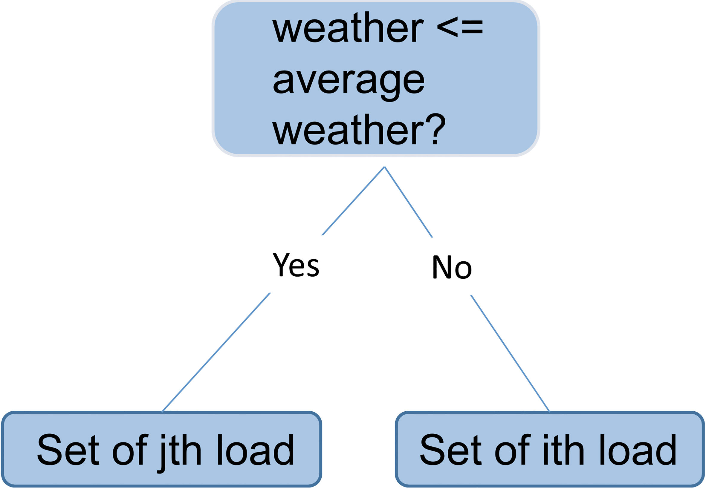

Split 1:
The DT was split where the SD is at minimum value, which is at the point where the load value is 3.7403 kW/h. This is S ${}_{1}$ , while the remaining members in the $DT_{\textit{trainingSet}}$ will form set S ${}_{2}$ , as described in Section 3.3. The S ${}_{1}$ becomes the leaf node while S ${}_{2}$ will go through the recursive process of extracting the member set, with minimal SE carried out in Split 2, as shown in Table 2.
Split 2:
During this split process, the SD of the remaining dataset in Table 2 will be recalculated to obtain the lowest SD value. The load value 3.7406 kW/h with SD 0.0002, being the minimum value among others, is selected as the decision node for further splitting. When the split result is more than one, an average of such result is computed for the leaf node, e.g. (3.7398 $+$ 3.7401 $+$ 3.7406)/3 $=$ 3.7401 kW/h.
Split 3:
At this juncture, the corresponding dataset was used to calculate the SD in order to obtain its lowest SD value. Load values 3.7415 and 3.7398 have the same SD value (0.00085), but the average of the two loads has an approximate value of 3.7407 kW/h, which will form the decision point to aid the final decision. The final leaf nodes in Fig. 9 form the model checked against $DT_{\textit{testSet}}$ for effective testing of the model. $DT_{\textit{testSet}}$ is a new dataset that has never been used during the DT training process and this was used against the training model to obtain an MAE that indicates the model’s predictive performance.

Figure 9.
Generated DT for residential load.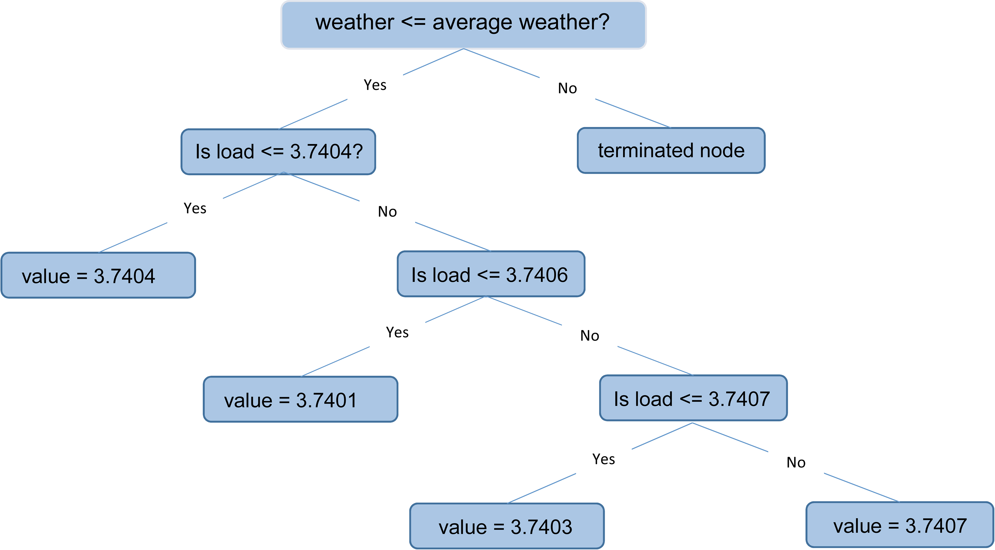

By preference, the last unique leaf nodes are {3.7407, 3.7403}. Therefore, from Eq. (6),

$\displaystyle\text{MAE}=\frac{\left|{3.7407-3.7403}\right|+\left|{3.7404-3.740% 1}\right|}{2}=\frac{0.0004+0.0003}{2}=0.00035$

In brief, the result of the predictive error (MAE) is a near-zero value for the few datasets considered in this mathematical analysis, and compared with the result of the predictive error produced in experiment 2 (see Figs 12b and 13(ii)), it is clear that using the cooperative model PSA-DT produces a near-zero predictive error for residential load consumption. Clearly, most of the error points in the figure revolve around near-zero value.
3.5 Weather data analysis on residential load consumption

$DT_{\textit{trainingSet}}$ at Split 1	SD at Split 1	$DT_{\textit{trainingSet}}$ at Split 2	SD at Split 2	$DT_{\textit{trainingSet}}$ at Split 3	SD at Split 3
3.7416	0.0012	3.7416	0.0012	3.7416	0.00095
3.7398	0.0006	3.7398	0.0006	3.7415	0.00085
3.7403	0.0001	3.7401	0.0003	3.7397	0.00095
3.7401	0.0003	3.7406	0.0002	3.7398	0.00085
3.7406	0.0002	3.7415	0.0011
3.7415	0.0011	3.7397	0.0007
3.7397	0.0007	3.7398	0.0006
3.7398	0.0006

Various weather parameters are critical factors in effective load consumption, and it is necessary to visualize them individually with respect to their corresponding residential load consumption at different time intervals, to determine the relationships in the variables prior to a prediction of future load. Such data visualization aid in expanding the knowledge base on how a weather parameter affects load consumption, offering an instant overview (to be used by the power demand planners for decision making about any location). Shown in Fig. 10a–e are several analytical trend plots for the residential load consumption, with the respective weather variables obtained from the location where the load was consumed.

Figure 10.

Trend analytics with residential data.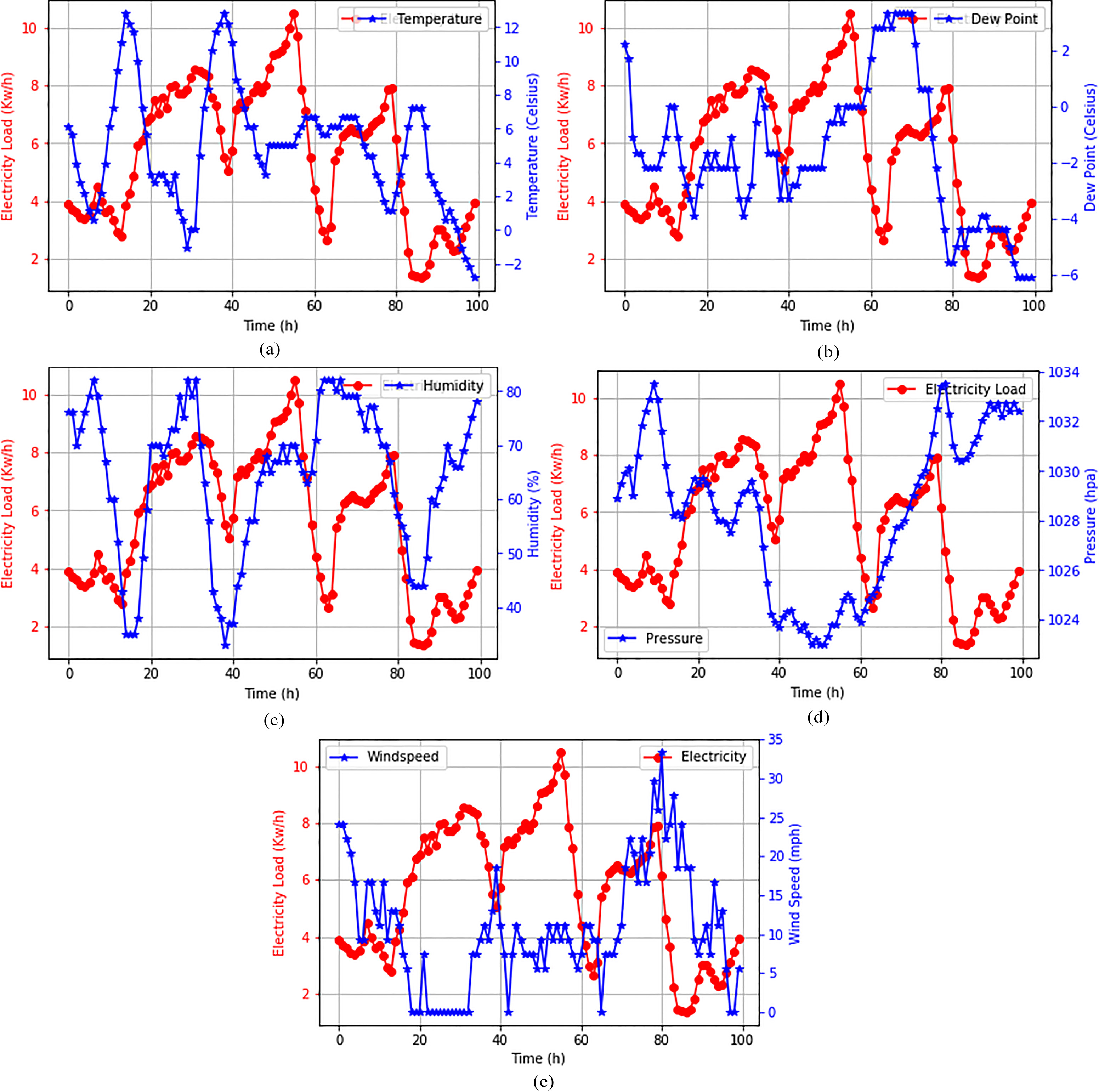

Electricity load consumption behaves in a different way for each weather parameter. By super-positioning the electricity load and weather profiles, it is obvious that there is a direct and an inverse relationship between the two variables at every point in time. One can then deduce generally, from Fig. 10c, that weather variables have some level of direct relationship with load consumption at time 15–42 h, and an inverse relationship between 40 and 60 h in Fig. 10d, 20–60 h in Fig. 10e and 15–80 h in Fig. 10a. These variations in the direct and inverse relationships between the electricity load and each of the weather profiles resulted in uncertain behavior during electricity prediction. This effect simply tells us that there are other factors affecting load consumption, apart from the weather variables, but in this article the major aim is to evaluate the extent to which weather variables can help to reduce predictive errors when forecasting future load consumption.

3.6 Weather data analysis on commercial load consumption

In this section, we visualize commercial load consumption in relation to the various weather parameters, to determine the effect the variables have on one another, as shown in Fig. 11a–e.

Figure 11.

Trend analytics with commercial data.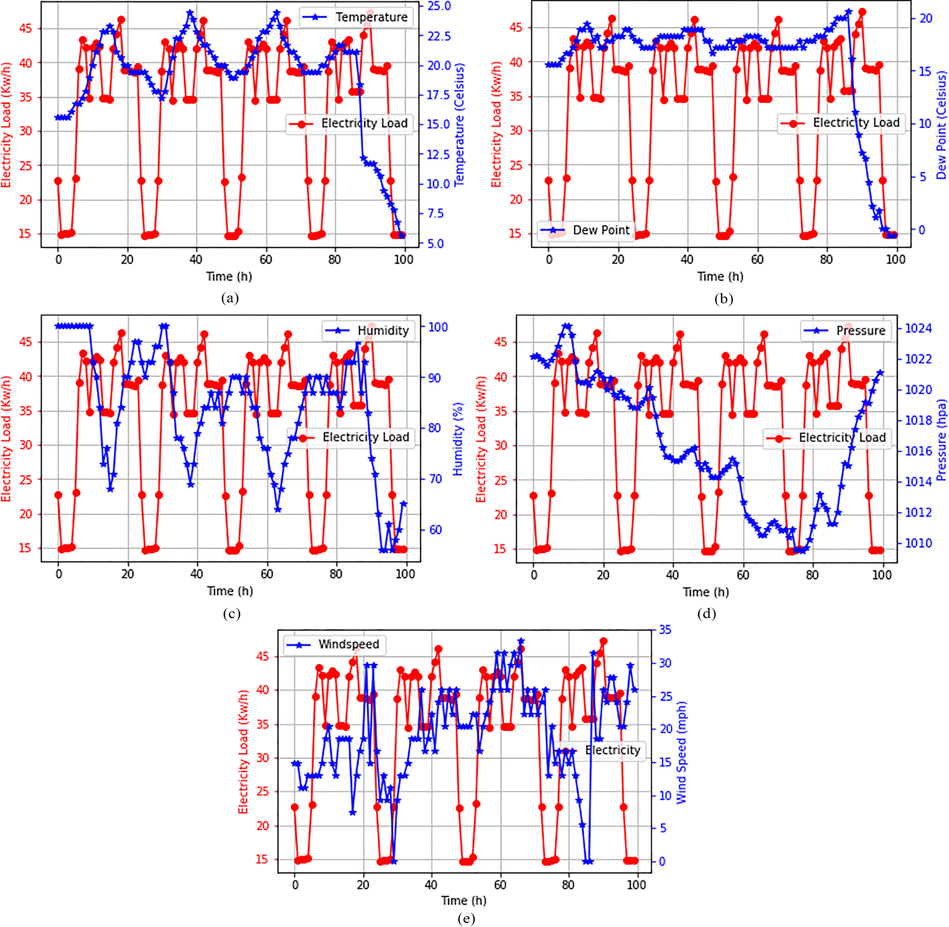

Looking at the pattern in Fig. 11a–e, we can deduce that load consumption reduces at a particular time of the day (especially around 2025 h, 45–50 h, 70–75 h) for all weather variables. Most likely this is the off-peak business period, when load consumers have closed and office equipment has been powered off. The weather variables drawn over the load trends show the behavior of the load with respect to weather factors. Generally, the behavioral patterns of the weather parameters were mostly inversely proportional to the load consumption, with a few exceptions such as 75 h for pressure and 30 h for wind speed, where load and weather were directly proportional.

Having considered the trend analytics from each of the load consumptions in Sections 3.7 and 3.8, it is clear that there is no linear relationship between the load and the weather variables. In addition, the relationship might be directly proportional, and a few hours later it becomes an inverse relationship. This shows how uncertain an electricity load can be. In this regard, PSA-DT being a probabilistic model [42] will be of great value in addressing the uncertainty relationship.

Figure 12.

Snapshot of load consumption and weather variables in smart space by different classes of consumers: (a) Residential data; and (b) Commercial data.

4. Evaluation of predictive data analytics of PSA-DT for short-term load forecasting when multiple weather variables matter for smart homes

4.1 Experimental setup for intelligent data analysis with weather profile

As described earlier, short-term load forecasting corresponds to predictions ranging from one minute to one week ahead. In this research, data collected include residential and commercial loads. The residential and commercial loads were from a location in Texas, obtained as secondary data from open energy information (OpenEI), an open-source energy platform that manages all energy data submitted by industrial experts and enthusiasts [15]. For the reliability/quality of the dataset, OpenEI rendered assistance to various international organizations and diverse partners/sponsors (e.g. ECOWAS Clean Energy Gateway, International Clean Energy Analysis) that assist in enhancing the data and content on this platform. The brief overview of the data layout, shown in Fig. 12, is a snapshot of the various hourly electricity data meant for different classes of electricity consumers and the corresponding weather variables obtained from wunderground [16]. Each electricity consumer and its corresponding weather status at the location of such consumption serves as an entry point to the PSA-DT model, as shown by the processes described in Section 3.3. These hourly time series were used because of difficulties in obtaining a one-minute or 15-minute open-source dataset. The few minutes dataset are usually proprietary. The loads were then stored in the data repository after being processed via the knowledge-based system, with the weather dataset based on the load consumption geolocation. During electricity forecast planning by the grid owners, stored historical records in this repository were fetched by the model to make its prediction.

The major raw input data fed into the designed model were the time series load data and the weather variables for different categories of data collected. The predictive problem was approached by systematically following the PSA-DT pseudo-code in Fig. 7. During implementation, several libraries and types of software, in addition to PANDAS for data analysis, were used [43]. These are matplotlib for data visualization, sklearn package, and a repository of diverse machine learning algorithms where the DT model and other algorithms were obtained for the experiments [41]. In addition, scipy [44] was used for both descriptive and inferential statistics such as mean, variance and standard deviation. Using the random sample experiment, a high confidence-level estimated mean was generated prior to final decision-making via the use of a DT model. This forms the basis of the model explained in this article.

4.2 Experiment 1: Intelligent electricity load forecasting with classical models on residential load consumption with weather variables

In Figs 13a–e and 14a–e, the residential load consumption in kW/h (shown on the $y$ -axis) and the hourly consumption time (shown on the $x$ -axis) were used during the various experimental setups. The load was predicted in parallel with the actual load using the forecasting line until the 50th hour, as shown in the figures in these sections. The 51st and 60th hour are the ten-step forecasting horizons that depict the future predictions for each classical model, based on the residential data in Fig. 13a. The aim is to verify predictive abilities in terms of a reduced MAE for each weather variable used with the load consumption during classical model prediction. Each experiment exhibited slight differences in terms of predictive error, as shown in Figs 13a–e(ii) and 14a–e(ii), for temperature, wind speed, dew point, humidity and pressure. Based on the behaviour of the five experiments, the following reasoning analysis should guide the actions of future electricity consumption planners in their decision processes.

Figure 13.

SVM for residential electricity load consumption with (a) Temperature; (b) Wind speed; (c) Dew point; (d) Humidity and (e) Pressure.

Figure 14.

ANN for residential electricity load consumption with (a) Temperature; (b) Wind speed; (c) Dew point; (d) Humidity and (e) Pressure.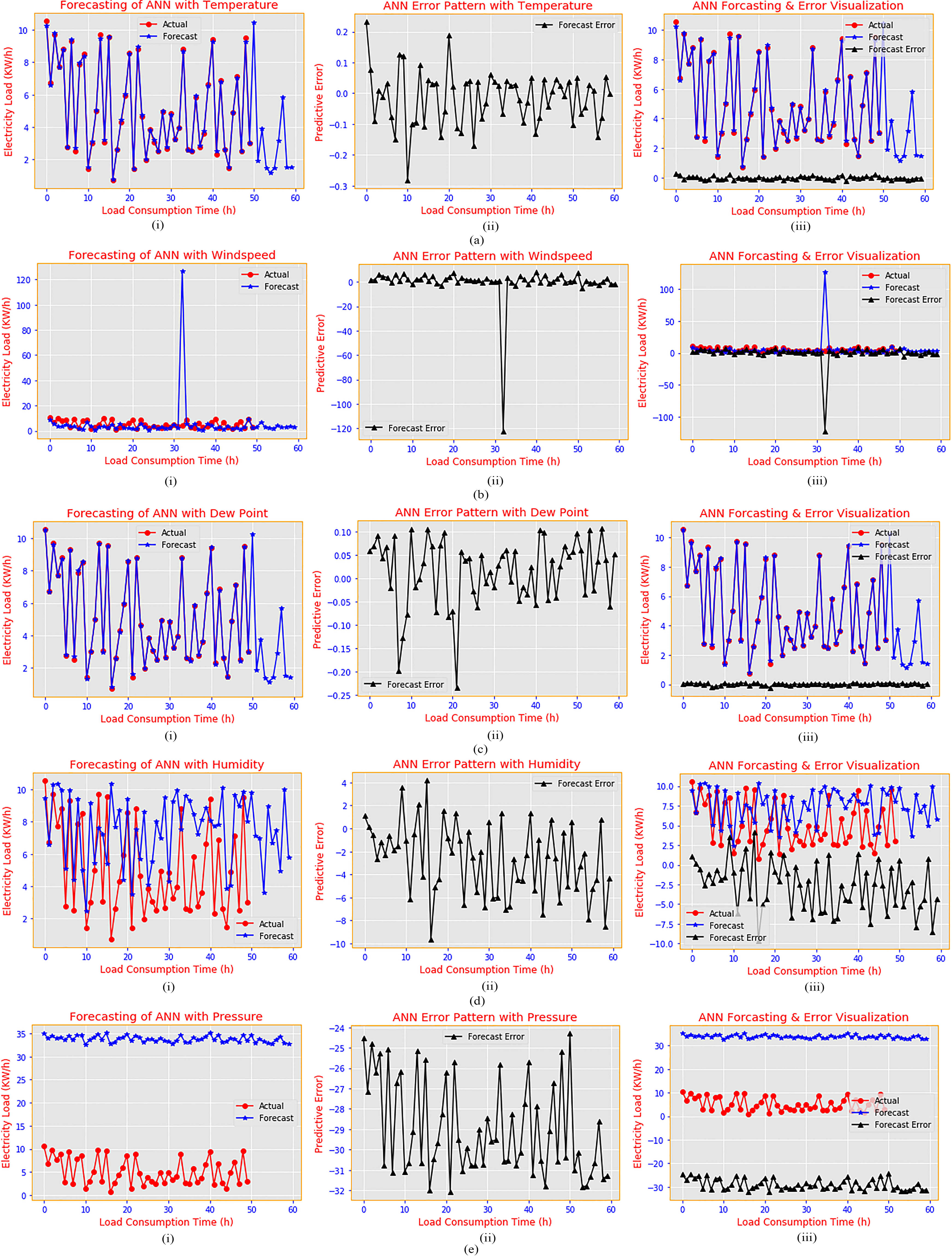

Decision-making: The sampled qualitative analysis between the 51st and 60th hour of this experiment gave a corresponding answer to some of the questions asked.

(Question) Q1: What is happening to the predictive behavior and why is it happening?

(Answer) A1: For SVM in Fig. 13a–e(ii), the predictive errors with temperature and pressure are minimal, with peak values ranging between $-$ 1.8 kW/h and 3.0 kW/h; followed by the predictive error of dew point which is slightly lower than the result obtained from temperature and pressure with error values ranging from $-$ 1.2 kW/h and 2.6 kW/h. The predictive error values for wind speed and humidity are higher than temperature and pressure error, with a value between $-$ 2.8 kW/h and 3.9 kW/h.

For ANN in Fig. 14a–e(ii), the predictive error with dew point is reduced, with peak values ranging between $-$ 0.25 kW/h and 1.20 kW/h; followed by the predictive error of temperature which is slightly higher with an error value of $-$ 0.3 kW/h and 0.23 kW/h. Both temperature and wind speed had an outlier error at 10 h and 31 h respectively. The predictive error results obtained from dew point and humidity ranged from $-$ 0.25 kW/h to 0.1 kW/h and $-$ 10.0 kW/h to 4 kW/h respectively. In the same figure, it shows clearly that wind speed has many data points, with huge predictive errors ranging from 1 kW/h to 19 kW/h, with the exception of the outlier data point at 31 h.

Although the ANN could predict slightly better in terms of low predictive errors compared to the SVM classical model for temperature and dew point (but vice versa with wind speed, humidity and pressure where SVM predictive errors results are lower than ANN counterpart), their predictive performance can still be improved with the PSA-DT model. In addition, the ANN forecasting result in Fig. 14b(i) could not fit the actual load for different load consumption periods with humidity, and this inability is more obvious with wind speed and pressure. This irregularity was because large amounts of data were needed to train the ANN model for effective predictions. Also, the drawbacks of inaccurate predictions and proper fitness of the forecasted load with the actual load for each weather variable also exist with SVM, but such ineffectiveness in predictive performance could be abated with the PSA-DT model.

Looking at Figs 13a–e(i) and 14a–e(i), which are meant for SVM and ANN respectively, weather parameters seem to affect predictive accuracy, especially given the different variations in the predictive error of each weather profile. Also, the forecasting lines cannot accurately ‘fit’ their corresponding actual load lines. Overall, there was an under-estimation.

Q2: What can be done about it and what will happen next?

A2: The forecasting error can be improved by deploying an effective cooperative model to track the inherent uncertainties for the predictive analysis with weather profile. The ANN model tends to predict well in terms of low predictive error for temperature and dew point (see Fig. 14a(ii) and c(ii)), with a predictive error value of $-$ 0.3 kW/h to 0.23 kW/h and $-$ 0.25 kW/h to 1.20 kW/h respectively, when compared to the corresponding predictive error result of the SVM model with weather profile (see Fig. 13).

One can also deduce that the predictive result rises and drops with respect to an increase and decrease in actual load consumption, respectively. To address the results of high predictive errors produced by the classical models, the use of an uncertainty model could be of great value for more reliable electricity load predictions and near-zero predictive errors.

However, note the fluctuating nature of the predictive error over time; due to the unpredictable nature of the load consumption feature and its corresponding weather profiles, this implies that there will be a great need for a probabilistic model (such as the PSA-DT) that can better handle uncertain conditions.

4.3 Experiment 2: Intelligent electricity load forecasting with PSA-DT on commercial consumers with weather variables

The objective of this test and the results obtained, as shown in Fig. 15a–e, is to affirm the effectiveness of the predictive ability of the PSA-DT in terms of the low predictive error computed using Eq. (6) and comparing the PSA-DT predictive error with the classical model error within the context of each weather profile.

Figure 15.

PSA-DT for commercial electricity load consumption in smart homes with (a) Temperature; (b) Wind speed; (c) Dew point; (d) Humidity and (e) Pressure.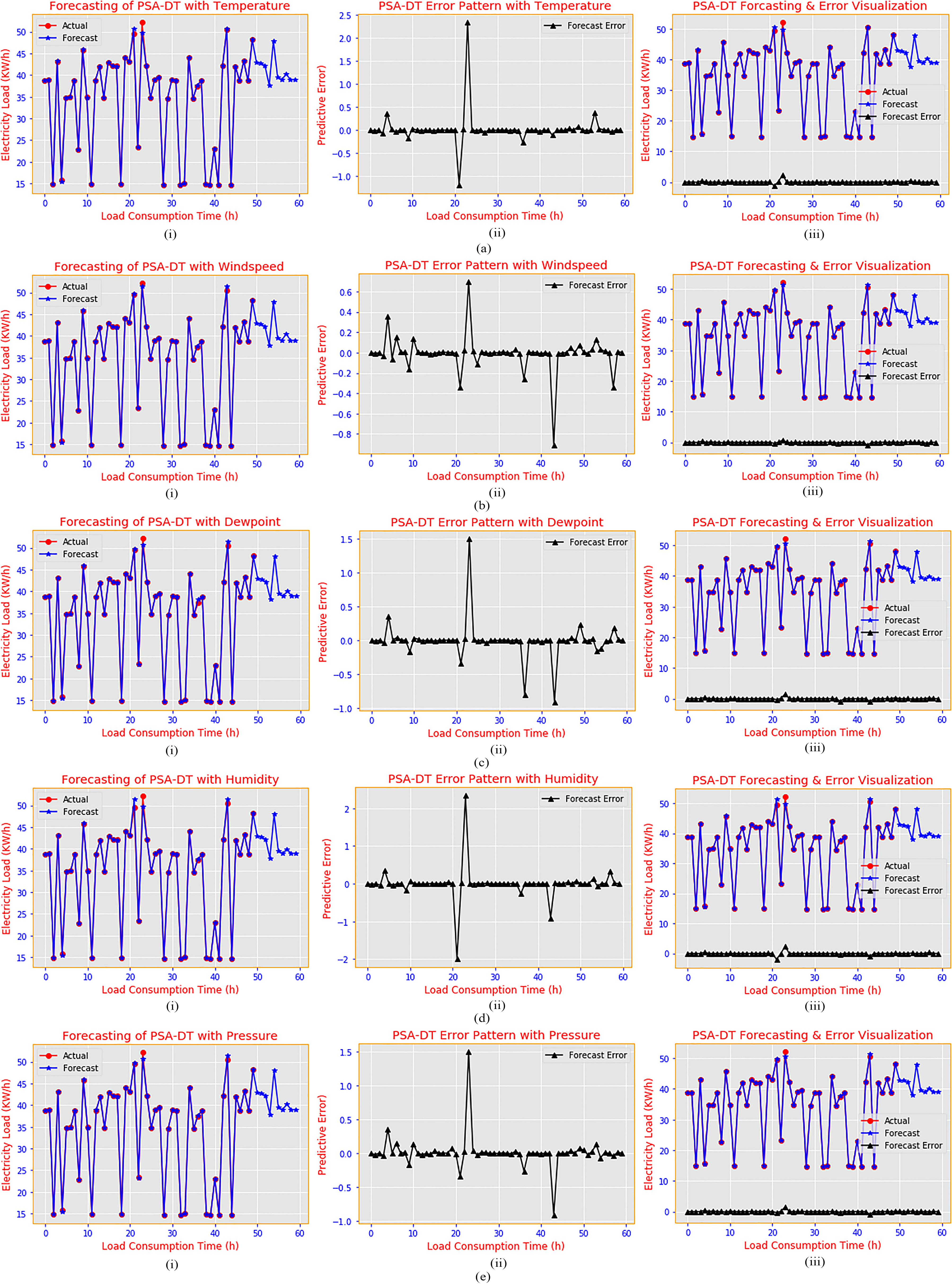

Decision-making: Sampled qualitative analysis between load consumption Hour 0 and Hour 50 and beyond.

Q1: What happens to the predictive behavior and why?

A1: The predictive error for each experiment in Fig. 15a(ii)–e(ii) has its error values for the majority of the load consumption time, with each weather variable close to zero (with the exception of a few outliers at 21 h for temperature; 22 h and 42 h for wind speed effect; 22 h, 36 h and 43 h for dew point; 22 h and 42 h for humidity; and pressure at 22 h and 42 h). This near-zero performance was aided by the probabilistic predictive ability of the PSA-DT, coupled with the weather effect. Since the errors generated by the PSA-DT with each weather parameter are extremely small, compared to the value generated by the classical model shown in Figs 13a–e(ii) and 14a–e(ii), the forecasting result generated by the PSA-DT model tends towards higher accuracy than the result obtained from the classical model for all classes of users being considered.

This predictive error, revolving around the zero points on the axis, occurred because of the meaningful weather parameters, with the cooperative nature of the PSA-DT model formed by combining the merits of both the PSA and the DT model described in Section 3. Due to the uncertain nature of electricity load consumption, the expected mean load with a high confidence value was obtained via the Monte Carlo experiment, before passing the result into a DT for effective learning and predictions.

Q2: What can be done about it and what will happen next?

A2: To maintain the efficiency of the cooperative model with weather profiles, data used for such predictions can be obtained with a low time interval (less than hourly). In addition, acquiring more datasets to train the PSA-DT model could improve the predictive error. Considering weather variables during predictive analytical processes within an SG has huge potential to yield an effective forecasting result with high confidence of low predictive error. This experiment shows the different forecasting abilities and the forecasting error of the cooperative PSA-DT model when used with weather parameters, and for commercial users of electricity load.

In this section, the results of Fig. 15a–e(i) depict how well the forecast load fit the actual commercial load with a near-zero error. The figures exhibited absolute average predictive error values of 0.0057685, 0.026702, 0.0036875, 0.007436 and 0.0031815 for electricity load with temperature, wind speed, dew point, humidity and pressure respectively, which can be seen as a near-zero error value. Moreover, these possibilities occurred as a result of effective PSA-DT model usage, with weather parameters being considered during the predictive analytics.

The researchers deduced from Fig. 15b(ii) that the result of the cooperative predictive model induced with weather profiles produces a predictive error close to zero, with the majority of the absolute value ranging between 0.00 and 0.01, and the peak error found at 20 h and 22 h for all the weather profiles, 36 h for dew point, and 42 h for dew points and humidity and pressure. The peak error must have been caused by other electricity load influencers, which can be considered in future research. This reduction aids the model’s predictive abilities for economic sustainability. The predictive error remains within the range value, which is lower than the predictive errors of the classical models when used by the same load user category as shown in Table 3.

4.4 Experiment 3: Intelligent electricity load forecasting with PSA-DT on residential consumers with weather variables

In this section, the objective of this test and the results obtained, as shown in Fig. 16a–e, affirm the effectiveness of the predictive ability of the PSA-DT in terms of the low predictive errors computed using Eq. (6), and comparing the PSA-DT predictive error and the classical model error within the context of each weather profile for residential load consumers.

Figure 16.

PSA-DT for residential electricity load consumption in smart homes with (a) Temperature; (b) Wind speed; (c) Dew point; (d) Humidity and (e) Pressure.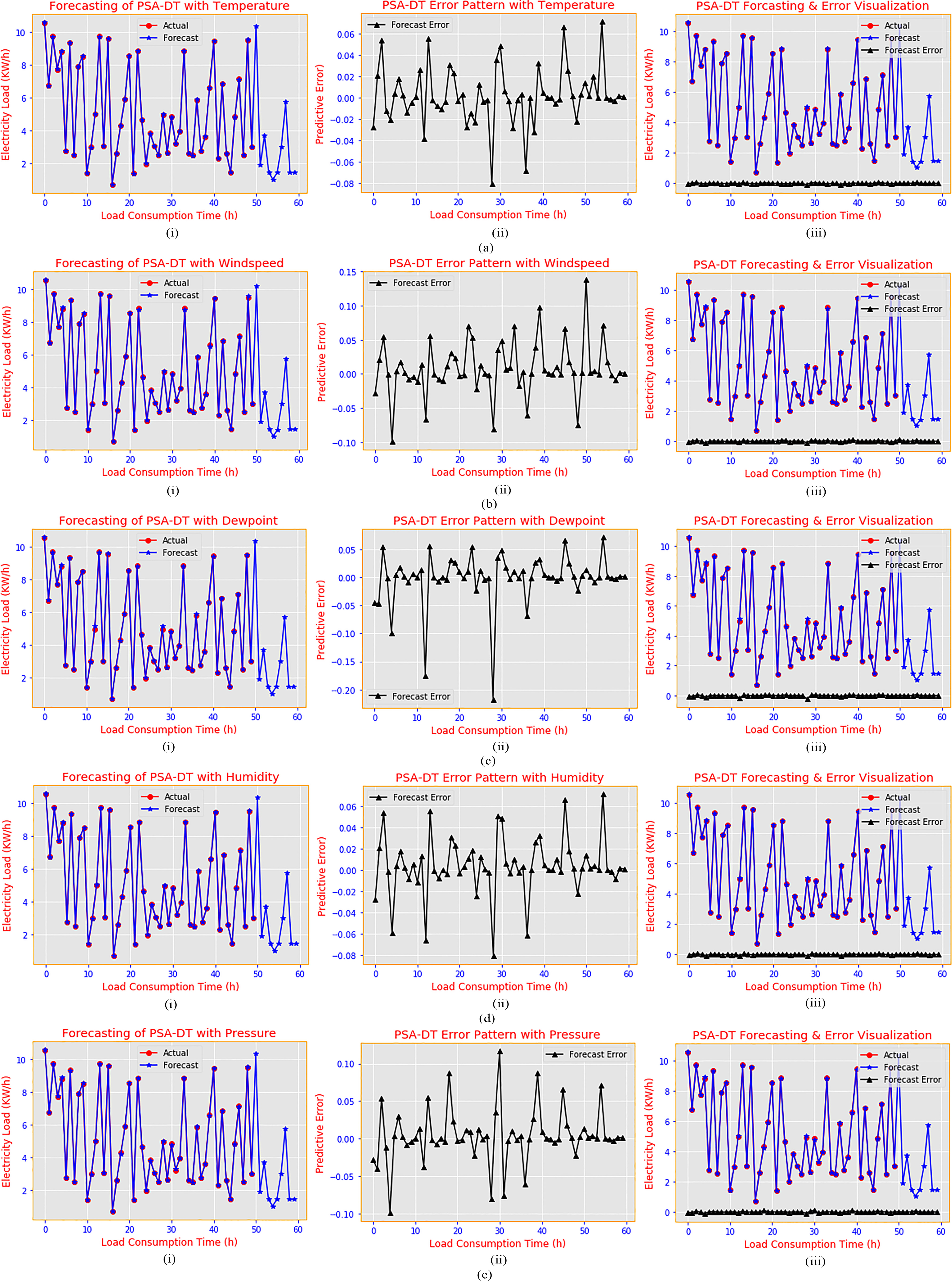

Decision-making: Sampled qualitative analysis between load consumption Hour 0 to Hour 50 and beyond.

Q1: What is happening to the predictive behavior and why is it happening?

A1: The predictive error for each of the experiments in Fig. 16a(ii)–e(ii) has its error values for each weather parameter as follows: temperature ranges between $-$ 0.08 and $-$ 0.07; wind speed ranges between $-$ 0.1 and 0.14; $-$ 0.2 and 0.055 was the error value of dew point; humidity also ranges between $-$ 0.08 and 0.07 and, finally, pressure profile produces an error value of $-$ 0.1 to 0.13. This near-zero performance was aided by the probabilistic predictive ability of the PSA-DT, coupled with the weather effect. Since the errors generated by the PSA-DT with each weather parameter are extremely small compared to the value generated by the classical model shown in Figs 13a–e(ii) and 14a–e(ii), the forecasting results generated by the PSA-DT model tend towards higher accuracy than the result obtained from the classical model, for all classes of users being considered.

This predictive error revolving around the zero points on the axis occurred because of the meaningful weather variables, with the cooperative nature of the PSA-DT model formed by combining the merits of both the PSA and the DT model described in Section 3. Due to the uncertain nature of electricity load consumption, the expected mean load with high confidence value was obtained via the Monte Carlo experiment, before passing the result into a DT for effective learning and predictions.

Q2: What can be done about it and what will happen next?

A2: To maintain the efficiency of the cooperative model with weather factors, data used for such predictions can be obtained with a low time interval (less than hourly). In addition, acquiring more data for the effective learning of the model and for better representation of the future data point in the training data, can improve the predictive error. Furthermore, greater consideration can be given to the price of electricity being supplied to various residents across different locations.

Considering a weather factor during predictive analytical processes within an SG has huge potential to yield an effective forecasting result with high confidence of low predictive error. This experiment shows the different forecasting abilities and errors of the cooperative PSA-DT model when used with weather parameters and for residential load consumption.

In this section, the result shown in Fig. 16a(i) depicts how well the forecast load fit the actual residential load with near-zero error (see Fig. 16a(ii)). For all the weather variables, the majority of the predictive error points revolve around $-$ 0.02 to 0.03, and a periodic peak error value was obtained at 28 h for all the weather profiles. According to Fig. 16a–e(ii), the predictive errors are still lower than the error results of the classical model used for residential load consumption. Moreover, these possibilities occurred as a result of effective PSA-DT model usage, with low standard deviation from the mean load in residential electricity load consumption.

The researchers deduced from Fig. 16a–e(ii) that the results of the cooperative predictive model induced with weather profiles to produce predictive errors close to zero, with most of the absolute value ranges between 0.02 and the peak error found at 28 h for all the weather profiles; 50 h for wind speed; and 3 h, 5 h, 12 h, 36 h, 42 h and 53 h for humidity. This error reduction aids the model’s predictive abilities, and improves its economic sustainability. The predictive error remains within the range value, which is lower than the predictive error of the classical model when used by the same load user category (see Table 3).

Generally, the predictive results in Figs 15a–e and 16a–e were extrapolated after the 50th load data, in order to predict the next few hours between 51 h and 60 h for each experiment. The corresponding reduced near-zero predictive errors in Figs 15a–e(ii) and 16a–e(ii) show how well the cooperative PSA-DT model with weather variables can predict, using interpolated results ranging from 0 to 50th load data value and after the 50th load data value.

From the visualization result, the forecast load line almost ‘maps’ the actual load line with a near-zero forecasting error in the error pattern figures. In addition, ranging from the temperature to the pressure for both residential and commercial load, the analytical plots in experiments 2 and 3 denote that different weather profiles have different load consumption patterns, and the cooperative PSA-DT with weather profiles can predict consumption to a high degree of predictive accuracy, with reduced forecasting errors. Notably, the level of error also varies among the load categories considered, owing to the load consumption behavior of consumers at different points in time, for different locations.

4.5 Intelligent data analytics of PSA-DT on residential and commercial load consumption with weather parameters

Another interesting observation was the cooperative model with all the weather parameters. Considering temperature, wind speed, dew point, humidity and pressure considering the residential and commercial load consumption during the predictive process gave a more pleasing result of near-zero predictive error. The actual load consumption with the predicted load up to the 50th hour and until the 60th hour for future prediction can be seen in Fig. 17a–b. In the residential load category, it is clear from the residential load consumption that most of the predictive error falls between $-$ 0.1 and $-$ 0.05, and within zero range for commercial electricity load consumption. However, the laudable abilities of the PSA-DT used with weather variables made this happen.

Figure 17.

(a) Residential electricity load consumption prediction with all the weather parameters; and (b) commercial electricity load consumption prediction with all the weather parameters.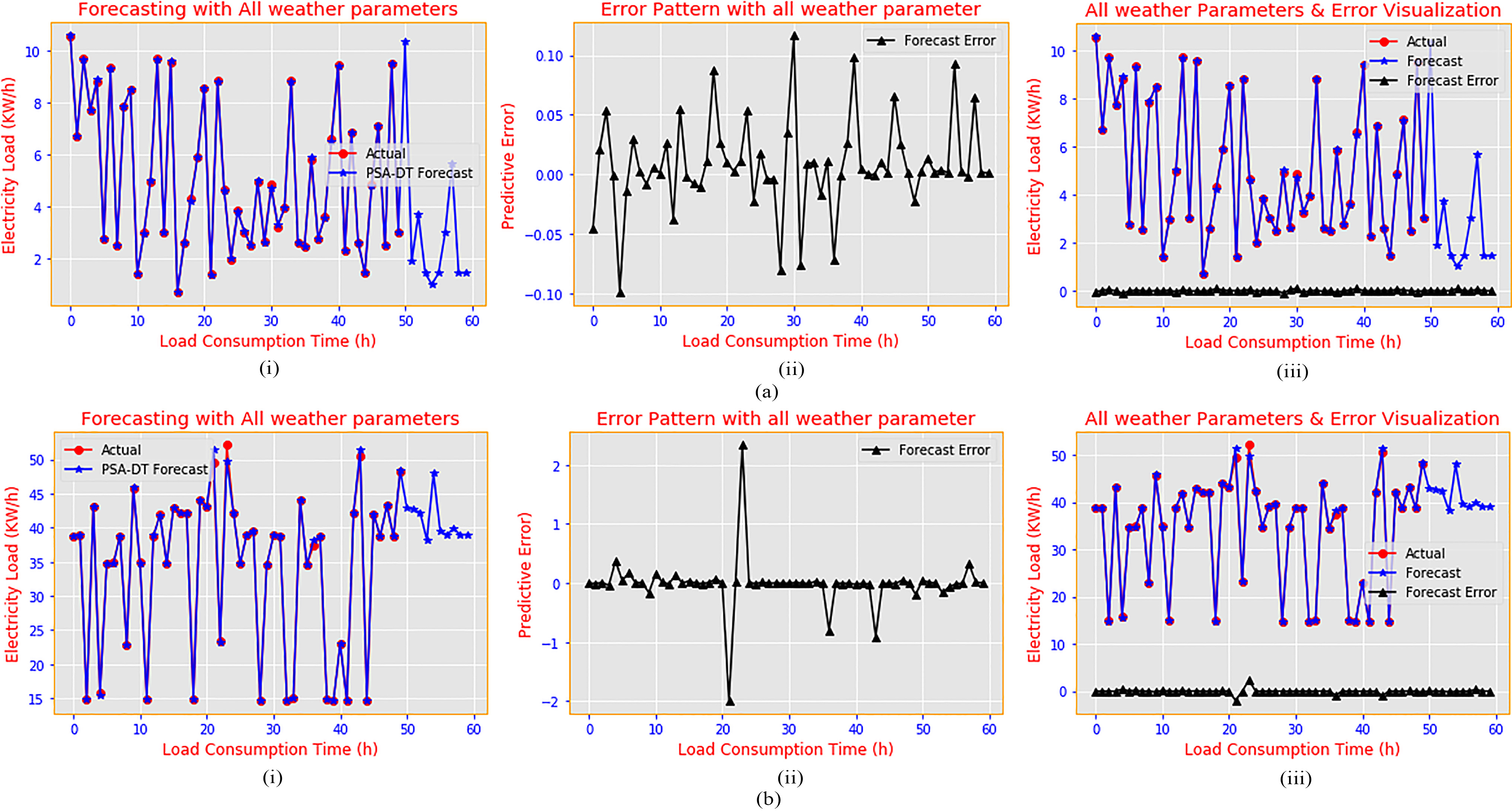

4.6 Intelligent data analytics of electricity load forecasting with PSA-DT and classical models

Finally, a more captivating observation was the cooperative model fitting the actual load consumption compared to other state-of-the-art models at load times up to the 50th hour and until the 60th hour for future prediction (see Fig. 18a and b). In the residential load category, in residential load consumption the “overlap” of the actual load and the PSA-DT forecasting load in Fig. 18a was evident. In Fig. 18b, however, the PSA-DT could fit well into this category, but this was not the case with classical models. The absolute fit of the actual load and the predicted load for the classical model, for both residential and commercial datasets with all weather profiles, could not be extablished due to their performance when compared with the PSA-DT.

Figure 18.

(a) Residential electricity load consumption and (b) commercial electricity load consumption.

This research made differential analysis in terms of forecasting abilities of the PSA-DT when used with weather variables by justifying its performance in reducing forecasting error levels to near-zero, compared to the classical model. The experimental results in Table 3a–b show the various predictive error results of the PSA-DT with each of the weather parameters for different hourly load data, training and test sizes, and each of the classical models. In each table, and for each of the SG user categories including the individual weather variable, the corresponding experiment produced different yet negligible predictive errors. In a more elaborate form, Table 3a–b show the predictive error analytical result for different categories of load users with different hourly load data sizes of 100, 200 and 500 in each category and for different weather variables. Consideration was also given to different percentages of training and test sizes of 60% and 40%, 80% and 20%, as detailed in the tables. By going through each of these variations and performing the corresponding experiment different predictive error values were obtained, as highlighted in the tables.

Table 3

(a) Predictive errors analysis from residential SG categories of users using PSA-DT and classical models with each weather parameter; (b) Predictive errors analysis from commercial sg categories of users using PSA-DT and classical models with each weather parameter

Predictive	Smart-grid	Weather	Hourly	Training	Test	Predictive	Predictive	Predictive
model	data (user	parameter	load data	size (%)	size	error (MAE)	error (MAE)	error (MAE)
	category)		size		(%)	for PSA-DT	for SVM	for ANN
(a)
PSA-DT,	Residential	Temperature	100	60	40	0.1304	0.4832	0.1933
SVM &				80	20	0.0485	0.4778	0.1015
ANN			200	60	40	0.0727	0.9400	0.1800
				80	20	0.0331	0.8737	0.2053
			500	60	40	0.0256	0.3982	0.0670
				80	20	0.0174	0.3432	0.0631
		Wind speed	100	60	40	0.0796	0.9583	0.1078
				80	20	0.0577	1.0049	0.2198
			200	60	40	0.0760	1.2784	0.2310
				80	20	0.0340	1.1294	0.3225
			500	60	40	0.0254	0.4728	2.3143
				80	20	0.0178	0.3067	2.5430
		Dew point	100	60	40	0.1083	0.2854	0.1298
				80	20	0.0391	0.2813	0.0903
			200	60	40	0.0779	0.8712	0.1486
				80	20	0.0400	0.6856	0.2170
			500	60	40	0.0231	0.3904	0.0881
				80	20	0.0155	0.3060	0.0804
		Humidity	100	60	40	0.0695	1.1679	2.7189
				80	20	0.0340	1.1265	3.1245
			200	60	40	0.0698	1.5626	2.5699
				80	20	0.0334	1.6662	2.0236
			500	60	40	0.0222	0.6914	2.3905
				80	20	0.0158	0.4915	3.0925
		Pressure	100	60	40	0.0881	0.2869	22.9099
				80	20	0.0378	0.3042	16.6074
			200	60	40	0.0569	0.8489	22.2804
				80	20	0.0336	0.7568	25.9642
			500	60	40	0.0281	0.4249	11.9023
				80	20	0.0171	0.3636	21.6266
(b)
PSA-DT,	Commercial	Temperature	100	60	40	0.1304	6.7932	1.3000
SVM &				80	20	0.0485	6.6163	2.5646
ANN			200	60	40	0.0411	5.1058	0.1600
				80	20	0.0331	5.9021	0.9478
			500	60	40	0.0256	4.1001	10.3863
				80	20	0.0174	4.0072	9.6386
		Wind speed	100	60	40	0.0796	7.9246	2.4969
				80	20	0.0889	8.0650	0.1839
			200	60	40	0.0435	5.6213	2.1923
				80	20	0.0340	6.2756	2.3509
			500	60	40	0.0254	4.1971	5.0263
				80	20	0.0178	4.1798	25.4792
		Dew point	100	60	40	0.1083	6.2173	2.3699
				80	20	0.0391	5.9263	1.5508
			200	60	40	0.0403	5.0893	0.5360
				80	20	0.0400	6.1913	0.3269
			500	60	40	0.0210	4.2980	10.9675
				80	20	0.0401	4.1979	25.3955

Table 3, continued
Predictive	Smart-grid	Weather	Hourly	Training	Test	Predictive	Predictive	Predictive
model	data (user	parameter	load data	size (%)	size	error (MAE)	error (MAE)	error (MAE)
	category)		size		(%)	for PSA-DT	for SVM	for ANN
(b)
PSA-DT,	Commercial	Humidity	100	60	40	0.1069	8.1552	0.0680
SVM &				80	20	0.0340	8.3999	7.9907
ANN			200	60	40	0.0438	6.1060	0.2448
				80	20	0.0334	6.7130	0.6997
			500	60	40	0.0212	5.1015	4.9780
				80	20	0.0349	5.1737	5.0207
		Pressure	100	60	40	0.1506	7.5879	21.5362
				80	20	0.0378	7.8270	25.5629
			200	60	40	0.0429	5.3103	8.7335
				80	20	0.0336	5.7600	21.8680
			500	60	40	0.0261	4.4845	6.7242
				80	20	0.1362	4.7290	28.8212

Table 3a shows the analytical breakdown of the predictive error for residential load consumption in an SG. The tabular results offer a quick overview using different variations of datasets with diverse training and test sets for each of the weather variables. In each experiment, having obtained the MAE using Eq. (6) for different variations in the training and test set used by each of the weather parameters, it was possible to deduce that the predictive error reduces during each experiment, compared to the classical model counterpart as the hourly load size increased from 100 to 200 and 500 (see Table 3a). This reduction is more prominent when the training size is 60% and the test size is 40%. These insights explain how the predictive performance of the PSA-DT with weather parameters can be improved if there is a large dataset to train and test the model. Such performance will result in the effective prediction of future electricity load consumption in smart homes.

The experimental results in Table 3b show the different variations of the training and test set for various hourly load sizes of 100, 200 and 500, used by each weather parameter for the commercial user category. In the tabular analysis, the predictive error values are always near-zero, which is similar to the results reflected in Table 3a. Both exhibit similar characteristics, as the predictive error for each round of experimentation tended to a near-zero value, regardless of load size. This result was also obvious at a load size of 500 for temperature and wind speed, with values of 0.0174 and 0.0178 respectively, at 80% training size and 20% test size.

Noticeably, the predictive error values obtained from the commercial load users are quite higher than the residential load users with the classical models. This difference could be caused by several other factors such as the season of business activities and the nature of business in the location where the data were collected. Also, load users’ categories have different consumption preferences. In Fig. 11a–e there are more pronounced reductions in load consumption at every specific point in time, such as 0–3 h, 22–25 h, 48–50 h and 72–75 h, compared to Fig. 10a–e, which apply to residential users. This shows that different categories of users have different consumption patterns, and it goes a long way in affecting the predictive abilities of any model used. However, the PSA-DT, with each of the weather variables, produced near-zero predictive error for all instances of the experiment.

Following the analytical presentation of the weather effects on the predictive error, it is worth noting that increasing the size of the dataset can decrease the predictive error when the PSA-DT model is used. In addition, further consideration should be given to other factors affecting electricity consumption within an SG, for a further reduction of the predictive error to near-zero.

Hence, the PSA-DT model, when used with weather variables, could predict the future load more accurately for smart homes, given the low predictive error, while additional improvements to predictions can be enhanced by giving further attention to other electricity consumption factor (such as the price of electricity).

5. Concluding remarks

This data-analytics research was primarily carried out to visualize the predictive intelligent performance of a PSA-DT model, compared to state-of-the-art methods used when multiple weather variables matter. It was aided with the various data analysis and engineering principles described and experimented with in Sections 3 and 4 respectively. The critical analysis was conducted as shown in experiments 1, 2 and 3, and the tabular results in Table 3 on the cooperative PSA-DT model’s performance with weather parameters focusing on reducing the predictive error that can result in high accuracy for electricity load forecasting in an SG. Clearly, when multiple weather variables matter, cooperative probabilistic and machine learning could aid in making an intelligent decision based on the load and weather data. This will aid with effective planning for sustainable economic development, especially when used by SG owners. Such accurate forecasting will minimise wastage by enabling utility managers to determine the possible total amount of electricity to be supplied to various smart homes for future electricity consumption.

Weather variables such as temperature, wind speed, dew point, humidity and pressure, which were considered during the electricity predictive activities in an SG, were used with the PSA-DT as a probabilistic forecasting model (see Section 3).

Overall, the cooperation between the PSA-DT and weather variables proved more efficient by producing a near-zero predictive error for the different categories of users considered, as shown in the various experiments in Section 4. This implies that such a probabilistic model, when used with weather parameters, will enhance accurate decision-making when planning for future electricity load consumption in an SG.

However, the future prediction of short-term loads is affected by various other factors. Consideration should thus be given to factors such as the number of customers in different categories, the appliances used in those areas, and the electrical load (in turn reflecting consumers’ personal characteristics, e.g., age, economic and demographic data, as well as appliance sales data and other related factors). Additional factors such as the price of electricity, the day of the week and the time of year should also be considered. This new, intelligent form of data analytics using the PSA-DT model can easily be deployed on 15-minute datasets, if accessible. However, the intelligent engine serves to complement those systems that identify electricity usage on individual appliances in a smart home.

In summary, future research activities might focus on the effect of electricity consumers’ behavior regarding their load consumption. The cost of electricity for consumers, and the season of such consumption, are critical factors in determining the effective predictive result of load consumption in an SG. It would be valuable to analyse the effect various prices and seasonal changes have on consumers’ electricity load consumption, and to determine how the PSA-DT can be used to predict load consumption for improved decision-making by SG electricity planners for smart homes. In addition, another probabilistic model such as the Bayesian Network can also be investigated exhaustively for a further reduction in the predictive error obtained by forecasting a future load that takes cognisance of weather variables at load consumption locations.

Footnotes

Acknowledgments

The authors gratefully acknowledge the resources made available by the University of South Africa, South Africa.

Conflict of interest

The authors declare no conflict of interest.

References

Xiao

Wang

Hou

and Wu

, A combined model based on data pre-analysis and weight coefficients optimization for electrical load forecasting, Energy 82 (2015), 524–549.

Nagi

Yap

K.S.

Nagi

Tiong

S.K.

and Ahmed

S.K.

, A computational intelligence scheme for the prediction of the daily peak load, Appl. Soft Comput. J. 11(8) (2011), 4773–4788.

Guo

and Sun

, A hybrid annual power load forecasting model based on generalized regression neural network with fruit fly optimization algorithm, Knowledge-Based Syst. 37 (2012), 378–387.

Islam

Baharudin

Raza

and Nallagownden

, A hybrid neural network and genetic algorithm based model 700 for short term load forecast, Research Journal of Applied Sciences, Engineering and Technology 7(13) (2014), 2667–2673.

Fahad

M.U.

and Arbab

, Factor affecting short term load forecasting, J. Clean Energy Technol. 2(4) (2014), 305–309.

Kown

Kim

Hong

and Cho

, Short term load forecasting based on BPL neural network with weather factors, Int. J. Multimed. Ubiquitous Eng. 9(1) (2014), 415–424.

Crowley

and Joutz

F.L.

, Weather Effects on Electricity Loads: Modeling and Forecasting, 2005.

Day

et al., Residential power load forecasting, Procedia Comput. Sci. 28 (2014), 457–464.

Guan

, Preparation of future weather data to study the impact of climate change on buildings, Build. Environ. 44(4) (2009), 793–800.

10.

Almeshaiei

and Soltan

, A methodology for electric power load forecasting, Alexandria Eng. J. 50(2) (Jun. 2011), 137–144.

11.

US Electricity Operating Data, U.S. Electric System Operating Data. [Online]. Available: https://www.eia.gov/beta/realtime_grid/#/data/graphs?end=20170402T00&start=20170326T00 [Accessed: 24-Feb-2017].

12.

Hernández

et al., A study of the relationship between weather variables and electric power demand inside a smart grid/smart world framework, Sensors (Switzerland) 12(9) (2012), 11571–11591.

13.

Condon

D.F.J.V.R.M.

, On the Influence of Weather Forecast Errors in Short-Term Load Forecasting Models., no. September, 2004.

14.

Fan

Xiao

and Wang

, Development of prediction models for next-day building energy consumption and peak power demand using data mining techniques, Appl. Energy 127 (Aug. 2014), 1–10.

15.

Office of Energy Efficiency & Renewable Energy (EERE), OpenEI. Commercial and Residential Hourly Profiles for all TMY3 Locations in the United State [Online]. Available: https://openei.org/datasets/dataset/commercial-and-residential-hourly-load-profiles-for-all-tmy3-locations-in-the-united-states [Accessed: 16-Dec-2016].

16.

Weather Forecast Reports – Long Range and Local Weather Underground. [Online]. Available: https://www.wunderground.com/ [Accessed: 15-Nov-2017].

17.

Feinberg

, Smart Grid Optimization, 2012.

18.

Pellegrino

J.L.

Margolis

Justiniano

Miller

and Thedki

, Energy Use, Loss and Opportunities Analysis: US Manufacturing and Mining, 2004.

19.

Smart

Value

Pricing

C.R.

Dacruz

A.P.

Power

V.P.

and Management

I.O.

, White Paper The Smart Electricity Value Chain – Real-Time Pricing and Costing.

20.

I. of E. and Technology, What Is a Smart Grid? 2013.

21.

Richter

Van Der Laan

Ketter

and Valogianni

, Transitioning from the traditional to the smart grid: Lessons learned from closed-loop supply chains, in: 2012 Int. Conf. Smart Grid Technol. Econ. Policies, SG-TEP 2012, 2012.

22.

Zhou

Cao

Liu

and Geng

, What’s the difference between traditional power grid and smart grid – From dispatching perspective, in: Asia-Pacific Power Energy Eng. Conf. APPEEC, 2013.

23.

Hahn

Meyer-Nieberg

and Pickl

, Electric load forecasting methods: Tools for decision making, Eur. J. Oper. Res. 199(3) (2009), 902–907.

24.

Ismail

M.M.

and Hassan

M.a.M.

, Artificial Neural Network Based Approach Compared With Stochastic Modelling For Electrical Load Forecasting, in: Int. Conf. Model. Identif. Control, 2013, pp. 112–118.

25.

Feinberg

E.a.

and Genethliou

, Chapter 12 Load Forecasting, in: Appl. Math. Restructured Electr. Power Syst., 2005, pp. 269–285.

26.

Soliman

S.A.

Persaud

El-Nagar

and El-Hawary

M.E.

, Application of least absolute value parameter estimation based on linear programming to short-term load forecasting, Int. J. Electr. Power Energy Syst. 19(3) (Mar. 1997), 209–216.

27.

Badar

and Islam

, Comparison of conventional and modern load forecasting techniques based on artificial intelligence and expert systems, International Journal of Computer Science Issues (IJCSI) 8(5) (2011), 504–513, ISSN (Online): 1694-0814.

28.

Soliman

S.A.

and Al-Kandari

A.M.

, Electrical Load Forecasting, Elsevier, 2010.

29.

Heaton

, Forecasting & Futurism Bayesian Networks for Predictive Modeling, no. 7.

30.

Alfares

H.K.

and Nazeeruddin

, Electric load forecasting: Literature survey and classification of methods, Int. J. Syst. Sci. 33(1) (2002), 23–34.

31.

Chuang

and Lee

, Hybrid robust support vector machines for regression with outliers, Applied Soft Computing Journal, Elsevier Science Publishers 11 (2011), 64–72, ISSN: 1568-4946.

32.

Chen

Yang

Liu

and Li

, A hybrid application algorithm based on the support vector machine and artificial intelligence: An example of electric load forecasting, Appl. Math. Model. 39(9) (2014), 2617–2632.

33.

Dean

, Big Data, Data Mining and Machine Learning.

34.

Wirth

and Hipp

, CRISP-DM: Towards a standard process model for data mining, in: Fourth Int. Conf. Pract. Appl. Knowl. Discov. Data Min., no. 24959, 2000.

35.

Bessa

R.J.

Trindade

Silva

C.S.P.

and Miranda

, Probabilistic solar power forecasting in smart grids using distributed information, in: Int. J. Electr. Power Energy Syst., 2015.

36.

Bood

R.P.

and Postma

T.J.B.M.

, Scenario analysis as a strategic management tool, 1998, 1–38.

37.

Alemohammad

S.H.

Ardakanian

and Karimi

, A Framework for Modelling Probabilistic Uncertainty in Rainfall Scenario Analysis, no. 1, 1995, 1–8.

38.

Ben-Naim

, Entropy, Shannon’s measure of information and Boltzmann’s H-theorem, Entropy 19(2) (2017), 48.

39.

Sreerama

K.M.

, Automatic construction of decision trees from data: a multi-disciplinary survey, Data Min. Knowl. Discov. 2(4) (1998), 345–389.

40.

Normal

et al., t Distribution of Wilcoxon Rank Sum Test.

41.

Pedregosa

Varoquaux

Gramfort

Michel

Thirion

Grisel

Blondel

Prettenhofer

Weiss

Dubourg

Vanderplas

Passos

Cournapeau

Brucher

Perrot

and Duchesnay

, Scikit-learn: machine learning in python, J. Mach. Learn. Res. 12 (2011), 2825–2830.

42.

Alani

A.Y.

and Osunmakinde

I.O.

, Short-term multiple forecasting of electric energy loads for sustainable demand planning in smart grids for smart homes, Sustainability 9(11) (2017), 1–26.

43.

Python Data Analysis Library – PANDAS [Online]. Available: http://pandas.pydata.org/ [Accessed: 14-Nov-2017].

44.

SciPy.org [Online]. Available: https://www.scipy.org/ [Accessed: 14-Nov-2017].

When multiple weather variables matter: Intelligent STLF of electricity demand for smart homes

Abstract

Keywords

1. Introduction

2.1 Traditional electricity grid

2.2 Electricity value chain

Table 1 Classical differences between traditional and smart grids

2.5 Prediction methods for energy load

2.6 Predictive data analysis phases

2.7.1 Probabilistic scenario analysis (PSA)

4.1 Experimental setup for intelligent data analysis with weather profile

4.2 Experiment 1: Intelligent electricity load forecasting with classical models on residential load consumption with weather variables

Footnotes

Acknowledgments

Conflict of interest

References

Table 1
Classical differences between traditional and smart grids