A novel projection of open geometry into rectangular domain for 3D shape parameterization

Abstract

Multi-patch shape models of engineering objects, while adequate for representation purposes, may introduce problems related to cross-partition continuity and changing composition of individual partitions in shape optimization. Single-patch integral parameterizations may consequently be the preferred option in cases where the shape can change significantly.

In absence of any topological preparation, fitting of parametric surfaces to point clouds may be satisfactory for simple shapes. However, complex objects involving concave portions and irregular shapes require additional numerical procedures to obtain adequate structured geometry matrices for fitting which need to preserve the original topology.

The overall goal of this paper is to develop a procedure that efficiently handles difficulties related to single-partition parametric surface models of complex-shaped engineering objects. This aspiration involves obtaining a structured geometry matrix even for irregular and concave shapes and developing a dedicated method of projection into a rectangular domain. The performance of the resulting procedure is verified using real engineering objects of complicated 3D shape. Moreover, cases of numerically generated surfaces representative for changing shape compositions with emerging and/or dissolving edges are also included.

Keywords

Projection rectangular domain multi-patch NURBS parameterizations non-linear fitting

1. Problem formulation and related work

Parametric representation of existing 3D engineering objects is frequently needed for several purposes such as reverse engineering combined with shape optimization. Efficient parameterization as a process of assigning parametric equations to a given 3D surface or point cloud requires a sensitive trade-off between global and local representation accuracy. The multitude of the shape parameters directly maps into dimensionality of the shape optimization search space.

Multi-patch parameterizations with NURBS (Non-uniform rational B-splines) patches and CAD (Com- puter-aided Design) models are adequate for modeling fixed-shape objects. They may however introduce serious drawbacks related to continuity and constraints in shape optimization where the geometries may change dramatically. A method which generates such matrices by applying a projection procedure into a rectangular domain, is developed in this paper and demonstrated using several demanding engineering objects.

There are abundant methods for projecting 3D surfaces onto planar/rectangular domains. A good survey of several important methods and description of comparative strengths and weaknesses is given by Floater and Hormann in paper [18]. These methods are important in many areas of science and engineering such as texture mapping, repairing CAD models and representing complex shapes. Moreover, as another important purpose demonstrated in this paper, these methods are crucial in fitting parametric surfaces (NURBS, …) to CAD models obtained by 3D scanning systems. Contemporary trends in industry point towards adaptive design which requires the CAD models to be able to interact with external numerical simulation and numerical optimization processes. For example, Marinić-Kragić et al. [27] conducted multi-disciplinary optimization which requires interaction of the CAD model with different external numerical simulations. Non-standardized CAD systems are a major challenge in mutual exchanging of geometric models. To solve these problems, different data exchange methods exist. A strategy related to feature interoperability and sketch interoperability is presented by Zhang et al. [50], where a new asymmetric method was developed and tested. One-dimensional topology-based matching is addressed by Li et al. [24]. CAD models also need to be sufficiently generic and flexible to evolve and represent changes of the shapes during optimization. Standard CAD models obtained by 3D scanning systems are not suitable for such optimization workflows. They should be converted to parametric surfaces such as the non-uniform rational B-splines (NURBS) which are typically used to represent complex shapes of engineering objects and which are suitable for modifying geometries. NURBS require regular grid parameter domains and implement local refinement by inserting knots which increases the number of control points. Piecewise NURBS parameterizations and the mathematical model of T-splines (introduced by Sederberg et al. [41]) are widely used parametric models which bypass these drawbacks of single-patch NURBS parameterizations. There are many comparisons of the above models in a variety of applications. Dimitri et al. [10] used T-spline-based isogeometric analysis in the context of isogeometric analysis of large-deformation contact models. The authors note the discontinuity across patch boundaries, global refinement and a large percentage of NURBS control points needed to satisfy topological constraints as the main disadvantages of multiple NURBS patches in compared to T-splines. A subdivision algorithm that generalizes NURBS to arbitrary topologies is used by Riffnaller-Schiefer et al. [34] in the framework of isogeometric analysis. The lack of linear independence of the basic functions of the T-intersection is a drawback because of which the authors consider subdivision surfaces as a better choice than T-splines for isogeometric analysis. In isogeometric analysis, the Nitche’s method of coupling non-conforming 2D and 3D NURBS patches is applied by Nguyen et al. [30]. The authors also discuss single-patch vs. coupled-patch parameterizations. Dimitri et al. [11] outline the advantages of T-splines in isogeometric analysis applied to modeling of the cohesive zone for interface debonding. Li and Scott [25] elaborate on key features of T-splines which are of great importance in modeling and analysis. The authors in [48] applied chained Bezier surfaces in shape modeling for optimization.

Application of genetic algorithms with simplified open meshes without sacrificing modeling accuracy in feature zones is developed by Campomanes-Alvarez et al. [6]. In terms of using the Hidden Markov model, Meraoumia et al. [29] applied variance measures and principal component analysis in compressing feature-related information. Combining two approaches of sampling in binary classification is proposed by Seifert et al. [42].

Multi-patch piecewise NURBS and T-splines are convenient in geometric modeling of complex shapes. Nevertheless, dynamically changing shapes arising in shape optimization processes present new challenges as the respective shapes may experience major transformations during the course of optimization. The parametric representation of the shape of the object must be able to represent such geometric change. The parameterization must therefore be rather versatile. While only relying on a compact set of shape parameters, it must ensure wide and unbiased shape modeling freedom with sufficient local representation accuracy. If multi-patch piecewise models and subdivision surfaces are applied, smoothness and continuity at patch interfaces for NURBS models and reparameterization for T-spline models arise as additional concerns along with their impact on the overall shape optimization convergence. Consequently, comprehensive additional numerical procedures are needed involving iterations which are very costly in terms of computation time.

Simultaneous optimization of topology, shape and size parameters is numerically viable using evolutionary algorithms, Sarma and Adeli [39], Kociecki and Adeli [22].

Genetic algorithms with parallelization are demonstrated in [1, 2, 20, 40].

The critical position of adequate parameterization (NURBS, T-splines, …) in shape optimization has led to different approaches based on different mathematical models [7, 8, 9, 10, 11]. Standard environments of CAD programs include parametric curves and surfaces such as NURBS [5, 43] in the respective libraries and provide for modeling complex geometries [4, 15, 35]. They now include tools for fitting parametric surfaces to point clouds and triangulated surfaces [26, 28, 31, 38]. Several papers elaborate on fitting parametric surfaces to point clouds [12, 13, 14, 23, 26, 31].

When representing complex shapes by parametric surfaces, projecting to planar rectangular domains arises as a necessary step in the overall numerical procedure.

Projecting to planar domains almost always introduces distortions in angles and areas which should be minimized depending on the application. Harmonic maps [16, 33] are often used since their approximation can be computed easily, usually by finite element of finite difference methods which result in linear systems of equations. Furthermore, harmonic maps are guaranteed to be one-to-one for convex regions. Harmonic projection in the general case is not conformal (does not preserve angles) but it does minimize deformation in the sense of minimizing the Dirichlet energy.

These properties make harmonic projecting popular, but other methods are also used.

Su et al. developed a mesh projection procedure based on optimal mass transportation in [46]. The same way as in harmonic projections, the differential equation is approximated with a linear solution. In [45], Su et al. outline a volumetric parameterization based on a composition of the volumetric harmonic map and the optimal mass transportation.

Floater and Reimers [17] proposed a heuristic method called the meshless parameterization method for projecting 3D points into planar domains. The method does not require a surface mesh but only a set of unorganized points. Methods aiming specifically at fitting NURBS surfaces to surface meshes have also been developed. These methods require a projection of the 3D surface to a rectangular planar domain. In [3], a method based on the spring analogy for projecting an unstructured surface mesh to a rectangular domain is proposed and tested using the example the of NACA 4415 wing represented by a triangular surface mesh. The method is composed of multiple steps but the most important one is the construction of a network of connected springs from the edges of triangulated mesh. The stiffness of the springs is inversely proportional to the length of the corresponding edges. All four corner points of the mesh (spring network) are fixed in the four corners of the planar rectangular domain and the rest of the mesh boundary points are fixed between them. The remaining mesh points are free to move, implying that their final locations within the rectangular domain are obtained from the equilibrium of forces. This is obtained by solving an easily produced linear system of equations, making this method computationally efficient. Earlier methods are usually applied to open meshes, but they can be used even for closed meshes if the mesh is split into two open mesh segments with a common boundary. Methods for directly projecting closed meshes to a sphere also exist [19].

Sheffer et al. [44] presented an extension of the Angle Based Flattening (ABF) method, named ABF $++$ . It consists of two approaches, the direct ABF $++$ suitable for parameterizing medium meshes and the hierarchical ABF $++$ which does mesh parameterization of a simplified mesh and subsequently of the full mesh using a local relaxation scheme. The method is very efficient for large meshes and it overcomes errors deriving from the initial method. Based on the Euclidean Ricci flow, Jin et al. [21] presented a conformal surface mapping technique which is capable of handling surfaces with arbitrary topologies, open or closed. Also, the outlined method controls the number, positions, and curvatures of singularities. Another robust area-preserving mapping method which can handle surfaces with complicated topologies is outlined by Su et al. [47]. The method is based on discrete optimal mass transportation and surface Ricci Flow. The area distortion derived by initial conformal Ricci Flow mapping is corrected by a mass transport procedure via convex optimization. Choi and Rycroft [7] present the approach of creating flattening maps of simply-connected open 3D surfaces. Based on the natural principle of density diffusion in physics, the authors outline a mapping algorithm which is capable of generating a large variety of mappings with different properties by varying the initial density distribution. Zeng et al. [49] applied the Ricci flow to 3D shape analysis of surfaces with arbitrary topology. Besides 3D shape matching and registration, shape indexing, etc., the approach maps 3D shapes into 2D domains. Efficient geometric algorithms and GPU accelerating techniques are applied in [51, 52].

2. Introduction

The paper starts by formulating the problem and reviewing different related approaches in the literature. The introductory section announces the approach developed in the paper and explains the problems faced by methods of fitting without projection. Next, the basic NURBS model is explained along with its employment in fitting to point clouds, whereby the problem of deriving structured geometry matrices is the focal point. In Section 4, the originally developed projection method into a rectangular domain is proposed such that structured geometry matrices can be obtained even for concave surfaces or clouds. Section 5 proceeds by testing the procedure using several demanding objects: sailing boat hull, formula-student body shell, a clutch component, and a numerically generated surface consisting of different compositions of a cube and spheres providing for arising/disappearing edges during shape optimization. Summarized pseudo-code of the proposed method is given in Appendix A.

Here we outline the proposed projecting method which evolved from our NURBS fitting approach. The proposed method does not rely on the above mentioned methods, instead it presents a completely different approach to projecting. It is developed for projecting open geometries into rectangular domains for 3D shape parameterization and uses the shortest path between a given source vertex and all other boundary vertices in the graph (see Section 4) for calculating the projected 2D points. It is based on the principle of relaxation such as the Dijkstra’s algorithm or the Bellman-Ford algorithm, but differs from them as it does not calculate the shortest path between a given source vertex and all other vertices in the graph but only between the source vertex and boundary vertices. The major benefit of the proposed method is due to the fact that it preserves the geometric topology needed for NURBS fitting. On the other side, its major drawback is significantly higher numerical complexity with respect to the above mentioned methods, which will be discussed later. If some numerical workflow based on graph theory has already calculated all shortest paths, the proposed method offers a reasonable solution, at least as a test solution.

2.1 Difficulties when fitting without projection

Most engineering objects do not possess geometries suitable for parallel sections from a single direction without additional topological interventions such as the projection into a rectangular domain. Several severe problems occur with fitting without projection into a rectangular domain.

One of the frequently faced problems arises when fitting a parametric surface to a concave geometry, where the resulting parametric (NURBS) model may contain a portion which does not exist in the original model ( ${{\bm{\Omega}}}^{{\nabla}}$ ). Figure 1 shows the procedure of parallel sections applied to a concave sailing boat stern.

Figure 1.

Parallel sections of non-convex geometry.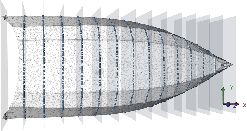

It is clear that the first column of the matrix ${{\bm{P}}}$ which corresponds to the left-most section in Fig. 1 is the result of linear interpolation of points of the left section. This column will mainly represent a geometry which does not exist in the actual object geometry. In the case of concave shapes linear interpolation may lead to introducing non-existing points in the void. Applying the procedure of fitting a NURBS surface to such a matrix ${{\bm{P}}}$ results in the surface shown in Fig. 2 which involves a non-existing portion of the original geometry.

Figure 2.

NURBS surface inadequately representing a non-convex geometry based on parallel sections of initial geometry (Fig. 1).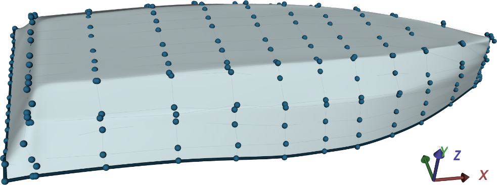

Another problem appears when the projection of surface from one direction (in our case $z$ -direction) is not unique, mathematical speaking not isomorphic. In the example of the sailing boat hull with a stern transom (Fig. 3), the neighboring sections beyond the stern have their respective start and end at a close part of the geometry. Nevertheless, the parallel sections procedure results in closed sections at the transom, which causes two problems. The first is to define the start and end of closed sections such that all starts and ends correspond geometrically. The second, more significant problem, is due to the fact that at the bottom of the transom open and closed sections appear next to each other. This causes a loss of geometric topology, i.e. consecutive points in the matrix ${{\bm{P}}}$ describe completely different portions of the geometry.

Figure 3.

Parallel sections (by parts) of closed geometry – non-isomorphic geometry.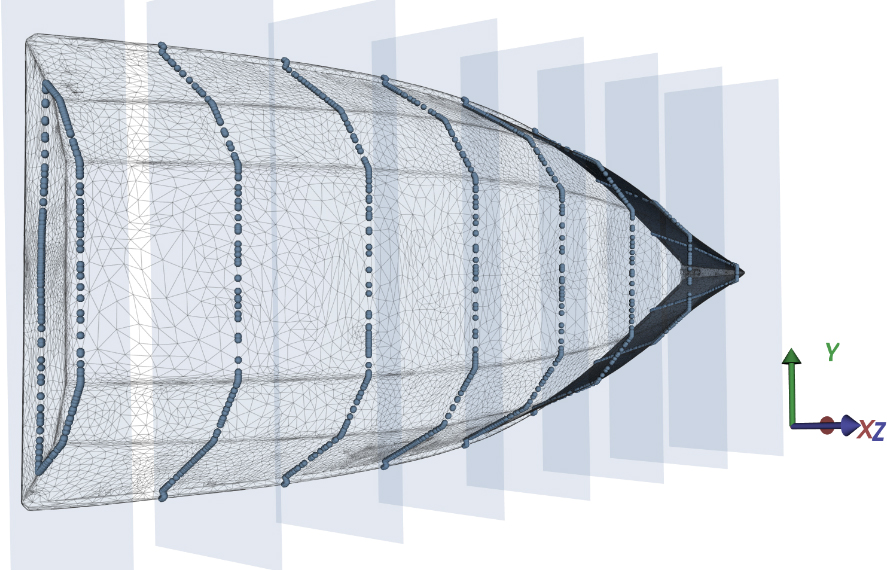

Fitting a NURBS surface to such a matrix ${{\bm{P}}}$ results in the surface shown in Fig. 4 which completely deviates from the original geometry at the transom and the entire stern portion.

Figure 4.

NURBS surface of non-isomorphic geometry based on parallel sections of initial geometry (Fig. 3).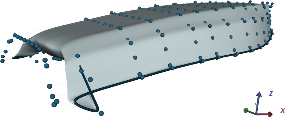

3. Developing the NURBS models

This paper is focused on single-patch parametric surface representations (i.e. NURBS) of complex objects which is of critical importance in engineering shape optimization. An important precondition for an efficient implementation of such a procedure is the initial fitting of the parametric surface to the existing shape given by its geometry. The concept of ‘geometry’ represents a triangulated point cloud obtained by 3D scanning denoted as ${{\bm{\Omega}}}^{{\nabla}}$ .

The NURBS surface is formulated based on $n_{0}\times n_{1}$ control points in ${{\bm{Q}}}$ and the basic functions of degrees ${p_{u},p}_{v}$ denoted by $N_{i_{0},p_{u}}(u)$ and $N_{i_{1},p_{v}}(v)$ ,

$\displaystyle{\bm{C}}\left({\bm{u},\bm{v}}\right)=$ $\displaystyle\frac{\sum\nolimits_{i_{0}=0}^{{n}_{0}}\sum\nolimits_{i_{1}=0}^{{% n}_{1}}{{\bm{N}}_{i_{0},{p}_{{u}}}\left({\bm{u}}\right){\bm{N}}_{i_{1},{p}_{v}% }\left({\bm{v}}\right){\bm{w}}_{i_{0}i_{1}}{\bm{Q}}_{i_{0}i_{1}}}}{\sum% \nolimits_{i_{0}=0}^{{n}_{0}}\sum\nolimits_{i_{1}=0}^{{n}_{1}}{{\bm{N}}_{i_{0}% ,{p}_{{u}}}({\bm{u}}){\bm{N}}_{i_{1},{p}_{v}}({\bm{v}}){\bm{w}}_{i_{0}i_{1}}}}$ $\displaystyle\in\mathbb{R}^{3}$ (1)

The control points matrix ${{\bm{Q}}}$ is structured according to

$\displaystyle{\bm{Q}}=\begin{bmatrix}{\bm{Q}}_{00}&\ldots&{\bm{Q}}_{0n_{1}}\\ \vdots&\ddots&\vdots\\ {\bm{Q}}_{n_{0}0}&\ldots&{\bm{Q}}_{n_{0}n_{1}}\\ \end{bmatrix}\in\mathbb{R}^{3(n_{0}+1)\times(n_{1}+1)}$ (2)

while the matrix ${{\bm{W}}}$ contains the corresponding weight factors accordingly.

The arguments $u$ and $v\in\left[0,1\right]$ map to the vector ${\bm{C}}\left(u,v\right)$ which defines the corresponding point on the NURBS surface.

The intention is here to represent an actual shape by a NURBS surface which implies fitting the surface to the corresponding geometry which needs to have a matrix topology according to Eq. (3).

$\displaystyle{\bm{P}}=\begin{bmatrix}{\bm{P}}_{00}&\ldots&{\bm{P}}_{0∼{}m_{1}}% \\ \vdots&\ddots&\vdots\\ {\bm{P}}_{m_{0}0}&\ldots&{\bm{P}}_{m_{0}m_{1}}\\ \end{bmatrix}\in\mathbb{R}^{3(m_{0}+1)\times(m_{1}+1)}$ (3)

This topology consists of $(m_{0}+1)$ sections of the geometry with $(m_{1}+1)$ points in each. The matrix topology can be obtained by projecting the geometry into a rectangular domain. Simple intersection of the geometry by planes provides points of intersection of the planes and the edges of the triangulated surface. However, this results in unequal numbers of points per section. Figure 5 illustrates this situation using the example of a point cloud obtained by 3D scanning of a small boat hull.

Figure 5.

Parallel sections illustration of 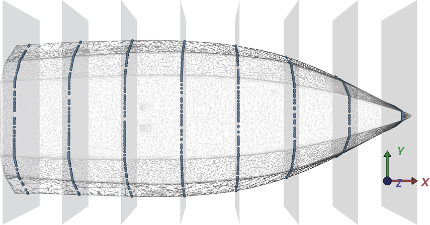${\bm{\Omega}}^{\nabla}$ .

Nevertheless, the structure of the matrix ${{\bm{P}}}$ in Eq. (3) requires all the sections to contain the equal number of points, ( $m_{1}+1$ ). The connectivity of the points of the triangulated surface provides edges, which intersected by the sections represent contours. A simple procedure is feasible to select ${(m}_{1}+1)$ points for each section from the points of the contour.

The matrix data-set topology in Eq. (3) can be obtained by choosing new ( $m_{1}+1$ ) points located on the original section.

With $\left\{{\bm{P}}_{i}^{O}\right\}_{i=0}^{n}$ being the original ( $n+1$ ) points of the $k$ -th 3D section (contour) after intersecting the initial shape, and $\left\{{\bm{P}}_{k}^{C}\right\}_{k=0}^{m_{1}}$ the new $(m_{1}+1)$ points at the same contour, then for a new point ${\bm{P}}_{k}^{C}$ .

An $i$ exists such that ${\bm{P}}_{k}^{C}\in\left[{\bm{P}}_{i}^{O},{\bm{P}}_{i+1}^{O}\right]$

$\displaystyle\sum_{j=0}^{i-1}\left\|{\bm{P}}_{j+1}^{O}-{\bm{P}}_{j}^{O}\right% \|+\left\|{\bm{P}}_{i}^{O}-{\bm{P}}_{k}^{C}\right\|$ $\displaystyle=k\frac{\sum_{j=0}^{n-1}\left\|{\bm{P}}_{j+1}^{O}-{\bm{P}}_{j}^{O% }\right\|}{m_{1}+1},$ (4)

which provides the new ${(m}_{1}+1)$ equi-distant (in curvilinear coordinates) points $\left\{{\bm{P}}_{k}^{C}\right\}_{k=0}^{m_{1}}$ .

In Eq. (4), the interval where the point ${\bm{P}}_{k}^{C}$ belongs is determined by a simple procedure such that ( $i-1$ ) whole intervals and partially the $i$ -th are aggregated.

Fitting a NURBS surface to the geometry matrix ${{\bm{P}}}$ correlates parameter values $u_{j_{0}j_{1}}$ , $v_{j_{0}j_{1}}\in[0∼{}∼{}1]$ and points ${\bm{P}}_{j_{0}j_{1}}$ such that

${{\bm{C}}(u}_{j_{0}j_{1}},v_{j_{0}j_{1}})\to{\bm{P}}_{j_{0}j_{1}}$ (5)

${{\bm{C}}(u}_{j_{0}j_{1}},v_{j_{0}j_{1}})$ being the point on the NURBS surface.

Fitting the NURBS surface to the geometry matrix ${{\bm{P}}}$ is a least-squares problem in minimizing the error function

$\displaystyle{\bm{E}}\left({\bm{U},\bm{V},\bm{Q},\bm{W}}\right)=$ $\displaystyle\frac{1}{2}\sum_{{j}_{0}=0}^{{m}_{0}}\sum_{{j}_{1}=0}^{{m}_{1}}% \left\|\bm{C}(\bm{u}_{{j}_{0}{j}_{1}},{\bm{v}}_{{j}_{0}{j}_{1}})-{\bm{P}}_{{j}% _{0}{j}_{1}}\right\|^{2}$ (6)

The proposed formulation of the fitting procedure Eq. (3) developed by the authors augments the problem by introducing the matrices of parameter values ${{\bm{U}}}$ and ${{\bm{V}}}$ as additional best-fitting variables beyond the commonly used control points ${{\bm{Q}}}$ and homogeneous terms ${{\bm{W}}}$ .

The number of control points and the homogenous terms in Eq. (3) is $\left(n_{0}+1\right)\times\left(n_{1}+1\right)$ and hence the number of the best-fitting variables is not too high. On the other hand, the size of ${{\bm{P}}}$ is commonly very large resulting in correspondingly large ${{\bm{U}}}$ and ${{\bm{V}}}$ matrices. Including all elements of the ${{\bm{U}}}$ and ${{\bm{V}}}$ matrices as best-fitting variables is therefore not acceptable. Moreover, any change in ${{\bm{U}}}$ and ${{\bm{V}}}$ must preserve ordered sequences of values as otherwise geometric singularity would occur. Instead of including all elements of ${{\bm{U}}}$ and ${{\bm{V}}}$ as independent variables, the approach developed by the authors sets entire columns and rows to the same respective value. This leads to vectors ${{\bm{u}\in\mathbb{R}}}^{m_{0}+1}$ and ${{\bm{v}\in\mathbb{R}}}^{m_{1}+1}$ of acceptable size.

The Levenberg-Marquardt method is applied for the resulting enhanced best-fitting problem with ${\bm{u},\bm{v},\bm{Q}}$ and ${\bm{W}}$ as the respective variables.

Best-fitting a NURBS surface to the boat hull point cloud using ${\bm{u},\bm{v},\bm{Q}}$ and ${\bm{W}}$ as best-fitting variables according to Eq. (3) is illustrated in Fig. 6.

More details about the proposed parametric model and its applications can be found in Ćurković et al. [8].

Figure 6.

Best-fitting according to Eq. (3) for the boat hull example.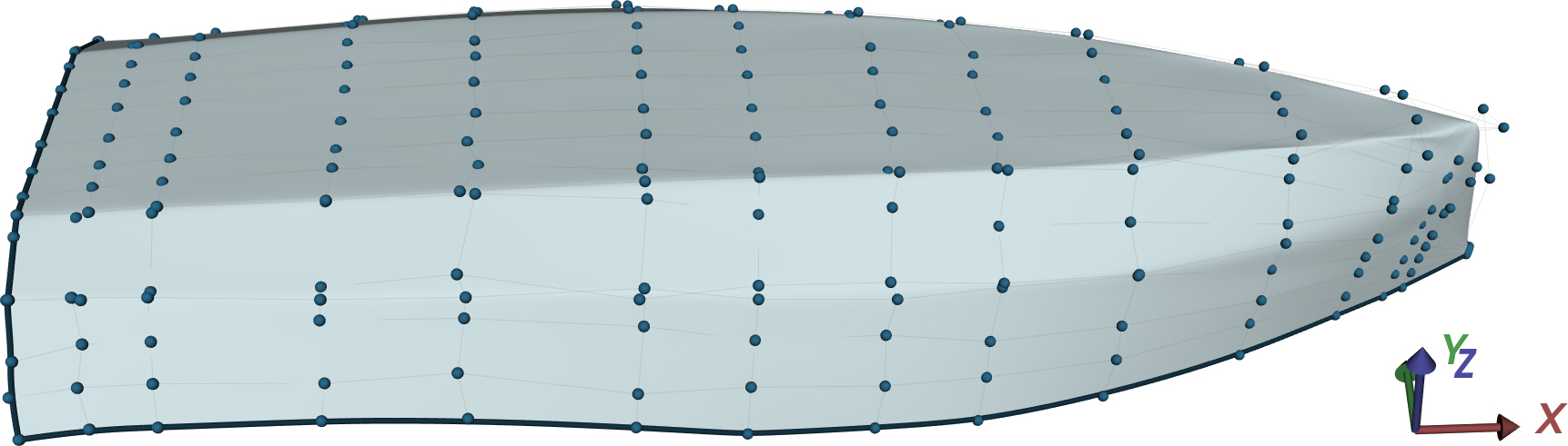

4. The proposed projecting method

The geometry matrix ${{\bm{P}}}$ is not always easy to obtain from point clouds in the way demonstrated in Fig. 5 by applying parallel sections of the original surface mesh geometry. Applying sections to the original geometry in order to construct the matrix ${{\bm{P}}}$ is only viable if the original geometry is convex and smooth, without ‘stepwise’ local changes in shape. The geometric topology of ${{\bm{P}}}$ corresponds to the topology of the fitted parametric surface only for such ‘simple’ shapes.

The following section of the paper develops a procedure of projecting the geometry into a rectangular domain. This approach avoids the problems demonstrated above and also contributes to the numerical quality of the fitting procedures developed earlier.

The proposed method is based on algorithms from graph theory and consists of a sequence of steps described next and accompanied by Fig. 7 where the convex geometry of sailing boat hull without transom is chosen for demonstration.

Figure 7.

The developed procedure of projection into a rectangular domain. (a) Geometry of sailing boat hull without transom (to be projected); (b) Projection into rectangular domain.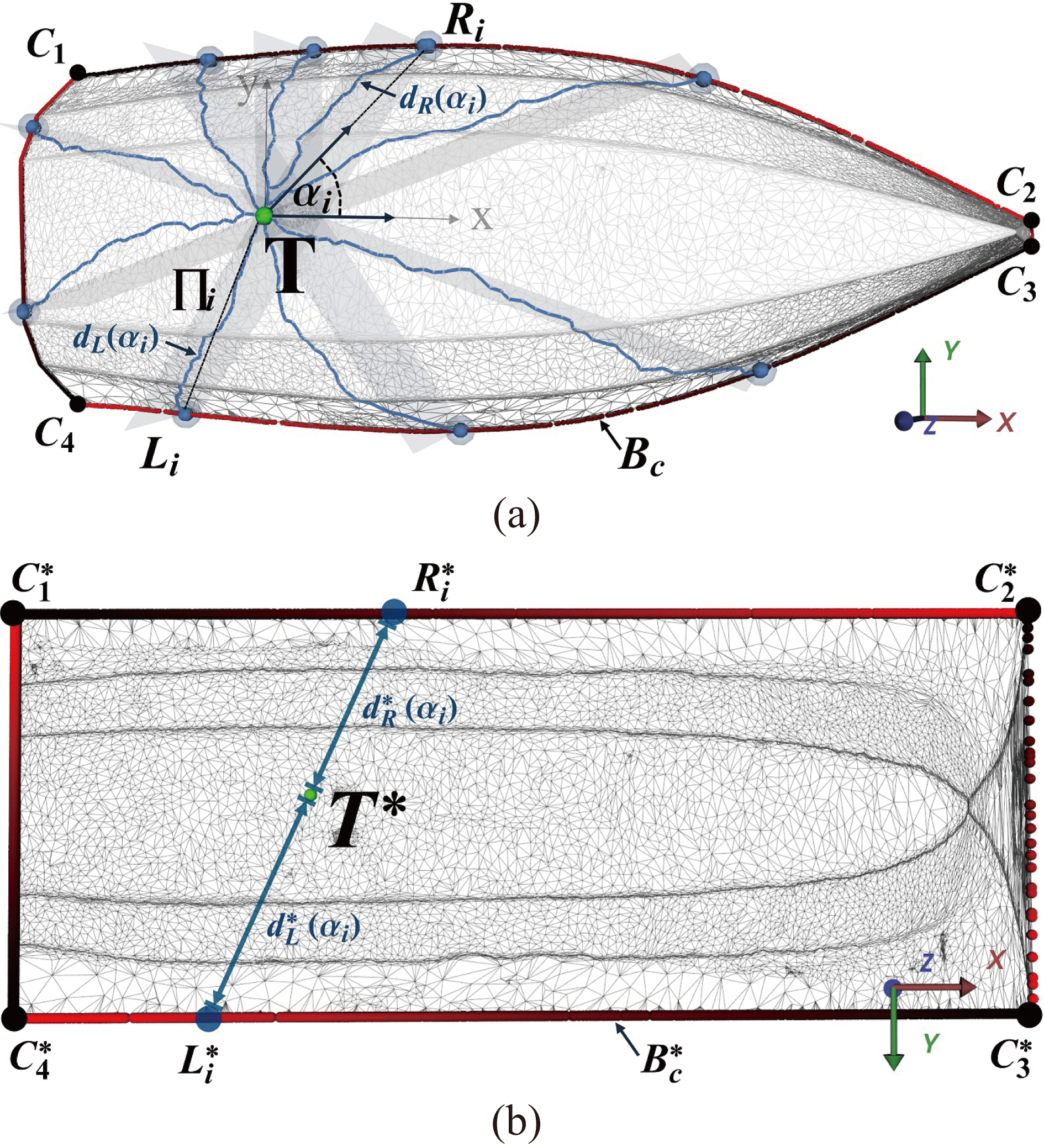

With the definition of an undirected graph as a pair of sets ( $V, E$ ), where elements of the set $V$ are called nodes (vertex, node or point), and those in set $E$ bridges (often referred to as branches, edges or links), the steps of the proposed method can be structured according to the following sequence:

viii. i.

As first, the boundary contour is extracted - points denoted as ${\bm{B}}_{c}$ .

ii.

Four key points of the boundary contour ${\bm{C}}_{1}$ ${-}$ ${\bm{C}}_{4}$ are extracted, the projections of which ${\bm{C}}_{1}^{*}$ ${-}$ ${\bm{C}}_{4}^{*}$ will constitute a rectangular domain. The absolute positions of the points ${\bm{C}}_{1}^{*}$ ${-}$ ${\bm{C}}_{4}^{*}$ are insignificant (in this case of the boat hull we chose the projection domain to be $[0,2]$ $\times$ $[0,1]$ for better presentation).

iii.

In the third step, the boundary contour is projected between the respective corner points. The spacing of the ${\bm{B}}_{{C}}^{{*}}$ points in the projection domain between the respective corner points is linearly correlated to the physical distances between the points ${\bm{B}}_{c}$ .

iv.

For each point ${{\bm{T}}}$ of the interior1 surface $V^{I}$ , the respective shortest distances to all the points of the boundary contour are identified and stored in the matrix ${\bm{D}}\in\mathbb{R}^{\left|V^{I}\right|\times\left|{\bm{B}}_{c}\right|}$ , where $\left|V^{I}\right|$ is the total number of points of the interior and $\left|{\bm{B}}_{c}\right|$ the number of points of the boundary contour ${\bm{B}}_{c}$ .

For a given number of sections $n$ , using a set of given angles $\alpha_{i}=i*\frac{2\pi}{n},$ where $i=1,\ldots,n$ , and the plane ${\bm{\Pi}}$ given by the equation

$\bm{\Pi}:y=0$

for each point ${{\bm{T}}}$ of the interior of the geometry, the associated set of pairs of 3D points

${\bm{S}}=\left\{\left({\bm{L}}_{i},{\bm{R}}_{i}\right):{\bm{\Pi}}_{i}={\bm{\Pi% }}\text{∼{}rotated by∼{}}\alpha_{i}\right\}$

is determined such that the plane ${\bm{\Pi}}$ is rotated by the angle $\alpha_{i}$ thereby cutting the boundary contour. The set ${\bm{S}}$ contains points where the plane ${\bm{\Pi}}_{i}$ cuts the boundary contour at two places. In the case when the boundary contour is not convex and the plane ${\bm{\Pi}}_{i}$ cuts it in more than two places, we take in consideration just the two closest intersection points which are in opposite sides from the point ${{\bm{T}}}$ . The number of cuts $n$ is chosen arbitrarily based on experience.

vi.

Graphical distances from point ${{\bm{T}}}$ to the points ${\bm{L}}_{i}$ and ${\bm{R}}_{i}$ are denoted as $d_{i}^{L}$ and $d_{i}^{R}$ . The set ${{\bm{S}}}$ generally does not correspond to vertices of the edge contour. Hence, based on the vertices of the edges which contain ${\bm{L}}_{i}$ and ${\bm{R}}_{i}$ , the values $d_{i}^{L}$ and $d_{i}^{R}$ are calculated as average values of the shortest paths from the point ${{\bm{T}}}$ to the vertices of the edges intersected by ${\bm{L}}_{i}$ and ${\bm{R}}_{i}$ .

vii.

The projection ${\bm{L}}_{i}^{*}$ and ${\bm{R}}_{i}^{*}$ of the intersection points ${\bm{L}}_{i}$ and ${\bm{R}}_{i}$ are projected between the respective corner points the same way as boundary contour points.

viii.

The position of the projection of a point ${{\bm{T}}}$ from the interior of the rectangular domain is finally given by:

$\displaystyle{\bm{T}}^{*}=\frac{1}{n}\sum\limits_{i=0}^{n}\left(d_{i}^{L*}{\bm% {L}}_{i}^{*}+d_{i}^{R*}{\bm{R}}_{i}^{*}\right),$ (7)

where $d_{i}^{L*}=\frac{d_{i}^{L}}{d_{i}^{L}+d_{i}^{R}}$ and $d_{i}^{R*}=\frac{d_{i}^{R}}{d_{i}^{L}+d_{i}^{R}}$ respectively.

The main complexity of the proposed method is due to the step (iv), where for each point of the interior surface ( $V^{I}$ ) the shortest distances to all the points of the boundary contour ( ${\bm{B}}_{c}$ ) are identified and stored in the matrix ${\bm{D}}\in\mathbb{R}^{\left|V^{I}\right|\times\left|{\bm{B}}_{c}\right|}$ . While Dijkstra’s and Bellman-Ford’s algorithms of all-pairs shortest path problem run in $O(\left|V\right|^{3})$ time, where $\left|V\right|$ is the number of all points of the geometry, the reduced problem of the proposed step (iv) runs in $O(\left|V^{I}\right|^{2}\cdot\left|{\bm{B}}_{c}\right|)$ . Since the number of points of the interior $\left|V^{I}\right|<\left|V\right|$ and the number of points of the boundary contour $\left|{\bm{B}}_{c}\right|\ll\left|V\right|$ , it is expected that the proposed reduced problem has lower algorithm complexity than the global Dijkstra’s and Bellman–Ford’s algorithms. Despite that somewhat reduced complexity of the most demanding step of the proposed algorithm, it is still a major drawback with respect to other algorithms [3, 21, 33, 44, 47] which are linear problems. Nevertheless, in those cases where the information pertaining to shortest paths already exist, the proposed projection method can be used without any doubts in its successfulness.

Like other methods of 2D projection, the proposed method also uses four key points to constitute a rectangular domain. In theory, the projection could be done with three points, but in that case it would give up the parametric topology resulting from the integral parametric models (NURBS, …). The ‘good’ parametric topology implies that the control points of the parametric model exhibit impact on geometrically equally demanding areas. In the case with only three key points this is not case because one of the three key points is represented by a whole column/row of control points. That situation would cause bias for some part of the geometry, which would in optimization terms lead to local optima which is not numerically acceptable.

The final calculation for each projected point includes averaging values of $n$ projected pairs of boundary points. For the examples in this paper, the value of $n$ was set to 100. We also used higher values of $n$ from 100 to 5000, but the version of 100 sections proved to be accurate enough. Theoretically, instead of 100 or more sections only the four key corner points ${\bm{C}}_{1}$ ${-}$ ${\bm{C}}_{4}$ are needed for the projection of each interior point. However, a small number of sections produced a disorderly projected geometry with overlapping triangles, especially in cases of low density of the original geometry. Such a projection of the geometry results in an irregular matrix form of the initial geometry and ultimately in divergence of the optimization process of fitting.

5. Results and discussion

Using parallel sections with the rectangular domain (Fig. 8a) provides points whose values are replaced by corresponding points of the original geometry by virtue of geometric topology. This procedure enables the entire geometry to be embraced, and the geometric topology of the sections provides an excellent initial solution for fitting procedures.

Figure 8.

Corresponding sections in rectangular domain and original geometry. (a) Sections in the rectangular domain; (b) Sections in the original geometry.

The following two examples demonstrate successful fitting of the NURBS surface after projecting into a rectangular domain according to the method developed in this paper. Figure 9 shows that the concave part of geometry is not a problem any longer by virtue of the developed procedure, and the curvature from the left to right side is gradual which is important in terms of convergence of the fitting process.

Figure 9.

Sailing boat, partial hull with concave geometry: (a) projection into rectangular domain; (b) NURBS surface 15 $\times$ 20 CPs, both directions 3 ${}^{\rm rd}$ degree.

Figure 10.

Sailing boat hull with transom. (a) Proposed projection into rectangular domain; (b) NURBS surface 15 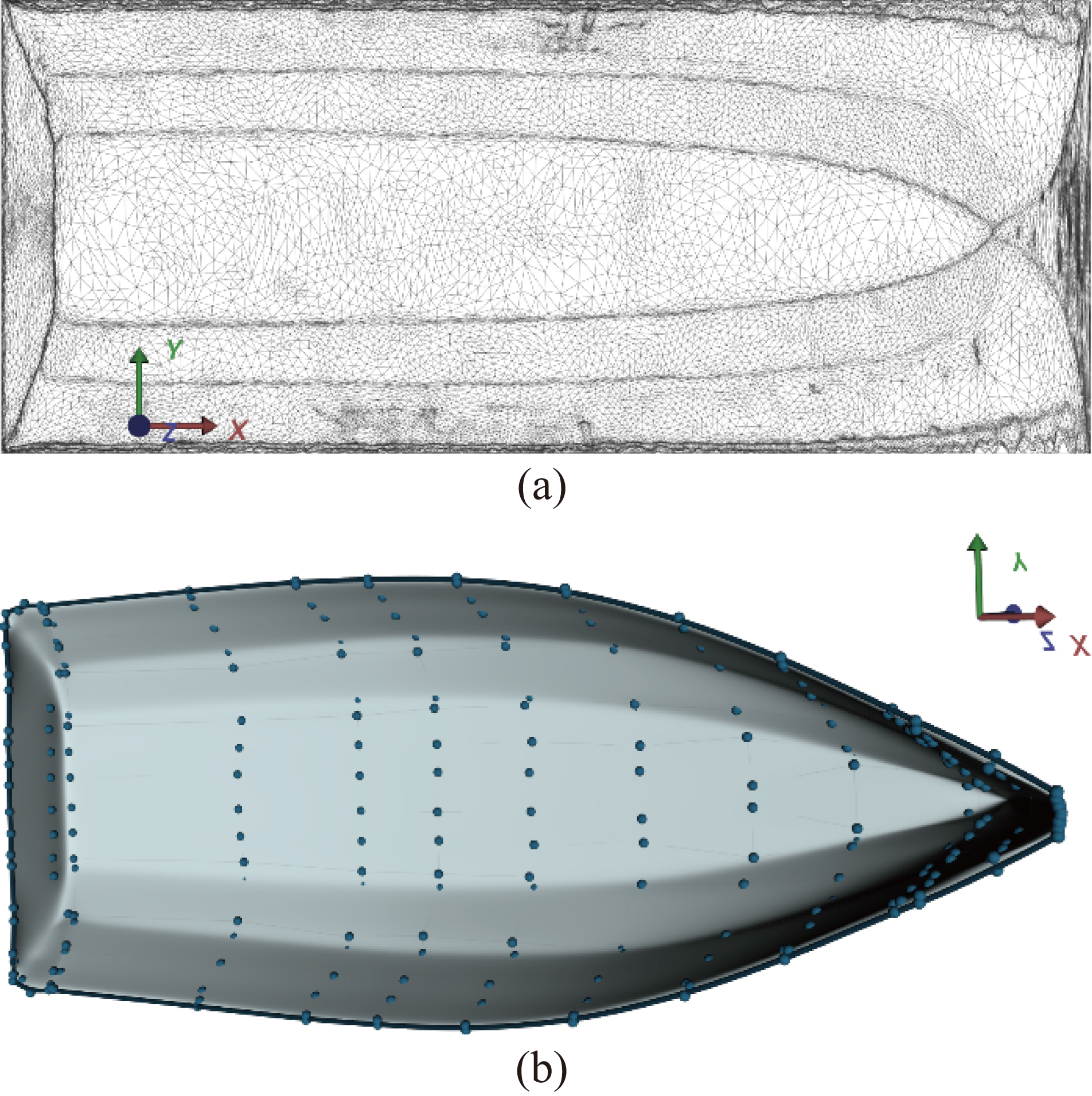$\times$ 20 CPs, both directions 3 ${}^{\rm rd}$ degree.

Figure 11.

The developed procedure applied to the shell of the student formula racing car. (a) Point cloud after optical 3D scanning of student’s formula student shell; (b) Proposed projection into rectangular domain; (c) NURBS surface, 20 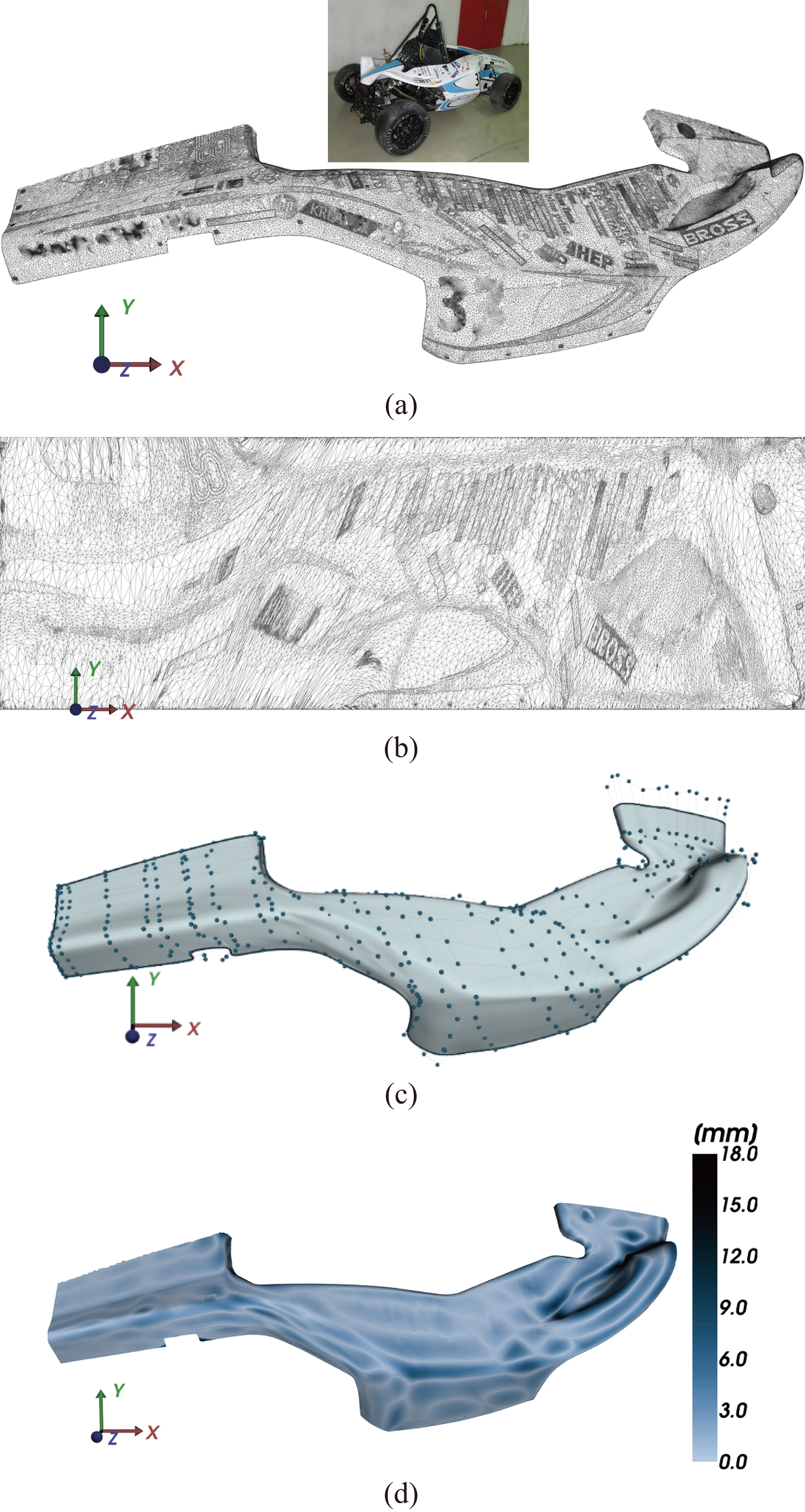$\times$ 15 control points, both directions 3 ${}^{\rm rd}$ degree; (d) Error distribution – difference between original model ( ${\mathbf{\Omega}}^{{\nabla}}$ ) and NURBS surface.

The next example (Fig. 10) demonstrates the successful fitting of an integral NURBS model on the non-isomorphic geometry implemented by the proposed projecting method. The possibility of fitting such a geometry using a single-patch NURBS model (instead of the common multi-partition approach) is highly welcome in shape optimization, where the geometric model may be exposed to significant change during the course of iterations in optimization quasi-time.

Another demanding test-case of a complex geometry where it is virtually impossible to fit a single-patch parametric model without projecting into a rectangular domain is the formula-student shell as shown in Fig. 11. Projecting the respective geometry into a rectangular domain according to the procedure developed in Section 4 makes this complex single-patch fitting problem viable.

In order to demonstrate how the developed procedure can be applied for closed geometries (in literature also called ‘watertight’), we chose the numerically generated example of spheres emerging from a cube, Fig. 12.

Figure 12.

Parametrization of closed geometry – numerically generated sample. (a) Closed geometry; (b) The bottom part of the geometry (a); (c) Projection into rectangular domain of (b); (d) NURBS surface of (b) using (c), 35 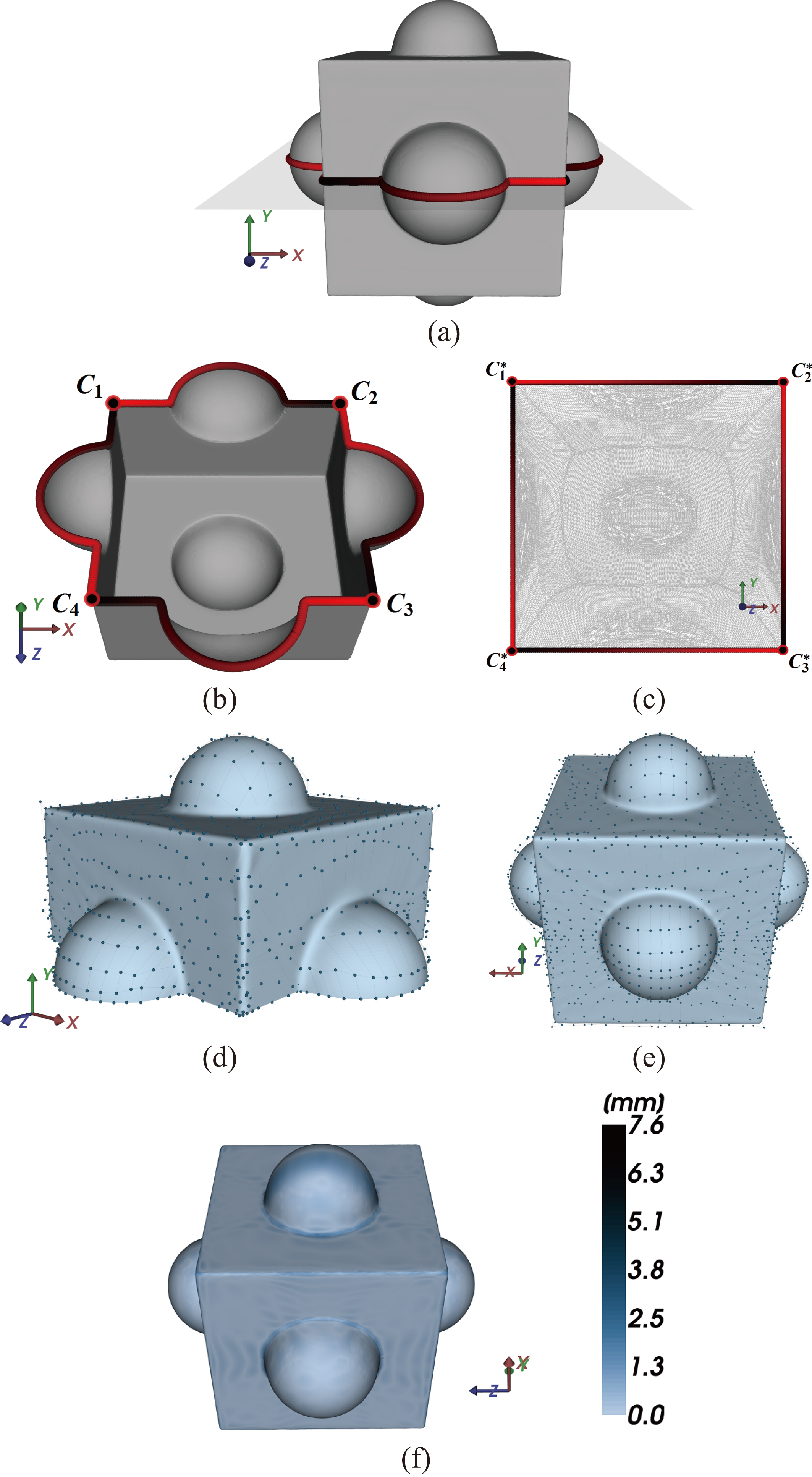$\times$ 35 control points, both directions 3 ${}^{\rm rd}$ degree; (e) Two connected NURBS surfaces: (d) and NURBS surface of opposite side of (b); (f) Error distribution – difference between (a) and (e).

The generated geometry (Fig. 12a) is subdivided by a plane in two separated parts. Each part (Fig. 12b shows the bottom part) is projected into a rectangular domain (Fig. 12c shows the bottom part) and parameterized using a NURBS surface (Fig. 12d shows the bottom part). To make a complete NURBS model of the initial geometry, we just connect the two separate NURBS surfaces into a global one (Fig. 12d). This way there is no bias for any part of the geometry and the control points of NURBS surface are equally distributed. In the above example, continuity is not explicitly provided for as it is not in the focus here.

With respect to the proposed approach with two separate parameterizations based on projection into a rectangular domain, Fig. 13 shows the parametrization of the same closed geometry (Fig. 12a) based on the matrix form of geometry obtained by standard intersecting from a pole.

Figure 13.

Parametrization of closed geometry using intersecting from a pole. (a) Matrix form of the geometry obtained by intersecting from a pole at different angles; (b) Single NURBS surface of (a), 50 $\times$ 50 control points, both directions 3 ${}^{\rm rd}$ degree; (c) Error distribution – difference between (a) and (b).

It is obvious that this way of generating the matrix form of the geometry generates bias in the distribution of the control points. In areas around the chosen pole(s) there is dense distribution of the control points (front part of Fig. 13b), while in other parts of the geometry there are insufficient control points to represent the geometry in a satisfactory way (top part of Fig. 13b).

The next figure, Fig. 14, shows the possibility of projecting into a rectangular domain of a geometry with a hole. In order to generate a single-part connected boundary contour, the geometry is intersected between the inside and outside circle of the boundary. The four key boundary contour points lie at the ends of the intersection line and they are set as ${\bm{C}}_{1}={\bm{C}}_{4}$ and ${\bm{C}}_{2}={\bm{C}}_{3}$ respectively.

Figure 14.

Selection of the boundary contour of geometry with included hole. (a) Geometry including a hole; (b) Boundary contour with key four points.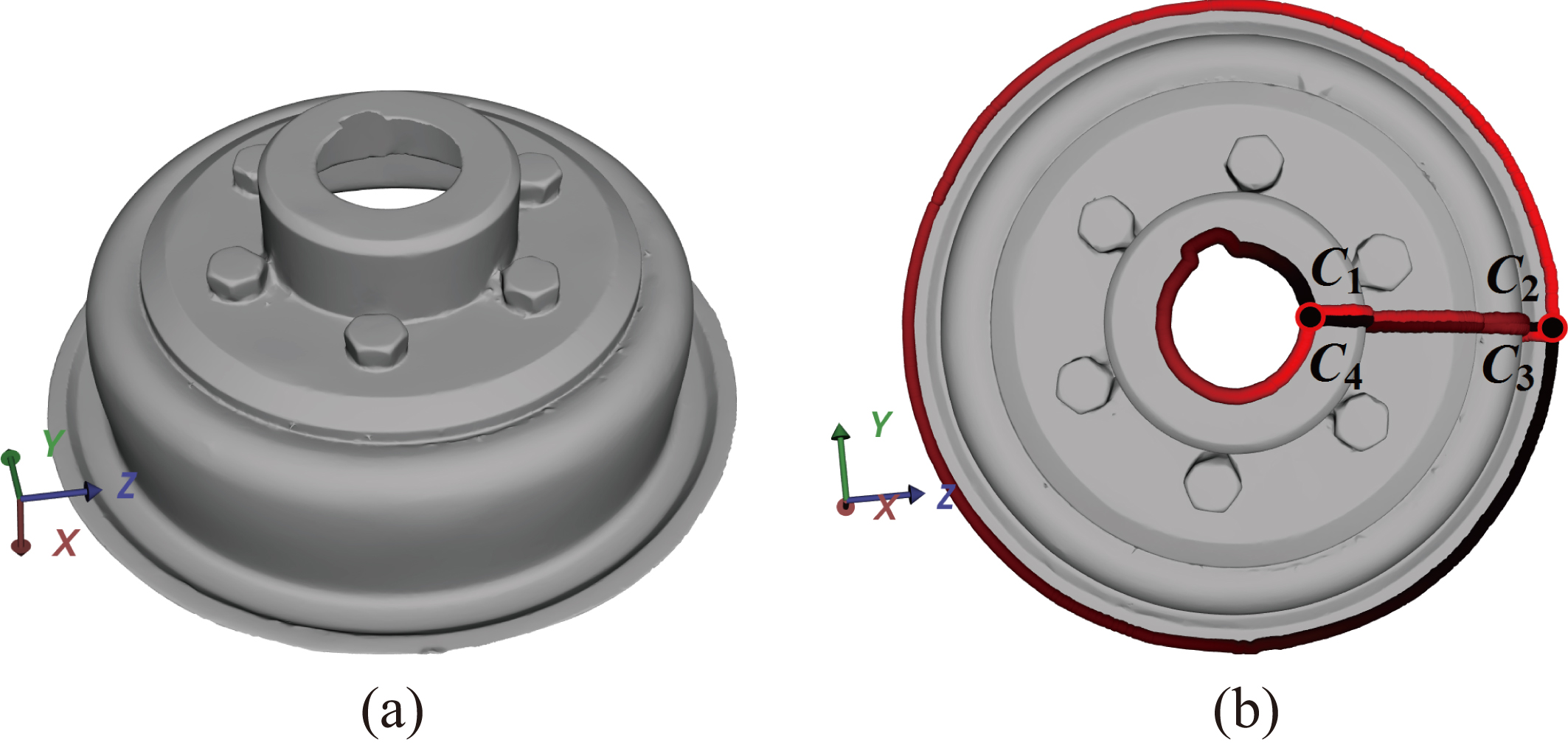

Figure 15.

Spring analogy method – projecting geometry of sailing boat hull into a rectangular planar domain. (a) Projected geometry; (b) NURBS surface 15 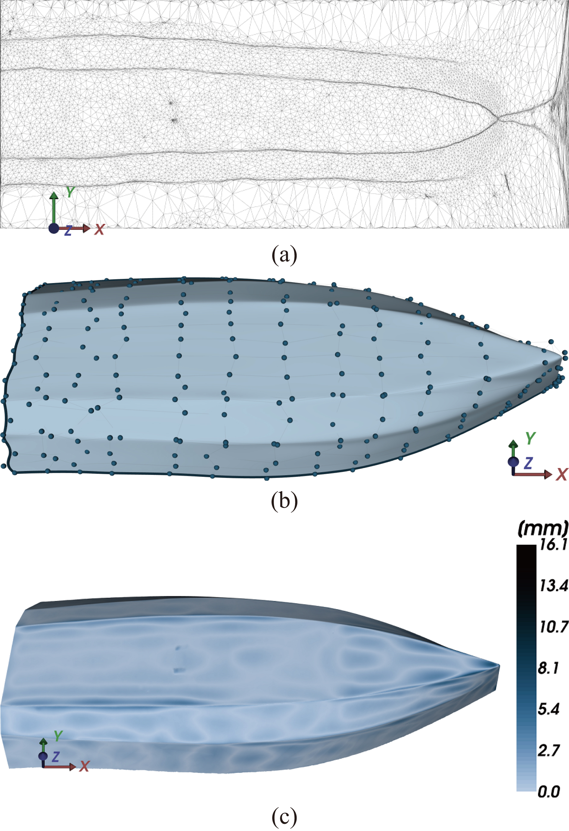$\times$ 20 control points, both directions 3 ${}^{\rm rd}$ degree; (c) Error distribution – difference between original model ( ${{\bm{\Omega}}}^{{\nabla}}$ ) and NURBS surface.

5.1 Comparison with other methods

We also implemented projections of the sailing boat hull test-case using two other projection methods: method based on spring analogy [3] and the widely used harmonic projection [16], both shown in the figures bellow, Figs 15 and 16.

Table 1
The computational stretch

Model	Spring analogy	Harmonic	Proposed
Sailing boat hull	3.508210	2.579464	2.666498
Formula student shell	2.361398	1.814427	2.300568

Table 2

The computational shear

Model	Spring analogy	Harmonic	Proposed
Sailing boat hull	0.372217	0.127836	0.165685
Formula student shell	0.770783	0.774135	0.496487

Figure 16.

Harmonic projecting – projecting geometry of sailing boat hull into a rectangular planar domain. (a) Projected geometry; (b) NURBS surface 15 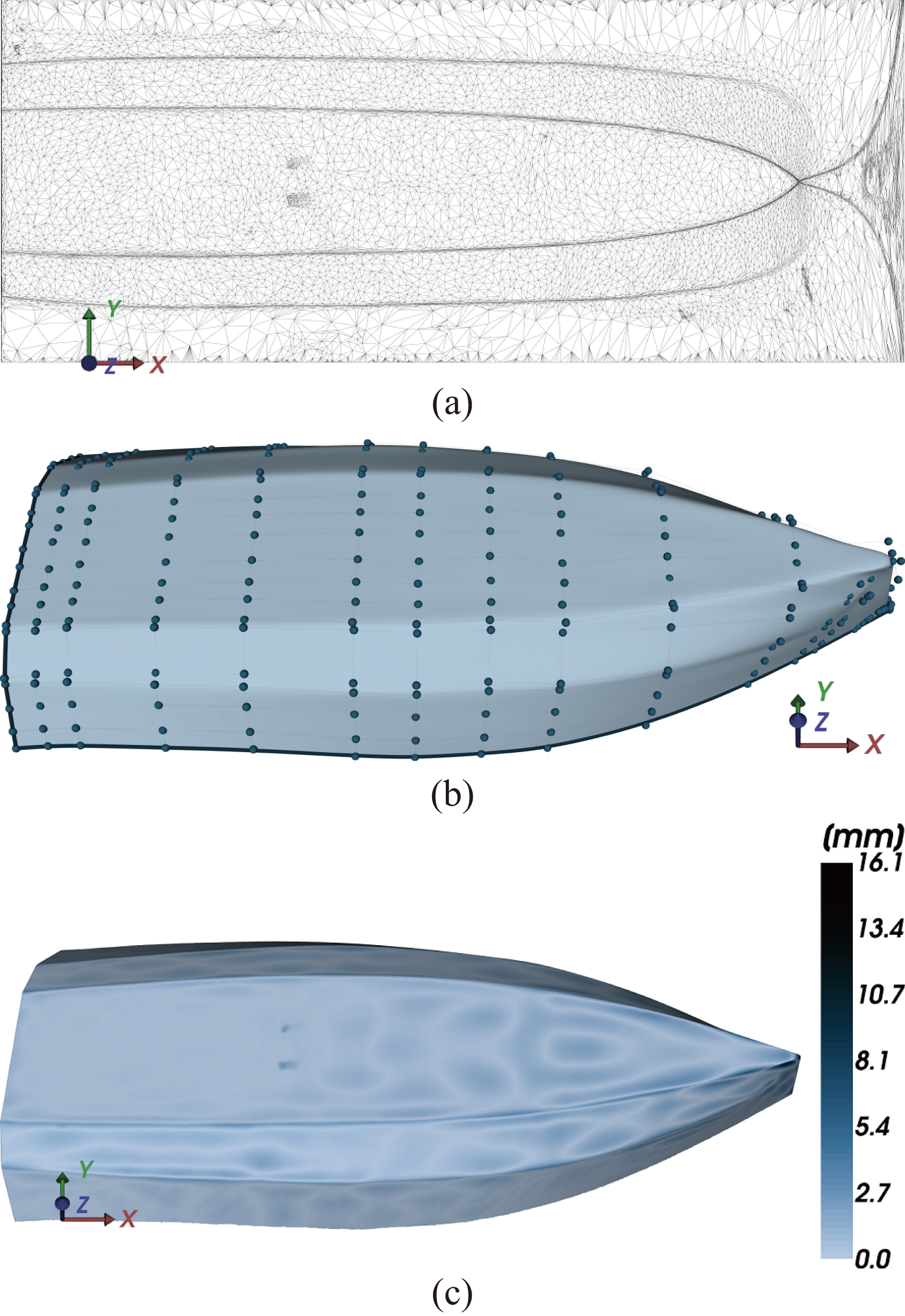$\times$ 20 control points, both directions 3 ${}^{\rm rd}$ degree; (c) Error distribution – difference between original model ( ${{\bm{\Omega}}}^{{\nabla}}$ ) and NURBS surface.

The method with a spring analogy (Fig. 15) results in a slightly wrinkled mesh. Since this effect is transitive, the matrix form Eq. (3) of the geometry can also become wrinkled. This appearance directly affects the positioning of control points of the parametric model, which in terms of shape optimization causes worse convergence properties. The wrinkling effect of the projected mesh is more pronounced for geometries where significant difference in size is present for adjacent triangles. On the other side, the projected mesh created by harmonic projection, Fig. 16, completely keeps the topological features from the original geometry and behaves wrinkle-free. The result of the proposed method is illustrated in Fig. 17.

Table 3

Computational time in seconds

Model	Spring analogy	Harmonic	Proposed
Sailing boat hull	3.01	3.28	117
Formula student shell	1.220	1.352	24.3

Figure 17.

Proposed method – projecting geometry of sailing boat hull into a rectangular planar domain. (a) Projected geometry; (b) NURBS surface 15 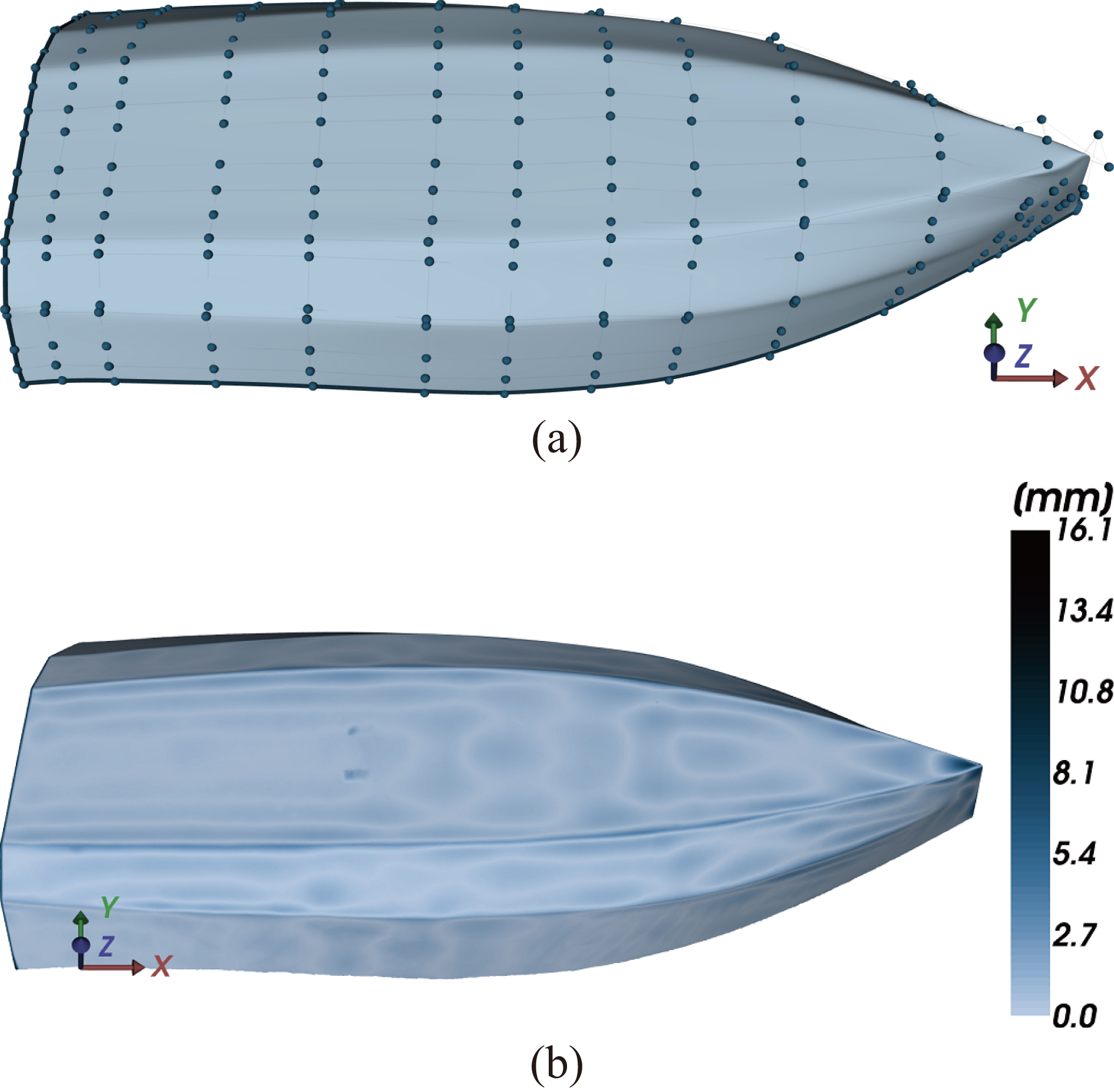$\times$ 20 control points, both directions 3 ${}^{\rm rd}$ degree; (c) Error distribution – difference between original model ( ${{\bm{\Omega}}}^{{\nabla}}$ ) and NURBS surface.

We use two metrics to measure the parametric distortion. Using the same formula as Sander et al. [36] we give the $L_{2}$ stretch (lengthwise deformation) error and for $L_{2}^{\textit{shear}}$ as the measure of conformality we use the same formula as Sheffer et al. [44].

The next table presents the computational time for the same examples.

6. Conclusion

This paper develops a method for projecting geometries of 3D objects into rectangular domains, for example for point clouds obtained by optical surface scanning. The developed approach makes it possible to obtain well-structured geometry matrices even for complex-shape objects, thereby preserving the original topology. The developed approach solves the problems related to non-isomorphic geometries and those involving concave portions. The proposed method can qualitatively be compared with the spring-mesh and harmonic projection procedures. Unlike the former, the developed method does not generate wrinkling, and may perform similarly to the latter if the shortest-path information exists for the internal mesh points. Generally however, the method is more computationally-intensive in most cases as it involves a multitude of shortest-path sub-problems.

Future work related to the developed procedure will proceed in several directions. The parameterization approach will be tested using complex geometries of engineering objects both in terms of single-patch models and multi-partition models. Within the framework of shape optimization, the procedure will also be evaluated in demanding cases of dynamically changing geometric topologies (as imposed by the shape optimizer). In such cases edges may disappear and arise, thereby also changing the partitioning schemes. In future work, in order to deal with 3D big data, we plan to enhance the proposed method using efficient geometric algorithms and GPU-based computation.

Footnotes

Interior surface $V^{I}$ – triangulated surface without the boundary contour

Acknowledgments

This work was supported by the Croatian Science Foundation [grant number IP-2014-09-6130].

Appendix A

The following is the key part of the proposed pseudo code for calculating the shortest distances for each point of the interior ( ${\bm{V}}^{{I}}$ ) to all the points of the boundary contour ( ${\bm{B}}_{{c}}$ ). The distances are identified and stored in the matrix ${\bm{D}}\in\mathbb{R}^{{V}^{{I}}\times E}$ . In order to reduce the algorithm complexity, the calculations of the matrix ${\bm{D}}$ are split into a given number of threads (nThread), thereby reducing the execution time almost by the factor nThread. Sharing the job into threads is implemented by randomly splitting the indices of interior nodes $V^{I}$ into a number of threads. The corresponding indices are stored into associated indices vectors (idsThread) of each thread.

The overall proposed procedure is shown in Algorithm 1.

Algorithm 1. Calculating the shortest distances for each point of the interior ( ${\bm{V}}^{{I}}$ ) to all the points of the boundary contour ( ${\bm{B}}_{{c}}$ )

Input:

•

Matrix ${\bm{D}}\in\mathbb{R}^{|V^{I}|\times\left|{\bm{B}}_{{c}})\right|}$ with infinite values;

•

Connections from each interior point to its neighbors: nConn;

•

Distances from each interior point to its neighbors: nDist;

Output: Distances stored in matrix ${{\bm{D}}}$ .

begin

•

Sharing the job into threads by splitting the indices of interior nodes $V^{I}$ into threads: idsThread;

for all threads do

while newChange $=$ 1 //Indicator whether

better path found

newChange $=$ 0

for all indices i in idsThread

for all neighbor nodes nn of i

for all boundary contour nodes bc

if (D[i][bc] $+$ nDist[nn] $<$ D[nConn[nn]][nn]) do

D[nConn[nn]][nn] $=$ D[i][bc] $+$ nDist[nn];

newChange $=$ 1 //Better path found

end if

end for

end while

end for

return ${{\bm{D}}}$ ;

end

Due to splitting the calculation into threads by indices there is a possibility of loosing global connectivity. Consequently, we cannot be sure that the shorthest paths in the matrix ${\bm{D}}$ correspond to actual shorthest paths. Hence, when all threads are finished, we repeat the job with only one thread which includes all indices which assures that ${\bm{D}}$ really corresponds to the aspired data. The number of iterations in the last global thread depends on the number of threads. For the examples in this paper we used a 2.4 Ghz Intel Core i7 machine (4 cores/8 threads).

We also tried machines with less and with more cores/threads, but for proposed examples the optimum was 8 cores. Fewer cores means increasing the job per each thread, but the last global thread with all indices is almost unemployed. On the other hand, in the case with many cores, the job per each thread is not extensive, but because of weak connectivity, the last global thread needs to do almost the full initial problem.

References

Adeli

Cheng

. Concurrent genetic algorithms for optimization of large structures. J Aerosp Eng [Internet]. 1994 Jul; 7(3): 276-96. Available from: http://ascelibrary.org/doi/10.1061/%28ASCE%290893-1321%281994%297%3A3%28276%29.

Adeli

Kumar

. Concurrent structural optimization on massively parallel supercomputer. J Struct Eng [Internet]. 1995 Nov; 121(11): 1588-97. Available from: http://ascelibrary.org/doi/10.1061/%28ASCE%290733-9445%281995%29121%3A11%281588%29.

Becker

Schãfer

Jameson

. An advanced NURBS fitting procedure for post-processing of grid-based shape optimizations. 49th AIAA Aerospace Sciences Meeting including the New Horizons Forum and Aerospace Exposition [Internet]. Reston, Virigina: American Institute of Aeronautics and Astronautics. 2011. Available from: http://arc.aiaa.org/doi/10.2514/6.2011-891.

Böhm

Farin

Kahmann

. A survey of curve and surface methods in CAGD. Comput Aided Geom Des [Internet]. 1984 Jul; 1(1): 1-60. Available from: http://linkinghub.elsevier.com/retrieve/pii/0167839684900037.

Campbell

Flynn

. A survey of free-form object representation and recognition techniques. Comput Vis Image Underst [Internet]. 2001 Feb; 81(2): 166-210. Available from: http://linkinghub.elsevier.com/retrieve/pii/S1077314200908890.

Campomanes-Álvarez

Cordón

Damas

. Evolutionary multi-objective optimization for mesh simplification of 3D open models. Integr Comput Aided Eng. 2013; 20(4): 375-90.

Choi

GPT

Rycroft

. Density-equalizing maps for simply-connected open surfaces [Internet]. 2017. Available from: http://arxiv.org/abs/1704.02525.

Ćurković

Vučina

Ćurković

. Enhanced 3D parameterization for integrated shape synthesis by fitting parameter values to point sets. Integr Comput Aided Eng. 2017; (24): 241-260.

Deb

Goel

. Multi-objective evolutionary algorithms for engineering shape design. Evolutionary Optimization [Internet]. Boston: Kluwer Academic Publishers. 2000; 147-75. Available from: http://link.springer.com/10.1007/0-306-48041-7_6.

10.

Dimitri

De Lorenzis

Scott

Wriggers

Taylor

Zavarise

. Isogeometric large deformation frictionless contact using T-splines. Comput Methods Appl Mech Eng [Internet]. 2014 Feb; 269: 394-414. Available from: http://linkinghub.elsevier.com/retrieve/pii/S0045782513002971.

11.

Dimitri

De Lorenzis

Wriggers

Zavarise

. NURBS- and T-spline-based isogeometric cohesive zone modeling of interface debonding. Comput Mech [Internet]. 2014 Aug 20; 54(2): 369-88. Available from: http://link.springer.com/10.1007/s00466-014-0991-7.

12.

Eberly

. Least-Squares Fitting of Data with B-Spline Curves [Internet]. 2010. Available from: http://www.geometrictools.com.

13.

Eberly

. Least-Squares Fitting of Data with B-Spline Surfaces [Internet]. 2010. Available from: http://www.geometrictools.com.

14.

Eck

Hoppe

. Automatic reconstruction of B-spline surfaces of arbitrary topological type. Proceedings of the 23rd annual conference on Computer graphics and interactive techniques – SIGGRAPH ’96 [Internet]. New York, USA: ACM Press. 1996; 325-34. Available from: http://portal.acm.org/citation.cfm?doid=237170.237271.

15.

Farin

. Curves and Surfaces for Computer Aided Geometric Design: A Practical Guide. San Francisco/London: Morgan Kaufmann Publishers/Academic Press. 2002.

16.

Floater

. Parametrization and smooth approximation of surface triangulations. Comput Aided Geom Des [Internet]. 1997 Apr; 14(3): 231-50. Available from: http://linkinghub.elsevier.com/retrieve/pii/S0167839696000313.

17.

Floater

Reimers

. Meshless parameterization and surface reconstruction. Comput Aided Geom Des [Internet]. 2001 Mar; 18(2): 77-92. Available from: http://linkinghub.elsevier.com/retrieve/pii/S0167839601000139.

18.

Floater

Hormann

. Surface parameterization: A tutorial and survey. Advances in Multiresolution for Geometric Modelling. Dodgson

Floater

Sabin

, editors. Berlin, Heidelberg: Springer Berlin Heidelberg. 2005; 157-86.

19.

Gotsman

Sheffer

. Fundamentals of spherical parameterization for 3D meshes. ACM SIGGRAPH 2003 Papers on – SIGGRAPH ’03 [Internet]. New York, New York, USA: ACM Press. 2003; 358. Available from: http://portal.acm.org/citation.cfm?doid=1201775.882276.

20.

Hung

Adeli

. A parallel genetic/neural network learning algorithm for MIMD shared memory machines. IEEE Trans Neural Networks [Internet]. 1994; 5(6): 900-9. Available from: http://ieeexplore.ieee.org/document/329686/.

21.

Jin

Kim

Luo

Lee

. Conformal surface parameterization using euclidean ricci flow [Internet]. Technique report, May 2006. Available from: http://citeseerx.ist.psu.edu/viewdoc/download?doi=10.1.1.85.7199&rep=rep1&type=pdf.

22.

Kociecki

Adeli

. Shape optimization of free-form steel space-frame roof structures with complex geometries using evolutionary computing. Eng Appl Artif Intell [Internet]. 2015 Feb; 38: 168-82. Available from: http://linkinghub.elsevier.com/retrieve/pii/S0952197614002528.

23.

Kruth

J-P

Kerstens

. Reverse engineering modelling of free-form surfaces from point clouds subject to boundary conditions. J Mater Process Technol [Internet]. 1998 Apr; 76(1-3): 120-7. Available from: http://linkinghub.elsevier.com/retrieve/pii/S0924013697003415.

24.

Cai

Zhang

Chen

. A method for topological entity matching in the integration of heterogeneous CAD systems. Integr Comput Aided Eng. 2013; 20(1): 15-30.

25.

Scott

. Analysis-suitable T-splines: Characterization, refineability, and approximation. Math Model Methods Appl Sci [Internet]. 2014 Jun; 24(6): 1141-64. Available from: https://www-worldscientific-com.web.bisu.edu.cn/doi/abs/10.1142/S0218202513500796.

26.

Kruth

J-P

. NURBS curve and surface fitting for reverse engineering. Int J Adv Manuf Technol [Internet]. 1998 Dec; 14(12): 918-27. Available from: http://link.springer.com/10.1007/BF01179082.

27.

Marinić-Kragić

Vučina

Ćurković

. Efficient shape parameterization method for multidisciplinary global optimization and application to integrated ship hull shape optimization workflow. Comput Des. 2016 Nov; 80: 61-75.

28.

Mencl

Muller

. Interpolation and approximation of surfaces from threedimensional scattered data points. Proceedings of Eurographics 98. Lisabon. 1998; 223-233.

29.

Meraoumia

Chitroub

Bouridane

. 2D and 3D palmprint information, PCA and HMM for an improved person recognition performance. Integr Comput Aided Eng. 2013; 20(3): 303-19.

30.

Nguyen

Kerfriden

Brino

Bordas

SPA

Bonisoli

. Nitsche’s method for two and three dimensional NURBS patch coupling. Comput Mech [Internet]. 2014 Jun 5; 53(6): 1163-82. Available from: http://link.springer.com/10.1007/s00466-013-0955-3.

31.

Piegl

Tiller

. Parametrization for surface fitting in reverse engineering. Comput Des [Internet]. 2001 Jul; 33(8): 593-603. Available from: http://linkinghub.elsevier.com/retrieve/pii/S0010448500001032.

32.

Rao

. Engineering Optimization [Internet]. Hoboken, NJ, USA: John Wiley & Sons, Inc. 2009. Available from: http://doi.wiley.com/10.1002/9780470549124.

33.

Remacle

J-F

Geuzaine

Compère

Marchandise

. High-quality surface remeshing using harmonic maps. Int J Numer Methods Eng [Internet]. 2010; n/a-n/a. Available from: http://doi.wiley.com/10.1002/nme.2824.

34.

Riffnaller-Schiefer

Augsdörfer

Fellner

. Isogeometric shell analysis with NURBS compatible subdivision surfaces. Appl Math Comput [Internet]. 2016 Jan; 272: 139-47. Available from: http://linkinghub.elsevier.com/retrieve/pii/S0096300315008942.

35.

Rogers

Adams

. Mathematical Elements for Computer Graphics. New York: McGraw-Hill; 1989.

36.

Sander

Snyder

Gortler

Hoppe

. Texture mapping progressive meshes. Proceedings of the 28th Annual Conference on Computer Graphics and Interactive Techniques – SIGGRAPH ’01 [Internet]. New York, USA: ACM Press. 2001; 409-16. Available from: http://portal.acm.org/citation.cfm?doid=383259.383307.

37.

Saridakis

Dentsoras

. Soft computing in engineering design – A review. Adv Eng Informatics [Internet]. 2008 Apr; 22(2): 202-21. Available from: http://linkinghub.elsevier.com/retrieve/pii/S1474034607000717.

38.

Sarkar

Menq

C-H

. Smooth-surface approximation and reverse engineering. Comput Des [Internet]. 1991 Nov; 23(9): 623-8. Available from: http://linkinghub.elsevier.com/retrieve/pii/001044859190038X.

39.

Sarma

Adeli

. Life-cycle cost optimization of steel structures. Int J Numer Methods Eng [Internet]. 2002 Dec 30; 55(12): 1451-62. Available from: http://doi.wiley.com/10.1002/nme.549.

40.

Sarma

Adeli

. Bilevel parallel genetic algorithms for optimization of large steel structures. Comput Civ Infrastruct Eng [Internet]. 2001 Sep; 16(5): 295-304. Available from: http://doi.wiley.com/10.1111/0885-9507.00234.

41.

Sederberg

Zheng

Bakenov

Nasri

. T-splines and T-NURCCs. ACM Trans Graph. 2003 Jul; 22(3): 477.

42.

Seiffert

Khoshgoftaar

Van Hulse

. Hybrid sampling for imbalanced data. Integr Comput Aided Eng. 2009; 16(3): 193-210.

43.

Shah

Mantyla

. Parametric and feature-based CAD/CAM. New York: John Wiley & Sons, Ltd; 1995.

44.

Sheffer

Lévy

Mogilnitsky

Bogomyakov

. ABF+⁣+: fast and robust angle based flattening. ACM Trans Graph [Internet]. 2005 Apr 1; 24(2): 311-30. Available from: https://dx-doi-org.web.bisu.edu.cn/10.1145/1061347.1061354.

45.

Chen

Lei

Cui

Jiang

. Measure controllable volumetric mesh parameterization. Comput Des [Internet]. 2016 Sep; 78: 188-98. Available from: http://linkinghub.elsevier.com/retrieve/pii/S0010448516300197.

46.

Chen

Lei

Zhang

Qian

. Volume preserving mesh parameterization based on optimal mass transportation. Comput Des [Internet]. 2017 Jan; 82: 42-56. Available from: http://linkinghub.elsevier.com/retrieve/pii/S0010448516300495.

47.

Cui

Qian

Lei

Zhang

, et al. Area-preserving mesh parameterization for poly-annulus surfaces based on optimal mass transportation. Comput Aided Geom Des [Internet]. 2016 Aug; 46: 76-91. Available from: http://linkinghub.elsevier.com/retrieve/pii/S0167839616300528.

48.

Vucina

Lozina

Pehnec

. Computational procedure for optimum shape design based on chained Bezier surfaces parameterization. Eng Appl Artif Intell [Internet]. 2012 Apr; 25(3): 648-67. Available from: http://linkinghub.elsevier.com/retrieve/pii/S0952197611002181.

49.

Zeng

Samaras

. Ricci flow for 3D shape analysis. IEEE Trans Pattern Anal Mach Intell [Internet]. 2010 Apr; 32(4): 662-77. Available from: http://ieeexplore.ieee.org/document/5374410/.

50.

Zhang

Han

. Quantitative optimization of interoperability during feature-based data exchange. Integr Comput Aided Eng [Internet]. 2015 Dec 8; 23(1): 31-50. Available from: http://www.medra.org/servlet/aliasResolver?alias=iospress&doi=10.3233/ICA-150499.

51.

Zhang

Han

Zou

Chen

. An efficient approach to directly compute the exact Hausdorff distance for 3D point sets. Integr Comput Aided Eng [Internet]. 2017 Jul 21; 24(3): 261-77. Available from: http://www.medra.org/servlet/aliasResolver?alias=iospress&doi=10.3233/ICA-170544.

52.

Zhou

Qiu

. Dynamic strategy based parallel ant colony optimization on GPUs for TSPs. Sci China Inf Sci [Internet]. 2017 Jun 27; 60(6): 68102. Available from: http://link.springer.com/10.1007/s11432-015-0594-2.

A novel projection of open geometry into rectangular domain for 3D shape parameterization

Abstract

Keywords

1. Problem formulation and related work

2. Introduction

2.1 Difficulties when fitting without projection

Table 1 The computational stretch

Footnotes

Acknowledgments

Appendix A

References

Table 1
The computational stretch