DeepEye: Deep convolutional network for pupil detection in real environments

Abstract

Robust identification and tracking of the pupil provides key information that can be used in several applications such as controlling gaze-based HMIs (human machine interfaces), designing new diagnostic tools for brain diseases, improving driver safety, detecting drowsiness, performing cognitive research, among others. We propose a deep convolutional neural network for eye-tracking based on atrous convolutions and spatial pyramids. DeepEye is able to handle real world problems such as varying illumination, blurring and reflections. The proposed network was trained and evaluated on 94,000 images taken from 24 data sets recorded in real world scenarios. DeepEye outperforms previous eye-tracking methods tested with these data sets. It improves the results of the current state of the art in a 26%, achieving an accuracy of more than 70% in almost every data set in terms of percentage of pupils detected with a distance error lower than 5 pixels. DeepEye can be downloaded at: https://github.com/Fjaviervera/DeepEye.

Keywords

Eye-tracking deep learning convolution network atrous

1. Introduction

Eye-tracking is the process of measuring the gaze in order to quantify eye positions and movements. These data have been used for different purposes such as controlling gaze-based HMIs (human machine interfaces) [1, 2], designing new diagnostic tools for brain diseases [3, 4, 5], improving driver safety or detecting drowsiness [6, 7], analyzing the efficacy of advertisement [8, 9], among others. Some applications of eyetracking require real-time detection, e.g. driver safety or HMI, imposing the need of real time processing in order to have a reliable amount of eye positions per second. In other applications the data can be processed off-line with the aim of obtaining some kind of information from high frame rates, e.g. saccades for neurological diagnosis [10, 11]. In this kind of applications high quality quantification of the eye position and movements is essential. In the last decade, most eye tracking research was performed on data obtained under laboratory conditions [12, 13, 14, 15]. In the last years cameras have experimented large improvements in image quality and frame rate while making the size of the sensor smaller, which allows the development of new applications.

For all these reasons, a robust pupil detection that accounts for different illumination conditions, motion blur or pupil occlusion, is an essential part of any eye-tracking device. Rapidly changing illumination is a very common issue in videos recorded while driving or walking. For some diagnostic tools it is important to measure fast eye movements, such as saccades [10], that generate motion blur artifacts in the images. Other problems such as reflections produced by contact lenses, the eye not being centered in the image, or bad illumination that can produce dark regions surrounding the pupil [16]. All these problems have to be addressed by the eye-tracking algorithm executed in a real environment.

Pupil detection consist on analyzing the recorded data, in order to obtain an accurate identification of the center of the pupil. Classical methods were based on thresholding and contour detection to locate the center of the pupil, while more advanced proposals try to correct noise and reflections and use models to fit an ellipse to the pupil edges. The current state of the art in eye-tracking is ElSe [17], which has demonstrated a solid performance in different data sets. Summarizing, eye-tracking algorithms have been based on complex pipelines with different combinations of filtering, edge detection, thresholding, fitting ellipses, morphological operations, etc. This type of approaches, that make use of human intuition, have been widely used in general machine learning problems for the last three decades, whereas with the popularization of the Deep Convolutional Neural Network (DCNN) approaches, the detection performance in different fields has improved dramatically.

In this work we propose the use of a state of the art DCNN based on the proposal in [18] to obtain the coordinates of the pupil center. Instead of regressing the values of the pupil center, we draw a circle around the center coordinates in order to obtain a segmentation as output of the network. Finally, this segmentation is simply analyzed by a blob detector to detect its center, which is considered the center of the pupil. The proposed method is compared with ElSe [17], ExCuse [19] and Swirski [14] which are the current state of the art in the standard datasets of eye-tracking used. Our method improves the results of the current state of the art but it is only intended to be used in off-line applications such as obtaining biomarkers of eye movement for therapy or diagnosis of ocular or neurological disease because DCNN requires a GPU or a high-end CPU which is impossible to have in a on-line embedded system.

2. Related work

The problem of eye-tracking has been treated by many authors in the last two decades following different approaches. Proposals such as [12, 20] make use of histogram-based thresholding for pupil detection under laboratory conditions. Other proposals such as [15, 21] detect the pupil using the curvature of the thresholded edges of the image. Starburst, introduced by [22], is probably one the most representative algorithm based on this point of view. It makes use of a Gaussian filter to reduce image noise, followed by an adaptive thresholding to localize corneal reflection. The central step of Starburst consists of an estimate of the pupil center by detecting edges along a limited number of rays that come from different guesses of pupil centers. Other approaches such as SET [23] make use of a combination of manual and automatic steps to estimate the center of the pupil. SET uses a threshold to obtain a segmentation from the image, eliminates the segments that are greater than a certain size and finally looks for the pupil center using Convex Hull and ellipse fitting. ExCuSe [19] is an approach that is based on edge detection and morphologic operations. It makes use of a Canny edge detector to obtain the edges of the image and then applies several morphological operations that clean noise and erase straight lines. For all remaining curved lines it calculates their enclosed mean intensity, selecting the curve with the lowest value as the pupil. Finally, an Ellipse is fitted to this selected curve. ElSe [17] also operates over an edge image calculated using the Canny detector. It removes noise using morphological operations and then analyzes several features of the connected edges (straightness, inner intensity, elliptic values). If a valid ellipse is found, it is returned as the result. When a valid ellipse is not found, a second analysis is applied with further processing based on low pass filters and convolutions to avoid the noise and the blurring caused by the presence of the eyelashes.

Pupilnet [24] is a technique based on deep neural networks applied to eye-tracking. They divide the images in several subregions with a sliding window and use them as input. All subregions that are not centered in the pupil will be the negative class and the one centered will be the positive class. Therefore, Pupilnet classifies between patches belonging to the background and patches centered in the pupil. Pupilnet is composed of two networks. The first provides a coarse position of the pupil and the second network refines that position using smaller subregions as input. The main drawback of this approach is the need to process a lot of subregions within every frame, which imposes a compromise between the network complexity and the frames per second that can be processed. Another problem with this approach is that using only small regions reduces the context information and hence the accuracy is reduced.

In the field of Deep Learning there have been several improvements in the last years. One of the most important discoveries has been the Residual network [25] which added the residual technique to the Deep Learning toolbox. The residual technique provides a way to train deeper networks reducing the performance loss derived from stacking a high number of convolutions. On the other hand, the Inception GoogleNet [26] showed that the use of parallel convolutions in a sparse structure by dense building blocks is a viable method for improving neural networks for computer vision.

In the last two years a lot of techniques for segmentation using DCNN have been proposed. One of the most popular is the U-net architecture [27, 28, 29]. This architecture performs segmentation by encoding the image using convolutions and pooling, followed by a decoding step based on upsampling the feature maps generated by the encoding step. The upsampling, also called deconvolution, is usually performed using unpooling, which can be seen as the inverse operation of the max-pooling, or using transpose convolution which allows the learning of parameters. The proposals in [18, 30] have shown that atrous convolution allows to effectively enlarge the field of view of the filters to incorporate multi-scale context information while reducing the number of parameters. There are also some meta-algorithms [31, 32, 33] that analyze ROIs from the input image separately in order to perform a detailed localization, classification and segmentation for different objects in the image.

Apart from image recognition, DCNN have been applied successfully in different fields, such as civil engineering [34, 35], health [36] or economics [37].

In this work we decided to use a network similar to the DeepLab presented in [18] instead of something similar to a R-CNN network [32, 33] as both approaches give roughly the same results in the standard segmentation benchmark, while the DeepLab network analyzes the whole image at once instead of looking for different ROIs. This is more suitable to tackle our problem, because we expect to have just one pupil per image. Additionally, the R-CNN algorithms require a more sophisticated training than DeepLab because they need to join the ROIs selection step with the segmentation network, whereas DeepLab is trained with just an input-output images pair.

3. Materials and method

3.1 Data sets

In order to train and test our network, several data sets provided by [17, 19] have been employed. Figure 1 shows some examples of the data sets. Data sets I-XXII were recorded during an on-road driving experiment and during a supermarket search task [17, 38]. The challenge of these data sets come from the rapidly changing illumination and the reflections coming from eyeglasses and contact lenses. Data sets XXIII and XXIV [17] were recorded in-door from asian subjects where the challenges in this data sets are related to motion blur artifacts, reflections and low contrast between the pupil and dark regions around it. The data sets were recorded from different subjects and contain overall 94,161 images with an image resolution of 384 $\times$ 288 pixels. The position of the pupil was manually labeled in all images in the data sets. These data sets can be downloaded at ftp://emmapupildata@messor.informatik.uni-tuebingen.de.

Figure 1.

Examples of images from the data sets.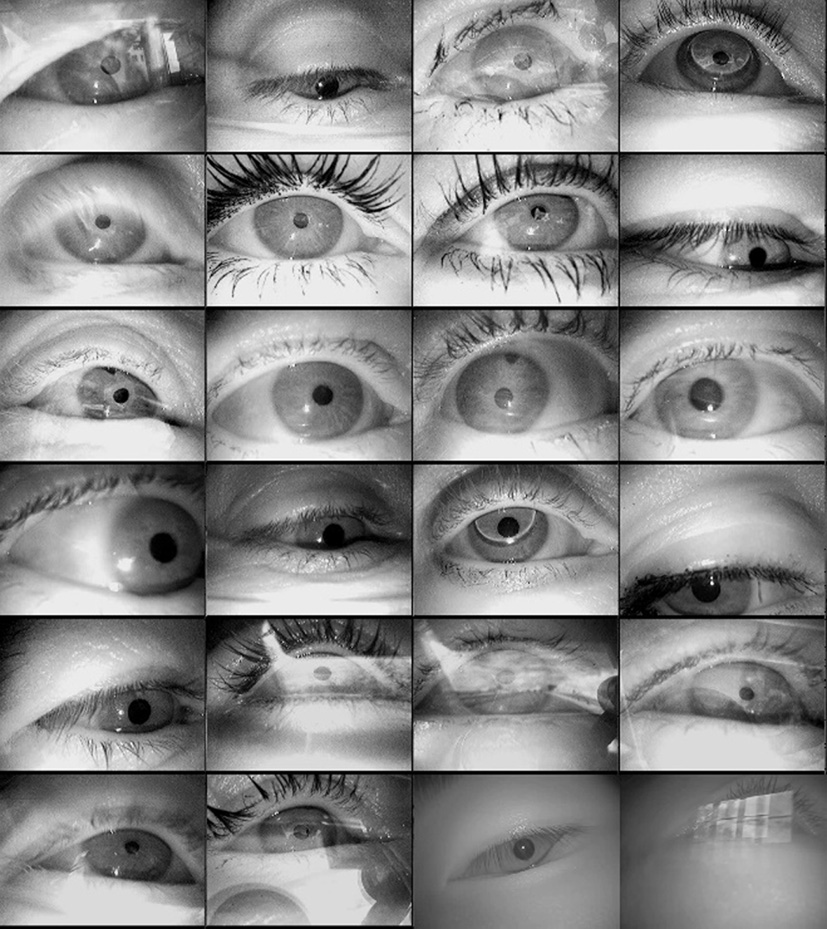

3.2 Ground truth generation

In order to obtain the coordinates of the pupil we are going to extract them as the center of a segmentation. A circular mask of size 20 pixels with value one was drawn in the position of the pupil’s center on a background of value zero, so that the DCNN generates a mask in which the pixels values represent the probability of being part of the circle centered in the pupil. Therefore, the network assigns high probability values to the pixels enclosed by the generated circle instead of providing the pupil’s coordinates directly. Figure 2 shows some examples of the ground truth masks for different input images.

Once the probability mask is obtained, we need to threshold it in order to obtain a binary image that classifies the pixels either as background or as belonging to the pupil circle. After this, further processing is needed to obtain the final coordinates of the pupil from this binary image. This is explained in detail in Section 3.5.

Figure 2.

Ground truth masks for different input images in which a circle of 20 pixels with ones was drawn in images of zero value.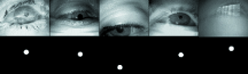

3.3 Network architecture

DCNN consist of several layers which contain neurons that perform local convolutions. The main variables of the model will be the weights of these convolutions. After a convolution, it is common to have an activation function such as a rectified linear unit (Relu), Sigmoid or hyperbolic tangent. The purpose of this activation function is to introduce non-linearity into the network, so that the network can learn a non-linear function.

After the initial convolutions and activation functions, a map of low-level features is obtained. In order to generate more informative features a common practice is to perform a pooling operation which consist in aggregating multiple low-level features over a small neighborhood. There are different ways to perform the pooling such as the max-pooling which simply reduces a neighborhood to its max value or the average-pooling which reduces it to the mean value. A pooling operation can be also performed using a convolution with stride. This adds more parameters to the model, but it allows learning a more complex feature combination. These are the basic components of a DCNN model. The model is finally trained using gradient descent optimization.

After this brief introduction to the DCNN, the following sections will describe the most important aspects of DeepEye architecture in more detail.

3.3.1 Batch Normalization and Batch Renormalization

Batch Normalization, [39] is a fundamental tool in Deep Learning that has been used over the last two years in several architectures. Batch Normalization helps to stabilize the distributions of internal activations during the training of the model, which makes the model less influenced by parameter initialization and enables the use of higher learning rates. These effects make the training more solid and faster. Batch normalization works on mini-batches in stochastic gradient training. It uses the mean and variance of the mini-batch to normalize it before the activation function, and also to estimate a moving average and variance that are used during inference. The drawback is that in order to obtain an accurate estimation for the mini-batch statistics, a sufficient number of examples in the mini-batch are needed, and these examples must be statistically independent. If the estimations in the mini-batches differ from the moving estimation, batch normalization will give poor results during inference.

The batch normalization was Tested in DeepEye. However, there were large differences between the performance of training and inference. This was probably due to the fact that the mini-batch used is small because of the size of our input images (384 $\times$ 288) and also because the images are very similar among them, so the independence of the mini-batch images was also in question.

In order to correct this problem, the creators of the Batch Normalization published an updated version called Batch Renormalization [40].

Batch Renormalization is an extension of batch normalization that solves the problem of having mini-batches with a small number of samples that are not independent. The aim of the batch renormalization is to reduce the dependence of model layer inputs on all the examples in the mini-batch and therefore the different activation between training and inference among the layers of the model. Batch renormalization ensures that the outputs computed by the model are dependent only on the individual examples and not on the entire mini-batch. At the same time, batch renormalization seems to retain the benefits of reducing the sensitivity to the initialization of the values in the kernels, while improving training speed compared to the traditional batch normalization. Based on all of these facts, batch renormalization was added to the model achieving lower differences between training and inference performance in comparison to the regular batch normalization.

3.3.2 Residual learning

The early works on modern deep learning showed that when you increase the number of layers of the network, i.e. the depth of the network, the error rate is reduced [26, 41, 42]. Nonetheless, when a certain point of depth is reached, the performance of the model starts to degrade rapidly [43, 44]; [25] shows that this degradation happens due to the difficulties of the solver to approximate identity maps by multiple non-linear layers. In order to address this problem, they propose residual learning, which consists on a shortcut that adds the input of a unit of several convolutions to its output. A schematic of the residual shortcut is shown in Fig. 3.

Consider a shallower architecture and its deeper counterpart that adds more layers onto it. If the shallower architecture is the optimal solution the following layers added in the deeper architecture should reproduce the identity and the error should be the same in both, whereas the degradation problem suggest that the solvers might have difficulties in approximating identity mappings by multiple non-linear layers. With the residual learning reformulation, if identity mappings are optimal, the solvers may simply drive the weights of the multiple non-linear layers towards zero in order to approach identity mappings. In real cases it is unlikely that identity mappings are optimal. However, the residual reformulation helps to precondition the problem if the optimal function is closer to an identity than to a zero mapping. In other words, the residual approach avoids the need of generating an identity function, which is hard to obtain, and instead just generate a nullity function which is easier to be generated by the convolution functions.

Figure 3.

Residual shortcut in a convolutional block.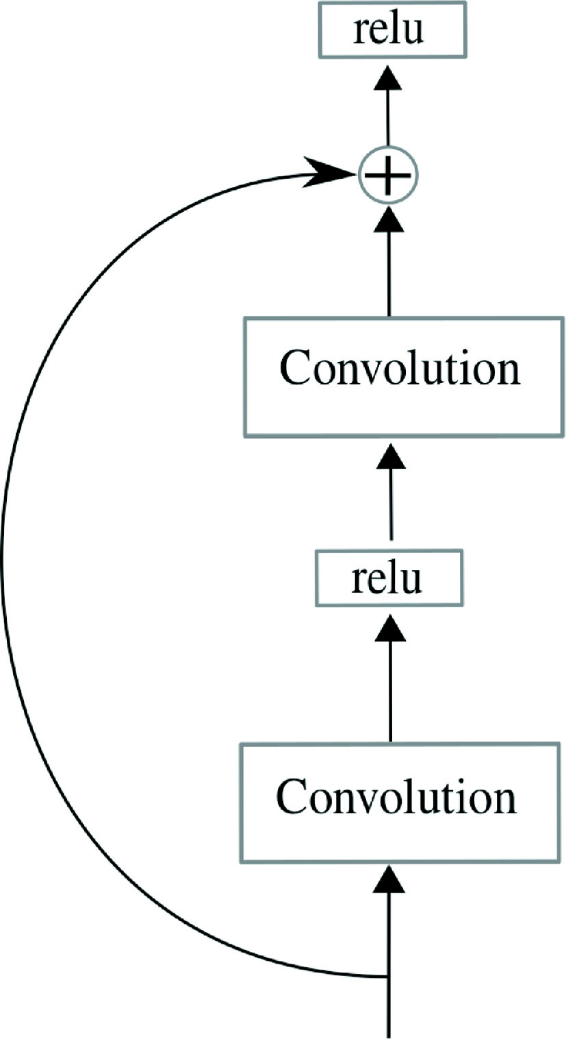

3.3.3 Atrous convolution

Atrous convolution was originally developed for the efficient computation of the undecimated wavelet transform in the “algorithme à trous” scheme [45]. This algorithm allows computing the responses of any layer at any desirable resolution. The atrous convolution for a two-dimensional signal can be defined as:

$\displaystyle{y}[{i}]=\sum\nolimits_{k}{x}[i+d\cdot k]{w}[{k}]$ (1)

where $i$ is the position in which the kernel $w$ is applied obtaining the value $y$ , $d$ corresponds to the stride that sample the input signal which is equivalent to convolving the input $x$ with a kernel that have $d-1$ zeros inserted between the kernel values. Figure 5 illustrates this. Atrous convolution has been used with successful results in the segmentation models proposed in [18, 30].

Figure 4.

Residual shortcut in a strided block.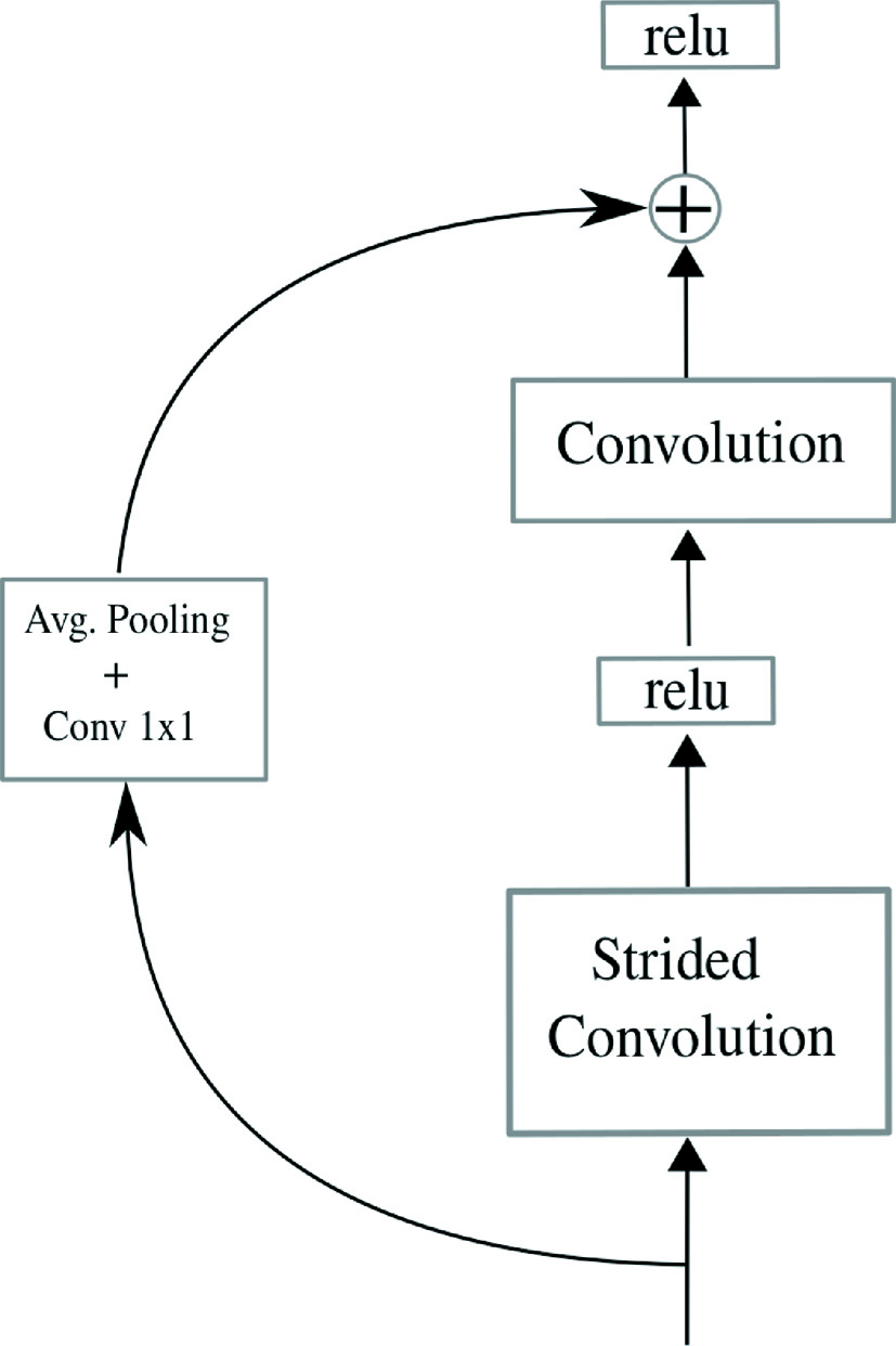

Atrous convolution allows enlarging the receptive field of the filters in the network. Therefore, it offers a good mechanism to control the field of view and finds the best combination of localization and context information. An example of this atrous kernels is shown in Fig. 5.

3.3.4 Atrous spatial pyramid pooling

Atrous Spatial Pyramid Pooling (ASPP) is inspired by the success of spatial pyramid pooling, [46, 47], which showed that it is effective to sample features at different scales for accurately and efficiently classifying regions of an arbitrary scale. This strategy has been used with great success in [18, 30] for image segmentation. Following these proposals, a similar version of their ASPP has been implemented.

The implemented ASPP consist in three 3 $\times$ 3 atrous blocks with different dilation rates (4, 8, 16), one 1 $\times$ 1 convolution and a max-pooling operation. The outputs of those operations are concatenated to perform a final 1 $\times$ 1 convolution to obtain the final logits, a schematic representation is showed in Fig. 6. It is important to notice that the atrous blocks have two identical atrous convolutions connected with a residual operation and in the max-pooling operation a zero padding is performed to maintain the same size.

Figure 5.

Examples of atrous 3 $\times$ 3 kernels with different rates. a) Atrous with $d=$ 1 produces the standard convolution. b) and c) Employ larger values of atrous rate that enlarge the model’s field-of-view enabling object encoding at multiple scales.

Figure 6.

Atrous spatial pyramid pooling used in deepeye.

Figure 7.

DeepEye schematic blocks.

3.3.5 Network overview

Figure 7 shows a schematic of DeepEye. The representation is composed of blocks that represent various convolutions and operations. The convolution blocks represent two convolutions with the residual operation. For details, see Fig. 3. The strided blocks perform a convolution with stride to reduce the dimension of the image followed by a convolution. It is important to notice that the residual must be reduced in dimensions and increased in number of channels when a strided block is performed. The dimension of the residual dimension is reduced using an average-pooling and the number of channels is increased performing a 1 $\times$ 1 convolution. Figure 4 shows a representation of the strided block. The ASPP blocks represent the pyramid operation of Fig. 6. It contains atrous blocks with different dilations that have two atrous convolution connected with the residual operation, a 1 $\times$ 1 convolution and a max-pooling operation. Finally, at the end of the network a bilinear interpolation is performed to increase 4 times the size of the output in order to obtain the same shape as the ground truth. The value $L$ represents the number of filters in the first convolution block and they are doubled after every strided block. In Section 4.1 the selection of the number of filters in the convolutions and the number of ASPP are discussed.

3.4 Training details

The training was performed using cross-entropy and soft-max. RMSprop with a learning rate of 10–3 and a decay of 0.9 was used as optimization method. One of the main difficulties with the data sets is the unbalance in the number of images across them, due to some data sets containing more than 10.000 images while others contain less than 1.000. Therefore, to avoid over fitting to the large data sets, every data set was repeated as many times as needed to have the same number of images in every data set. Data augmentation was also performed by randomly rotating between 0 and 360 degrees every image. This was done with the aim of making the network more robust to different camera-to-eye positions. The mini-batch size used in the following experiments is 4 and it contains random images coming from any data set in the training set. The minibatch size can be larger and the results are the same. We chose a size of 4 as it was the maximum mini-batch value for the biggest architecture tested. The models take around 60.000 iterations to converge.

3.5 Post-processing

As explained in Section 3.2 the network output is a probability image in which the pixel value represents the probability of being part of the circle centered in the pupil. The aim of this post-processing is to compute the coordinates of the pupil from this probability mask. First, the probability mask needs to be thresholded to obtain a binary image. Then, the biggest blob is extracted and the coordinates of its center will be considered the final pupil coordinates. An iterative thresholding has been implemented to account for images where the network has low confidence, which happens when the pupil is occluded or has low contrast.

The procedure consists of the following steps:

•
A threshold ${t}$ is applied to the mask.
•
A blob detector is applied to locate the biggest blob.
•
If the blob is not larger than $P$ pixels, the threshold ${t}$ is reduced by ${tn}={tn}-{1}-{r}$ and we proceed again from step 1.
•
If the blob is larger than ${P}$ , its center is computed and reported as pupil center.

The parameters values selected were ${t}$ $=$ 0.5 as starting threshold, ${r}$ $=$ 0.05 for reducing the threshold and ${P}$ $=$ 100 as the minimum number of pixels in the blob.
4. Evaluation

In order to implement DeepEye, Tensorflow was used to build the deep learning network and OpenCV was used for the image processing. The algorithm has been tested in a PC with a Nvidia Tesla K40 and a Intel i7-6700K. The results have been reported in terms of the average pupil detection rate as a function of pixel distance between the coordinates obtained from DeepEye and the hand-labeled coordinates. For comparison with other methods, the percentage of frames with an error lower than 5 pixels have been reported, in a similar way to previous techniques [17, 19, 24].

4.1 Model selection

In this section the testing of several architectures with a different number of filters and ASPP blocks is reported. The first 50% of the frames of every data set were used as training set and the remaining 50% were used for testing. A combination of architectures using 2, 3 or 4 ASPP blocks and 8, 16, 32 or 64 filters was trained and tested. Figure 8 depicts the results as the percentage of frames in which the pupil is detected with a distance error lower than 5 pixels.

Figure 8.

Detection rate with an error lower than 5 pixels for the architectures evaluated. The network architectures tested are encoded in DXLY, being X the number of ASPP used and Y the number of filters in the initial layer.

Figure 9.

Frames per second and number of trainable parameters with every architecture evaluated. The network architectures tested are encoded in DXLY, being X the number of ASPP used and Y the number of filters in the initial layer.

Figure 10.

(a) Input images, (b) Probability masks, (c) Thresholded mask, (d) Masks with the center of the blob and (e) Final center of the pupil.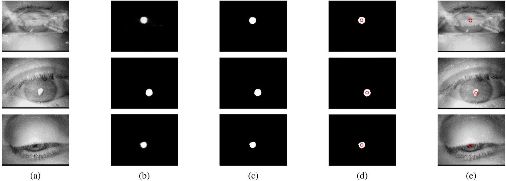

The architectures tested perform slightly different. Increasing the number of layers tends to improve the results until a certain number of layers is reached, a point at which figures decrease slightly. Something similar happens with the number of ASPP. The performance is increased until the 4th ASPP is added. The difference in performance can be due to over-fitting because the network is using too many trainable parameters to solve the problem. Nonetheless, the differences in performance are less than 3%. Figure 9 depicts the number of trainable parameters used in the tested architectures.

We have also evaluated the frames per second (fps) that the network can process in our set-up. These results are shown in Fig. 9. As the number of parameters is increased, the processing speed of the architectures decreases from 53 fps (19 ms per frame) to 4 fps (250 ms per frame). The post-processing steps take 2 ms in average, so the processing bottleneck is in the neural network.

Taking into account these results, the architecture with 2 ASPP blocks and 16 filters was selected as its performance is almost the same as that of a 3 block and 32 filter architectures, achieving speeds higher than 30 fps. In comparison with other algorithm of the state of art our network is very slow taking into account that ElSe and ExCuSe can process around 150 fps, depending on the hardware used, but our intention is mainly for off-line applications in which a high frame-rate processing and high precision is needed.

Table 1

Quantitative results of the segmentation

Accuracy	Sensitivity	Specificity	Kappa-factor
0.921	0.896	0.999	0.905

4.2 Segmentation results

Despite the fact that the segmentation is not the aim of this proposal, it is interesting in order to have an intuition of how our method is working. Figure 10 shows some examples of the probability maps provided by the network, the result after applying the threshold and finally the center founded by the blob analysis. Table 1 shows the Accuracy, Sensitivity, Specificity and Kappa factor of the segmentation compared to the generated ground truth. In all these figures the network composed by 2 ASPP and 16 initial filters was used.

4.3 Cross validation

The model with 2 ASPP blocks (depth $=$ 2) and 16 initial filters ( $L=$ 16) was used for the final evaluation. In this section every data set was tested and the results have been compared with ElSe [17], ExCuse [19] and Swirski [14] which was shown to provide the best results before our work in the data sets used.

In order to do a fair comparison a cross validation between the data sets has been performed. This cross validation is performed using all the samples from a certain data set as testing set and using all the remaining data sets as training set. This provides information about the capability of generalization of DeepEye.

Figure 11.

Detection error in function of the pixel distance in the cross validation compared with ElSe, ExCuSe and Swirski.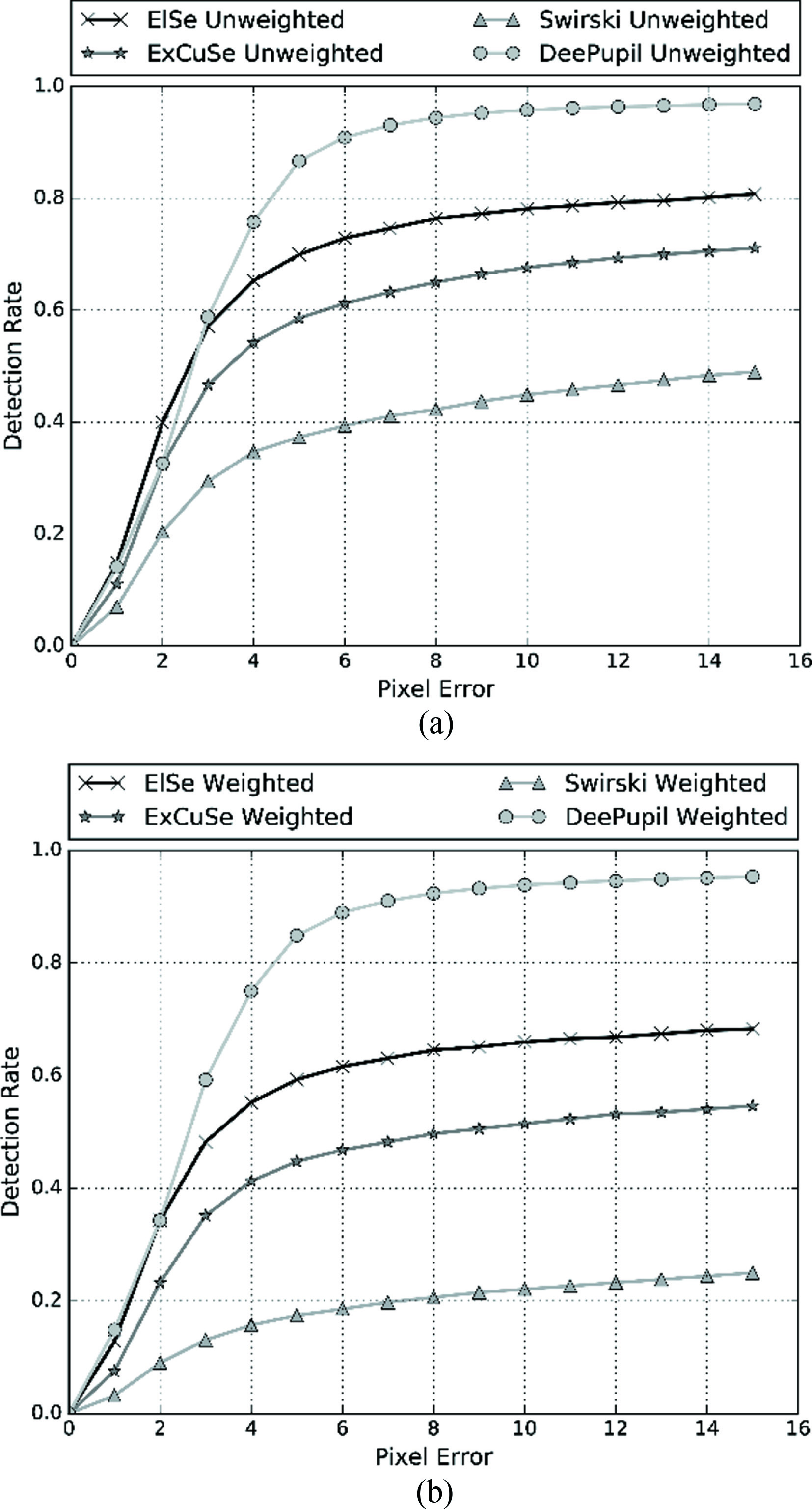

Table 2

Performance comparison among data sets between Swirski, ExCuSe, ElSe and DeepEye in terms of detection rate up to an error of 5 pixels

	Swirski	ExCuSe	ElSe	DeepEye
I	5.11	70.95	85.52	86.40
II	26.34	34.26	65.35	82.97
III	6.81	39.44	63.60	93.18
IV	34.54	81.58	83.24	92.99
V	77.85	77.28	84.87	96.95
VI	19.34	53.18	77.52	92.93
VII	39.35	46.91	59.51	84.27
VIII	41.90	56.83	68.41	86.50
IX	24.09	74.608	86.72	91.91
X	29.88	79.76	78.93	92.38
XI	20.31	56.49	75.27	94.19
XII	71.37	79.20	79.39	85.30
XIII	61.51	70.26	73.52	78.81
XIV	53.30	57.57	84.22	95.73
XV	60.88	52.34	57.30	89.16
XVI	17.86	49.49	59.95	82.39
XVII	70.90	77.99	89.55	94.89
XVIII	12.39	22.24	50.86	73.72
XIX	9.03	26.45	33.04	77.92
XX	17.93	52.37	67.90	92.04
XXI	8.09	43.54	41.47	88.42
XXII	1.98	27.93	48.98	80.13
XXIII	96.54	93.86	94.34	96.22
XXIV	44.43	45.21	52.97	54.61

Figure 11 depicts the performance in terms of the detection rate achieved with less than a certain pixel distance between the output and the hand labeled ground truth. Two results are displayed: the weighted result is the percentage of correctly detected pupil centers for all images in all data sets and the unweighted result is the mean of the results among all data sets not accounting for the differences in data set sizes.

Table 2 presents the performance of DeepEye for every data set compared with ElSe, ExCuSe and Swirski. The metric used is the percentage of frames in which the pupil is detected with a distance error lower than 5 pixels. DeepEye outperforms ElSe by 26% and it also shows much more consistency, as the detection rate is higher than 70% in most data sets. DeepEye achieves an 87% detection rate with less than 5 pixels of error in contrast to the rate of 69% achieved by ElSe. DeepEye also achieves a 96% detection rate with less than 10 pixels of error, this result indicates that the pupil is detected in most of the frames whereas in some cases the center cannot be localized precisely.

5. Input size

DCNN are usually trained with images with the same size in order to maintain a homogeneous scale for the features. This is due to the fact that training with different size is not always possible with the architecture used or makes the training harder. Some approaches are trying to solve these problems using different models for the different resolutions [48]. Nonetheless these approaches increase the complexity of the models. DeepEye was trained with images with a fixed size of 384 $\times$ 288, which is the size of the images in the data set collection. Therefore, if images with different size are used as input, the performance will be reduced significantly. One solution could be resizing the input images, processing them and transform the coordinates to the original size of the images at the end of the pipeline. This approach reduces the precision of the final coordinates. If instead of transforming the coordinates, the probability mask is resized to the original size before applying the thresholding step, the final coordinates obtained are more accurate.

6. Conclusions

Eye tracking is a very useful technology for several applications, and there is a growing need for robust and efficient algorithms. We have presented DeepEye, an eye-tracking technique based on deep learning that outperforms the state of the art in eye-tracking algorithms, achieving high accuracy and consistency. The network is based on atrous convolutions in a ASPP scheme that generates a segmentation of the pupil. We compared DeepEye to the state of the art techniques for pupil tracking, obtaining an 87% of frames with less than 5 pixel error. DeepEye can process sequences at 32 fps with a Tesla K40 Graphical Processing Unit, and 25 fps with a Nvidia GTX 1060 which is suitable for a real time scenario. DeepEye was specially designed for outdoor scenarios and the authors highly encourage to use it in experiments in which a high accuracy of the pupil detection is needed, such as detection of saccades for neurological diseases.

As future work, we will optimize the architecture and reduce its complexity in order to work in lighter or embedded hardware. To achieve this aim, the use of binary networks [49] that reduce the complexity of the computation using just binary values for the kernels could be a solution. Also, reducing the image size and the number of parameters in the network, or the use of schemes such as R-CNN to make a full convolutional algorithm will be another asset to introduce in a future version of DeepEye.

Footnotes

Acknowledgments

This work was partially funded by project DPI2015-68664-C4-1-R of the Spanish Ministry of Economy and by Banco de Santander and Universidad Rey Juan Carlos Funding Program for Excellence Research Groups ref. “Computer Vision and Image Processing (CVIP)”. We gratefully acknowledge the support of NVIDIA Corporation with the donation of the Nvidia Tesla K40 GPU used for this research, and the anonymous reviewers that helped to improve the paper with their comments.

References

Deng

Hsu

Lin

Tuan

Chang

. EOG-based human-computer interface system development. Expert Systems with Applications. 2010; 37(4): 3337-3343.

Cannan

. Human-machine interaction (HMI): A survey. University of Essex. 2011.

Anderson

MacAskill

. Eye movements in patients with neurodegenerative disorders. Nature Reviews Neurology. 2013; 9(2): 74-85.

Dowiasch

Backasch

Einhäuser

Leube

Kircher

Bremmer

. Eye movements of patients with schizophrenia in a natural environment. European Archives of Psychiatry and Clinical Neuroscience. 2016; 266(1): 43-54.

Xia

Zhang

Wang

Liu

, et al. Eye movement indices in the study of depressive disorder. Shanghai Archives of Psychiatry. 2016; 28(6): 326-335.

Yang

. Real-time eye, gaze, and face pose tracking for monitoring driver vigilance. Real-Time Imaging. 2002; 8(5): 357-377.

Wang

Yang

Ren

Zheng

. Driver fatigue detection: A survey. In: Intelligent Control and Automation, 2006. WCICA 2006. The Sixth World Congress on IEEE. 2006; 2: 8587-8591.

Krugman

Fox

Fletcher

Fischer

Rojas

. Do adolescents attend to warnings in cigarette advertising? An eye-tracking approach. Journal of Advertising Research. 1994; 34: 39-39.

Resnick

Albert

. The impact of advertising location and user task on the emergence of banner ad blindness: An eyetracking study. International Journal of Human-Computer Interaction. 2014; 30(3): 206-219.

10.

Mosimann

Müri

Burn

Felblinger

O’brien

McKeith

. Saccadic eye movement changes in Parkinson’s disease dementia and dementia with Lewy bodies. Brain. 2005; 128(6): 1267-1276.

11.

Bittencourt

Velasques

Teixeira

Basile

Salles

Nardi

, et al. Saccadic eye movement applications for psychiatric disorders. Neuropsychiatric Disease and Treatment. 2013; 9: 1393.

12.

Goni

Echeto

Villanueva

Cabeza

. Robust algorithm for pupil-glint vector detection in a video-oculography eyetracking system. In: Pattern Recognition, 2004. ICPR 2004. Proceedings of the 17th International Conference on 4 IEEE. 2004; 4: 941-944.

13.

Long

Tonguz

Kiderman

. A high speed eye tracking system with robust pupil center estimation algorithm. In: Engineering in Medicine and Biology Society, 2007. EMBS 2007. 29th Annual International Conference of the IEEE. 2007; 3331-3334.

14.

Swirski

Bulling

Dodgson

. Robust real-time pupil tracking in highly off-axis images. In: Proceedings of the Symposium on Eye Tracking Research and Applications. ACM. 2012; 173-176.

15.

Valenti

Gevers

. Accurate eye center location through invariant isocentric patterns. IEEE Transactions on Pattern Analysis and Machine Intelligence. 2012; 34(9): 1785-1798.

16.

Schnipke

Todd

. Trials and tribulations of using an eye-tracking system. In: CHI’00 Extended Abstracts on Human Factors in Computing Systems. ACM. 2000; 273-274.

17.

Fuhl

Santini

Kübler

Kasneci

. Else: Ellipse selection for robust pupil detection in real-world environments. In: Proceedings of the Ninth Biennial ACM Symposium on Eye Tracking Research & Applications. ACM. 2016; 123-130.

18.

Chen

Papandreou

Schroff

Adam

. Rethinking atrous convolution for semantic image segmentation. arXiv preprint arXiv170605587. 2017.

19.

Fuhl

Kübler

Sippel

Rosenstiel

Kasneci

. Excuse: Robust pupil detection in real-world scenarios. In: International Conference on Computer Analysis of Images and Patterns. Springer. 2015; 39-51.

20.

Keil

Albuquerque

Berger

Magnor

. Real-time gaze tracking with a consumer-grade video camera. 2010.

21.

Zhu

Moore

Raphan

. Robust pupil center detection using a curvature algorithm. Computer Methods and Programs in Biomedicine. 1999; 59(3): 145-157.

22.

Winfield

Parkhurst

. Starburst: A hybrid algorithm for video-based eye tracking combining feature-based and model-based approaches. In: Computer Vision and Pattern Recognition-Workshops, 2005. CVPR Workshops. IEEE Computer Society Conference on IEEE. 2005. 79-79.

23.

Javadi

Hakimi

Barati

Walsh

Tcheang

. SET: a pupil detection method using sinusoidal approximation. Frontiers in Neuroengineering. 2015; 8.

24.

Fuhl

Santini

Kasneci

. PupilNet: Convolutional neural networks for robust pupil detection. arXiv preprint arXiv160104902. 2016.

25.

Zhang

Ren

Sun

. Deep residual learning for image recognition. In: The IEEE Conference on Computer Vision and Pattern Recognition (CVPR). 2016.

26.

Szegedy

Liu

Jia

Sermanet

Reed

Anguelov

, et al. Going deeper with convolutions. In: The IEEE Conference on Computer Vision and Pattern Recognition (CVPR). 2015.

27.

Badrinarayanan

Kendall

Cipolla

. Segnet: A deep convolutional encoder-decoder architecture for image segmentation. arXiv preprint arXiv151100561. 2015.

28.

Noh

Hong

Han

. Learning deconvolution network for semantic segmentation. In: The IEEE International Conference on Computer Vision (ICCV). 2015.

29.

Ronneberger

Fischer

Brox

. U-net: Convolutional networks for biomedical image segmentation. In: International Conference on Medical Image Computing and ComputerAssisted Intervention. Springer. 2015; 234-241.

30.

Chen

Papandreou

Kokkinos

Murphy

Yuille

. Deeplab: Semantic image segmentation with deep convolutional nets, atrous convolution, and fully connected crfs. arXiv preprint arXiv160600915. 2016.

31.

Redmon

Divvala

Girshick

Farhadi

. You only look once: Unified, real-time object detection. In: Proceedings of the IEEE Conference on Computer Vision and Pattern Recognition. 2016; 779-788.

32.

Wang

Shrivastava

Gupta

. A-fast-rcnn: Hard positive generation via adversary for object detection. arXiv preprint arXiv170403414. 2017; 2.

33.

Gkioxari

Dollár

Girshick

. Mask r-cnn. In: Computer Vision (ICCV), 2017 IEEE International Conference on IEEE. 2017; 2980-2988.

34.

Lin

Nie

. Structural damage detection with automatic feature-extraction through deep learning. Computer-Aided Civil and Infrastructure Engineering. 2017; 32(12): 1025-1046.

35.

Zhang

Wang

Yang

Dai

Peng

, et al. Automated pixel-level Pavement crack detection on 3D asphalt surfaces using a deep-learning network. Computer-Aided Civil and Infrastructure Engineering. 2017; 32(10): 805-819.

36.

Acharya

Hagiwara

Tan

Adeli

. Deep convolutional neural network for the automated detection and diagnosis of seizure using EEG signals. Computers in Biology and Medicine. 2017.

37.

Rafiei

Adeli

. A novel machine learning model for estimation of sale prices of real estate units. Journal of Construction Engineering and Management. 2015; 142(2): 04015066.

38.

Kasneci

Sippel

Aehling

Heister

Rosenstiel

Schiefer

, et al. Driving with binocular visual field loss? A study on a supervised on-road parcours with simultaneous eye and head tracking. PloS One. 2014; 9(2): e87470.

39.

Ioffe

Szegedy

. Batch normalization: Accelerating deep network training by reducing internal covariate shift. In: International Conference on Machine Learning. 2015; 448-456.

40.

Ioffe

. Batch renormalization: Towards reducing minibatch dependence in batch-normalized models. arXiv preprint arXiv170203275. 2017.

41.

Krizhevsky

Sutskever

Hinton

. Imagenet classification with deep convolutional neural networks. In: Advances in Neural Information Processing Systems. 2012; 1097-1105.

42.

Simonyan

Zisserman

. Very deep convolutional networks for large-scale image recognition. arXiv preprint arXiv14091556. 2014.

43.

Sun

. Convolutional neural networks at constrained time cost. In: Proceedings of the IEEE Conference on Computer Vision and Pattern Recognition. 2015; 5353-5360.

44.

Srivastava

Greff

Schmidhuber

. Highway networks. arXiv preprint arXiv150500387. 2015.

45.

Holschneider

Kronland-Martinet

Morlet

Tchamitchian

. A real-time algorithm for signal analysis with the help of the wavelet transform. In: Wavelets. Springer. 1990; 286-297.

46.

Lazebnik

Schmid

Ponce

. Beyond bags of features: Spatial pyramid matching for recognizing natural scene categories. In: Computer Vision and Pattern Recognition, 2006 IEEE Computer Society Conference on IEEE. 2006; 2: 2169-2178.

47.

Zhang

Ren

Sun

. Spatial pyramid pooling in deep convolutional networks for visual recognition. In: European Conference on Computer Vision. Springer. 2014; 346-361.

48.

van Noord

Postma

. Learning scale-variant and scaleinvariant features for deep image classification. Pattern Recognition. 2017; 61: 583-592.

49.

Courbariaux

Bengio

David

. Binaryconnect: Training deep neural networks with binary weights during propagations. In: Advances in Neural Information Processing Systems. 2015; 3123-3131.