Unilateral sensorineural hearing loss identification based on double-density dual-tree complex wavelet transform and multinomial logistic regression

Abstract

AIM:

Unilateral sensorineural hearing loss is a brain disease, which causes slight morphology changes within brain structure. Traditional manual method may ignore this change.

METHOD:

In this work, we developed a novel method, based on the double-density dual-tree complex (DDDTCWT), and radial basis function kernel principal component analysis (RKPCA) and multinomial logistic regression (MLR) for the magnetic resonance imaging scanning. We first used DDDTCWT to extract features. Afterwards, we used RKPCA to reduce feature dimensionalities. Finally, MLR was employed to be the classifier.

RESULT:

The 10 times of 10-fold stratified cross validation showed our method achieved an overall accuracy of 96.44 $\pm$ 0.88%. The sensitivities of detecting left-sided sensorineural hearing loss, right-sided sensorineural hearing loss, and healthy controls were 96.67 $\pm$ 2.72%, 96.67 $\pm$ 3.51%, and 96.00 $\pm$ 4.10%, respectively.

CONCLUSION:

Our method performed better than both raw and improved AlexNet, and eight state-of-the-art methods via a stringent statistical 10 $\times$ 10-fold stratified cross validation. The MLR gives better classification performance than decision tree, support vector machine, and back-propagation neural network.

Keywords

Unilateral sensorineural hearing loss dual-tree complex wavelet transform kernel principal component analysis multinomial logistic regression double-density dual-tree complex wavelet transform magnetic resonance imaging alexNet

1. Introduction

Hearing loss is a partial or dead inability to hear. It may be caused by a massive of different problems, such as birth complication [1], infection [2], medications [3], ageing [4], genetics, noise [5], trauma [6], toxins [7], etc. The hearing loss is defined when the subject cannot hear 25 decibels and above for more than one year. Disabling hearing loss is defined as hearing loss greater than 40 decibels (dB) in the better hearing ear in adults and a hearing loss greater than 30 dB in the better hearing ear in children. Until 2017, it is reported by word health organization (WHO) that there are about 466 million people suffering from disabling hearing loss, and 34 million of these are kids. According to the estimation made by WHO, there will be over 900 million people have disabling hearing loss by 2050. 60% of childhood hearing loss is caused by preventable causes. The unaddressed hearing loss caused an annual global cost of 750 billion dollars every year. Interventions to prevent, identity and address hearing loss are cost effective and can bring great benefits to individuals. Therefore, in this paper, we proposed using machine learning method for the early detection of one specific type of hearing loss, which can be effectively visually inspected from Magnetic resonance imaging (MRI).

Sensorineural hearing loss is a type of hearing loss. Its cause may lie in either sensory tissues or neural tissues [8]. It may occur in one or both ears. In this study, we aim to detect unilateral sensorineural hearing loss (USHL) into two types: left-sided and right-sided.

MRI is an efficient tool to help diagnose USHL, because the USHL patients have distinct difference with healthy controls from the view of brain structures [9]. Nevertheless, these differences are slight and subtle especially in the prodromal stage in USHL disease. Therefore, computer vision techniques are essential to help neuro-radiologist to find those minor alterations.

In the last decade, Li [10] used fractional Fourier transform (FRFT) to detect left-sided and right-sided hearing loss. Chen [11] used wavelet packet decomposition (WPD) technique and least-square support vector machine (LSSVM). Gorriz and Ramírez [12] combined wavelet entropy (WE) and directed acyclic graph support vector machine (DAG-SVM). Chen Y. and Chen X.-Q. [13] employed three successful techniques: discrete wavelet transform (DWT), principal component analysis (PCA), and generalized eigenvalue proximal support vector machine (GEPSVM). Sun [14] employed wavelet energy, and proposed a quantum-behaved particle swarm optimization method. Wu [15] used contrast-limited adaptive histogram equ- alization approach. Lu [16] used radial basis function neural network. Chen [17] used fractal dimension based on Minkowski-Bouligand method to detect pathological brains. Lu [18] used wavelet packet entropy and back propagation (BP) algorithm. Pereira [19] used a Hu moment invariant (HMI) approach. Jia [20] used a deep autoencoder method.

After studying above literatures, we found they share three common problems: (i) Their datasets are imbalanced. This is because healthy controls are easily enrolled, while hearing loss patients are usually with other brain diseases, and hence those patients are not obedient for MRI scanning. (ii) They used wavelet or its variant as the feature, but wavelet decomposition can only detect textures along horizontal, vertical and diagonal directions. (iii) The performance of these detector systems are not satisfying and can be improved.

To solve these issues, Wang et al. [21], our previous work in IWINAC 2017, enrolled more USHL patients to balance the dataset. Besides, they proposed to combine dual-tree complex wavelet transform (DTCWT) and kernel principal component analysis to reduce the features. They chose the multinomial logistic regression as the classifier.

This paper is an extension of Wang et al. [21]. The new extensions include following eleven points: (i) We increase the 60-subject dataset to 90-subject. (ii) We replace dual-tree complex wavelet transform (DTCWT) with double-density DTCWT (DTCWT). (iii) We add contents describing discrete wavelet transform, double-density DTCWT, principal component analysis. (iv) We add three simulation experiments. (v) We add an experiment to illustrate the decomposition result by double-density DTCWT. (vi) We add an experiment to show the statistical analysis of our method. (vii) We design an experiment to select the optimal feature extraction method and find the optimal decomposition level. (viii) We design an experiment to select the optimal feature reduction method and corresponding optimal thresholding. (ix) We compare proposed MLR to traditional classifier (decision tree, support vector machine, and back-propagation neural network). (x) We compare our proposed method to a pretrained deep learning method (AlexNet). (xi) We use GPU to accelerate our method and compared GPU with CPU in terms of computation time.

The structure of this paper is organized as follows: Section 2 contains the demographics of 90 subjects. Section 3 shows the image preprocessing method. Section 4 describes three feature extraction methods: discrete wavelet transform (WT), dual-tree complex wavelet transform (DTCWT), and double-density DTCWT. Section 5 relates three dimensionality reduction methods: principal component analysis (PCA), and two kernel PCA methods. Section 6 presents the fundamental of multinomial logistic regression, and the implementation of our whole method. Section 7 offers the results of three simulation experiments. Section 8 gives the results over realistic data. Finally, Section 9 provides the conclusion of this paper.

2. Subjects

This study followed to use the 60 subjects in our previous work [21], and we enrolled 30 new subjects. Finally, we have a 90-subject dataset, including 30 healthy controls (HC), 30 left-sided sensorineural hearing loss (LSHL) patients, and 30 right-sided sensorineural hearing loss (RSHL) patients. The demographic data of the balanced new dataset is listed in Table 1, which clearly shows that all three classes are well matched with regards to gender, age, and education level.

The inclusion and exclusion criteria, the pure tone audiometry implementation, the imaging parameters are all the same as in Reference [13]. Ethics Committee of Southeast University approved this research. The audiograms of two patients are shown in Fig. 1.

Table 1
Demographics of the 90-subject dataset

	LSHL	RSHL	HC
Number	30	30	30
Age (year)	51.6 $\pm$ 9.6	53.4 $\pm$ 7.9	53.8 $\pm$ 6.1
Gender (m/f)	14/16	13/17	14/16
Education level (year)	12.2 $\pm$ 2.1	12.4 $\pm$ 2.3	11.9 $\pm$ 2.8
Disease duration (year)	17.9 $\pm$ 17.1	16.5 $\pm$ 16.3	–
PTA of left ear (dB)	79.1 $\pm$ 15.8	23.4 $\pm$ 4.0	21.9 $\pm$ 2.1
PTA of right ear (dB)	21.5 $\pm$ 3.7	80.5 $\pm$ 19.4	21.2 $\pm$ 2.0

Data are mean $\pm$ SD, PTA $=$ pure tone average, m $=$ male, f $=$ female.

Figure 1.

PTA scores of two subjects.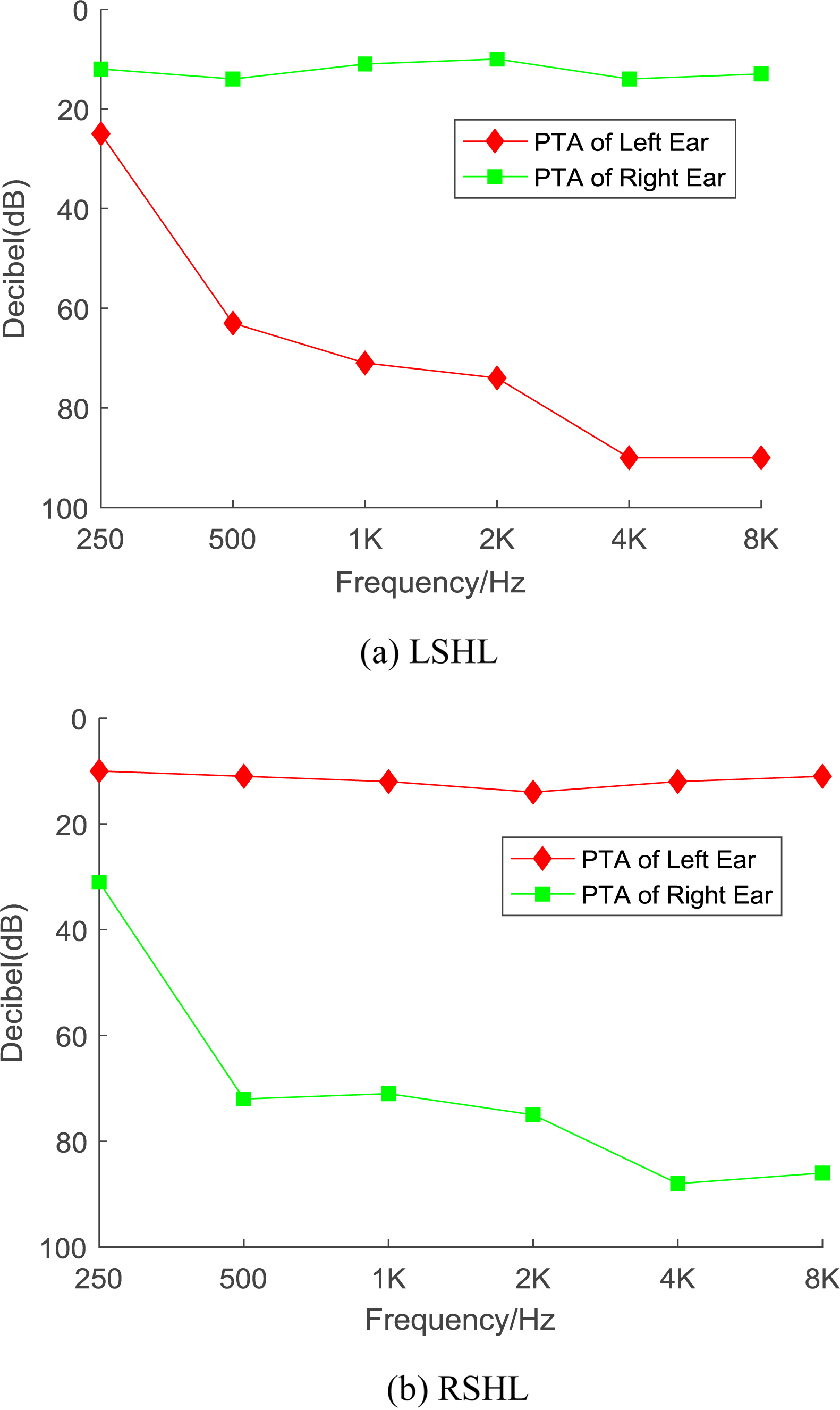

Figure 2.

Illustration of detected case of left hearing loss, right hearing loss and healthy case.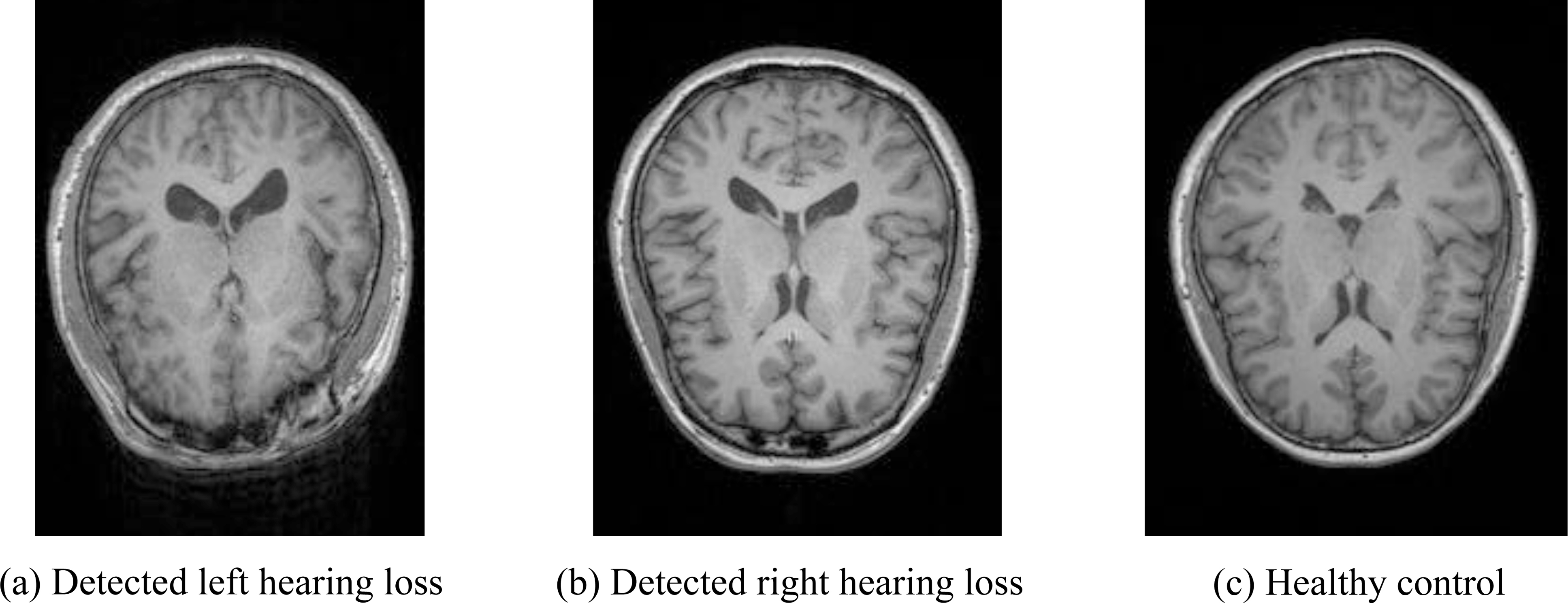

The images were obtained via a Siemens Verio Tim 3.0 T MR scanner (Siemens Medical Solutions, Erlangen, Germany). The parameters for imaging were set as Time of Echo (TE) $=$ 2.48 ms, Time of Repetition (TR) $=$ 1900 ms, Time of Inversion (TI) $=$ 900 ms, Flip Angle (FA) $=$ 9 ${}^{\circ}$ , Field of View (FOV) $=$ 256 mm $\times$ 256 mm, matrix $=$ 256 $\times$ 256, slice thickness $=$ 1 mm. All the subjects are required to lie still and eyes closed but not fall asleep. Via the MP_RAGE sequence, we can get 176 sagittal slices for the whole brain. Figure 2 shows an example of left hearing loss, right hearing loss and healthy case.

3. Image preprocessing

Image preprocessing follows the standard steps. First, the brain extraction tool (BET) v2.1 software [22] was employed to extract brain tissues. Figure 3a shows an original head image. Figure 3b gives the BET result, where the yellow line marks the brain area. Figure 3c shows the final extracted brain image.

Second, all the brain images of 90 subjects were normalized to the Montreal neurologic institute (abbreviated as MNI) template by FMRIB’s Linear Image Registration Tool (FLIRT) [23, 24] and FMRIB’s Nonlinear Image Registration Tool (FNIRT) [25]. Third, we resampled them to 2 mm isotropic voxels, and smoothed them by Gaussian kernel. Finally, three experienced otologists were instructed to select the optimal slice for each subject that covers his/her majority tissues related to hearing. The selected slice was at $Z=$ 88 (i.e., 16 mm) in MNI coordinate space.

Figure 3.

Brain extraction result (the yellow line marks the brain region).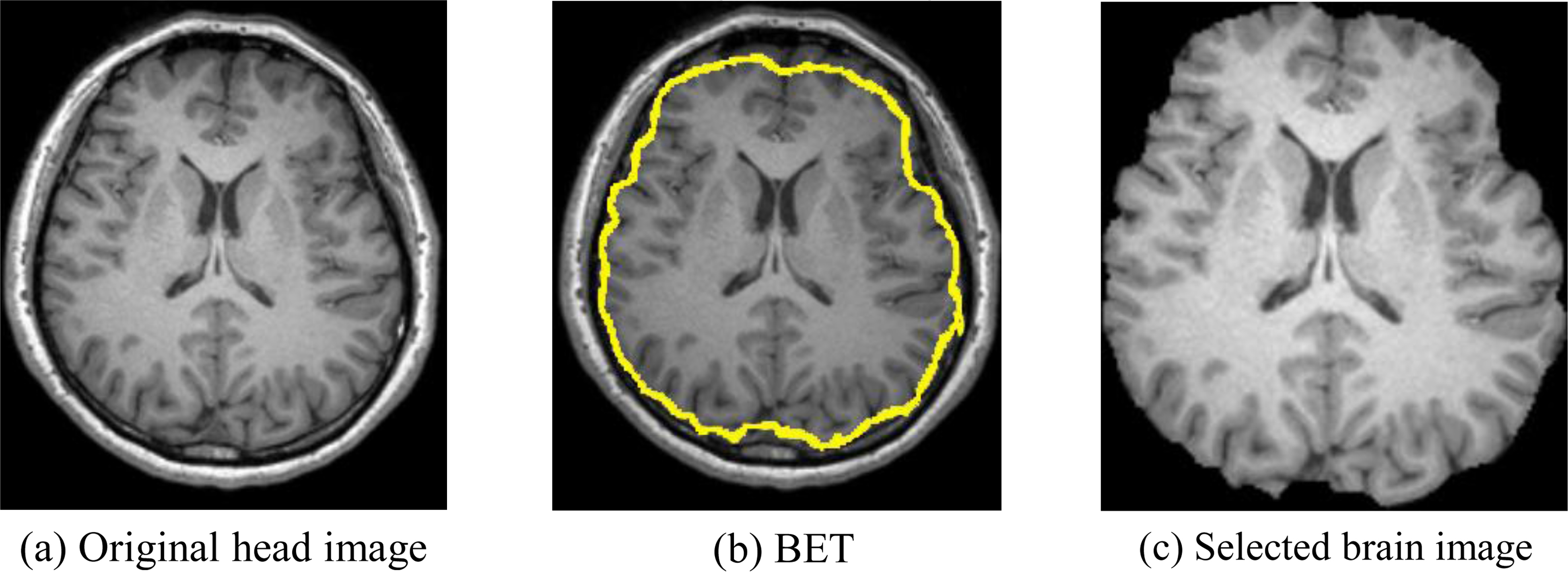

Here we select the slice at $Z=$ 88 by experience of radiologists. In the experiment, we shall design an exhaustive search method, in which we extract different slices from $Z=$ 30 ( $-$ 42 mm) to $Z=$ 150 (78 mm) with increase of 1. These slices are shown in Fig. 4. Here the gap is every 10 slices for clear view.

Figure 4.

Illustration of potential selected slices.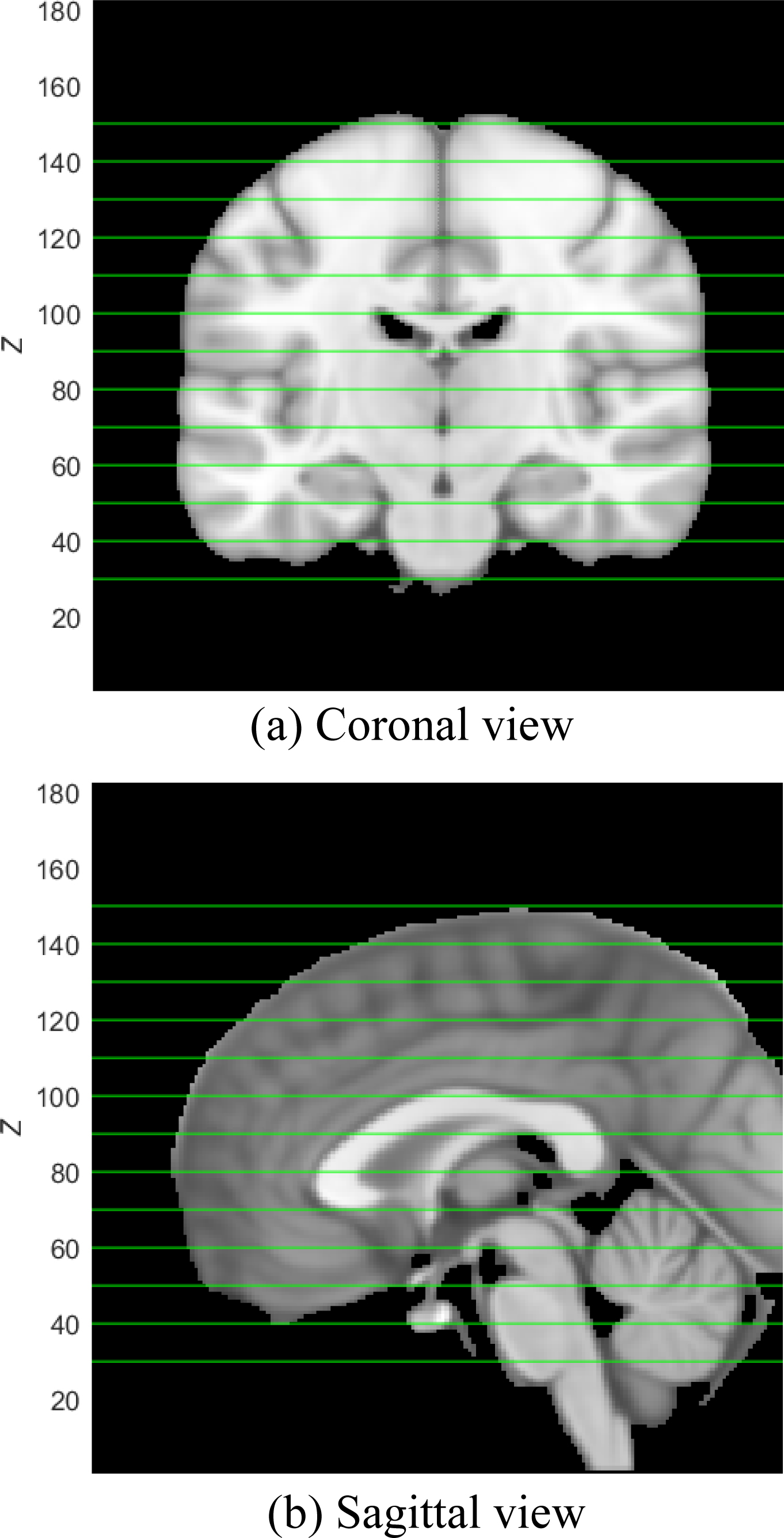

4. Feature extraction

The physical structures of the brain are similar to fingerprints as they both have gyrus, which can be analyzed by wavelet successfully. Hence, in this paper, we proposed to use wavelet for the brain structure analysis. In this Section, we briefly introduced three wavelet transforms: discrete wavelet transforms, dual-tree complex wavelet transforms, and double-density dual-tree complex wavelet transform.

4.1 Discrete wavelet transform

The discrete wavelet transform is a mathematical implementation of wavelet transform [26, 27] using discrete sets of various scales and translations. Assume $I$ represent a given time-domain signal, $k$ represents the sampling point with equal time interval, $h$ and $g$ represent a high-pass filter and low-pass filter, respectively,

$\displaystyle D(k)=\sum_{m}{h(2k-m)\times I(m)}$ (1) $\displaystyle A(k)=\sum_{m}{g(2k-m)\times I(m)}$ (2)

where $D$ and $A$ represents the detail and approximation coefficient sub-bands

When $I$ is extended to be a 2D image, we have four new sub-bands [28, 29]. The horizontal $H$ sub-band is obtained by passing image $I$ through a high-pass filter along $x$ -axis and low-pass filter along $y$ -axis. The vertical $V$ subband is obtained by passing the image $s$ through a low-pass filter along $x$ -axis and high-pass filter along $y$ -axis. The approximation subband $A$ is obtained by passing through low-pass filters along both axes [30]. The detail sub-band is obtained by passing through high-pass filters along both axes [31].

$\displaystyle H(x,y)=\sum_{m,n}{I(m,n)\!\times\!h(2x\!-\!m)\!\times\!g(2y\!-\!% n)}$ (3) $\displaystyle V(x,y)=\sum_{m,n}{I(m,n)\!\times\!g(2x\!-\!m)\!\times\!h(2y\!-\!% n)}$ (4) $\displaystyle A(x,y)=\sum_{m,n}{I(m,n)\!\times\!g(2x\!-\!m)\!\times\!g(2y\!-\!% n)}$ (5) $\displaystyle D(x,y)=\sum_{m,n}{I(m,n)\!\times\!h(2x\!-\!m)\!\times\!h(2y\!-\!% n)}$ (6)

Among the four sub-bands, the $H$ and $V$ can detect horizontal and vertical orientations. The $D$ sub-band mixes the $-$ 45 ${}^{\circ}$ and $+$ 45 ${}^{\circ}$ directions.

4.2 Dual-tree complex wavelet transform

The dual-tree complex wavelet transforms (DTCWT) used two separate two-channel filter banks to improve the directional selectivity. In the implementation, we need to design two separate DWT decompositions (tree $a$ and tree $b$ ) [32]. Thus, the wavelet [33] and scaling filters of tree $a$ can produce both scaling and wavelet function [34], which are approximate Hilbert transforms of tree $b$ . Figure 5 shows the two trees ( $a$ and $b$ ) used in a DTCWT, here $g_{a}(k)$ and $h_{a}(k)$ are the low-pass and high-pass filters for tree $a$ , respectively. $g_{b}(k)$ and $h_{b}(k)$ are the low-pass and high-pass filters for tree $b$ , respectively.

Figure 5.

Diagram of a 2-level DTCWT.

For a 2D DTCWT, it produces at each decomposition level 6 directionally selective sub-bands with six different rotation angles [35] for both real ( ${\cal R}$ ) and imaginary ( ${\cal I}$ ) components [36]. The real and imaginary components can form the magnitude ${\cal M}$ by the following formula

$\displaystyle{\cal M}=\sqrt{{\cal R}^{2}+{\cal I}^{2}}$ (7)

4.3 Double-density dual-tree complex wavelet transform

The double-density dual-tree complex wavelet transform (DDDTCWT) used one scaling and two wavelets for each tree. The two wavelets serve for real and imaginary parts of a complex wavelet. Suppose we have two filter banks ${\rm B}$ and $\hat{\rm B}$ , which are the primary and dual filter banks of a complex transformation. All the symbols associated with $\hat{\rm B}$ is the same with a hat symbol. Suppose analysis low-pass filters of ${\rm B}$ is denoted as $H_{0}(z)$ , and the analysis high-pass filters of ${\rm B}$ is $H_{1}(z)$ and $H_{2}(z)$ . We define $h_{0}(k)$ , $h_{1}(k)$ , and $h_{2}(k)$ as the impulse responses of $H_{0}(z)$ , $H_{1}(z)$ , and $H_{2}(z)$ , respectively. Similarly, the synthesis low-pass and high-pass filters are defined as $F_{0}(z)$ , $F_{1}(z)$ , and $F_{2}(z)$ with impulse responses as $f_{0}(k)$ , $f_{1}(k)$ , and $f_{2}(k)$ , respectively.

The one scaling function $\varphi_{h}(t)$ and two wavelet functions $\psi_{h}(t|1)$ and $\psi_{h}(t|2)$ in the analysis side of filter bank ${\rm B}$ can be defined iteratively as:

$\displaystyle\varphi_{h}(t)=2\sum_{k}{h_{0}(k)s(2t-k)}$ (8) $\displaystyle\psi_{h}(t|i)=2\sum_{k}{h_{i}(k)s(2t-k)},i=1,2$ (9)

The scaling and wavelet functions in the synthesis side of ${\rm B}$ can be defined in similar ways.

To guarantee primary bank ${\rm B}$ and dual filter bank $\hat{\rm B}$ can form a dual-tree structure, $\psi_{\hat{h}}(t)$ must be Hilbert transform of $\psi_{h}(t)$ . The same requirement holds for $\psi_{f}(t)$ and $\psi_{\hat{f}}(t)$ . Mathematically,

$\displaystyle\psi_{\hat{{h}}}(\omega)=\begin{cases}{-j\psi_{h}(\omega)}&{% \omega>0}\\ {j\psi_{h}(\omega)}&{\omega<0}\\ \end{cases}$ (10)

where $\psi_{\hat{h}}(\omega)$ and $\psi_{h}(\omega)$ are the Fourier transform of wavelet functions $\psi_{\hat{h}}(t)$ and $\psi_{h}(t)$ , respectively.

Patil et al. [37] summarized three important advantages of DDDTCWT: (i) double-density wavelets; (ii) directional-selectivity; (iii) shift-invariance. Those advantages guarantee that DDDTCWT will provide better performances than either DWT or DTCWT. Wavelet basis of traditional wavelet decomposition include Harr wavelet, db wavelet, bior wavelet, etc. Nevertheless, those wavelet bases are not suitable for DDDTCWT. The only wavelet basis can be used in this research is dddtf1.

5. Dimensionality reduction

5.1 Principal component analysis

The principal component analysis (PCA) is a standard procedure that is commonly used for dimensionality reduction [38]. The first PC has the largest variance [40], the second PC should be orthogonal to 1st PC and have the largest variance [41], and so on. The two lines in here denote for the 1st and 2nd PC, respectively. They are shifted to compensate the expected mean of (1, 2).

5.2 Kernel PCA

The shortcoming of PCA is that it only deals well with dataset with linear structure. The kernel principal component analysis extends standard PCA, and it implements the same procedure but transforms the dataset into a higher dimensional space [42]. Two important kernel PCAs are introduced below: One is polynomial kernel PCA (shorted as PKPCA):

$\displaystyle z_{p}(x,y)=\left({a_{1}\times(x\times y)+a_{2}}\right)^{a_{3}}$ (11)

The other is radial basis function kernel PCA (shorted as RKPCA):

$\displaystyle z_{r}(x,y)=\exp\left({-\frac{\left\|{x-y}\right\|^{2}}{a_{4}^{2}% }}\right)$ (12)

Note $z_{p}$ and $z_{r}$ represent the polynomial kernel and radial basis function kernel, respectively. Here $a_{1}$ , $a_{2}$ , $a_{3}$ , and $a_{4}$ are hyper-parameters. Their optimal values can be obtained by a grid searching approach. Note that KPCA is an important feature reduction method. In the future, we shall test feature selection methods, which are also efficient in reducing dimensionality of features.

6. Classifier

6.1 Logistic regression model

Logistic regression (LR) extends traditional regression analysis to the binary situation. Assume we have $M$ independent variable as

$\displaystyle{\bm{x}}=\left[{x_{1},x_{2},\ldots,x_{M}}\right]$ (13)

and assume there is one dependent variable $y$ with value of either 0 or 1. In this way, the decision can be regarded as in following way [43]:

$\displaystyle y=\begin{cases}1&\beta_{0}+\beta_{1}x_{1}+\beta_{2}x_{2}+\ldots% \\ &+\beta_{M}x_{M}+\varepsilon>0\\ 0&\text{o.w. }\\ \end{cases}$ (14)

where the values of the parameter vector $\beta=[\beta_{0},\beta_{1},$ $\beta_{2},\ldots,\beta_{M}]$ should be optimized, and $\beta_{0}$ is the intercept. Besides, $\varepsilon$ represents the unobservable Bayesian error.

To create the LR model, we create a latent variable $z$ as

$\displaystyle z=\beta_{0}+\beta_{1}x_{1}+\beta_{2}x_{2}+\ldots+\beta_{M}x_{M}$ (15)

Obviously $z$ is a linear combination of $x$ . By mimicking the logistic sigmoid function $\mu(z)$ defined by

$\displaystyle\mu(z)=\frac{1}{1+\exp(-z)}$ (16)

We can finally define the binary LR model as

$\displaystyle F(x)=$ (17) $\displaystyle\frac{1}{1\!+\!\exp\left[{-({\beta_{0}\!+\!\beta_{1}x_{1}\!+\!% \beta_{2}x_{2}\!+\!\ldots\!+\!\beta_{M}x_{M}})}\right]}$

where $F(x)$ represents the probability of dependent variable $y=$ 1. The LR and support vector machine (SVM) are closely related, and both can be considered as probabilistic models [44] minimizing some loss function associated with misclassification that based on the likelihood ratio. However, LR gives calibrated probabilities which can be interpreted as confidence in a decision and an unconstrained smooth objective. Meanwhile, LR also can be used within Bayesian models. However, SVMs don’t penalize examples for which the correct decision is made with sufficient confidence, which is good for generalization. In summary, which method to be used depends on the specific problems. Another advantage of LR is that it is commonly used as the last layer of convolutional neural network [45, 46, 47]. For the hearing loss, we found LR is better than SVM.

6.2 Multinomial LR

Traditional LR can only handles binary class problem. The multinomial logistic regression (MLR) generalizes traditional LR to multiclass problem [48], and it is widely used in academic and industrial fields. The idea of MLR is simple. Suppose we have $C$ different classes,

$\displaystyle y=\begin{cases}1&\text{Class 1}\\ 2&\text{Class 2}\\ {\ldots}&{\ldots}\\ C&\text{Class $C$}\\ \end{cases}$ (18)

then we can generate ( $C-1$ ) LR regression models. Usually, the last class is chosen as the pivot, and the other ( $C-1$ ) classes are regressed against the pivot class in sequence. In mathematical way, we have

$\displaystyle\ln\frac{P(Y=1)}{P(Y=C)}=\beta_{1,0}+\beta_{1,1}x_{1}+\beta_{1,2}% x_{2}+\ldots+\beta_{1,M}x_{M}$ $\displaystyle\ln\frac{P(Y=2)}{P(Y=C)}=\beta_{2,0}+\beta_{2,1}x_{1}+\beta_{2,2}% x_{2}+\ldots+\beta_{2,M}x_{M}\ldots$ $\displaystyle\ln\frac{P(Y=C-1)}{P(Y=C)}=\beta_{C-1,0}+\beta_{C-1,1}x_{1}+\beta% {}_{C-1,2}x_{2}+\ldots+\beta_{C-1,M}x_{M}$ (19)

To simplify this expression, we let

$\displaystyle{\bm{x}}=\left[{1,x_{1},x_{2},\ldots,x_{M}}\right]$ (20)

and

$\displaystyle{\bm{\beta}}_{k}=\left[{\beta_{k,0},\beta_{k,1},\beta_{k,2},% \ldots,\beta_{k,M}}\right]$ (21)

Afterwards, we can transform Eq. (6.2) as

$\displaystyle\ln\frac{P(Y=k)}{P(Y=C)}={\bm{\beta}}_{k}{\bm{x}},k\in(1,2,\ldots% ,C-1)$ (22)

Using simple mathematical knowledge [49], we can solve Eq. (22) and deduce following result:

$\displaystyle P(Y=k)=P(Y=C)\times\exp\left({{\bm{\beta}}_{k}{\bm{x}}}\right),$ $\displaystyle k\in(1,2,\ldots,C-1)$ (23)

Finally, we can obtain the probability of the pivot class via basing on the fact that all of $C$ classes should sum to one. We get

$\displaystyle P(Y=C)=\frac{1}{1+\sum\nolimits_{n=1}^{C-1}{\exp\left({{\bm{% \beta}}_{n}{\bm{x}}}\right)}}$ (24)

and

$\displaystyle P(Y=k)=\frac{\exp\left({{\bm{\beta}}_{k}{\bm{x}}}\right)}{1+\sum% \nolimits_{n=1}^{C-1}{\exp\left({{\bm{\beta}}_{n}{\bm{x}}}\right)}},$ $\displaystyle k\in(1,2,\ldots,C-1)$ (25)

In this study, since we need to handle a 3-class problem (LSHL, RSHL, and HC), the multinomial logistic regression was employed. Some other classifiers can also handle the multi-class problem; nevertheless, the MLR has several advantages: (i) It is one of the simplest classifiers, and (ii) it is fast to implement. Therefore, we chose MLR in this work.

6.3 Implementation of our method

Figure 6 presented the pipeline of proposed method. In the first step, we compared three different wavelet extraction methods: DWT, DTCWT, and DDDTCWT. Next, we compared three feature reduction methods: PCA, PKPCA, and RKPCA. Third, we employed multinomial logistic regression as the classifier. Finally, the stratified cross validation was utilized to output the generalization error.

Figure 6.

Pipeline of proposed method.

In the 10-fold stratified cross validation, we segment the entire dataset into ten folds randomly with equal distribution of each fold. Remember we have 90 subjects: 30 LSHLs, 30 RSHLs, and 30 HCs. Then each fold will contain 3 LSHLs, 3 RSHLs, and 3 HCs.

The platform was configured as 8 GB RAM, Windows 10 64-bit Operating System. One Intel Core i5-3470 CPU and one GeForce GTX 1050 GPU were used separately to perform this task, because GPU has already been applied to discrete wavelet transform [50], implement kernel PCA [51] and multinomial logistic regression [52].

7. Experiments on simulation data

7.1 Directional selectivity comparison

Standard DWT only has three directional selections (horizontal, vertical, and diagonal) shown in Fig. 7. DTCWT has in total 12 directional selections shown in Fig. 8. The proposed DDDTCWT has in total 32 directional selections as shown in Fig. 9. This comparison result gives an experimental that why DDDTCWT gives superior performance than both DWT and DTCWT.

Figure 7.

Directional selectivity of DWT (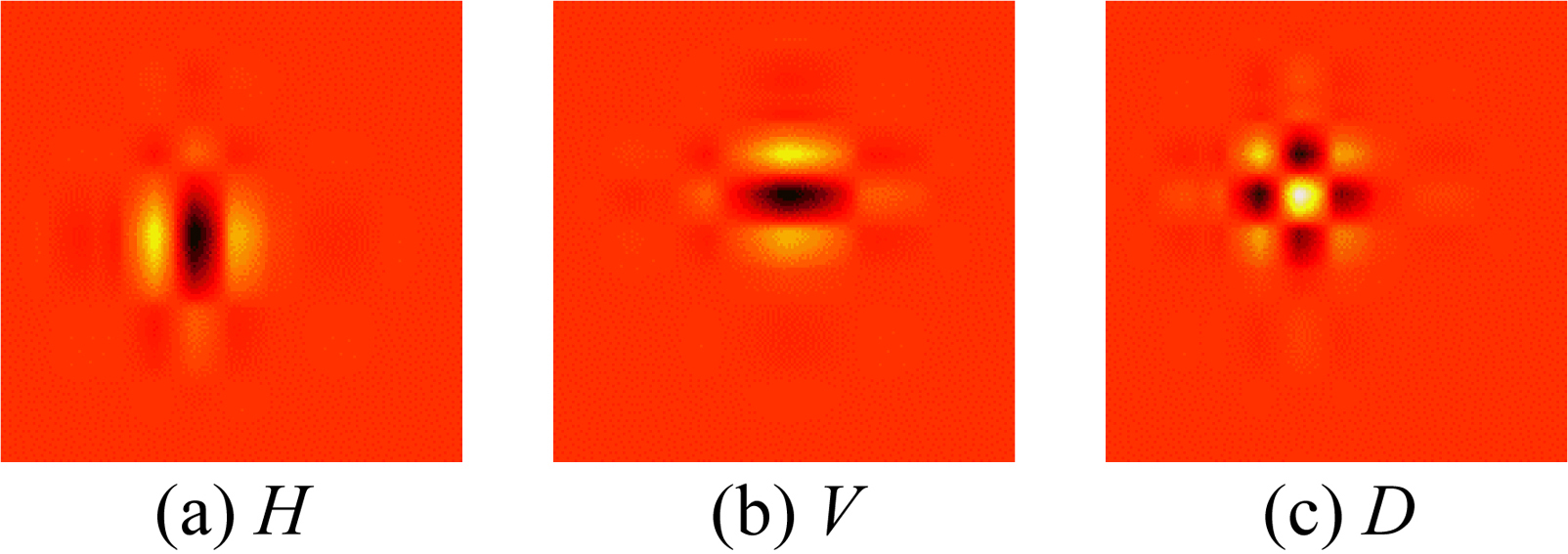 $H$ , $V$ , and $D$ represent horizontal, vertical, and diagonal, respectively).

Figure 8.

Directional selectivity of DTCWT.

Figure 9.

Directional selectivity of DDDTCWT.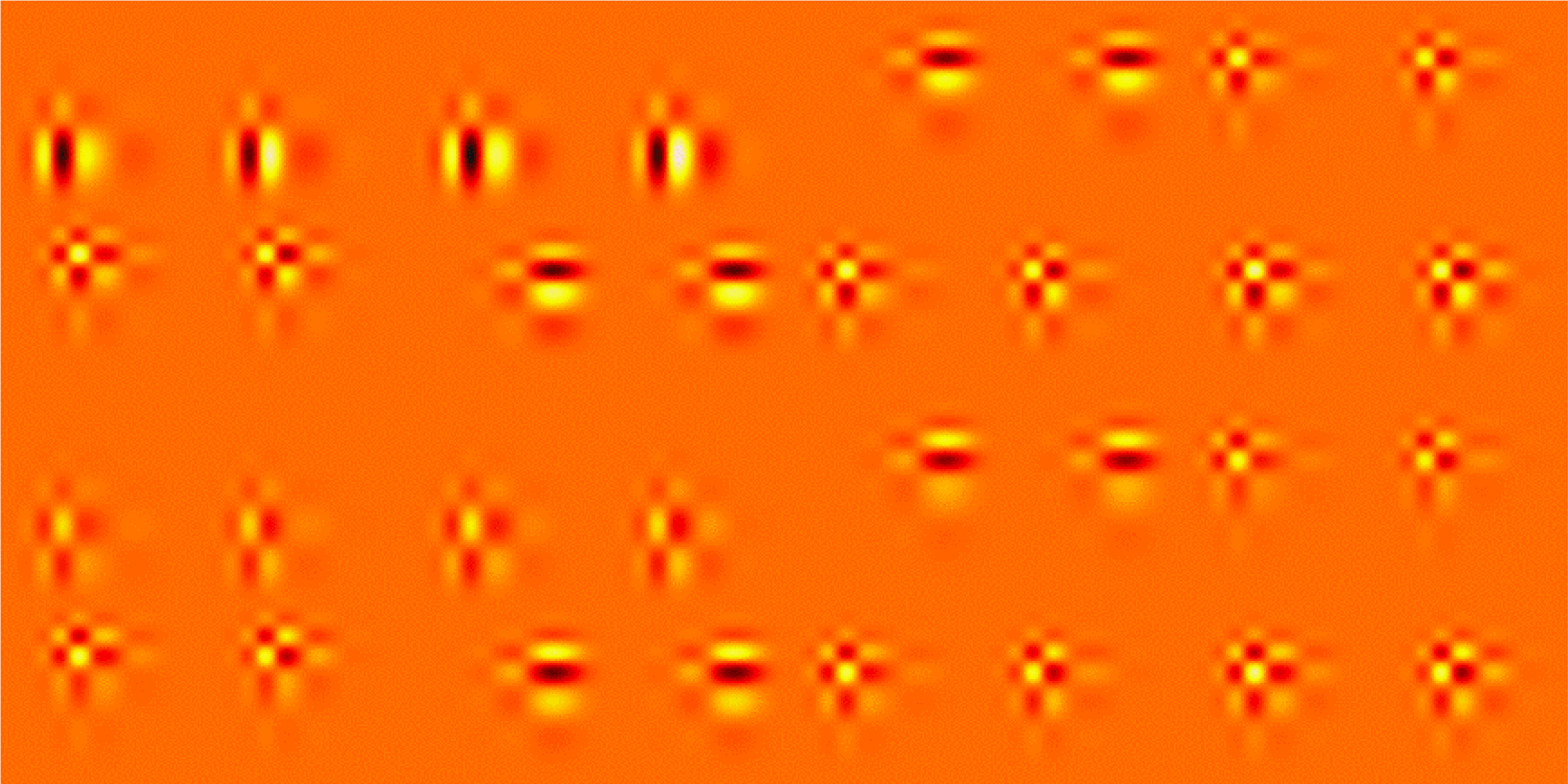

7.2 Reconstruction comparison

We performed a comparison between standard DWT, DTCWT, and DDDTCWT over a decagon simulation image shown in Fig. 10a. Next, the decagon image was decomposed at a 4-level decomposition. Their reconstruction was performed based on the 4-th level detail subband. Figure 10b–d gives the DWT reconstruction, DTCWT reconstruction, and DDDTCWT reconstruction, respectively.

We can observe easily from Fig. 10 that the DTCWT yields better edge reconstruction than DWT. The DWT reconstruction has a discontinued edge, and yet the DTCWT reconstruction has a clear and solid contour line. In addition, the DTCWT has some aliases along the borders and suffers from slight checkerboard effect. While DDDTCWT solved above problems well. This result suggests us the superiority of DDDTCWT.

Figure 10.

The reconstruction comparison between DWT and DTCWT.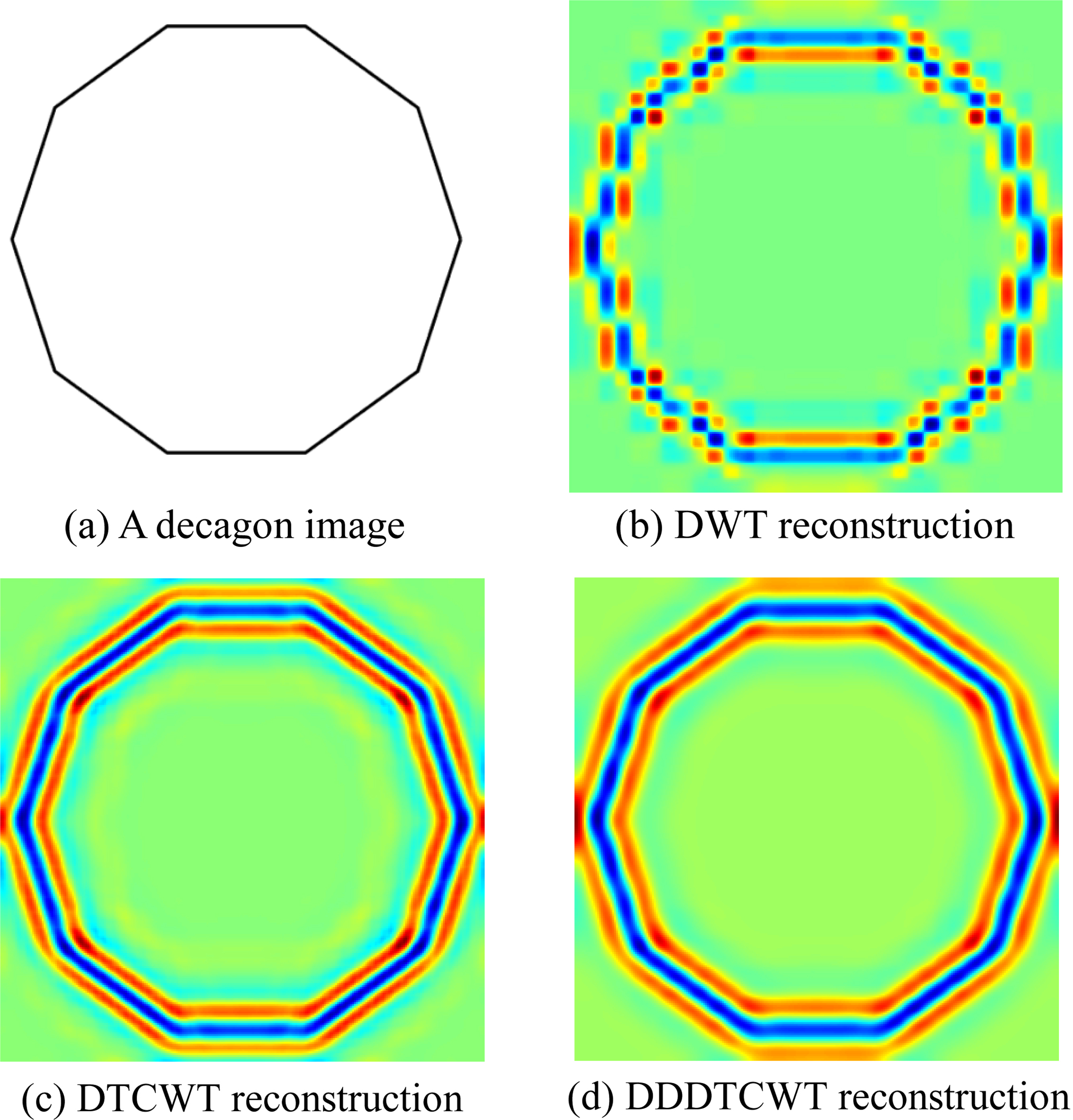

7.3 PCA versus KPCA

In the second experiment, we carried out a comparison among PCA, PKPCA, and RKPCA. Figure 11a shows the simulation data. Suppose we have three categories, and the number of each category is 361. The points in Class 1 lie in a sphere with radius of 1. The points in Class 2 lie in a sphere with radius of 2. The points of Class 3 lie in a sphere with a radius of 3.5. The original matrix size is 3249.

Figure 11b shows the PCA result, and Fig. 11c shows the PKPCA results. The results suggest 2PCs selected by either PCA or PKPCA cannot segment different classes. Figure 11d and e shows the RKPCA result, which indicates that even 1 PC selected by RKPCA can segment the three classes. Table 3 shows whether it is separable via difference PCA.

Figure 11.

KPCA versus PCA (here C1, C2, C3 represents the first class, second class, and third class, respectively).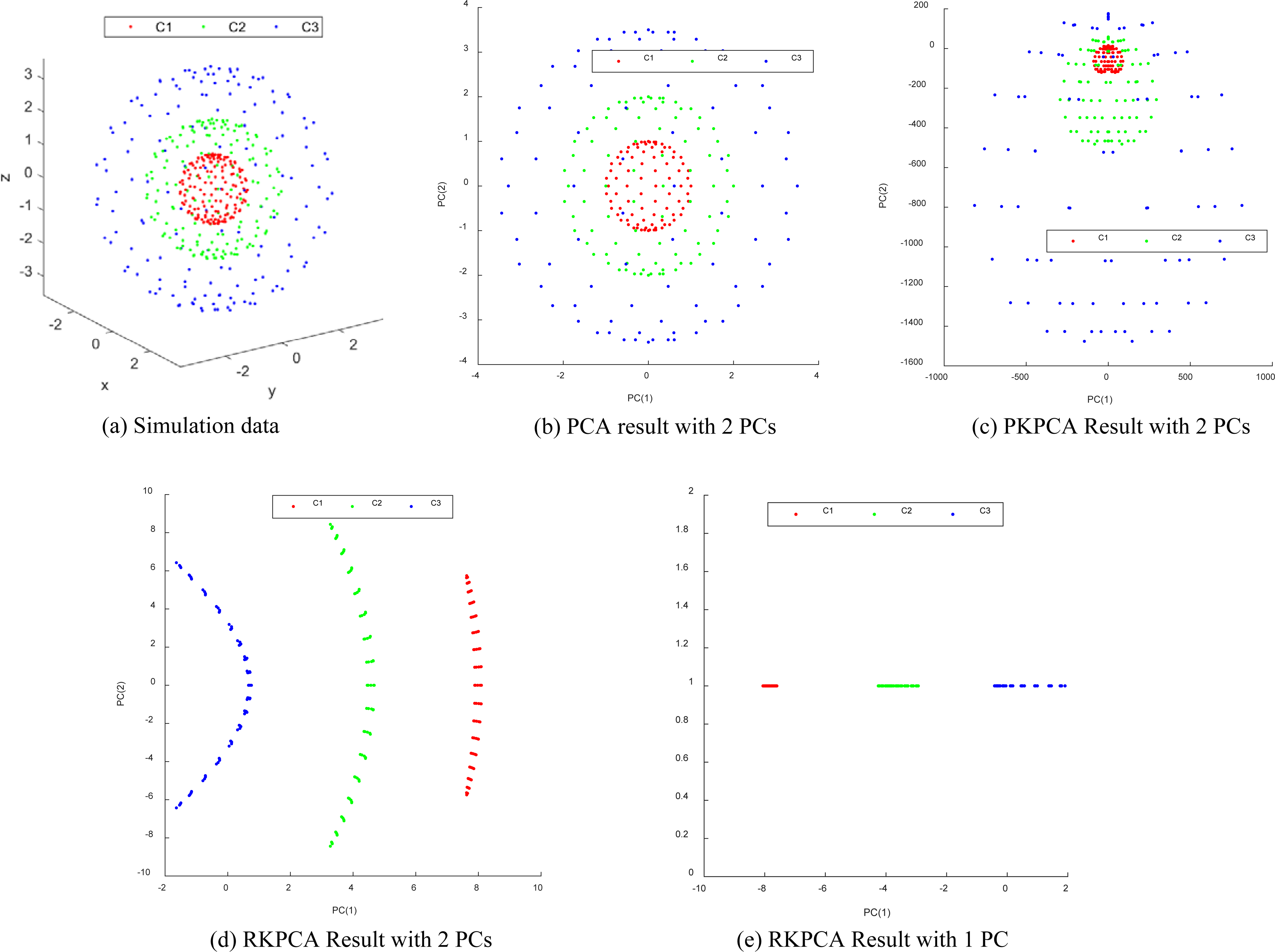

Table 2

The matrix size of the application of PCA

Methods	Matrix size
Simulation data	1083*3
PCA result with 2 PCs	1083*2
PKPCA result with 2 PCs	1083*2
RKPCA result with 2 PCs	1083*2
RKPCA result with 1 PC	1083*1

Table 2 shows the original size of the simulation data as 1083*3, after different types of PCA, the data can be reduced to either 1083*2 and 1083*1.

Table 3

Linear separability (X means inseparable, $\surd$ means separable)

	2 PCs	1 PC
PCA	X	X
PKPCA	X	X
RKPCA (ours)	$\surd$	$\surd$

8. Experiments on realistic data

In the experiment, our method used the following setting by the grid searching method. We used three-level DDDTCWT and used RKPCA with threshold of 99% of total variance. Our results were compared to eight state-of-the-art approaches. The 10 repetitions of 10-fold cross validation were used. The overall accuracy was used as the measure.

8.1 Decomposition of DDDTCWT

Take the photo in Fig. 3c as an example, we show its 1-level and 2-level DDDTCWT results in Figs 12 and 13, respectively. In each figure, the first column shows the real part of tree 1, the second column shows the imaginary part of tree 2, the third and last column shows the real and imaginary part of tree 2, respectively. Obviously, each level decomposition will generate 32 sub-bands (eight orientations multiplied by two trees multiplied by two parts).

Figure 12.

One-level DDDTCWT decomposition.

Figure 13.

Two-level DDDTCWT decomposition.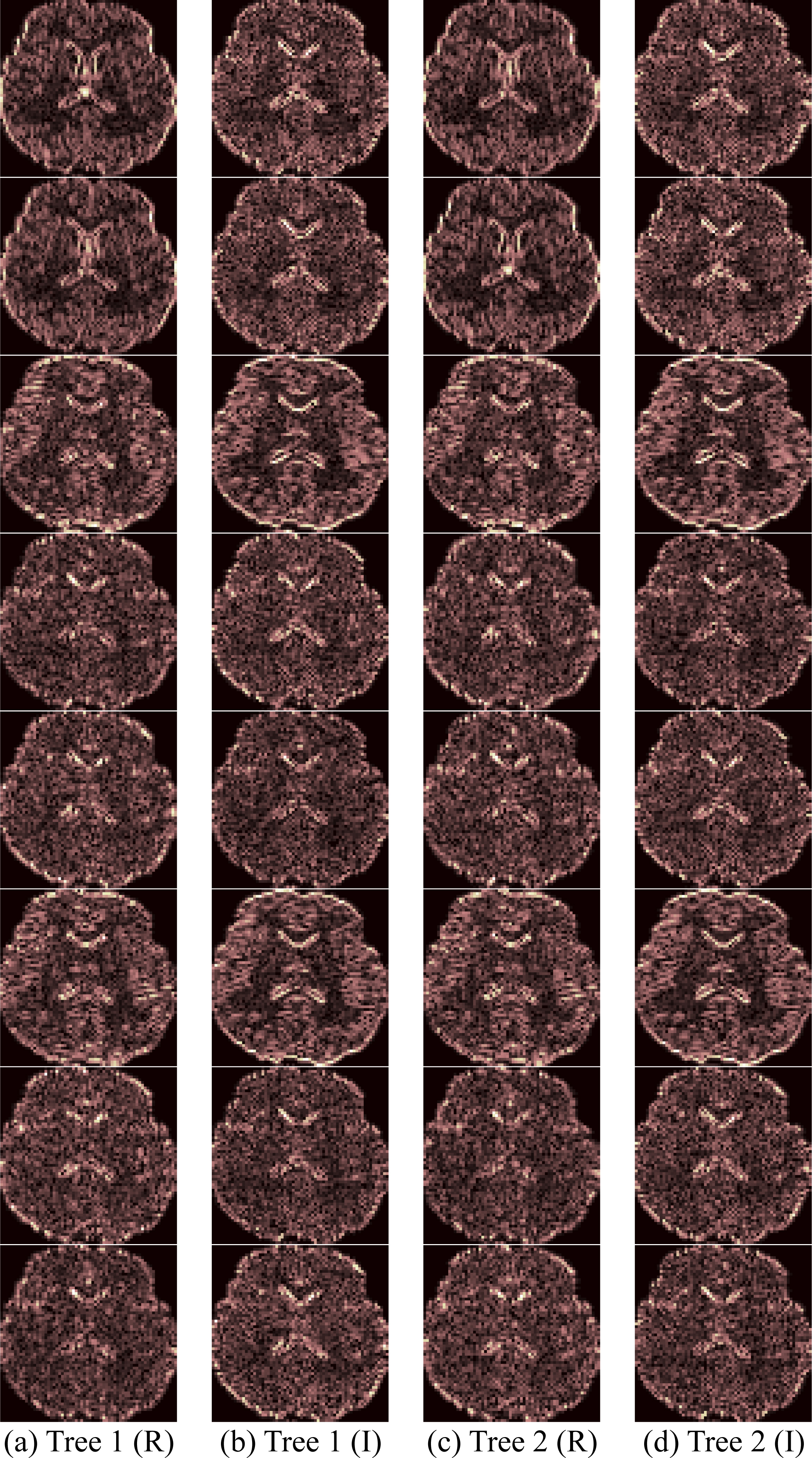

8.2 10 runs of 10-fold cross validation

Considering the dataset sample is small, the cross validation was employed to validate the proposed method. The 10 $\times$ 10-fold stratified cross validation results of our proposed method are listed below in Table 4. In this study, we set the C1, C2, and C3 as LSHL, RSHL, and HC, respectively.

Table 4
10 runs of 10-fold stratified cross validation

	F1	F2	F3	F4	F5	F6	F7	F8	F9	F10	Total
R1	3 $+$ 3 $+$ 3 $=$ 9	2 $+$ 3 $+$ 3 $=$ 8	3 $+$ 3 $+$ 3 $=$ 9	3 $+$ 3 $+$ 2 $=$ 8	3 $+$ 2 $+$ 3 $=$ 8	3 $+$ 3 $+$ 3 $=$ 9	3 $+$ 3 $+$ 2 $=$ 8	3 $+$ 3 $+$ 3 $=$ 9	3 $+$ 3 $+$ 3 $=$ 9	3 $+$ 3 $+$ 3 $=$ 9	29 $+$ 29 $+$ 28 $=$ 86
R2	3 $+$ 3 $+$ 2 $=$ 8	3 $+$ 3 $+$ 3 $=$ 9	3 $+$ 3 $+$ 3 $=$ 9	3 $+$ 3 $+$ 3 $=$ 9	3 $+$ 3 $+$ 3 $=$ 9	3 $+$ 3 $+$ 3 $=$ 9	3 $+$ 3 $+$ 3 $=$ 9	3 $+$ 3 $+$ 3 $=$ 9	3 $+$ 3 $+$ 3 $=$ 9	2 $+$ 3 $+$ 3 $=$ 8	29 $+$ 30 $+$ 29 $=$ 88
R3	2 $+$ 3 $+$ 3 $=$ 8	3 $+$ 3 $+$ 3 $=$ 9	3 $+$ 3 $+$ 3 $=$ 9	3 $+$ 3 $+$ 3 $=$ 9	3 $+$ 3 $+$ 3 $=$ 9	3 $+$ 3 $+$ 3 $=$ 9	3 $+$ 3 $+$ 3 $=$ 9	3 $+$ 3 $+$ 3 $=$ 9	2 $+$ 3 $+$ 2 $=$ 7	3 $+$ 3 $+$ 3 $=$ 9	28 $+$ 30 $+$ 29 $=$ 87
R4	3 $+$ 3 $+$ 3 $=$ 9	3 $+$ 3 $+$ 3 $=$ 9	3 $+$ 3 $+$ 3 $=$ 9	3 $+$ 3 $+$ 3 $=$ 9	3 $+$ 2 $+$ 3 $=$ 8	3 $+$ 3 $+$ 3 $=$ 9	3 $+$ 3 $+$ 3 $=$ 9	3 $+$ 2 $+$ 2 $=$ 7	3 $+$ 3 $+$ 3 $=$ 9	3 $+$ 3 $+$ 3 $=$ 9	30 $+$ 28 $+$ 29 $=$ 87
R5	3 $+$ 3 $+$ 3 $=$ 9	3 $+$ 3 $+$ 3 $=$ 9	3 $+$ 3 $+$ 3 $=$ 9	3 $+$ 3 $+$ 2 $=$ 8	3 $+$ 3 $+$ 3 $=$ 9	3 $+$ 3 $+$ 2 $=$ 8	3 $+$ 3 $+$ 3 $=$ 9	3 $+$ 3 $+$ 3 $=$ 9	3 $+$ 3 $+$ 3 $=$ 9	3 $+$ 3 $+$ 3 $=$ 9	30 $+$ 30 $+$ 28 $=$ 88
R6	2 $+$ 2 $+$ 3 $=$ 7	3 $+$ 3 $+$ 3 $=$ 9	3 $+$ 3 $+$ 3 $=$ 9	3 $+$ 3 $+$ 3 $=$ 9	3 $+$ 3 $+$ 3 $=$ 9	3 $+$ 2 $+$ 3 $=$ 8	3 $+$ 3 $+$ 3 $=$ 9	3 $+$ 3 $+$ 3 $=$ 9	3 $+$ 3 $+$ 3 $=$ 9	3 $+$ 2 $+$ 3 $=$ 8	29 $+$ 27 $+$ 30 $=$ 86
R7	3 $+$ 3 $+$ 2 $=$ 8	3 $+$ 3 $+$ 3 $=$ 9	3 $+$ 3 $+$ 3 $=$ 9	3 $+$ 3 $+$ 3 $=$ 9	3 $+$ 3 $+$ 2 $=$ 8	3 $+$ 3 $+$ 2 $=$ 8	3 $+$ 3 $+$ 2 $=$ 8	3 $+$ 3 $+$ 3 $=$ 9	3 $+$ 3 $+$ 3 $=$ 9	3 $+$ 3 $+$ 3 $=$ 9	30 $+$ 30 $+$ 26 $=$ 86
R8	3 $+$ 2 $+$ 3 $=$ 8	3 $+$ 3 $+$ 3 $=$ 9	1 $+$ 3 $+$ 3 $=$ 7	3 $+$ 3 $+$ 3 $=$ 9	3 $+$ 3 $+$ 3 $=$ 9	3 $+$ 3 $+$ 3 $=$ 9	3 $+$ 3 $+$ 3 $=$ 9	3 $+$ 3 $+$ 3 $=$ 9	3 $+$ 3 $+$ 3 $=$ 9	3 $+$ 3 $+$ 3 $=$ 9	28 $+$ 29 $+$ 30 $=$ 87
R9	2 $+$ 3 $+$ 3 $=$ 8	3 $+$ 3 $+$ 3 $=$ 9	3 $+$ 3 $+$ 3 $=$ 9	3 $+$ 3 $+$ 3 $=$ 9	2 $+$ 3 $+$ 3 $=$ 8	3 $+$ 3 $+$ 3 $=$ 9	3 $+$ 3 $+$ 3 $=$ 9	3 $+$ 3 $+$ 3 $=$ 9	3 $+$ 3 $+$ 2 $=$ 8	3 $+$ 2 $+$ 3 $=$ 8	28 $+$ 29 $+$ 29 $=$ 86
R10	2 $+$ 2 $+$ 3 $=$ 7	3 $+$ 3 $+$ 3 $=$ 9	3 $+$ 3 $+$ 3 $=$ 9	3 $+$ 3 $+$ 3 $=$ 9	3 $+$ 3 $+$ 3 $=$ 9	3 $+$ 3 $+$ 3 $=$ 9	3 $+$ 3 $+$ 3 $=$ 9	3 $+$ 3 $+$ 3 $=$ 9	3 $+$ 2 $+$ 3 $=$ 8	3 $+$ 3 $+$ 3 $=$ 9	29 $+$ 28 $+$ 30 $=$ 87
Total											290 $+$ 290 $+$ 288 $=$ 868

$a+b+c=d$ represents $a$ , $b$ , and $c$ samples are correctly identified as C1, C2, and C3, respectively. $d$ is the number of total corrected samples.

The sensitivities of each class based on 10 runs are offered in Table 5. Here we see the LSHL has a sensitivity of 96.67 $\pm$ 2.72%, the RSHL has a sensitivity of 96.67 $\pm$ 3.51%, and the healthy control has a sensitivity of 96.00 $\pm$ 4.10%.

Table 6 gives the overall accuracy based on 10 runs. It shows that our method achieves an average accuracy with value of 96.44 $\pm$ 0.88%.

Table 5

Sensitivities of each class (unit: %)

	C1	C2	C3
R1	96.67	96.67	93.33
R2	96.67	100.00	96.67
R3	93.33	100.00	96.67
R4	100.00	93.33	96.67
R5	100.00	100.00	93.33
R6	96.67	90.00	100.00
R7	100.00	100.00	86.67
R8	93.33	96.67	100.00
R9	93.33	96.67	96.67
R10	96.67	93.33	100.00
Average	96.67 $\pm$ 2.72	96.67 $\pm$ 3.51	96.00 $\pm$ 4.10

Table 6

The overall accuracy (unit: %)

	Accuracy
R1	95.56
R2	97.78
R3	96.67
R4	96.67
R5	97.78
R6	95.56
R7	95.56
R8	96.67
R9	95.56
R10	96.67
Average	96.44 $\pm$ 0.88

8.3 Comparison of decomposition level and feature extraction methods

We tested the performance of DWT, DTCWT, and DDDTCWT, and let their corresponding decomposition level ( $L$ ) vary from 1 to 5 with increment of 1. The results are presented in Table 7, and a graphical chart is shown in Fig. 14.

Table 7
Overall accuracy of different decomposition levels and different feature extraction methods (Unit: %)

Feature extraction	$L=$ 1	$L=$ 2	$L=$ 3	$L=$ 4	$L=$ 5
DWT	90.44	92.44	93.22	93.56	92.56
DTCWT	93.33	94.56	96.11	95.11	94.89
DDDTCWT	92.44	95.78	96.44	95.33	95.44
(proposed)

Figure 14.

Select the best feature extraction method and the optimal decomposition level.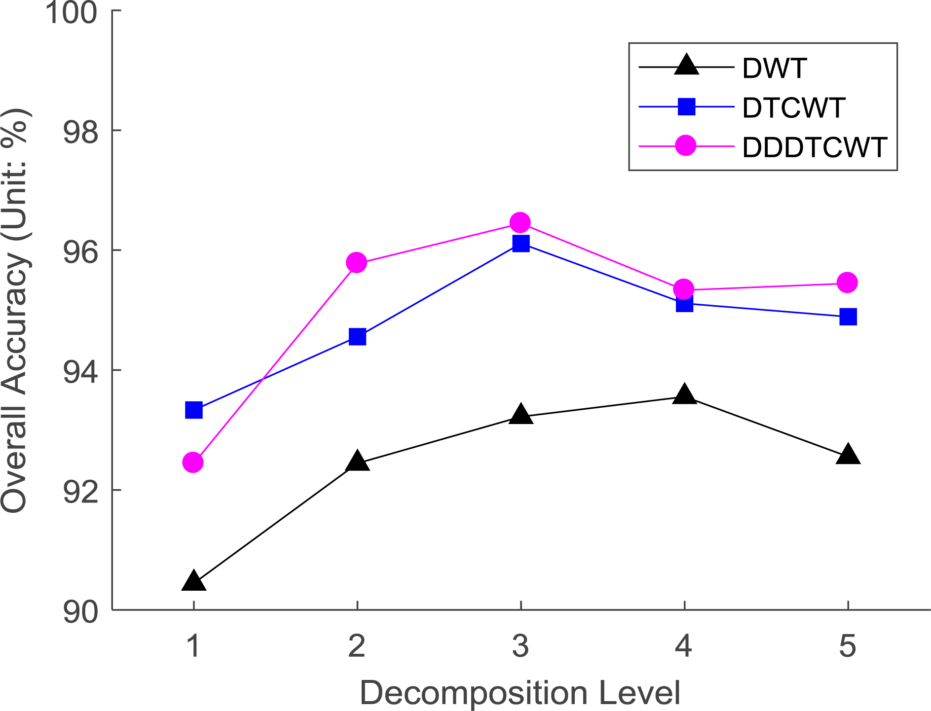

Figure 14 shows the overall accuracy under different decomposition levels and different feature extraction methods. As is seen, the best decomposition level for DWT is 4, and the best decomposition level for DTCWT and DDDTCWT are three. The reason may be two folds: On one hand, more decomposition level will give better analysis of the brain image. On the other hand, too large decomposition level will introduce calculation error, thus decreasing the performance. In all, we found from Fig. 14 that 3-level DDDTCWT achieves the highest overall accuracy than other settings.

8.4 Optimal setting of feature reduction

In this experiment, we compared PCA, PKPCA and RKPCA at different thresholds ( $T$ ): 90%, 95%, 99% and 99.9% respectively. Other parameters kept same during this experiment, i.e., we still use 3-level DDDTCWT as the feature extraction method. The results are listed in Table 8 and the picture is presented in Fig. 15.

Table 8
Overall accuracy of different feature reduction methods with different threshold setting

Feature	$T=$ 90%	$T=$ 95%	$T=$ 99%	$T=$ 99.9%
reduction
PCA	94.33	94.78	95.00	95.11
PKPCA	94.56	96.00	96.22	95.89
RKPCA	95.00	96.11	96.44	95.78

Figure 15 shows that the optimal feature reduction method is to use RKPCA with threshold as 0.99. The superiority of RKPCA to PCA and PKPCA is in line with the simulation result in Section 7.3. The RKPCA has a better capability of mapping data from linear space to nonlinear space, so as to unwrap the interwoven data.

8.5 Classifier comparison

In this experiment, we compared the MLR with other commonly used classifiers, including C5.0 decision tree (DT), support vector machine (SVM) [53], and back propagation neural network (BPNN) [54]. The features were obtained by (i) three-level DDDT CWT, and (ii) RKPCA with threshold of 99% of total variance. The overall accuracy of 10 $\times$ 10-fold cross validation of all methods were listed in Table 9.

Table 9
Classifier comparison

Classifier	Overall accuracy
DT	86.67 $\pm$ 1.74%
SVM	94.11 $\pm$ 1.05%
BPNN	92.56 $\pm$ 1.39%
MLR (proposed)	96.44 $\pm$ 0.88%

Figure 15.

Select the best feature reduction method with optimal threshold.

The overall accuracy results of different classifiers in Table 9 show that our MRL method got the best overall accuracy, and the least standard deviation (only 0.88), although it is a rather old technique. In addition, the SVM obtained an overall accuracy of 94.11 $\pm$ 1.05%, the BPNN obtained an overall accuracy of 92.56 $\pm$ 1.39%, and the DT performed worst with the lowest overall accuracy and largest standard deviation of 86.67 $\pm$ 1.74%. Nevertheless, Du et al. [55], Bui et al. [56], and Khoja et al. [57] all reported situations where (multinomial) logistic regression gives better performances than latest classifiers. Hence, this result gives us an indication that even old method (like MLR) can give a better result.

Currently, MLR is also widely applied in the last layer of the convolutional neural network, which is the most successful tool in the field of deep learning. Therefore, we cannot refer SVM is better or MLR is better without considering the exact problems. In this paper, we applied the algorithm to a multi classification problem. According to the test based on our dataset, the MLR outperforms the SVM.

8.6 Comparison with AlexNet

Table 10
Statistical analysis (Unit: %)

	AlexNet	AlexNet	Ours
	(raw) [58]	(improved) [59]
R1	92.22	94.44	95.56
R2	92.22	96.67	97.78
R3	94.44	95.56	96.67
R4	92.22	95.56	96.67
R5	91.11	93.33	97.78
R6	95.56	96.67	95.56
R7	92.22	94.44	95.56
R8	95.56	95.56	96.67
R9	93.33	95.56	95.56
R10	92.22	94.44	96.67
$P$ value	0.0039 $<$ 0.05	0.0234 $<$ 0.05

Table 10 shows the accuracy performed by AlexNet (raw), AlexNet (improved) and our proposed method. In order to validate our proposed method, we test the statistical significance for our method. The $p$ value in the 2-group as 0.0039 for AlexNet (raw) and Our method, 0.0234 for AlexNet (improved) and our proposed method. As both $p$ values are less than 0.05, which indicates the statistical significance of the performance of our proposed method.

In this experiment, we compared our method with AlexNet [58], which is a well-pretrained 25-layer neural network in the field of deep learning. The AlexNet model in Matlab is trained on a subset of ImageNet database, and it can classify 1000 object categories (for instance, pencil, mouse, keyboard, etc.). We invoked the model by Matlab command of “alexnet” and compared with our method. The parameter settings were the same as previous sections. The raw AlexNet [58] and improved AlexNet [59] are both tested in this experiment. The improved AlexNet retrains the last three layers.

Table 11

Comparison to AlexNet

Method	Overall accuracy
AlexNet (raw) [58]	93.11 $\pm$ 1.55%
AlexNet (improved) [59]	95.22 $\pm$ 1.05%
DDDTCWT $+$ RKPCA $+$ MLR (our)	96.44 $\pm$ 0.88%

Table 12

Algorithm comparison based on 10-fold cross validation over our 90-image dataset

Method	Overall accuracy	Rank
FRFT $+$ PCA $+$ SFN [10]	95.11%	4
WPD $+$ LS-SVM [11]	95.44%	3
WE $+$ DAG-SVM [12]	95.11%	4
DWT $+$ PCA $+$ SVM [13]	94.11%	6
DWT $+$ PCA $+$ GEPSVM [13]	92.22%	7
WPE $+$ BP [18]	87.11%	8
HMI [19]	77.44%	9
DTCWT $+$ KPCA $+$ MLR [21]	96.11%	2
DDDTCWT $+$ RKPCA $+$ MLR	96.44 $\pm$ 0.88%	1
(proposed)

Here we see that raw AlexNet [58] gives an overall accuracy of only 93.11%, and the improved Alex-Net [59] yields an overall accuracy of 95.22%. Both methods perform less than our MLR method of 96.44%. The reason is three folds. First, the raw AlexNet [58] is pretrained to identify natural images, and our MLR method is trained particularly to accomplish the hearing loss identification task. Second, raw AlexNet [58] can identify 1000 types of objects, but none of them are brain magnetic resonance images. Third, retraining AlexNet [59] usually needs a median-size dataset, but our 90-image dataset is too small in terms of size, due to the difficulty of collecting more medical data. Therefore, our method can give better performance than both raw and fine-trained pretrained CNN. This suggests that hand engineering is still quite important in classification on small-size dataset.

8.7 Comparison to state-of-the-art approaches

Table 12 offers our proposed method with eight methods: FRFT $+$ PCA $+$ SFN [10], WPD $+$ LS-SVM [11], WE $+$ DAG-SVM [12], DWT $+$ PCA $+$ SVM [13], DWT $+$ PCA $+$ GEPSVM [13], WPE $+$ BP [18], HMI [19], and DTCWT $+$ KPCA $+$ MLR [21]. All the results were obtained by our in-house programming over the same dataset with the same cross validation settings.

The comparison results in Table 12 show that our proposed DDDTCWT $+$ RKPCA $+$ MLR method yielded the largest accuracy of 96.44%. Next is DTC WT $+$ KPCA $+$ MLR [21] with an overall accuracy of 96.11%. The third is WPD $+$ LS-SVM [11] algorithm that yielded an accuracy of 95.44%. Both FRFT $+$ PCA $+$ SFN [10] and WE $+$ DAG-SVM [12] ranked fourth with an accuracy of 95.11%. The DWT $+$ PCA $+$ SVM [13] ranked the sixth with an accuracy of 94.11%. DWT $+$ PCA $+$ GEPSVM [13] performed the seventh, and WPE $+$ BP [18] performed the eighth. Finally, HMI [19] yielded the worst result.

As three main advantages of DDDTCWT are summarized in Patil et al. [37]: (i) double-density wavelets; (ii) directional-selectivity; (iii) shift-invariance. Those advantages guarantee that DDDTCWT will provide better performances than either DWT or DTCWT.

8.8 Time analysis

We used our trained classifier on 1000 new brain images and calculated the average time. The computation time on CPU and GPU at each stage is listed in Table 13.

Table 13
Time analysis for predicting a new brain image

Stage	CPU time	GPU time	Acceleration
	(unit: millisecond)	(unit: millisecond)
DDDTCWT	24.98	0.83	30x
PC coefficient extraction	5.71	0.16	36x
MLR prediction	2.96	0.07	42x
Total	33.65	1.06	32x

8.9 Validation of optimal slice

This experiment aimed to seek the optimal slice from $Z=$ 30 to $Z=$ 150. The settings are the same as previous Sections: We used three-level DDDTCWT and used RKPCA with threshold of 99% of total variance. We used 10 repetition of 10-fold cross validation was used. The overall accuracy was pictured in Fig. 16.

Figure 16.

Overall accuracy changes with selected slice.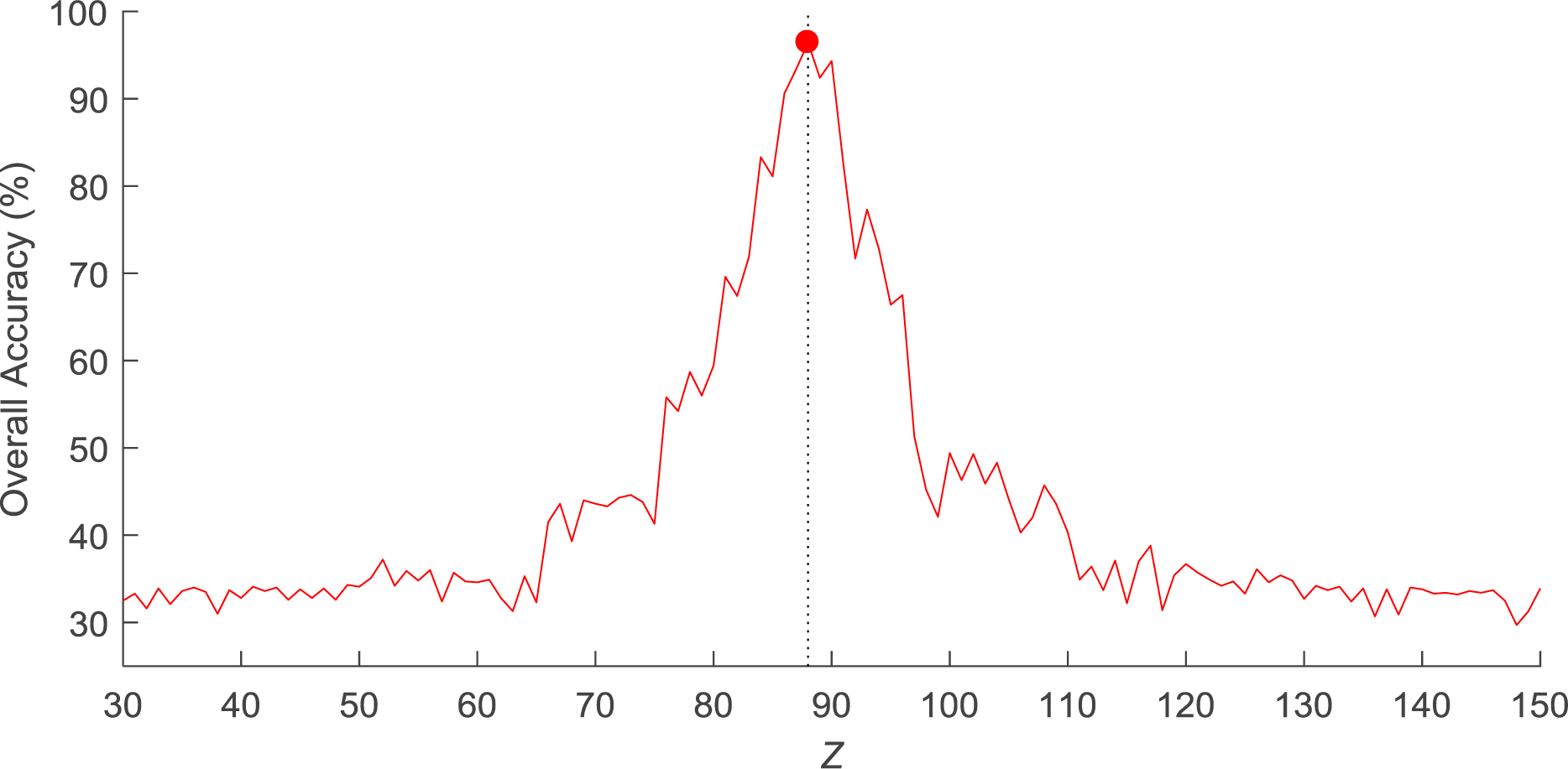

Here we can see from Fig. 16 that, 88-th slice achieves the highest overall accuracy. This is in line with the result suggested by experienced radiologists. It indicates that 88-th slice contains the most distinguishing brain tissues between left hearing loss, right hearing loss, and healthy control. The lobe containing 88-th slice shows that the neighboring slices of 88-th slice also contribute to the identification but are not as efficient as 88-th slice. For those slices far away from 88-th slice, the overall accuracy decreased to 33.3%, which is the overall accuracy for a random-guess classifier for a three-class task.

Nevertheless, the optimal slice may be chosen vertical to $X$ or $Y$ axes, or it can be even an oblique plane to all three axes. Here we choose a slice vertical to $Z$ axis, is for the ease of radiologists since they usually read the axial slices. In the future, we shall develop techniques to handle with multi-slices, and we may develop surface analysis techniques.

9. Conclusion

In this study, we proposed a novel unilateral sensorineural hearing-loss detection method, which can identify left-sided hearing loss and right-sided hearing loss from healthy controls. Our method is based on three successful techniques: double-density dual-tree complex wavelet transform, kernel principal component analysis, and multinomial logistic regression. The results showed our method is superior to both raw and improved AlexNet, and eight state-of-the-art approaches.

In the future, we may apply our method to other brain disease detection, such as Alzheimer’s disease and Parkinson’s disease, etc. Other research directions contain multi-slice processing and surface analysis.

Footnotes

Acknowledgments

This paper was supported by Natural Science Foundation of China (61602250), Natural Science Foundation of Jiangsu Province (BK20150983, BK20150982), Program of Natural Science Research of Jiangsu Higher Education Institutions (16KJB520025), and the MIN ECO under the TEC2015-64718-R project, the Salvador de Madariaga Mobility Grants 2017 and the Consejería de Economía, Innovación, Ciencia y Empleo (Junta de Andalucía, Spain) under the Excellence Project P11-TIC-7103.

References

Fakhim

Naderpoor

Shahidi

Basharhashemi

Nejati

Sakha

, et al. Study of prevalence and causes of hearing loss in high risk neonates admitted to neonatal ward and neonatal intensive care unit. Journal of International Advanced Otology. 2010; 6(3): 365-70.

Pinninti

Rodgers

Novak

Britt

Fowler

Boppana

, et al. Clinical predictors of sensorineural hearing loss and cognitive outcome in infants with symptomatic congenital cytomegalovirus infection. Pediatric Infectious Disease Journal. 2016; 35(8): 924-6.

Killeen

Hefferly

Hodge

Balk

. Assessment of hearing loss and balance among adult cf patients exposed to potential ototoxic medications. Pediatric Pulmonology. 2015; 50: 340-1.

Paraouty

Ewert

Wallaert

Lorenzi

. Interactions between amplitude modulation and frequency modulation processing: Effects of age and hearing loss. Journal of the Acoustical Society of America. 2016; 140(1): 121-31.

Masterson

Howard

Liu

Phillips

. Asymmetrical hearing loss in cases of industrial noise exposure: A systematic review of the literature. Otology & Neurotology. 2016; 37(8): 998-1005.

Bas

Bohorquez

Goncalves

Perez

Dinh

Garnham

, et al. Electrode array-eluted dexamethasone protects against electrode insertion trauma induced hearing and hair cell losses, damage to neural elements, increases in impedance and fibrosis: A dose response study. Hearing Research. 2016; 337: 12-24.

Lidian

Linder

Anniko

Nordang

. BDNF as otoprotectant in toxin-induced hearing loss. Acta Oto-Laryngologica. 2013; 133(1): 4-11.

Parker

. Biotechnology in the treatment of sensorineural hearing loss: Foundations and future of hair cell regeneration. Journal of Speech Language and Hearing Research. 2011; 54(6): 1709-31.

Mirzaei

Adeli

. Segmentation and clustering in brain MRI imaging. Reviews in the Neurosciences. 2018; 30(1): 31-44.

10.

. Detection of left-sided and right-sided hearing loss via fractional fourier transform. Entropy. 2016; 18(5): 194.

11.

Chen

. Computer-aided detection of left and right sensorineural hearing loss by wavelet packet decomposition and least-square support vector machine. Journal of the American Geriatrics Society. 2016; 64(S2): S350.

12.

Gorriz

Ramírez

. Wavelet entropy and directed acyclic graph support vector machine for detection of patients with unilateral hearing loss in MRI scanning. Front Comput Neurosci. 2016; 10: 160.

13.

Chen

X-Q

. Sensorineural hearing loss detection via discrete wavelet transform and principal component analysis combined with generalized eigenvalue proximal support vector machine and tikhonov regularization. Multimedia Tools and Applications. 2016; 77(3): 3775-93.

14.

Sun

. Preliminary research on abnormal brain detection by wavelet-energy and quantum-behaved PSO. Technology and Health Care. 2016; 24(s2): S641-S9.

15.

. Smart detection on abnormal breasts in digital mammography based on contrast-limited adaptive histogram equalization and chaotic adaptive real-coded biogeography-based optimization. Simulation. 2016; 92(9): 873-85.

16.

. A pathological brain detection system based on radial basis function neural network. Journal of Medical Imaging and Health Informatics. 2016; 6(5): 1218-22.

17.

Chen

X-Q.

,Fractal dimension estimation for developing pathological brain detection system based on Minkowski-Bouligand method, IEEE Access. 2016; 4: 5937-47.

18.

, editor. Hearing loss detection in medical multimedia data by discrete wavelet packet entropy and single-hidden layer neural network trained by adaptive learning-rate back propagation. 14th International Symposium on Neural Networks (ISNN); Sapporo, Japan: Springer. 2017; 541-9.

19.

Pereira

. Hu moment invariant: A new method for hearing loss detection. Advances in Engineering Research. 2017; 153: 412-6.

20.

Jia

. Three-category classification of magnetic resonance hearing loss images based on deep autoencoder. Journal of Medical Systems. 2017; 41: 165.

21.

Wang

Zhang

Yang

Liu

Ramirez

Gorriz

. Preliminary study on unilateral sensorineural hearing loss identification via dual-tree complex wavelet transform and multinomial logistic regression. in: Natural and Artificial Computation for Biomedicine and Neuroscience: International Work-Conference on the Interplay Between Natural and Artificial Computation, IWINAC 2017, Corunna, Spain, June 19-23, 2017, Proceedings, Part I. Ferrández Vicente

Álvarez-Sánchez

de la Paz López

Toledo More

Adeli

, editors. Cham: Springer International Publishing. 2017; 289-97.

22.

Smith

. Fast robust automated brain extraction. Human Brain Mapping. 2002; 17(3): 143-55.

23.

Jenkinson

Smith

. A global optimisation method for robust affine registration of brain images. Medical Image Analysis. 2001; 5(2): 143-56.

24.

Jenkinson

Bannister

Brady

Smith

. Improved optimization for the robust and accurate linear registration and motion correction of brain images. Neuro Image. 2002; 17(2): 825-41.

25.

Woolrich

Jbabdi

Patenaude

Chappell

Makni

Behrens

, et al. Bayesian analysis of neuroimaging data in FSL. Neuro Image. 2009; 45(1, Supplement 1): S173-S86.

26.

Ahmadlou

Adeli

. Fuzzy synchronization likelihood-wavelet methodology for diagnosis of autism spectrum disorder. J Neurosci Methods. 2012; 211(2): 203-9.

27.

Sharma

Khan

Farooq

Tripathi

Adeli

. A wavelet-statistical features approach for nonconvulsive seizure detection. Clinical EEG and Neuroscience. 2014; 45(4): 274-84.

28.

Amezquita-Sanchez

Valtierra-Rodriguez

Adeli

Perez-Ramirez

. A novel wavelet transform-homogeneity model for sudden cardiac death prediction using ECG signals. J Med Syst. 2018; 42(10): 176.

29.

Ortiz-Rosario

Adeli

Buford

. Wavelet methodology to improve single unit isolation in primary motor cortex cells. J Neurosci Methods. 2015; 246: 106-18.

30.

Agustika

Triyana

, editors. Application of principal component analysis and discrete wavelet transform in electronic nose for herbal drinks classification. Advances of Science and Technology for Society; Melville: Amer Inst Physics. 2016; 198-203.

31.

Phillips

. Pathological brain detection in magnetic resonance imaging scanning by wavelet entropy and hybridization of biogeography-based optimization and particle swarm optimization. Progress in Electromagnetics Research. 2015; 152: 41-58.

32.

Abbasi

Bennet

Gunn

Unsworth

. Robust wavelet stabilized ‘footprints of uncertainty’ for fuzzy system classifiers to automatically detect sharp waves in the EEG after hypoxia ischemia. International Journal of Neural Systems. 2017; 27(3): 1650051.

33.

Yuan

Zhou

Leng

Wei

. Epileptic EEG identification via LBP operators on wavelet coefficients. Int J Neural Syst. 2018; 28(8): 1850010.

34.

Ahmadlou

Adeli

. Fractality and a wavelet-chaos-methodology for EEG-based diagnosis of alzheimer disease. Alzheimer Disease and Associated Disorders. 2011; 25(1): 85-92.

35.

Ravichandran

Selvakumar

. Multimodal medical image fusion using dual-tree complex wavelet transform (DTCWT) with modified lion optimization technique (mLOT) and intensity co-variance verification (ICV). Applied Computational Electromagnetics Society Journal. 2016; 31(6): 717-30.

36.

Yang

. Dual-tree complex wavelet transform and twin support vector machine for pathological brain detection. Applied Sciences. 2016; 6(6): 169.

37.

Patil

Kothari

Bhurchandi

. Expression invariant face recognition using local binary patterns and contourlet transform. Optik. 2016; 127(5): 2670-8.

38.

Ghosh-Dastidar

Adeli

Dadmehr

. Principal component analysis-enhanced cosine radial basis function neural network for robust epilepsy and seizure detection. IEEE Transactions on Bio-Medical Engineering. 2008; 55(2 Pt 1): 512-8.

39.

López

Ramírez

Górriz

Álvarez

Salas-Gonzalez

Segovia

, et al. Principal component analysis-based techniques and supervised classification schemes for the early detection of alzheimer’s disease. Neurocomputing. 2011; 74(8): 1260-71.

40.

. An MR brain images classifier via principal component analysis and kernel support vector machine. Progress in Electromagnetics Research. 2012; 130: 369-88.

41.

Mirea

Aivaz

, editors. Analyzing “the workforce cost” and “the net nominal earnings” in the main economic activities, by principal component analysis. Basiq International Conference – New Trends in Sustainable Business and Consumption; Konstanz, Germany: Editura ASE. 2016; 201-9.

42.

Adamiak

Duch

Zurek

Slot

, editors. Modifications of most expressive feature reordering criteria for supervised kernel principal component analysis. 2nd International Conference on Cybernetics (CYBCONF); Gdynia, POLAND: IEEE. 2015; 507-11.

43.

Rushin

Stancil

Sun

Adams

Beling

, editors. Horse race analysis in credit card fraud-deep learning, logistic regression, and gradient boosted tree. Systems and Information Engineering Design Symposium (SIEDS); Charlottesville, VA, USA: IEEE. 2017; 117-21.

44.

Franc

Zien

Schölkopf

, editors. Support vector machines as probabilistic models. International Conference on Machine Learning (ICML); Bellevue, United States. 2011; 665-72.

45.

Zhang

Y-D

Pan

Sun

Tang

. Multiple sclerosis identification by convolutional neural network with dropout and parametric reLU. Journal of Computational Science. 2018; 28: 1-10.

46.

Pan

. Abnormal breast identification by nine-layer convolutional neural network with parametric rectified linear unit and rank-based stochastic pooling. Journal of Computational Science. 2018; 27: 57-68.

47.

Y-D

. Alcoholism detection by data augmentation and convolutional neural network with stochastic pooling. Journal of Medical Systems. 2018; 42(1): 2.

48.

Pramesti

Damayanti

Asfani

, editors. Stator fault identification analysis in induction motor using multinomial logistic regression. International Seminar on Intelligent Technology and its Applications (ISITIA); Lombok, Indonesia: IEEE. 2016; 439-42.

49.

Lee

Piao

Shi

Choi

, editors. New approaches to identify cancer heterogeneity in DNA methylation studies using the lepage test and multinomial logistic regression. IEEE Conference on Computational Intelligence in Bioinformatics and Computational Biology (CIBCB); Honolulu, HI: IEEE. 2015; 73-9.

50.

Quan

Jeong

. A fast discrete wavelet transform using hybrid parallelism on GPUs. IEEE Trans Parallel Distrib Syst. 2016; 27(11): 3088-100.

51.

Luo

, editors. GPu-based parallel kernel PCA feature extraction for hyperspectral images. International Conference on Remote Sensing and Wireless Communications (RSWC); Shanghai, PEOPLES R CHINA: DESTech. 2014; 140-5.

52.

Wang

Plaza

Sun

Wei

. Real-time implementation of the sparse multinomial logistic regression for hyperspectral image classification on GPUs. IEEE Geosci Remote Sens Lett. 2015; 12(7): 1456-60.

53.

Ding

Shi

. Discrete space reinforcement learning algorithm based on support vector machine classification. Pattern Recognition Letters. 2018; 111: 30-5.

54.

Chen

Wang

Ming

. Effective tourist volume forecasting supported by PCA and improved BPNN using baidu index. Tourism Management. 2018; 68: 116-26.

55.

Zhang

Iqbal

Yang

Yao

. Landslide susceptibility mapping using an integrated model of information value method and logistic regression in the bailongjiang watershed, gansu province, china. J Mt Sci. 2017; 14(2): 249-68.

56.

Bui

KTT

Nguyen

Revhaug

. Tropical forest fire susceptibility mapping at the cat ba national park area, hai phong city, vietnam, using GIS-based kernel logistic regression. Remote Sens. 2016; 8(4): 15: 347.

57.

Khoja

Chipulu

Jayasekera

. Analysing corporate insolvency in the gulf cooperation council using logistic regression and multidimensional scaling. Rev Quant Financ Account. 2016; 46(3): 483-518.

58.

Yuan

Zhang

. Feature extraction and image retrieval based on alexNet. Proceedings of SPIE. 2016; 10033: 100330E.

59.

Xiao

Yan

Deng

, editors. Scene classification with improved alexNet model. 12th International Conference on Intelligent Systems and Knowledge Engineering (ISKE); NanJing, PEOPLES R CHINA: IEEE. 2017; 57-62.

Unilateral sensorineural hearing loss identification based on double-density dual-tree complex wavelet transform and multinomial logistic regression

Abstract

AIM:

METHOD:

RESULT:

CONCLUSION:

Keywords

1. Introduction

2. Subjects

Table 1 Demographics of the 90-subject dataset

4.1 Discrete wavelet transform

5.1 Principal component analysis

5.2 Kernel PCA

6.1 Logistic regression model

7.1 Directional selectivity comparison

8.1 Decomposition of DDDTCWT

Table 4 10 runs of 10-fold stratified cross validation

Table 7 Overall accuracy of different decomposition levels and different feature extraction methods (Unit: %)

Table 8 Overall accuracy of different feature reduction methods with different threshold setting

Table 9 Classifier comparison

Table 10 Statistical analysis (Unit: %)

8.8 Time analysis

Table 13 Time analysis for predicting a new brain image

Footnotes

Acknowledgments

References

Table 1
Demographics of the 90-subject dataset

Table 4
10 runs of 10-fold stratified cross validation

Table 7
Overall accuracy of different decomposition levels and different feature extraction methods (Unit: %)

Table 8
Overall accuracy of different feature reduction methods with different threshold setting

Table 9
Classifier comparison

Table 10
Statistical analysis (Unit: %)

Table 13
Time analysis for predicting a new brain image