Routing in congested baggage handling systems using deep reinforcement learning

Abstract

The increasing number of people choosing to travel by airplane puts pressure on the baggage handling systems in airports. As the load increases, the risk of deadlocks in the systems increase as well. Therefore, it is increasingly important to find routing solutions which can handle the high loads. Currently this is achieved by using shortest path algorithms and hand engineered site-specific routing rules, based on the experience of the employees and on trial and error processes using complex emulators. This is a time-consuming and costly approach, as every airport needs its own set of routing rules.

New development within machine learning, and especially reinforcement learning allows very complex control policies to be found in large environments. This could therefore potentially solve the need of manually creating site-specific routing rules.

This paper proposes to use a single global deep reinforcement learning agent to route a fleet of baggage-totes to continuously pick up and deliver baggage in simple yet functionally realistic simulations of baggage handling systems. This is achieved using a Dueling DQN architecture with prioritized experience reply and a multi action approach.

Training and testing are performed in three baggage handling system environments of different size and complexity. The results show that by training with a broad distribution of loads, it is possible to get a model, capable of routing in highly congested baggage handling systems. The results also show that the reinforcement learning agent can limit the number of deadlocks up until a higher load than both a static shortest path and a dynamic shortest path method, even if the dynamic shortest path method is using a naive deadlock avoidance add-on.

Keywords

Routing baggage handling systems deep reinforcement learning

1. Introduction

It is becoming difficult to ignore the increasing number of people choosing to travel by airplane [1], especially if you are a company specialized in developing Baggage Handling Systems (BHSs) for transport of passenger bags between the airport terminals. One way of keeping up with this increasing demand, is to increase the size of the BHS. This is, however, a very expensive and time-consuming task, which would require larger airports. Therefore, the solution is not to expand the BHS, but rather to enhance the utilization of the existing system. One way of doing so, is to optimize the mechanical parts of the system to allow for faster transport of the baggage. Another, less intrusive, method is to optimize the routing policy in the system. This paper will focus on the latter.

A BHS can be described as a large railway system capable of transporting baggage in individual carriers. Currently, routing in such a BHS is done using the shortest path method together with a queue detection algorithm to reduce congestion. This is a stable solution when the load in the system is low, however, when the load increases, the risk of carriers blocking each other increases, and deadlocks can appear. To avoid this, site-specific routing rules are used. These rules are hand-engineered by experienced employees using emulators and time-consuming trial and error processes. Having a system which can handle higher loads without introducing deadlocks, without the need of hand-engineered solutions, is therefore of high value for the BHS companies.

In recent years, the popularity of reinforcement learning (RL) has increased due to large improvements within the field. One of the most spectacular improvements have been seen within the area of Q-learning, where a Deep Neural Network successfully has been used as a function approximator of the Q-function [2]. Doing so has increased the expressiveness of the method and greatly increased the performance on a manifold of complex tasks such as board games [3, 4], computer games [5, 6] and robotics [7].

By gamifying the problem of routing baggage in BHSs, this paper investigates the use of Deep RL for this type of problem. This paper extends [8] by adapting the method to a cyclic environment with an infinite horizon, i.e. the environment does not have a natural termination state. This increases the risk of deadlocks, as empty carriers will increase the general load. When using a static shortest path method in this setting, if the number of carriers exceeds the length of the shortest loop in the system defined by the shortest path, deadlocks will occur. The problem can be lowered by using a dynamic shortest path method, however, even here deadlocks can occur if specialized rules are not used.

Some alterations have been made to the implementation of RL from [8]. Namely, that the architecture is changed to use the Dueling DQN architecture [9] with Prioritized Experience Replay (PER) [10], described in Section 1.2.2, to better focus on the relevant states and actions, and thereby decrease the convergence time when training.

This paper shows that Deep RL is capable of learning routing policies, which in highly congested environments can drastically lower the risk of deadlocks. Thereby, giving positive prospects of reducing the need for site-specific routing rules in the future. As the method is not able to completely remove deadlocks, some measures still need to be taken for it to work in real BHSs.

This paper will first introduce the baggage handling system, then the related work, which either has been a prerequisite or an inspiration for the work in this paper. Then the proposed method will be described in details, including the setup of environment and RL models. Then the setup of conducted experiments and their results will be presented. Finally, there will be a discussion about the main findings and future research possibilities, followed by a conclusion to summarise the paper.

1.1 Baggage handling system

A BHS is a system with the primary task of sorting and transporting baggage in large airport terminals. Depending on the specific needs, such a system can be designed in different ways. This paper will focus on a tote-based individual carrier system (ICS) such as the BEUMER Group CrisBag system [11]. In a tote-based ICS, baggage is transported in simple carriers, called totes, on a rail system. It is also known as a “simple carrier – complex track” approach; As opposed to Destination Coded Vehicles (DCVs), which is a “complex carrier – simple track” approach.

Figure 1.

The basic elements of the BEUMER Group CrisBag system. Illustrations from the emulator tool Experior. In (a), the straight element is seen with a tote containing baggage. In (e), baggage is getting loaded into totes.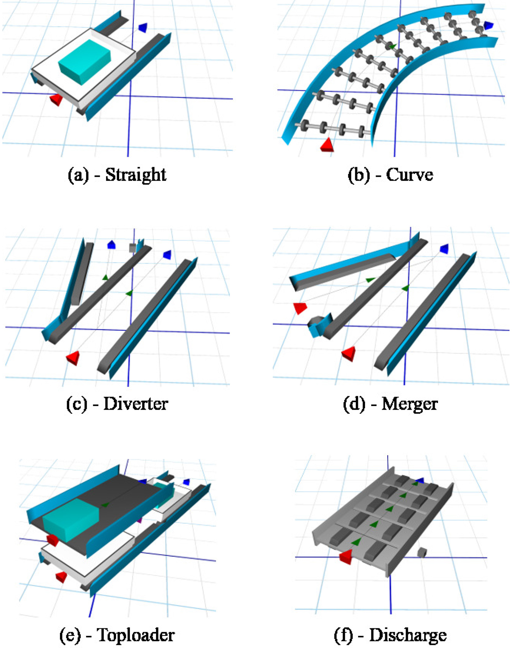

The CrisBag system has some basic elements, as seen in Fig. 1, namely a straight, curve, diverter, merger, toploader and a discharge. The straight and curve elements are, with a routing perspective, functionally the same.

The job of the diverter element is to divert incoming totes if they are supposed to change direction. When using the shortest path approach, the decision on diverting a tote is based on routing tables, possibly overruled by some site-specific routing rules. The job of the merger element is to merge two lines. If totes are waiting on both lines, the merger will toggle on which lines to serve, first allowing a tote from line 1 to pass, then a tote from line 2, etc. The toploader is the element which loads new baggage into totes. The destination of the baggage is not known until it reaches a scanner related to the toploader. Finally, the discharge is an element which tips the baggage out of the tote to deliver it to its destination. It is important to note that the tote stays on the rail, continuing in the system as it is routed towards the toploader to pick up new baggage.

The performance of a BHS is hard to define, but some measures are the average time to delivery and the throughput of totes. It is also an advantage to have a high capacity in the system, as this will help to make the experience for the passengers better by reducing the length of the queue to baggage check in. The capacity is defined as the number of totes which the system can route without the occurrence of deadlocks.

1.2 Related work

1.2.1 Dijkstras shortest path algorithm

In a graph environment, Dijkstras algorithm [12] calculates the path with the lowest cost from every node to all other reachable nodes. If the cost represents the length between nodes, the algorithm finds the shortest path, given that all costs are non-negative. When used in BHSs, the shortest path is stored in routing tables, which for each diverter, states the shortest path to the desired destination. When routing in an environment with a continuous flow and without any congestion, the shortest path is guaranteed to be the fastest route possible. However, this is rarely the case in BHSs, where individual totes can affect the other totes in the system. Therefore, additional rules are often used to dynamically update routing.

1.2.2 Deep reinforcement learning

RL is one of the three main branches of machine learning, namely supervised learning, unsupervised learning and RL. In supervised learning a model is trained using labeled data, whereas in unsupervised learning the model is trained entirely from raw data without any labels or supervision. RL is very different since it uses an agent to learn optimal actions based on experience in an environment. The state of the environment is available to the agent, and it can perform some action to make the environment change its state and possibly release a reward. The goal for RL is to maximize the accumulated reward given by the environment by choosing the best actions.

Q-learning is a model-free, value-based branch of RL. Such methods directly learn a reward function from the state space, without using an explicit transition function or model. This is an advantage when the transitions function becomes more complex to learn than the reward function itself, as it quickly becomes the case in large BHSs. Another advantage with the model-free methods is that they avoid the extra time overhead created by using a model. This does, however, come at the cost of slower convergence.

Value-based methods learns to predict the expected reward for each action, and then chooses its actions according to some policy, usually the greedy policy, choosing the actions which is expected to give the highest reward.

In Q-learning, the environment is treated as a Markov Decision Process, allowing the use of the Bellman Equation [13]. Bellman describes how the discounted sum of future rewards seen in Eq. (1) can be expressed as Eq. (2), where $R_{t}$ is the discounted sum of future rewards at time step $t$ , $r$ is the reward and $\gamma$ is the discount factor.

$\displaystyle R_{t}=\sum_{k=0}^{\infty}\gamma^{k}r_{t+k+1}$ (1) $\displaystyle R_{t}=r_{t+1}+\gamma R_{t+1}$ (2)

The Q-function is shown in Eq. (3), where $Q$ is the policy, $s$ is the state and $a$ is the action. In Q-learning, the Q-function is iteratively updated using the update policy described in Eq. (1.2.2), where $\alpha$ is the learning rate.

$\displaystyle Q(s,a)=E_{\pi}[R_{t}|s_{t}=s,a_{t}=a]$ (3) $\displaystyle Q(s_{t},a_{t})\leftarrow(1-\alpha)\cdot Q(s_{t},a_{t})+$ (4) $\displaystyle\quad\alpha\cdot(r_{t+1}+\gamma\cdot\mathop{\textit{max}}\limits_% {a}Q(s_{t+1},a))$

In its basic form, the Q-function is a table of size $S\times A$ , where $S$ is the number of possible states and $A$ is the number of actions. However, this is not scaleable when the state space becomes large. To overcome this problem, the Q-function can be estimated using a function approximator. This leads to a parameterized Q-function, which is usually updated as in Eq. (5), where $\theta$ is the parameters and $Y_{t}^{Q}$ is the target value.

$\displaystyle\theta_{t+1}=\theta_{t}+\alpha(Y_{t}^{Q}-Q(s_{t},a_{t};\theta_{t}% ))\nabla_{\theta_{t}}Q(s_{t},a_{t};\theta_{t})$ (5)

In [2], they succeed in using a Deep Neural Network (DNN) as the Q-function approximator. They do this by training the DNN, referred to as the online network, on a batch of experience from an experience replay buffer. The target for the online network was the immediate reward added with the expectation of future rewards from the next state determined by an older version of the online network called the target network. This target is defined in Eq. (6), where $\bar{\theta}$ is the parameters of the target network. With a certain interval, the parameters of the online network will overwrite the parameters of the target network, giving the algorithm a new and better target. As the reward $r_{t+1}$ will add new ground truth information to the target, the method will in time converge.

$\displaystyle Y_{t}^{\textit{DQN}}=r_{t+1}+\gamma\mathop{\textit{max}}\limits_% {a}Q(s_{t+1},a;\bar{\theta}_{t})$ (6)

They call the method Deep Q-Network (DQN) and it proves to be a very powerful function approximator, capable of learning how to play different ATARI 2600 games better than humans using only the raw pixel values as input. As Q-learning is an offline learning policy, the training is done on batches of previous experiences. By using the experience replay buffer, it is possible to shuffle the experience, effectively removing the correlation of the temporal connections of consecutive data samples.

The work is extended in [14] with Double DQN, which combines the idea of Double Q-learning [15] with DQN. The idea is to use the online network to determine which action to take and the target network to evaluate the action chosen, as seen in Eq. (1.2.2), where $\overline{\theta}$ is the parameters of the target network and $\theta$ is the parameters of the online network. Doing so decrease overestimation of rewards, which is a problem with DQN.

$\displaystyle Y_{t}^{\textit{DoubleDQN}}\equiv r_{t+1}+$ (7) $\displaystyle\ \gamma Q\left(s_{t+1},\;\mathop{\textit{argmax}}\limits_{a}% \left(Q\left(s_{t+1},\;a;\;\theta_{t}\right)\right),\;\bar{\theta}_{t}\right)\;$

PER is then introduced in [10]. Here it is shown how the error can be used to prioritize the experience gathered in the experience replay buffer. When having a high error, the information of the sample is expected to be high. The probability of sampling a sample from the experience replay buffer is defined in Eq. (8), where $p_{i}=|\delta_{i}|$ , where again $\delta_{i}$ is the error for sample $i$ , and the exponent $\alpha$ determines the influence of prioritization, with $\alpha=0$ describing uniform sampling of the experience replay buffer.

$\displaystyle P(i)=\frac{p_{i}^{\alpha}}{\sum_{k}p_{k}^{\alpha}}$ (8)

As this will change the distribution of used experience, a weighted importance sampling method, seen in Eq. (9), is used by using $w_{i}\delta_{i}$ to update the Q-function instead of just $\delta_{i}$ .

$\displaystyle w_{i}=\left(\frac{1}{N}\cdot\frac{1}{P(i)}\right)^{\beta}$ (9)

This greatly improves both model training time and model performance, as experiences giving rewards are used for training more often.

Finally, Dueling DQN is introduced in [9]. Here, the end of the DNN is split in two where each part is responsible for estimating the value function and the advantage function respectively. This makes sense, as the Q-function consists of these two parts as seen in Eq. (10), where $V(s)$ is the value function, describing the value of the state, i.e. the average expected future reward under the given policy, and $A(s,a)$ is the advantage function, describing the expected additional reward of the immediate next step given the actions.

$\displaystyle Q(s,a)=V(s)+A(s,a)$ (10)

To ensure separation of the two branches of the network architecture, the average advantage is subtracted from the advantage branch, as seen in Eq. (1.2.2). This way, the average reward from the actions will become the responsibility of the value function, allowing the advantage function to only calculate the action specific part of the reward.

$\displaystyle Q(s,a;\theta,\alpha,\beta)=V(s;\theta,\beta)+$ (11) $\displaystyle\quad\left(A(s,a;\theta,\alpha)-\frac{1}{|A|}\Sigma_{a^{\prime}}A% (s,a^{\prime};\theta,\alpha)\right)$

The advantage of using the Dueling DQN architecture is that the value bias is removed from the advantage branch of the network, effectively letting that part of the network learns more precise estimations of the individual actions influence on the expected reward. The Q-function is updated the same way as in Eq. (1.2.2).

Figure 2.

(a) DQN is implemented using a DNN with a single output layer giving a per action estimation of the reward from the state. (b) Dueling DQN use a common DNN stem architecture splitting into two output branches. One to estimate the average reward from the state, V(s), and one to estimate the individual influence of each possible action, A(s,a).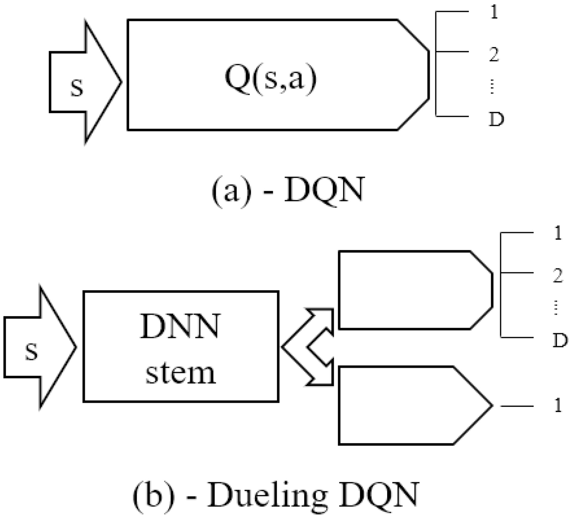

1.2.3 Routing with reinforcement learning

The advantages of using RL as route optimization is the automatic adaption to the environment it is used on. RL should be able to utilize the underlying mechanics of the environment for its own advantage. Using reinforcement learning for routing is not a new idea. Many successful methods have been proposed, however, none which both use the global environment as input to control the entire output and satisfies the context of a BHS with multiple carriers.

In [16], a RL algorithm is used to find good routing policies for intradomain traffic engineering problems. The agent observes a demand matrix and choose a routing strategy to be used for the next epoch. They find that using RL for this task is troublesome, as it takes too long to converge in the training phase. They expect that this result is due to a large output space.

In [17] a Deep RL approach is proposed for solving the Vehicle Routing Problem (VRP). The method consists of using convolutional layers to create an embedding of the input. A Recurrent Neural Network with an attention mechanism is then used on the embedding to create an output sequence. This sequence describes the suggested routing for the carrier vehicle. The method is, according to the authors, flexible and applicable for many different routing problems. The method proves superior to its baselines, including Googles OR-Tools. It is, however, focused on optimizing for single vehicle performance, and does therefore not consider the interaction between multiple vehicles. An issue with methods proposed for the VRP, when considering routing in BHSs, is that they do not consider the cars as individual carriers capable of blocking each other. In this paper, a method capable of routing multiple individual carriers was explored.

In [18], another Deep RL approach is proposed for solving complex online control problems with the example of data flow in data centers. The method splits the problem into two categories, short and long flows, where short flows are small data packages and long flows are large data packages. They adopt a global view on the data center system, controlling all flows when the data packages are in the long flow domain, and use a local view when they are in the slow flow domain. Compared to the BHS domain, the speed dependency is very different, as the BHS is much slower. When routing in the data package routing domain, data can be transmitted to different sources multiple times, and it cannot be blocked or delayed on its way to a new node.

In [19], the Q-routing algorithm, which uses distributed agents to choose directions at each node in a data transportation network, is introduced. It uses RL to make distributed decisions based on local information and messages passed on from its neighboring nodes. It is an online learner, meaning that it learns while routing, making it adaptable to changes in the system. This makes it a viable method for especially data package routing, as bad routing choices is not irreversible and only results in worse performance.

Deep Q-routing [20] is proposed as an extension to the Q-routing algorithm, altering the Q-function to use a DNN as function approximator. It shows that by including information about the current destination, the action history and future destinations, the Q-routing can be improved in regard to both average packet delivery time and convergence time.

1.2.4 Route optimization in baggage handling systems

Route optimization in BHSs has been approached in various ways.

In the work of [21], Model Predictive Control (MPC) is used to find good routing choices for a DCV based system. They present three approaches focusing on delivering a set of DCVs to their respected destination, within a certain time frame. The setup uses a finite horizon, as the environment terminates when all totes have been routed to their destination. Like in [8], the carriers disappear after they have delivered their load. The environment is built up as a graph with nodes and edges, where a node acts as a junction for any number of inputs and outputs. The first approach is to use a centralized MPC, computing entire routes for each bag entering the system. This method achieves good performance; however, it is computationally heavy, making it infeasible to use in real time. The second approach is using a decentralized MPC, where directions are computed locally at each junction in the environment. Compared to the centralized approach, this approach is much faster, but does not achieve as good a performance. The third approach is to use a distributed MPC, which is very similar to the decentralized approach, but with communication between the junctions of the system. This increases the computation time a bit, however it also results in a much better performance. To solve the problem of computation time, a heuristic is applied. From this work, it can be learned that a centralized approach can achieve better routing schemes on the cost of computation time.

Another approach is presented in [22], where software agents are used to decide the routing. Here totes stay in the system after delivering their baggage, making this environment an infinite horizon problem. Performance is measured on the ability to deliver totes within a certain time frame, and on how many rush bags is created. A rush bag is a bag which needs to be delivered by hand because it cannot reach its destination in time on the BHS. Several different agents are used; however, the five most important ones are ToploaderAgents, DivertAgents, MergeAgents, DischargeAgents and a mediator type called RouteAgents. These agents communicate with each other, negotiating about the direction to send totes in. This approach gives a very high performance with good dynamic properties. It is even capable of prioritizing baggage with short time to departure. The communication between agents, however, puts a heavy load on the CPU, making it hard to use in real time systems. The approach is also dependent on a set of manually created schemes, which the agents use depending on what is communicated between them. This work shows that it is possible to achieve better routing schemes when considering the state of the system. It does however come at the cost of a communication overhead and the need for manually specified routing schemes.

In [23], RL is used to route a BHS by aggressively learning which routes not to take. This is inspired from the ant colony routing scheme [24]. It works by using a table-based 1-step Q-learning method with a learning rate of 1.0. This way, when a carrier drives a wrong way, the algorithm removes the action from the possible set of actions from this state, effectively decreasing the search space of the algorithm. This decrease in the search space is important as the table-based method cannot handle large state and action spaces. It does however also induce some problems, as the generality of the model is decreased.

DQN-routing [25] is another extension to Q-routing, also using a DNN as function approximator. It shows that RL can optimize for multiple objectives in a BHS, in this case both for average packet delivery time and for energy consumption. The Q-routing extensions, Deep Q-routing and DQN-routing clearly shows one of the main advantages of using Deep RL, namely that the objective of the model can be changed to fit the need of the user. However, these two methods both use local information to make distributed decisions.

In [8], the strategy from Double DQN [14] is used on a BHS environment implemented with petri nets. Here, a centralized approach is taken, where the information from all elements in the target BHS is used as input, and the output determines the control of all diverters in the BHS. A matrix of size $E\times F$ where $E$ is the number of elements and $F$ is the number of features per element, represents the environment. In the examples, every element has 5 different features: Destination, Occupied, Distance to place, Time in transition and Time in system. The output of the function approximator is bound to be of size $P\times d_{\textit{max}}$ where $P$ is the number of decision point and $d_{\textit{max}}$ is the maximum number of directions to take at any decision point. In this work, the decision points can have any number of output directions. Consecutive straight elements are grouped, and a maximum capacity is enforced. Totes are moved through these grouped elements using the FIFO concept. When totes reach their destination, they are removed. The goal is to route a predefined set of totes to their destination, using as few steps as possible, therefore this work is restrained to a finite horizon problem without a cyclic behavior. The results show that it is possible to get a better performance than dynamically adjusted shortest path, using RL trained with a high load.

2. Method and implementation

From the related work, it can be seen that a general trend is to use distributed decision systems, however in [21], it is shown that using a centralized method is better in terms of performance, but not in terms of speed. Common for the Q-routing method and its extensions [19, 20, 25], is that they rely on local information and messages from neighboring nodes to make distributed decisions.

This paper focus on using Deep RL as a centralized approach to control all diverters in a simulated cyclic BHS environment with an infinite horizon. As the method is centralized, the RL agent is able to use information from the entire BHS to make its decisions. The state of the environment is treated as an image, which is constant in size, making the inference time independent on the load of the system. The performance is measured as the average time to delivery, the average throughput and the number of deadlocks occurring at the specific load.

In this section, a detailed description of the implementation of the method will be given together with details about the Deep RL setup.

2.1 Environment

To train a RL model, an environment is needed. This section will describe how the environment was implemented and how the interface to the environment was structured.

While [8] focused on getting a fixed number of totes from source to destination using as few steps as possible, the goal in this work was instead to get as much baggage collected and delivered as possible. The environment was made to be used for training with an infinite horizon, however, it was set to always stop after a fixed number of steps for each episode to allow for evaluation of the training and to add initial states to the experience replay buffer. Deadlocks would, however, also end the episode.

The environment was implemented in python using two different classes, an Element class and a Tote class. An instance of the Element class was a standard straight (or curve) element. The Element class had four sub-classes, namely; Diverter, Merger, Discharge and Toploader. A subset of the elements was chosen as Discharge elements and Toploader elements, according to the planned environment.

Every element could be assigned an instance of the Tote class. The number of totes were restricted to a maximum of one per element. Every Tote instance was assigned a destination, which could be either a Discharge element or a Toploader element. If the destination was a Discharge element, the tote was loaded with baggage, which had to be delivered to the destination, if the destination was a Toploader element, the tote would be empty and would have to pick up new baggage at the destination.

The environment was initialized with a preset number of totes. These totes were evenly inferred at every Toploader element at every time step, until the environment had reached the required number of totes. The destination for the totes was chosen uniformly by random from the Discharge elements.

To perform a step in the environment, first, all elements containing a tote tried to move the tote forward to the next element. For Diverters, the next element was chosen by the assigned action. A tote could be moved only once per step, and the step algorithm continued until all totes had been moved or blocked by a moved tote. If at some point it was not possible to move any totes, but none were blocked by other moved totes, a local deadlock had appeared. In this work, a local deadlock was allowed. If no totes had been moved during the step, a global deadlock had appeared and a deadlock would be registered. After the movement phase, the algorithm found the totes which had reached their destination. If their destination was a Discharge, the reward was counted up and the totes were directed towards a Toploader. If their destination was a Toploader, they were not given a reward, but directly directed towards a Discharge, simulating that new baggage was inferred. If a deadlock was registered, the environment was reset.

2.1.1 Observation

To be able to observe the state of the environment, a RL agent must get some description of the state. This was given through an observation, which was returned by the environment after every step. The observation space of this environment was given as an $E\times F$ matrix with $E$ being the number of elements in the environment and $F$ being the number of features. This way, the agent receive information about the entire BHS, as opposed to the approach from [19, 20, 25], where local information around multiple agents are used, combined with information from their neighboring nodes. The elements are ordered mainly by their occurrence in the environment as seen by the element IDs in Figs 5–7. However, as diverters create discontinuities, other measures, such as the length of connected paths and the similarity of element sections, also contribute to the ordering.

In this implementation, only a single feature is used, an integer representation of the destination for the tote occupying the element. If there was no tote present, the value would be 0. If a tote is present and had a destination which was a Discharge, the value would be the index of that Discharge. This index would always be in the range of 1 to the number of Discharge elements. If a tote was present and had a destination which was a Toploader, the value would be the index of that Toploader. The index would be found in the same way, but described as a negative number, i.e. ranging from $-$ 1 to negative the number of Toploader elements. This way, the data was approximated towards being zero-centered. Zero-centered data can be an advantage when training DNNs, as this reduce the bias term from the data, making the learning task easier. An interesting experiment would be to use one-hot encoding of the destinations instead, as this would remove the numerical dependencies. This is, however, not considered in this work, and therefore left for future research.

The size of the observation space can be approximated using Eq. (12) where $N_{T}$ is the number of Toploaders in the environment. However, since the rules of the environment did not differentiate between different Toploader elements when filling baggage into the tote, these could be merged into one, leading to Eq. (13), which is the equation used in this paper to estimate the observation size. This equation does not take illegal positions into consideration. An illegal position would for instance be a tote with a destination of the Discharge element, which it had just passed.

$\displaystyle\text{Observation size}_{\text{Max}}\equiv(D+N_{T}+1)^{E}$ (12) $\displaystyle\textit{Observation size}\equiv(D+2)^{E}$ (13)

2.1.2 Action

To be able to affect the environment, an RL agent must perform actions. These actions must follow the guidelines set by the environment. In this environment, the action space had to be a vector with a length equal to the number of Diverter elements $D$ in the environment. The values of the vector could be either 0 (let pass) or 1 (divert).

2.1.3 Reward

To be able to learn, an agent needs to receive rewards. Rewards can be either positive or negative. Actions leading to positive rewards will be reinforced, while actions leading to negative rewards will be diminished. Another way to manipulate with the learning is to end the episode before time. If the agent always gets negative rewards, such as a negative reward per step used, the agent will search for ways to end the episode quickly, as seen in [8]. However, if the environment does not give negative rewards, and if the environment has an infinite horizon, the agent will always try to find a way to avoid early termination.

In this environment, a reward of $+$ 1 was given by the environment every time a tote reached its destination given that the destination was a Discharge element. This led to the agent only receiving positive rewards, and therefore, the early stopping inferred by a deadlock was expected to be avoided by the agent.

2.2 Deep reinforcement learning setup

The Deep RL model was designed with inspiration from the Dueling DQN architecture [9] with PER [10]. Any other model-free, value-based RL method might also be used, however, the Dueling DQN architecture was chosen to isolate the advantage of each action to each Diverter element and to separate the general value of the state from the actions taken. Together with PER, this was an important part of the implementation, since the actions often would not have any impact, as they only affected the environment when a tote was present.

The environment marked the episode as done, only if the environment encountered a global deadlock. The target for the Q-function was formulated as Eq. (14). This detached the horizon from the learning, while still allowing the model to learn how to avoid deadlock situations.

$\displaystyle Y_{t}=\left\{\begin{array}[]{ll}r_{t+1}&\textit{if deadlock}\\ r_{t+1}+Q_{t+1}&\textit{otherwise}\end{array}\right.$ (14)

2.2.1 Deep neural network architecture

The architecture was based on the work in [8], where a convolutional neural network (CNN) is used to capture relevant features from the observation. The reason why a CNN is a good choice for this type of problem is because it can utilize the spatial connectivity between the elements in the state vector. The architecture also allows for multiple features in the input without implying a spatial relation between them.

In the BHS environment, totes are often in positions, where actions will not change the expected reward. Therefore, the state will imply an expected future reward independent on the individual actions proposed by the RL agent. To let the DNN capture this information, the Dueling DQN architecture was used, as seen in Fig. 3.

Figure 3.

DNN architecture. E was the total number of Element instances in the environment while D was the number of Diverter elements in the environments. After each layer, a ReLU was used as activation function.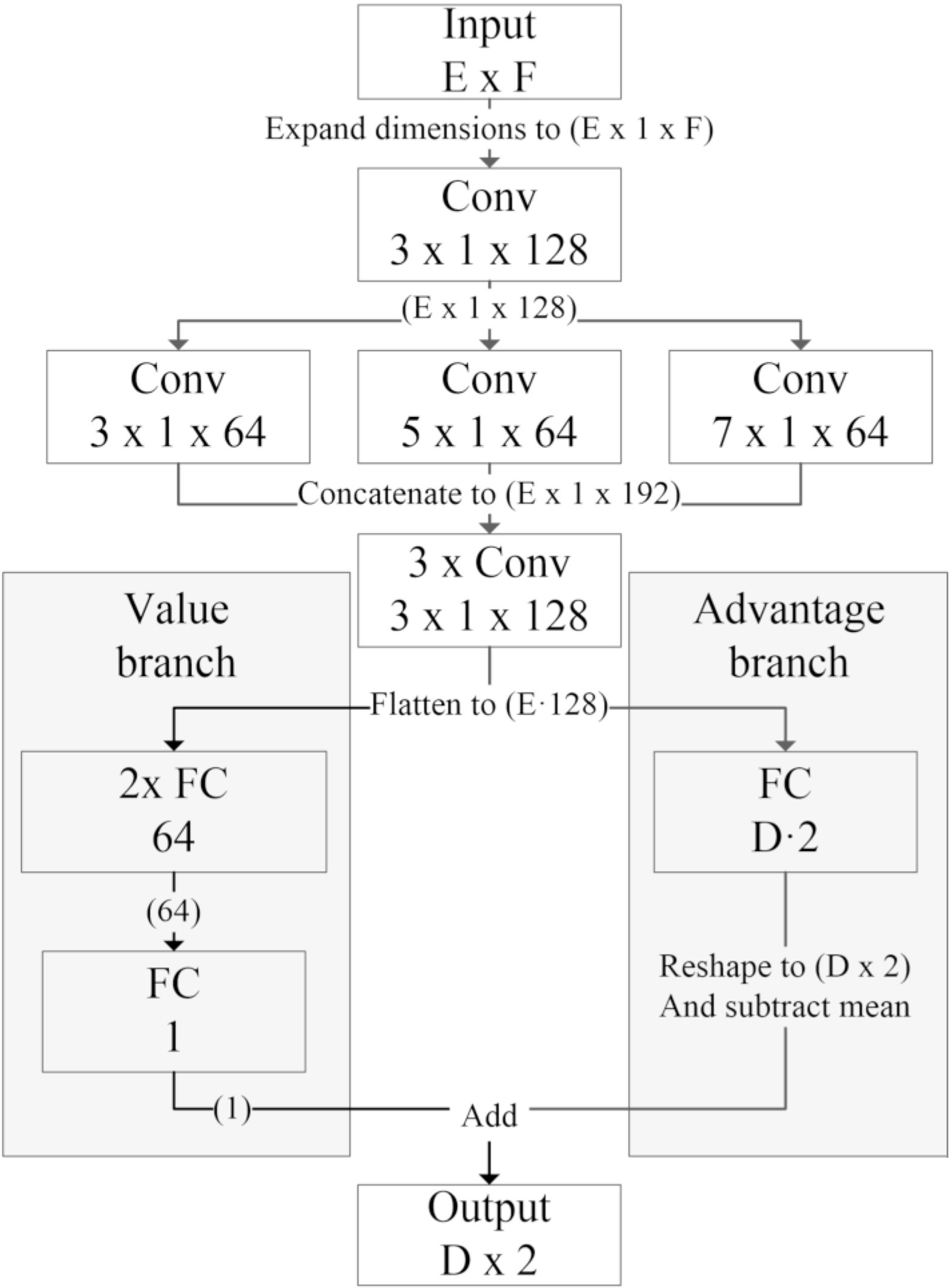

The input was fed through a stem architecture where information about the order of the elements were kept. The stem consisted of a convolutional layer, followed by three parallel convolutional layers of different size and ended with three sequential convolutional layers. This way, local low-level features were captured at different scales and by different hierarchical levels. Then, as the Dueling DQN architecture describes, the advantage and value estimations were separated. Here, the value branch was chosen to be implemented using three consecutive fully connected layers. The advantage branch was kept the same as the original architecture from [8].

The output of the DNN was organized as a $D\times 2$ matrix, where each row described the total expected future reward for the actions of a Diverter element.

The loss was then found using the Huber loss on the mean absolute error as described in Eq. (15).

$\displaystyle L=L_{\delta}\left(E\left(\left|Q(s_{t},{\bm{a}})-\!\!\phantom{% \frac{r_{t+1}}{D}}\right.\right.\right.\left.\left.\left.\left(\gamma Q^{% \prime}(s_{t+1},{\bm{a}})+\frac{r_{t+1}}{D}\right)\right|\right),\delta=1\right)$ (15)

Where

$\displaystyle Q^{\prime}(s_{t+1},{\bm{a}})=$ (16) $\displaystyle\quad Q(s_{t+1},\mathop{\textit{argmax}}\limits_{a}(Q(s_{t+1},{% \bm{a}};\theta);\overline{\theta})$

An overview of how this concept of using a Deep RL agent to globally control a BHS is integrated, can be seen in Fig. 4.

Figure 4.

The general concept of using a Deep RL agent to globally control a BHS with multiple actions.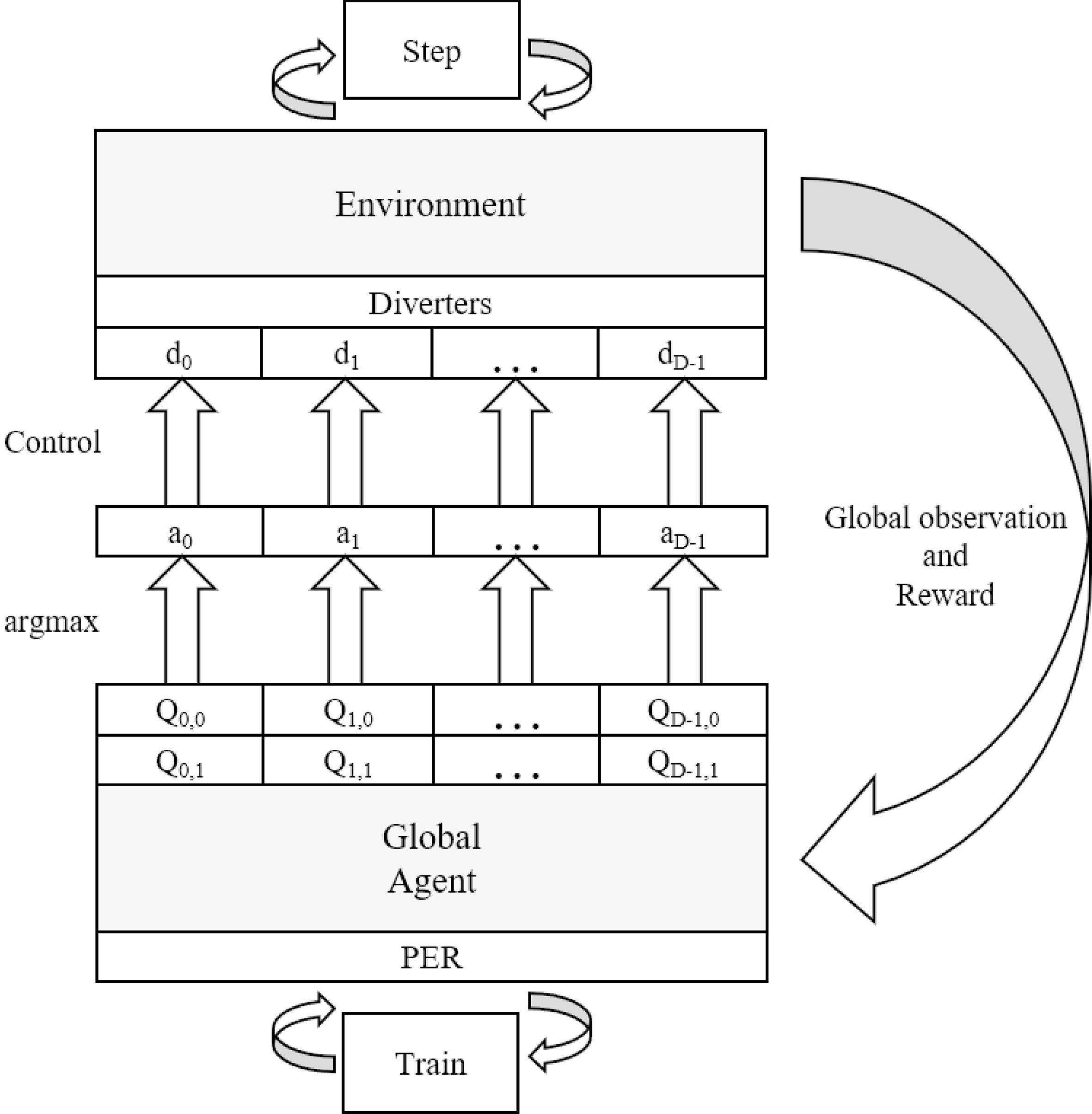

2.3 The shortest path

To be able to compare the performance of the RL model, two routing algorithms have been used, namely the Dijkstras shortest path algorithm [12], referred to as the Static Shortest Path (SSP) and a dynamically updated version of the shortest path algorithm, referred to as the Dynamic Shortest Path (DSP). DSP is very similar, in terms of functionality, to the vanilla routing system in real BHSs, without site-specific routing rules.

SSP was calculated once and used to make a routing table, which Diverter elements then used to route totes to their destination. This method was fairly simple and computationally fast to use at run time since it only required a table lookup. To find the shortest path, the cost of each route was required. In this implementation, all elements on the route was given a cost of 1. This method, however, did not consider other totes in the system when choosing a direction. Therefore, it could lead totes directly into a congested path, which could result in a deadlock.

DSP was initiated the same way as SSP, however, when a congestion was registered, the routing table was recalculated. A congestion was defined as when all elements on the output of a Diverter or Merger element, until the next Diverter or Merger element, were occupied with a tote. When this happened, the cost of these elements was increased to a cost of 100, making the route very expensive compared to alternative routes. When the congestion disappeared, the cost of the elements was changed back to 1 and the routing table was recalculated. This way, the routing had a better chance of avoiding deadlocks, without having to recalculate the routing table at every time step. However, at high loads, DSP required the shortest path to be recalculated often, which was a time-consuming process.

As an add-on, a naive Deadlock Avoidance (DLA) policy was also applied to DSP. This policy worked by forcing totes to avoid entering a fully congested path in the BHS. This method did not guarantee the avoidance of deadlocks; however, it did lower the risk of deadlocks even further. It could however come at the cost of sending totes in a direction, where they would need to take large detours just to reappear at the same diverter again later. This method is referred to as DSPdla.

3. Experiments

3.1 Environments

To test the proposed method, three environments of different size and complexity was used. Environment 1, seen in Fig. 5, was the smallest and simplest of the three environments. It contained only a single Diverter element, giving the agent a single action possibility. The environment consisted of 34 elements, which, by using Eq. (13) lead to a state space of $(5+2)^{34}=5.41\times 10^{28}$ . Since a congestion could only appear at Toploader elements and Merger elements, Environment 1 only had two possible origins of congestion. When the number of totes in the environment was below 18, which was the shortest connected route, deadlocks could not appear. The tricky part of this environment is that the controller only has information about totes at element 0, 1 and 2 before it needs to make a decision about which direction it should send the tote on element 2 in. It is therefore hard to make complex strategies on how to route totes with the destination Discharge 20.

Figure 5.

Environment 1. A simple environment containing 34 elements with only 1 diverter and 5 discharges.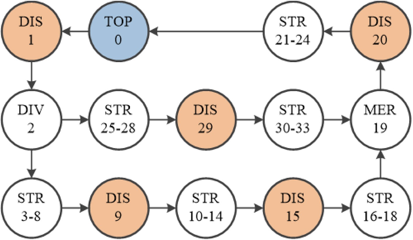

Environment 2, seen in Fig. 6, contained 7 Diverter elements, and had no symmetry, making it a much more complex environment than Environment 1. The number of elements was 101, making it almost three times larger than Environment 1, and it had 7 Discharge elements, which gave it an observation space with a size of $(7+2)^{101}=2.39\times 10^{96}$ . This environment introduced three return paths, which allowed the controller to send a tote back in the system if for instance it had missed its Discharge element. In real BHSs, the discharges are often placed next to each other in groups at each terminal. However, some systems are only subparts of larger systems, in which case, the discharges unloads baggage to other conveyors. This type of system is often more chaotic, which was what Environment 2 simulated.

Figure 6.

Environment 2. A complex environment containing 101 elements with 7 diverters, 7 discharges, no symmetry and 3 return paths.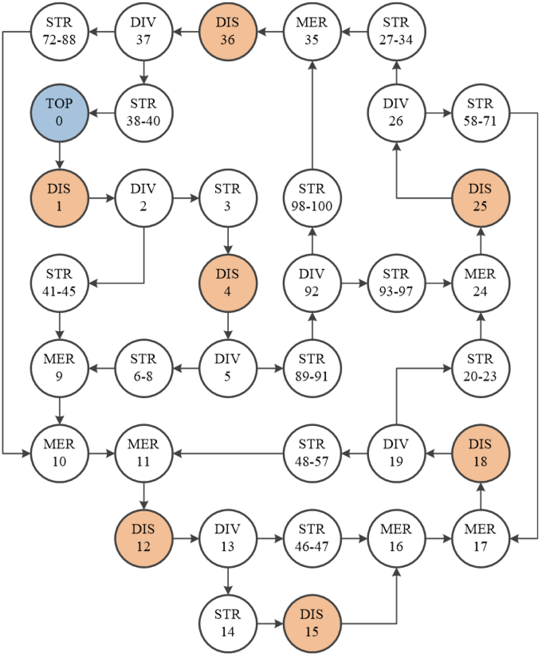

Environment 3, seen in Fig. 7 was the largest of the three environments, it consisted of 265 elements and therefore had an observation space of $\left(2+2\right)^{265}=3.51\times 10^{159}$ . This environment was symmetrical, and allowed totes to switch between the left and right part three times during the flow. This environment was therefore, despite its 10 diverters, a less complex environment to control than Environment 2. The design was a small version of the design used in [21], which was considered to be a design very similar to real world designs of small BHSs.

Figure 7.

Environment 3 contains 265 elements.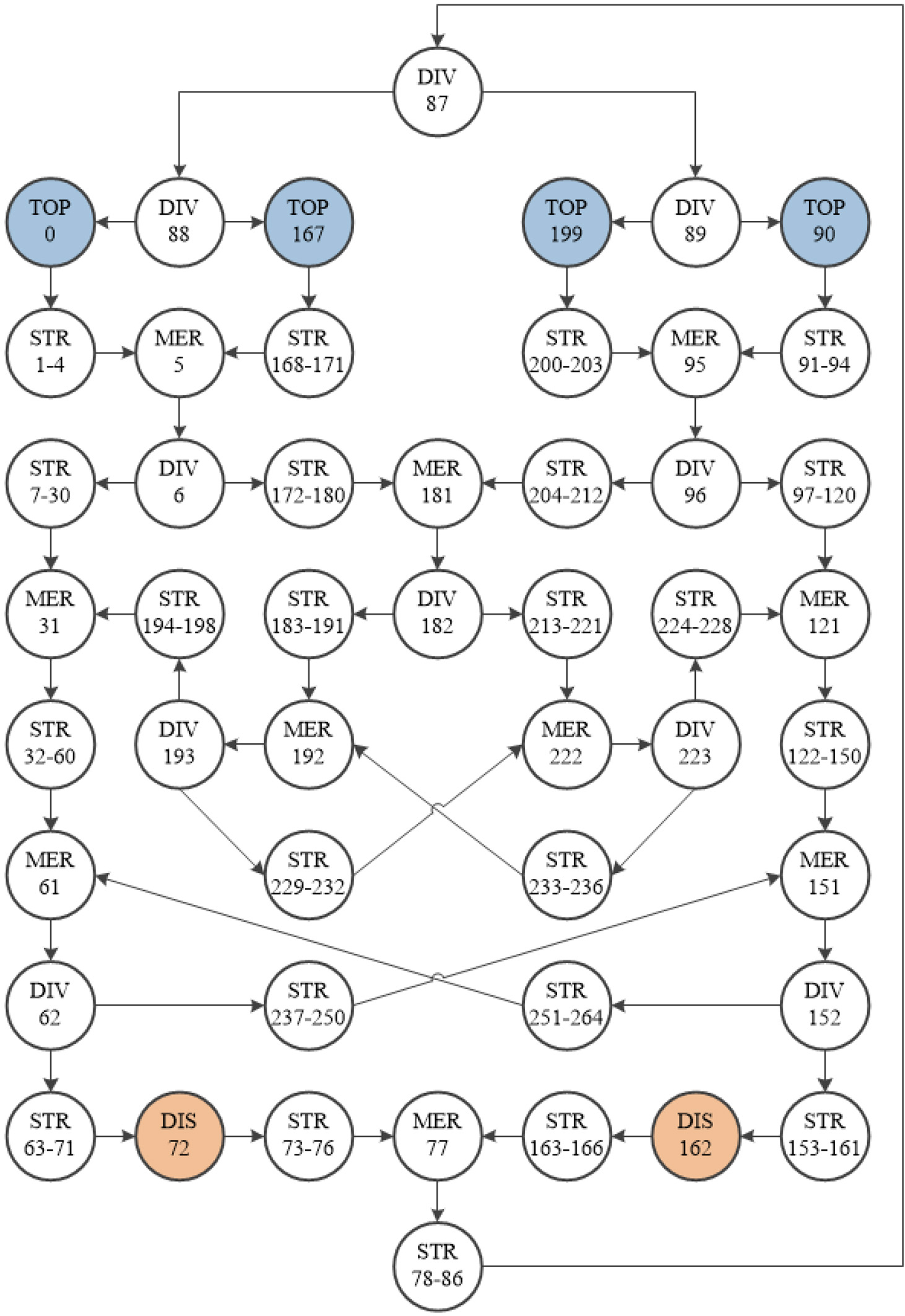

General for all three environments was that they were small, compared to real world BHSs. This was a limitation caused by high simulation time when simulating larger systems. Real systems are often in the range of 1000–10000 elements.

3.2 Training

From the work in [8], it is found that when training a RL model on an environment, the number of inducted totes is important. It is also found that the system learns the most when a high number of totes is inducted. This was, however, not guaranteed to be true for the cyclic environments used in this work. Therefore, models were trained using five different loads, namely 10%, 30%, 50%, 70% and 90%. The load was defined as the number of totes used, divided by the number of elements in the environment. Furthermore, a model was trained using the same setup, but with a random load in the range of 1–100%, randomly re-selected at each reset.

The models were trained with backpropagation using the RMSprop optimizer using a batch size of 32, as suggested by [25]. The models were trained in two iterations of 10 million steps, using a learning rate of 1e-3 and 1e-4 respectively. The exploration was set to be 50% in the beginning of each iteration, and linearly decrease to 2% after 1 million steps.

Lastly another model with two extra fully connected layers of size 64 in the value branch was trained. This model was also trained with backpropagation using the RMSprop optimizer using a batch size of 32, but only for 10 million steps, with an exponentially decaying learning rate starting at 1e-3 with a decay of 0.96. The exploration was the same as with the other models.

For both training setups, a PER buffer with a size of 100000 have been used with $\alpha=$ 0.6 and $\beta=$ 0.4. We chose the buffer size to be large, to allow the model to learn from past experience where exploration was higher, despite it being more focused on exploitation for new experience gathering.

Environments 1 and 2 were reset every 2000 steps, and Environment 3 was reset every 5000 steps. This was done to learn to route both in initial and saturated states of the environments. A concern could be if this would limit the infinite horizon concept of the training process, but as seen in Eq. (14), only deadlocks would introduce a terminate-state, therefore, this was not an issue.

The training was performed on an NVIDIA TITAN X Pascal GPU, using TensorFlow v1.8.0.

3.3 Tests

To test the performance of the trained models, they were first compared to each other to find a suitable competitor to the three shortest path methods, SSP, DSP and DSPdla.

When testing, the performance was measured by the number of delivered bags within an episode length of 200 steps for Environments 1 and 2 and 500 steps for Environment 3. This step-limit was enforced to be able to compare the performance of the different routing strategies equally. The step-limit was chosen to be large enough for the environment to be filled with the expected load and for it to run with this load for approximately an equal number of steps or more. After each episode, the environment was reset. The models were tested on all loads from 1 tote to 100% load, by increasing the number of totes by one for each test. Each test was performed 100 times with a new seed for the random generator, choosing the destinations of the totes. The same seed was used for the competitors at the same load and iteration. The number of deadlock occurrences in the 100 tests was also registered as a measure of performance for that load.

3.4 Results and discussion

In this section, the RL models will be referred to as RL followed by the percentage of load they were trained with. I.e., a model trained with 50% load will be referred to as RL50. The two models trained with a random load is referred to as RLR and RLR+, with RLR+ being the model trained with an exponentially decaying learning rate.

When comparing the reward of the five RL models trained with specific loads, there was a general trend towards each model having a global maximum approximately around the load where it was trained, which is not surprising. It was, however, surprising to see that the model trained with the same setup, but with a random uniform distribution of loads, RLR, was superior to the other models at almost every load as seen in Fig. 8. This contradicted the experience gained in [8], and was expected to be caused by the more realistic implementation of the environments, and the cyclic behavior with infinite horizon.

Figure 8.

Reward of RL models for all environments. In all environments, the models trained on a specific load, tended to work well around that specific load. Exceptions did occur, such as the RL10 in Environments 1 and 3, which seemed to find a policy applicable to higher loads as well. RLR achieved the best policy for almost all loads, making it superior to the other RL models.

From the results of comparing RLR, RLR+, SSP, DSP and DSPdla with each other, Fig. 9, it could be seen that both RLR and RLR+ generally avoided deadlocks up until a higher load than both SSP and DSP. DSPdla was a naive approach to avoid deadlocks, forcing the environment to route totes in a different direction than a full line. This approach proved useful in the simple Environment 1, however as it could be at the cost of sending totes an extra round in the system, without need, RLR and RLR+ was able to score higher points between 70 and 85% load. In Environments 2 and 3, RLR and RLR+ clearly had an advantage over the competitors when the load got high.

Figure 9.

A comparison between RLR, RLR+, SSP, DSP and DSPdla showed that in all environments, the RLR and RLR+ models learned to handle high loads in the system better than SSP, DSP. DSPdla did best in Environment 1, however, it was outperformed in Environments 2 and 3.

Comparing RLR with RLR+ it could be seen that for Environments 1 and 3, RLR+ was better at all points, but in Environment 2, RLR was best. This could be a consequence of the complexity of the environments, as Environments 1 and 3 was of lower complexity than Environment 2. Therefore, it might be that the number of steps required to learn how to effectively route in Environment 2 was higher than for Environments 1 and 3. Even though Environment 3 had a larger observation space, it was symmetric and without return paths before the destinations, making it easier to control.

As the load increases, the dynamic SP algorithms needs to recalculate more often, which makes them very inefficient for large environments. The RLR+ model is measured to make inference in 4–6 ms. for all three environments. As this time does not change when the load increases, the method can be considered to be applicable for real time systems in regards of speed. However, as the size of the environment increases, so does the simulation time and observation size, which is a problem for the Deep RL approach in terms of training and test time.

The expectation about using RL for routing was that it should be able to find the underlying mechanisms of the environment. This was somewhat the case, however since the shortest path methods was better at low loads, RLR was probably not trained well enough for this area. This could have been a classic exploration/exploitation issue, where the model got stuck in a local optimum, where it had generalized to higher loads.

The results of this paper do not give reason to think that RL models are not capable of routing in small BHSs, however future work should explore the scalability of the method to larger systems. Furthermore, it would be interesting to explore the performance with a more realistic distribution of destinations. Often baggage for a certain destination will arrive simultaneously, which would give a local increase of the load on the routes leading to that destination. This might be an advantage for the RL model, compared to the shortest path approaches.

Another interesting thing to investigate further would be the mix of using shortest path approaches together with the Deep RL approach. The shortest path approaches are very effective with low loads, both in regards of computation time, as it is just a look up, and in regards of throughput, as less congestion appear at low loads. The Deep RL approach on the other hand is capable of handling high loads by using a general Q-function to estimate the actions with a computation time independent on the load.

Yet another interesting thing to explore, is the notion of destination time frames, i.e., the time frame in which the baggage needs to arrive at their discharge. This greatly increases the difficulty of the problem; however, it also makes it much more applicable to real systems.

4. Conclusion

This paper showed that by training a centralized, multi action Deep RL model with the model-free, value-based Dueling DQN method with PER, it was possible to route totes in cyclic BHS environments.

The RL models trained with a random and uniform distribution of loads performed best, which contradicts the experience from [8], where a high number of totes were superior to the random number of totes. This change is expected to be caused by the cyclic behavior of the environments in this paper.

Three environments of different size and complexity were tested.

Among the Deep RL models, RLR+ was best in the simple Environments 1 and 3, while in the more complex Environment 2, RLR was best. This was expected to be a consequence of the extra exploration used in the training of RLR.

When comparing RLR and RLR+ to the SP methods SSP, DSP and DSPdla, there was a general trend of the SP methods to be best at low loads. However, when the load increased, the RLR and RLR+ models were superior, as they avoided deadlocks up until a much higher load.

As the inference time of the Deep RL method does not change as the load increases, as opposed to the dynamic SP methods, it is a viable option to use when the environments have a high load. It is however not yet scalable to real size BHSs, as the simulation time makes the training and test time infeasible with the current implementation.

Footnotes

Acknowledgments

For this work, guidance and materials have been provided by BEUMER Group. This work is partly funded by the Innovation Fund Denmark (IFD) under File No. 8053-00040B.

References

ICAO. Annual Report 2017 – Presentation of 2017 Air Transport Statistical Results; 2018. Available from: https//www.icao.int/annual-report-2017/Pages/the-world-of-air-transport-in-2017-statistical-results.aspx

Mnih

Kavukcuoglu

Silver

Graves

Antonoglou

Wierstra

, et al. Playing Atari with Deep Reinforcement Learning. 2013 December.

Silver

Huang

Maddison

Guez

Sifre

van den Driessche

, et al. Mastering the game of Go with deep neural networks and tree search. Nature. 2016 January; 529(7587): 484-489.

Silver

Schrittwieser

Simonyan

Antonoglou

Huang

Guez

, et al. Mastering the game of Go without human knowledge. Nature. 2017 October; 550(7676): 354-359.

Mnih

Kavukcuoglu

Silver

Rusu

Veness

Bellemare

, et al. Human-level control through deep reinforcement learning. Nature. 2015 February; 518: 529.

Vinyals

Babuschkin

Chung

Mathieu

Jaderberg

Czarnecki

, et al., AlphaStar: Mastering the Real-Time Strategy Game StarCraft II; 2019. Available from: https://deepmind.com/blog/article/alphastar-mastering-real-time-strategy-game-starcraft-ii.

Zhang

Leitner

Milford

Upcroft

Corke

. Towards Vision-Based Deep Reinforcement Learning for Robotic Motion Control. 2015 November.

Sørensen

Nielsen

Karstoft

. Deep Reinforcement Learning for Route Optimization in Baggage Handling Systems. In: Yurish

, editor. Proceedings of the 1st Interna-tional Conference on Advances in Signal Processing and Artificial Intelligence. International Frequency Sensor Association Publishing; 2019. p. 29-33.

Wang

Schaul

Hessel

van Hasselt

Lanctot

de Freitas

. Dueling Network Architectures for Deep Reinforcement Learning. 2015 November.

10.

Schaul

Quan

Antonoglou

Silver

. Prioritized Experience Replay. 2015 November.

11.

Baggage handling with container conveying system | BEUMER Group; 2019. Available from: https://www.beumergroup.com/en/products/airport-baggage-handling-systems/high-speed-transportation-systems/crisbagr.

12.

Dijkstra

. A note on two problems in connexion with graphs. Numer Math. 1959 December; 1(1): 269-271.

13.

Bellman Equation. In: Sammut

Webb

, editors. Encyclopedia of Machine Learning. Boston, MA: Springer US; 2010; p. 97. Available from: 10.1007/978-0-387-30164-8_71.

14.

Hasselt

Guez

Silver

. Deep Reinforcement Learning with Double Q-Learning. In: Thirtieth {AAAI} Conference on Artificial Intelligence ({AAAI-16}). aaai.org; 2016. p. 2094-2100.

15.

Hasselt

. Lafferty

Williams

CKI

Shawe-Taylor

Zemel

Culotta

, editors. Double Q-learning. Curran Associates, Inc.; 2010.

16.

Valadarsky

Schapira

Shahaf

, et al. A machine learning approach to routing. arXiv preprint arXiv. 2017.

17.

Nazari

Oroojlooy

Snyder

Takac

. Bengio

Wallach

Larochelle

Grauman

Cesa-Bianchi

Garnett

, editors. Reinforcement Learning for Solving the Vehicle Routing Problem. Curran Associates, Inc., 2018.

18.

Chen

Lingys

Chen

Liu

. AuTO: Scaling Deep Reinforcement Learning for Datacenter. In: {SIGCOMM} ’18; August 20-25, 2018, Budapest, Hungary. p. 191-205. Available from: 10.1145/3230543.3230551.

19.

Boyan

Littman

. Cowan

Tesauro

Alspector

, editors. Packet Routing in Dynamically Changing Networks: A Reinforcement Learning Approach. Morgan-Kaufmann, 1994.

20.

You

Feng

Zhao

. Toward Packet Routing with Fully-distributed Multi-agent Deep Reinforcement Learning. 2019 May.

21.

Tarau

Schutter

Hellendoorn

. Model-Based Control for Route Choice in Automated Baggage Handling Systems. IEEE Trans Syst Man Cybern C Appl Rev. 2010 May; 40(3): 341-351.

22.

Hallenborg

Risager

. DECIDE: Agents Controlling a BHS of an airport hub. Journal of Automation, Mobile Robotics & Intelligent Systems. 2007; 6; 1(2): 50-54.

23.

Johnstone

Creighton

Nahavandi

. Status-based Routing in Baggage Handling Systems: Searching Verses Learning. IEEE Trans Syst Man Cybern C Appl Rev. 2010 March; 40(2): 189-200.

24.

Cong

Schutter

Babuška

. Ant Colony Routing algorithm for freeway networks. Transp Res Part C: Emerg Technol. 2013 December; 37: 1-19.

25.

Mukhutdinov

Filchenkov

Shalyto

Vyatkin

. Multi-agent deep learning for simultaneous optimization for time and energy in distributed routing system. Future Gener Comput Syst. 2019 May; 94: 587-600.