Learning ensembles of priority rules for online scheduling by hybrid evolutionary algorithms

Abstract

This paper studies the computation of ensembles of priority rules for the One Machine Scheduling Problem with variable capacity and total tardiness minimization. Concretely, we address the problem of building optimal ensembles of priority rules, starting from a pool of rules evolved by a Genetic Programming approach. Building on earlier work, we propose a number of new algorithms. These include an iterated greedy search method, a local search algorithm and a memetic algorithm. Experimental results show the potential of the proposed approaches.

Keywords

Online scheduling one machine scheduling hyper-heuristic priority rules ensemble learning maximum coverage problem

1. Introduction

This paper tackles the one machine scheduling problem with variable capacity denoted $(1,\textit{Cap(t)}||\sum T_{i})$ in the conventional ( $\alpha|\beta|\gamma$ ) notation proposed in [1]. In this problem, a number of jobs must be scheduled on a single machine, whose capacity varies over time, with the objective of minimizing the total tardiness objective function ( $\sum T_{i}$ ). This problem arose from the Electric Vehicle Charging Scheduling (EVCS) problem confronted in [2]. Indeed, solving this problem requires solving a number of instances of the $(1,\textit{Cap(t)}||\sum T_{i})$ problem quickly, in an online fashion.

Given the tight time requirements of online scheduling, priority rules are of common use in that setting. A priority rule is an expression that assign a priority to each candidate job to be scheduled at a given time, and so it can be exploited by efficient greedy algorithms. Such algorithms will indeed provide high quality schedules only if the guiding priority rules capture relevant problem knowledge. As an example, in [2] the $(1,\textit{Cap(t)}||\sum T_{i})$ problem is solved by means of the Apparent Tardiness Cost(ATC) priority rule. Priority rules can be defined manually by experts on the problem domain, as it is the case of the ATC rule [3], although it is clear that automatic methods could capture some characteristics of the scheduling problem that are not clear to human experts. For this purpose, approaches as Genetic Programming (GP) are a suitable choice, as they have been in other contexts as image filtering [4, 5] or association rules [6].

In this respect, several authors have adopted the classic GP paradigm proposed by Koza in [7] for learning rules for scheduling problems. These include job shop [8, 9, 10], single machine [11, 12], unrelated parallel machines [13] or resource constrained project scheduling problems [14, 15], among others. Other approaches have emerged such as cartesian genetic programming [16, 17], single node genetic programming island model [18] or hybrid genetic programming [19]. Burke et al. taxonomy [20] classifies these approaches as heuristic generation approaches; more specifically these algorithms are named genetic programming based hyper-heuristics. Besides, data mining alternatives as those proposed in [21, 22, 23] could be exploited to evolve priority rules as well.

In any case, the general idea is to use a set of training instances of the specific problem from which the GP approach conducts a learning process. As in any other machine learning context, these rules must then be evaluated on a number of unseen instances, i.e., a test set. The use of approaches as GP presents two main drawbacks: it is time consuming and, at the same time, it is highly stochastic, so the obtained rules from two independent runs are usually rather different.

As it may be expected, a single rule, even being very effective on average at solving a large set of instances, may not be good for a number of them. For this reason, a number of research works have been focused on calculating sets of rules (ensembles) that collaboratively solve the problem.

The use of ensembles has been considered in some domains, as for example financial risk prediction [24]. Furthermore, in scheduling domains ensembles have been explored in different ways. For example, in [9] Hart and Sim propose a GP approach to obtain a set of rules that are applied in turn to schedule a single operation. This approach was adopted by Park et al. in [25] to analyze four popular combination schemes to solve dynamic job shop scheduling problems. The combination schemes included majority voting, linear combination, weighted majority voting and weighted linear combination. A survey, including these and other schemes, was presented in [26]. Generally, the results showed that the linear combination scheme performs better compared to the other approaches. Durasevic and Jakobovic [27] studied several ensemble learning algorithms for the dynamic scheduling problem with unrelated machines. These methods are simple ensemble combination, BagGP [28], BoostGP [29] and cooperative coevolution. The authors concluded that the best approach was simple ensemble combination. So, in [30] they extended the work presented in [27], focusing on simple ensemble combination. One common feature of these ensemble methods is that all of them exploit the ensemble to produce a single rule following two main approaches: sum and vote. As stated in [27], in the first one the priority values of all rules are summed up to get a priority value, while the second one determines the job receiving the largest number of votes.

In this paper, we follow an alternative approach. Given the short time required to compute a solution to the instances of the $(1,\textit{Cap(t)}||\sum T_{i})$ problem generated when solving the EVCS problem [2], we propose to use a set of priority rules in parallel to obtain a number of solutions, being the best of them the solution produced by the ensemble. Our working hypothesis is that if these rules are specialized on different instances of a representative training set, there will be a high chance that some of them produce a good solution for an unseen instance.

The approach proposed herein starts from a large set of rules produced by GP [12] from a given training set in a number of runs. Due to the stochastic nature of GP, one may expect that this set will include quite different rules. So, the objective is to come up with an ensemble covering all the instances in the training set, i.e., such that for each training instance at least one rule in the ensemble produces a good solution. This problem is termed Optimal Ensemble of Priority Rules Problem (OEPRP) herein. As we will see, the Maximum Coverage Problem (MCP) can be reduced to OEPRP, so this problem is NP-hard and some algorithms for MCP may be adapted to OEPRP.

Earlier work [31] proposed a genetic algorithm for solving the OEPRP. In this paper we extend this work and propose a number of solving methods, namely an iterated greedy algorithm adapted from a classical approach for MCP, a local search algorithm specifically designed for the OEPRP and hybrid algorithms that combine local search with the greedy algorithm and with the genetic algorithm, resulting in a memetic algorithm.

We conducted an experimental study, comparing the evolved ensembles to the best online and offline methods in the literature to solve the $(1,\textit{Cap(t)}||\sum T_{i})$ problem. As far as we know, the best performing methods are a schedule builder guided by the priority rules evolved by GP in [12] and the memetic algorithm proposed in [32]. The results show that the solutions obtained from the evolved ensembles are better than those produced by the best rules obtained in [12] and that these solutions are actually close to those obtained offline in [32].

The remainder of the paper is organized as follows. In the next section we give the formal definition and the solving method used for the $(1,\textit{Cap(t)}||\sum T_{i})$ problem online, which consists of two main components: schedule builder and priority rules. Besides, we describe the results from previous approaches. In Section 3 we present the problem of calculating the optimal ensemble of priority rules (OEPRP) and the proposed solving methods. Next, in Section 4, we report the results from the experimental study. Finally, in Section 5, we summarize the main conclusions and outline some lines for future research.

2. The One Machine Scheduling problem with Variable Capacity

In this section we formally introduce the One Machine Scheduling problem with Variable Capacity and Total Tardiness minimization, $(1,\textit{Cap(t)}||\sum T_{i})$ , and review the current solving methods.

2.1 Problem definition

The $(1,\textit{Cap(t)}||\sum T_{i})$ problem may be defined as follows. We are given a set of $n$ jobs $\{1,\ldots,n\}$ , all available at time $t=0$ , which have to be scheduled on a machine whose capacity varies over time, such that $\textit{Cap(t)}\geqslant 0$ , for all $t\geqslant 0,$ is the capacity of the machine in the interval $[t,t+1)$ . Job $i$ has duration $p_{i}$ and due date $d_{i}$ . The goal is to assign starting times $st_{i},1\leqslant i\leqslant n$ to the jobs on the machine such that the following constraints are satisfied:

At any time $t\geqslant 0$ the number of jobs that are processed in parallel on the machine, $X(t)$ , cannot exceed the capacity of the machine, i.e.,

$\displaystyle X(t)\leqslant\textit{Cap(t)}.$ (1)

The processing of jobs on the machine cannot be preempted, i.e.,

$\displaystyle C_{i}=st_{i}+p_{i},$ (2)

where $C_{i}$ is the completion time of job $i$ .

The objective function is the total tardiness, defined as:

$\displaystyle\sum_{i=1,\dots,n}\max(0,C_{i}-d_{i})$ (3)

which must be minimized.

Figure 1 shows a schedule for a problem with 7 jobs; the capacity of the machine is 2 at $t=$ 0, then it varies non-decreasingly up to 5 and finally it takes non-increasing values until a final capacity of 3 jobs. This is the usual form of the instances derived from the EVCS problem [2].

Figure 1.

A feasible schedule for an instance of the 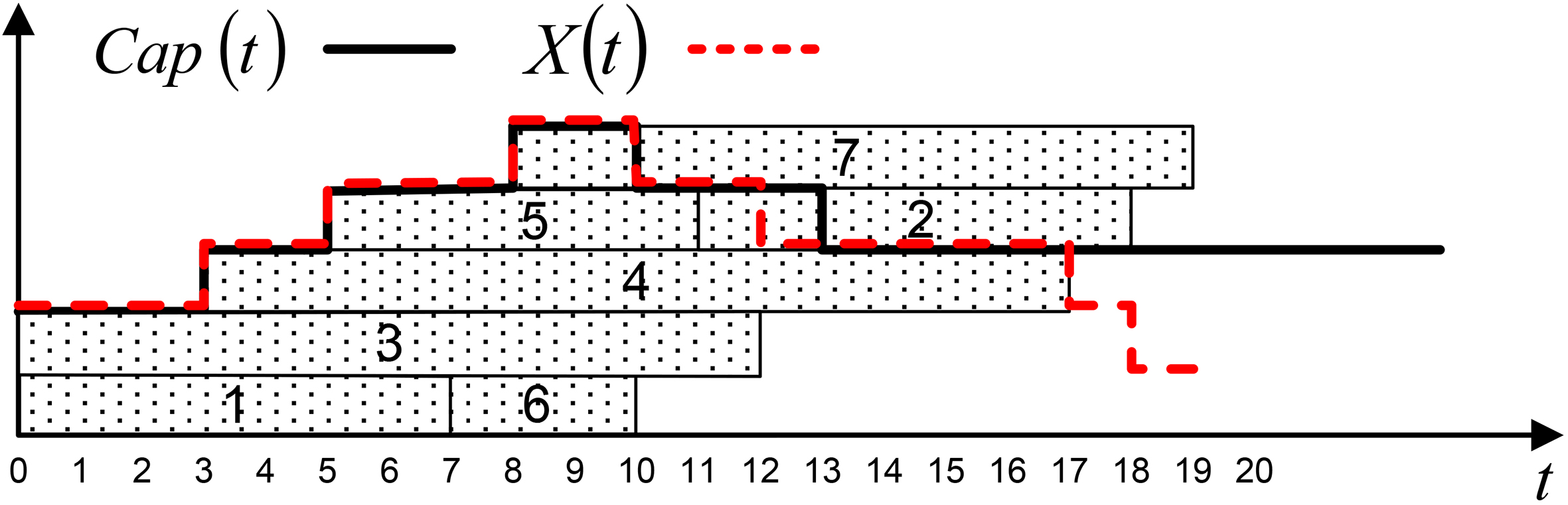$(1,\textit{Cap(t)}||\sum T_{i})$ problem with 7 jobs and a machine with capacity varying between 2 and 5.

One particular case of this problem is the parallel identical machines problem [3], denoted $(P||\sum T_{i})$ , which is NP-hard. Thus, the $(1,\textit{Cap(t)}||\sum T_{i})$ problem is NP-hard as well.

2.2 Review of the current solving methods

To solve the $(1,\textit{Cap(t)}||\sum T_{i})$ problem several offline and online methods have been proposed, the memetic algorithm proposed in [32] being the best performing approach among the offline ones. Regarding online methods, schedule builders as those exploited in [2, 32] guided by priority rules are the most suitable approaches.

Schedule builders are non-deterministic methods that allow for computing and enumerating a subset of the feasible schedules, thus defining a search space. Algorithm 2.2 shows the schedule builder considered herein, based on the one proposed in [32]. The schedule builder operates iteratively, scheduling one job at a time. In this algorithm $U S$ is the set of unscheduled jobs at a given time, and $X(t)$ denotes the consumed capacity of the machine due to the jobs scheduled so far. In each iteration, the algorithm builds the subset $US^{*}$ containing the jobs in $U S$ that can be scheduled at the earliest possible starting time, denoted $\gamma(\alpha)$ , and selects one of of these jobs non-deterministically to be scheduled.

[t] A $(1,\textit{Cap(t)}||\sum T_{i})$ problem instance $\mathcal{P}$ . A feasible schedule $S$ for $\mathcal{P}$ . $\textit{US}\leftarrow\{1,2,\ldots,n\}$ ; $X(t)\leftarrow 0;\forall t\geqslant 0$ ; $\textit{US}\neq\emptyset$ $\gamma(\alpha)=\textit{min}\{t^{\prime}|\exists u\in\textit{US};X(t)<\textit{% Cap(t)},t^{\prime}\leqslant t<t^{\prime}+p_{u}\}$ ; $\textit{US}^{*}=\{u\in\textit{US}|X(t)<\textit{Cap(t)},\gamma(\alpha)\leqslant t% <\gamma(\alpha)+p_{u}\}$ ;Non-deterministically pick job $u\in US^{*}$ ;Assign $st_{u}=\gamma(\alpha)$ ;Update $X(t)\leftarrow X(t)+1;\forall t$ with $st_{u}\leqslant t<st_{u}+p_{u}$ ; $\textit{US}\leftarrow\textit{US}-\{u\}$ ; The schedule $S=(st_{1},st_{2},...,st_{n})$ ;Schedule Builder

In Algorithm 2.2, priority rules may be used to select a job $u$ $\in$ $\textit{US}^{*}$ to obtain an online scheduler. Among others, Earliest Due Date (EDD) or Shortest Processing Time (SPT) rules, which calculate priorities for an eligible job $j$ as $\pi_{j}=1/d_{j}$ and $\pi_{j}=1/p_{j}$ respectively may be used. However, more sophisticated rules as the Apparent Tardiness Cost (ATC) rule proposed in [33] produces much better results as it takes into consideration more relevant attributes for due-date objectives. With this rule, the priority of each job $j\in US^{*}$ is given by

$\displaystyle\pi_{j}=\frac{1}{p_{j}}\textit{exp}\bigg{[}\frac{-\textit{max}(0,% d_{j}-\gamma(\alpha)-p_{j})}{g\bar{p}}\bigg{]}$ (4)

where $\bar{p}$ is the average processing time of the jobs in $\textit{US}^{*}$ and $g$ is a look-ahead parameter to be introduced by the user.

The above rules were designed manually by experts and so they have a clear interpretation. They capture some single features of the problem that may be exploited to devise heuristics; however there may be other complex features that are not evident to the human eye, which can only be captured by some automatic learning mechanism. Under this hypothesis, in [12], a Genetic Program (GP) was proposed to evolve new priority rules, which were shown to outperform the aforementioned EDD, SPT and ATC rules.

2.3 New benchmark set

We propose a new benchmark set that consists of instances more realistic than those considered in [12]. More concretely, we have observed that in the instances considered in [12] the capacity intervals are in general very long compared to the processing times of the operations. As a result, most operations can be scheduled before the capacity of the machine begins to decrease, which is not realistic. In order to overcome this drawback, we generated a new set of instances by means of a new procedure. Below, MC denotes the maximum capacity of the machine, $U(a,b)$ refers to a random integer sampled from a uniform distribution in the interval $[a,b]$ , and $N(\mu,\sigma)$ denotes a random integer from a normal distribution with mean $\mu$ and standard deviation $\sigma$ .

The generation procedure works as follows:

For each operation $i$ , its processing time is set as $p_{i}=U(20,100)$ . Based on these values, we define $\textit{min}\_p_{i}=\textit{min}\{p_{i}|i=1,\ldots,n\}$ and $\textit{sum}\_p_{i}=\sum_{i=1}^{n}p_{i}$ .

The initial capacity of the machine is set as $\textit{IC}=U(1,\textit{MC})$ , whereas its final capacity is $\textit{FC}=$ 2. Then, the capacity of the machine is defined by different intervals, firstly increasing the capacity one by one from IC to MC, and then decreasing it one by one until FC.

The duration of each capacity interval is set as $\textit{max}\{\textit{min}\_p_{i}/4,N(R,0.2\times R)\}$ , where $R=\textit{sum}\_p_{i}/S$ and $S=\sum_{j=\textit{IC}}^{\textit{MC}-1}j+\sum_{j=\textit{FC}}^{\textit{MC}}j$ . This aims at enforcing the operations to be distributed over all the capacity intervals.

Finally, for each operation $i$ , its due date is set as $d_{i}=U(p_{i},B)$ , where $B=R\times(2\times\textit{MC}-\textit{IC}-1)$ approximates the completion time of all the operations.

With this procedure, we generated a total of 2,000 instances, 1,000 for the purpose of training and the other 1,000 for testing. These instances are such that both the EDD rule and the ATC rule with $g\in$ {0.25, 0.5, 0.75, 1.0} produce schedules with total tardiness greater than 0.

2.4 Results from previous methods and working hypotheses

The instances proposed above were solved by the memetic algorithm (MA) proposed in [32] and by the schedule builder given in Algorithm 2.2. In the last case, considering different priority rules, namely EDD and ATC with 10 values of parameter $g$ from 0.1 to 1.0. Furthermore, the ensemble including the 10 ATC rules was considered. The results are summarized in Table 1 for different subsets of instances in each row. The first and last rows include results from all training and testing instances, 1,000 in each subset; and between them, results from subsets of 50 instances from the training set are reported. The results are averaged over the set of instances considered in each row. The main purpose of this experiments is to make it clear that no single rule is the best one in all instances. On the contrary, there are differences as we can observe from the values highlighted in bold showing the best single rule for each subset. We can observe that EDD is always worse than ATC for any value of $g$ , which is reasonable as EDD does not exploit some relevant attributes of the problem as durations or the minimum starting time at each decision point. Regarding ATC, $g=$ 0.3 is the best value in many subsets, but in some cases, other values from 0.2 to 0.5 are better. Regarding the ensemble, we can observe that it produces much better solutions than any of the 10 ATC rules, at the cost of taking 10 times the time of a single rule. Finally, MA produces better solutions but taking much more time so it is not suitable for the online requirements of the EVCS problem. It is remarkable that the solution from the ensemble is closer to the solutions from MA than it is to the solutions from the single rules.

From these results, our hypotheses are that the use of ensembles is promising and that it may be possible to improve the solutions from the ensemble of ATC rules if we could select the same number of rules from a large set of rules with different characteristics. To prove that, we propose to establish a large pool of rules and evaluate them over a large benchmark of instances of the $(1,\textit{Cap(t)}||\sum T_{i})$ problem. Then, from this pool, we will try to obtain the best ensemble for a given set of instances. This is the problem described in the next section.

Table 1
Summary of results obtained by the rules ATC (with different values of the parameter $g$ ), EDD and MA. For MA, results from 30 independent runs are reported. The ensemble is formed by ATC rules with the 10 different values of $g$

		ATC										MA
Subset	EDD	0.1	0.2	0.3	0.4	0.5	0.6	0.7	0.8	0.9	1.0	Ensemble	Best	Avg
$\textit{train}.$	1933.2	1671.4	1655.1	1645.6	1651.7	1664.4	1678.1	1703.0	1727.5	1757.7	1789.5	1576.1	1402.2	1412.2
$\textit{train}_{0}$	1946.6	1705.7	1675.2	1659.9	1656.0	1699.3	1688.3	1716.1	1738.1	1776.2	1793.0	1593.7	1412.5	1422.3
$\textit{train}_{1}$	2004.8	1680.6	1677.9	1685.4	1685.9	1693.4	1694.0	1736.9	1750.7	1772.9	1803.6	1592.3	1420.5	1431.7
$\textit{train}_{2}$	1948.2	1699.0	1680.0	1675.5	1692.2	1689.1	1700.6	1738.8	1773.1	1806.4	1854.3	1615.8	1442.8	1453.3
$\textit{train}_{3}$	1987.7	1701.3	1688.4	1680.9	1668.8	1683.2	1703.6	1727.0	1750.6	1785.3	1824.1	1601.7	1436.4	1445.0
$\textit{train}_{4}$	1919.7	1683.6	1670.4	1648.5	1664.1	1680.0	1694.1	1711.5	1739.3	1756.0	1791.8	1575.7	1396.7	1406.7
$\textit{train}_{5}$	1911.8	1679.6	1668.2	1636.4	1648.7	1677.2	1675.4	1705.0	1734.5	1763.4	1801.2	1574.2	1393.0	1403.9
$\textit{train}_{6}$	1970.3	1673.7	1659.7	1661.1	1660.3	1674.8	1693.9	1717.0	1749.6	1763.0	1795.3	1591.5	1418.1	1426.8
$\textit{train}_{7}$	1907.3	1686.8	1653.5	1644.6	1666.8	1670.6	1698.6	1730.7	1753.6	1789.7	1818.7	1592.2	1430.8	1441.4
$\textit{train}_{8}$	1947.8	1691.9	1667.9	1652.9	1668.0	1667.4	1679.7	1707.8	1740.3	1772.5	1782.0	1593.1	1409.6	1420.2
$\textit{train}_{9}$	1954.3	1674.1	1661.5	1651.5	1648.1	1664.3	1673.4	1703.6	1715.5	1760.2	1784.8	1576.8	1406.2	1416.0
$\textit{train}_{10}$	1922.4	1655.2	1654.5	1611.7	1644.6	1661.5	1682.7	1703.5	1714.3	1754.0	1780.3	1569.2	1399.9	1410.9
$\textit{train}_{11}$	1922.7	1660.5	1640.4	1651.7	1639.1	1658.8	1665.2	1683.7	1701.8	1726.2	1766.7	1567.9	1407.3	1416.6
$\textit{train}_{12}$	1910.3	1689.5	1660.4	1667.6	1664.5	1655.8	1689.3	1691.5	1713.5	1738.1	1770.5	1577.9	1384.2	1393.9
$\textit{train}_{13}$	1898.0	1650.8	1647.6	1632.2	1634.8	1653.6	1663.5	1688.2	1712.6	1744.9	1781.6	1565.6	1383.3	1393.1
$\textit{train}_{14}$	1922.5	1646.5	1639.7	1639.1	1646.0	1650.4	1655.5	1686.5	1719.1	1759.7	1797.2	1564.1	1383.6	1393.1
$\textit{train}_{15}$	1879.7	1651.8	1639.0	1616.6	1617.9	1646.5	1647.9	1666.7	1697.1	1720.5	1760.6	1540.1	1372.5	1382.2
$\textit{train}_{16}$	1983.0	1667.9	1649.1	1645.1	1638.7	1644.4	1673.6	1701.9	1705.6	1745.3	1760.9	1568.1	1386.1	1396.4
$\textit{train}_{17}$	1874.8	1643.5	1611.5	1626.9	1620.2	1642.3	1661.7	1668.1	1700.3	1734.0	1779.9	1553.7	1394.0	1403.3
$\textit{train}_{18}$	1905.8	1656.3	1622.8	1607.7	1642.9	1638.9	1672.4	1693.3	1727.3	1755.8	1780.9	1566.0	1399.1	1409.1
$\textit{train}_{19}$	1946.9	1628.7	1635.0	1616.8	1626.3	1635.9	1649.0	1681.8	1712.8	1729.9	1762.9	1541.7	1367.9	1377.9
test	1938.6	1675.3	1654.3	1644.3	1651.9	1666.3	1680.8	1701.6	1729.3	1761.3	1796.1	1578.7	1408.8	1418.6

3. The optimal ensemble of priority rules problem

In this section we formalize the Optimal Ensemble of Priority Rules Problem, denoted by OEPRP, and analyze its complexity. Besides, we propose a number of solving methods: an iterated greedy algorithm (IGA) inspired in a similar algorithm for the Maximum Coverage Problem (MCP), a genetic algorithm (GA) that is an extension of that proposed in [31], and a new local search algorithm (LSA), which can be combined with both IGA and GA to improve their solutions.

3.1 Problem definition

Given a set of priority rules $N=\{1,\ldots,n\}$ , a reference set $M=\{1,\ldots,m\}$ of instances of the $(1,\textit{Cap(t)}||\sum T_{i})$ problem and a matrix NM of dimension $n\times m$ , where $\textit{NM}_{ij}$ is the cost of the solution calculated by the schedule builder in combination with the priority rule $i$ for the instance $j$ , the goal is to calculate a subset $K\subset N$ containing at most $P<n$ priority rules such that the following evaluation function, termed tardiness cost, is minimized:

$\displaystyle\sum_{j=1}^{m}\min_{i\in K}\textit{NM}_{ij}$ (5)

The set $K$ is called an optimal ensemble of priority rules of size at most $P$ for $M$ given $N$ , and so the problem of computing $K$ is denoted OEPRP. Therefore, if $M$ is a representative subset of the instances of interest, one may expect the ensemble $K$ to be good for any unseen set of instances having similar structure to the instances in $M$ . Hence, the interest to calculate $K$ or at least a good approximation.

Remark. The maximum size of the ensemble $P$ is chosen from the real-time limitations of scheduling EVs. Therefore, if we had two candidate ensembles $K^{\prime}$ and $K^{\prime\prime}$ of sizes $k^{\prime}<k^{\prime\prime}\leqslant P$ respectively, so that both ensembles minimize Eq. (5), then $K^{\prime}$ is preferable to $K^{\prime\prime}$ as it would require fewer parallel executions of the schedule builder. Therefore, the problem could be defined as multiobjective. However, in this work we opted to keep the problem single objective and use the cardinality of the ensemble just to break ties in tardiness cost.

Complexity of the problem. The maximum coverage problem (MCP) is a well-know NP-hard problem defined as follows. Given a number $P>0$ and a collection of sets $S=\{S_{1},\ldots,S_{n}\}$ , the objective is to find a subset $S^{\prime}\subseteq S$ such that $|S^{\prime}|\leqslant P$ and the coverage defined as

$\displaystyle|\cup_{S_{i}\in S^{\prime}}S_{i}|$ (6)

is maximized.

MCP can be polynomially reduced to OEPRP, showing that the latter is NP-hard as well. To do that we can simply define

$\displaystyle N\equiv S=\{S_{1},\ldots,S_{n}\}$ (7) $\displaystyle M\equiv\cup_{S_{i}\in S}S_{i}=\{s_{1},\ldots,s_{m}\}$ (8) $\displaystyle K\equiv S^{\prime}$ (9)

and, for all $i\in\{1,\ldots,n\}$ and $j\in\{1,\ldots,m\}$

$\displaystyle\textit{NM}_{ij}=\left\{\begin{array}[]{ll}0&\text{if}\ s_{j}\in S% _{i},\\ 1&\text{otherwise}.\end{array}\right.$ (10)

Informally, an instance of the MCP may be viewed as an instance of the OEPRP where each priority rule produces a solution to any instance of the $(1,\textit{Cap(t)}||\sum T_{i})$ problem with cost 0 or 1. So, the ensemble that minimizes the tardiness cost given in Eq. (5) corresponds to the subset of $S$ that maximizes the coverage of the MCP instance given by Eq. (6).

3.2 Iterated greedy algorithm

In [34], an iterated greedy algorithm (IGA) is proposed for the MCP that achieves an approximation ratio of $1-1/e$ . At each iteration, this algorithm chooses the set that covers the maximum number of uncovered elements. The algorithm terminates either after $P$ iterations or when none of the unselected sets covers at least one uncovered element.

Algorithm 3.2 shows how IGA can be naturally extended to solve the OEPRP. For this problem, in each iteration the priority rule chosen to be included in the set $K$ is the one that produces the largest increment in the coverage after the rules chosen in previous steps. So, in the first iteration, $K$ is just given the best rule in $N$ . Remember that the coverage is calculated with Eq. (5).

Remark. If $|K|<P$ , the set $K$ calculated by Algorithm 3.2 is optimal as it produces the minimum tardiness for any ensemble that can be built from $N$ . At the same time $|K|$ is an upper bound on the size of the optimal ensemble.

A set $M$ of instances of the $(1,\textit{Cap(t)}||\sum T_{i})$ problem. A set $N$ of rules and the average tardiness of the solutions to the instances in $M$ obtained by the rules in $N$ (matrix NM). The maximum size of the ensemble $P$ . An ensemble $K$ of $I$ $\leqslant$ $P$ priority rules. $K=\emptyset$ ; $I=$ 0; $\textit{may\_improve}=\textit{true}$ ; $I$ $<$ $P$ $\land$ may_improve $K^{\prime}=K$ ; $R_{q}$ $\in$ $N$ $K^{\prime\prime}=K\cup\{R_{q}\}$ ; $K^{\prime\prime}$ is better than $K^{\prime}$ $K^{\prime}$ = $K^{\prime\prime}$ ; $K=K^{\prime}$ $\textit{may\_improve}=\textit{false}$ ; $K=K^{\prime}$ ; $I=I$ + 1; $K$ Iterated Greedy Algorithm

3.3 Genetic algorithm

Genetic algorithms (GAs) have been used efficiently in combinatorial and optimization problems [35, 36, 37, 38, 39]. They display high performances when tailored to the problem at hand [40] and through fine-tuning of their parameters to avoid undesired algorithmic behaviors [41]. In [31], a GA was proposed to solve the OEPRP, whose main components were chosen as follows.

3.3.1 Coding scheme

Individuals are given by variations with repetition of the $n$ rules taken $P$ by $P$ ; so, there are $P^{n}$ different chromosomes in all. This encoding allows for efficient genetic operators and, by having duplicated rules in the chromosome, the GA may keep good rules (those covering many instances) more easily after mating and mutation. Furthermore, it gives GA the chance to reach ensembles with less than $P$ different rules. As an example, if the set of rules is $N=\{1,\ldots,10\}$ , and $P=$ 3, the chromosome (2, 5, 7) would represent an ensemble made of the rules 2, 5 and 7. In the same setting, the chromosome (2, 2, 5) would represent an ensemble containing only the two rules 2 and 5.

3.3.2 Initial population

Initial chromosomes are random variations of the $n$ rules. In principle, every rule has the same probability to be chosen. However, other strategies could be used as well, for example giving each rule a probability proportional to the average value of the solutions obtained by that rule on the $m$ instances, i.e., the fitness value of the rule in the GP proposed in [12].

3.3.3 Crossover

In this problem, the order of rules in the chromosome is not relevant, so it may be enough to guarantee that each offspring inherits some rules from each parent. Therefore, a simple scheme as the following may be appropriate. Given two parents, two offsprings are obtained. First, a binary string of length $P$ is generated, each bit chosen uniformly in {0, 1}. Then, the first offspring includes in each position the rules from the first parent with 0 in the same position in the bit string and those with 1 in the second parent. Analogously the second offspring is obtained swapping 0 and 1.

3.3.4 Mutation

Mutation plays an important role as it is in charge of including in the population new rules from the set $N$ . It changes the rules in a number of positions, between 1 and $P/2$ , of the chromosome by rules chosen uniformly from $N$ .

[t] A set $M$ of instances of the $(1,\textit{Cap(t)}||\sum T_{i})$ problem. A set $N$ of priority rules and the average tardiness of the solutions to the instances in $M$ obtained by the rules in $N$ (matrix NM). Parameters: crossover probability $p_{c}$ , mutation probability $p_{m}$ , number of generations #gen, population size #popsize, chromosome length $P$ (the size of the ensemble). An ensemble of $P$ priority rules. Generate and evaluate the initial population $\mathcal{P}(0)$ of size $\#$ popsizet=1 to #gen-1 Selection: organize the chromosomes in ${\cal P}(t-1)$ into pairs at randomRecombination: mate each pair of chromosomes and mutate the two offsprings in accordance with $p_{c}$ and $p_{m}$ Evaluation: evaluate the resulting chromosomesReplacement: make a tournament selection among every two parents and their offsprings to complete ${\cal P}(t)$ the best ensemble of $P$ priority rules reachedGenetic AlgorithmEvolutionary scheme. The main structure of the algorithm is given in Algorithm 3.3.4. It is a generational GA with random selection and replacement by tournament among every two mated parents and their two offspring, which confers the GA an implicit form of elitism.

Evaluation. For each of the $m$ instances the solution given by the best of the $P$ rules in the ensemble is considered. Then, the fitness value of the chromosome is the average value of the $m$ solutions.

3.4 Local search algorithm

In this section we describe the local search algorithm (LSA) proposed to improve ensembles. The general structure is shown in Algorithm 3.4. The neighbourhood structure has size $n s$ and each neighbouring solution of an ensemble is obtained by replacing the worst rule in the ensemble by one of the rules in a subset $N^{\prime}$ of $N$ . The rules in $N^{\prime}$ are selected uniformly from $N$ . The worst rule in an ensemble is the rule that contributes the less to the quality of the ensemble, i.e, that provides the best value for the lowest number of instances in $M$ .

In each iteration, at most $n s$ neighbours are tried, depending on the improving condition, either hill climbing (HC) or gradient descent (GD). So, we consider two variants of the algorithm denoted HC-LSA and GD-LSA respectively. The stopping condition is met when no improvement is produced in the current iteration.

[!t] A set $M$ of instances of the $(1,\textit{Cap(t)}||\sum T_{i})$ problem. A set $N$ of rules and the average tardiness of the solutions to the $M$ instances obtained by the $N$ rules (matrix NM). An initial ensemble $K_{0}$ . The neighbourhood size $n s$ . The improving condition, Gradient Descent (GD) or Hill Climbing (HC). An ensemble of $P$ priority rules. $K$ = $K_{0}$ ; $stopping\_condition$ $\leftarrow$ false;not stopping_condition $R_{w}$ $\leftarrow$ the worst rule of $K$ ; $K^{\prime}$ $\leftarrow$ $K$ ; $N^{\prime}$ $\leftarrow$ $n s$ rules selected from $N$ ; $R_{q}$ $\in$ $N^{\prime}$ $K^{\prime\prime}$ $\leftarrow$ $K$ $\setminus$ $\{R_{w}\}$ $\cup$ $\{R_{q}\}$ ; $K^{\prime\prime}$ is better than $K^{\prime}$ $K^{\prime}$ $\leftarrow$ $K^{\prime\prime}$ ; $\textit{improving\_condition}=$ HCbreak;

$K^{\prime}$ is better than $K$ $K=K^{\prime}$ ; $\textit{stopping\_condition}\leftarrow$ true; $K$ Local Search Algorithm

3.5 Hybrid algorithms

As remarked in [42], it is usual combining search algorithms to obtain a synergistic effect so that the obtained hybrid approach is better than each individual algorithm separately. One of the most common hybridizations is the combination of genetic algorithms with local search, which is called memetic algorithm (MA) [43, 44, 45]. For this reason, a multitude of surveys have emerged, such as [46, 47, 48, 49, 50] and some advanced activation rules were proposed [51, 52] for the continuous domain.

We propose here combining GA with LSA so that LSA is exploited to improve some of the chromosomes evolved by GA. Specifically, LSA is applied to an individual after it is evaluated, and the resulting improved chromosome replaces the original one in the population. In order to achieve a proper balance between exploration and exploitation, LSA is only applied to a fraction of the individuals in each generation (i.e. with a given probability introduced as a parameter). Besides, the size of the neighbourhood and even the number of iterations of LSA should be limited to get reasonable balance on the time taken by GA and LSA.

In addition to MA, we propose combining LSA with IGA in two different ways: (1) In the first one, LSA is applied to the solution generated by IGA, in the same way as the GRASP metaheuristic combines randomized greedy algorithms with local search. The difference is that IGA is deterministic and so only one solution is produced by this method. (2) The second method consists in applying LSA to each partial solution obtained by IGA, which is a new way of combining greedy and local search algorithms.

4. Results

We have conducted an experimental study aimed at analyzing and evaluating the proposed methods for the OEPRP, namely GA, HC-LSA, GD-LSA, IGA and the combined approaches MA (GA-LSA) and IGA-LSA. To do that, we implemented the above algorithms in Java and ran a series of experiments on a Linux cluster (Intel Xeon 2.26 GHz, 128 GB RAM).

4.1 Test bed

The test bed includes a new set of instances of the $(1,\textit{Cap(t)}||\sum T_{i})$ problem and a pool of priority rules obtained by GP [12].

The instances of the $(1,\textit{Cap(t)}||\sum T_{i})$ problem were generated by using the procedure described in Section 2.3. This set includes 2,000 instances that are organized in two sets of training and testing instances with 1,000 instances each. In turn, the training instances are distributed into 20 training subsets of 50 instances.

To build a pool of priority rules, we executed GP for each one of the 20 training sets using the parameters shown in Table 2. In order to include rules of high quality in the pool, GP was executed for each training set a number of times until it reached a priority rule being better than ATC considering any of the 10 values of the parameter $g\in\{0.1,\ldots,1.0\}$ , on the training set. In this process, we needed 1.8 executions of GP on average. Then the best 50 rules evaluated in the execution where GP reached a rule outperforming the 10 ATC rules were included in the pool, so we collected a pool of 1,000 priority rules, these rules having different characteristics as they were evolved from 20 different training sets.

Table 2
Values of the GP parameters proposed in [12]

Cross. and Mutation ratio	1.0 and 0.02 respectively
Population size	200
Number of generations	500
Elitism	yes
Maximum depth of the rules	6

The above rules are called general as they are evolved to be good on average for a number of 50 instances of the $(1,\textit{Cap(t)}||\sum T_{i})$ problem. In addition to these, we consider another set of specialized rules, which are evolved from just one instance. The rationale of using these specialized rules is that they may cover particular subsets of instances having similar characteristics as the instances from which they were evolved and so they may be useful to build ensembles. In order to obtain the specialized rules, GP was issued from each of one of the 1,000 instances of the training set. For each instance, GP was issued as many times as required to obtain a rule outperforming all 10 ATC rules (with $g$ varying in $\{0.1,\ldots,1.0\}$ ) on this instance. In this process, 2,796 executions of GP were necessary.

From the pool of 2,000 rules (1,000 general and 1,000 specialized on the training instances) and the 1,000 training instances of the $(1,\textit{Cap(t)}||\sum T_{i})$ problem, we generated 3 instances of the OEPRP. In all three cases $M$ includes the 1,000 instances, while the set of rules $N$ was defined to include the general rules, the specialized rules or the union of both, respectively. In all cases, we removed equivalent rules from the set $N$ ; we consider that two rules are equivalent if they produce the same solutions in all 1,000 instances of the training set, regardless of whether they are syntactically equivalent or not.

Table 3

Set of rules ( $N$ ) for each of the three instances of the OEPRP considered taking $M$ as the set of 1,000 instances of the training set. $\textit{LB}_{tc}$ and $\textit{UB}_{\textit{size}}$ are the average tardiness cost and the size respectively of an optimal ensemble obtained by IGA giving the ensemble unlimited size. Best rule refers to the tardiness cost produced by the best rule in each set, and #Rules is the number of rules in each set

$N$	$\textit{LB}_{tc}$	Best rule	#Rules	$\textit{UB}_{\textit{size}}$
	Tardiness cost
General	1513.71	1632.92	939	265
Specialized	1497.93	1638.98	995	493
Joint	1494.36	1632.92	1930	570

Table 3 shows the main characteristics of these instances: the number of rules after removing equivalent ones, the tardiness cost produced by an optimal ensemble with no limited size and by the best rule in the ensemble, and finally an upper bound on the size of the optimal ensemble. It is remarkable the difference in the upper bound values on the size of the optimal ensemble: it is the lowest for general rules, showing that on average a single rule may cover many instances, while specialized rules can only cover a small number of them on average. Noticeably, with only 493 of the 939 specialized rules the 1,000 instances of the $(1,\textit{Cap(t)}||\sum T_{i})$ can be covered to obtain and optimal ensemble. This means that some rules specialized on a given instance are better for another instance than the rule specialized for that instance, which may be due to the stochastic nature of GP. In turn, the joint combination of specialized and general rules produces the largest upper bound on the size of the optimal ensemble and at the same time the lowest value of tardiness cost. These values are reasonable due to having the union of the other two sets of rules.

From all the above, one may expect that the joint set could be the best option as it contains more diverse rules; however when the size of the ensemble is limited to small values, as for example 10 rules, it could be the case that only with general rules could a training set be properly covered to obtain low values of tardiness cost. This issue have to be studied empirically.

4.2 Analysis of the iterative greedy algorithm

We start analyzing the performance of IGA. To this aim, we ran this algorithm considering the maximum size $P$ of the ensembles varying from 2 up to 500. We analyze separately the results from the three considered pools of rules: General, Specialized and Joint.

Figure 2.

Average tardiness obtained by IGA with 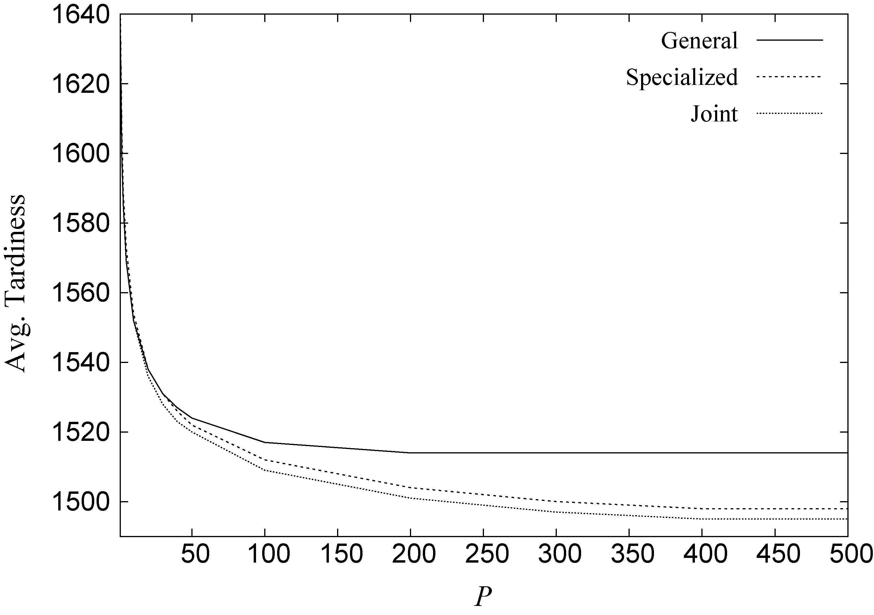$P$ varying in 2, 3, 5, 10, 20, 30, 40, 50, 100, 200, 300, 400 and 500 solving the three considered pools of rules: General, Specialized and Joint.

Figure 2 shows the tardiness cost for all the generated ensembles. As we can observe, the best ensembles are obtained from the Joint set of rules, as it could be expected. At the same time, we can observe that the capability of the general rules is actually limited since after about $P=$ 200 it is almost unable to improve the quality of the ensembles. Specialized rules are much better than general rules, but considering all of them together is still better. This may be due to the fact that some instances of the training set are not well covered by any of the general rules and so the inclusion of some specialized rules contributes to the quality of the ensemble. This fact can be observed in Table 10 where we give details of the rules in the best ensemble obtained with $P=$ 10 by any of the algorithms presented here. From these results, we consider Joint as the best pool of rules and so this is the only pool considered in further experiments.

Table 4 shows the solutions produced by the ensembles calculated by IGA from the Joint pool of rules. We can observe that they perform much better than ensembles of the same size obtained from the best rules in the pool. Besides, the quality of the ensembles improves with their size and, as expected, the time taken by IGA to obtain the ensembles grows with size.

Table 4

Summary of results obtained by IGA and the ensemble composed by the best $P$ rules from the Joint pool, with $P$ varying in 2, 3, 5, 10, 50, 100

		IGA		Best $P$ rules
$P$	Time (s)	Training	Test	Training	Test
2	0.26	1598.58	1604.47	1608.97	1615.76
3	0.49	1584.51	1592.19	1587.26	1593.38
5	1.15	1568.86	1577.66	1577.99	1583.17
10	3.77	1551.50	1559.74	1570.14	1573.92
50	76.46	1519.67	1531.83	1544.26	1549.98
100	309.97	1509.47	1523.47	1536.25	1541.39

4.3 Analysis of the genetic algorithm

The GA was run with the parameters given in Table 5; these values were fixed in the preliminary results presented in [31].

Table 5
Values fixed for some of the GA parameters

Cross. and mutation ratio	0.8 and 0.2 respectively
Population size	100
Number of generations	500
Elitism	Yes

Figure 3.

GA evolution in one run. The figure shows the average and best solution evolution over generations 0 to 500.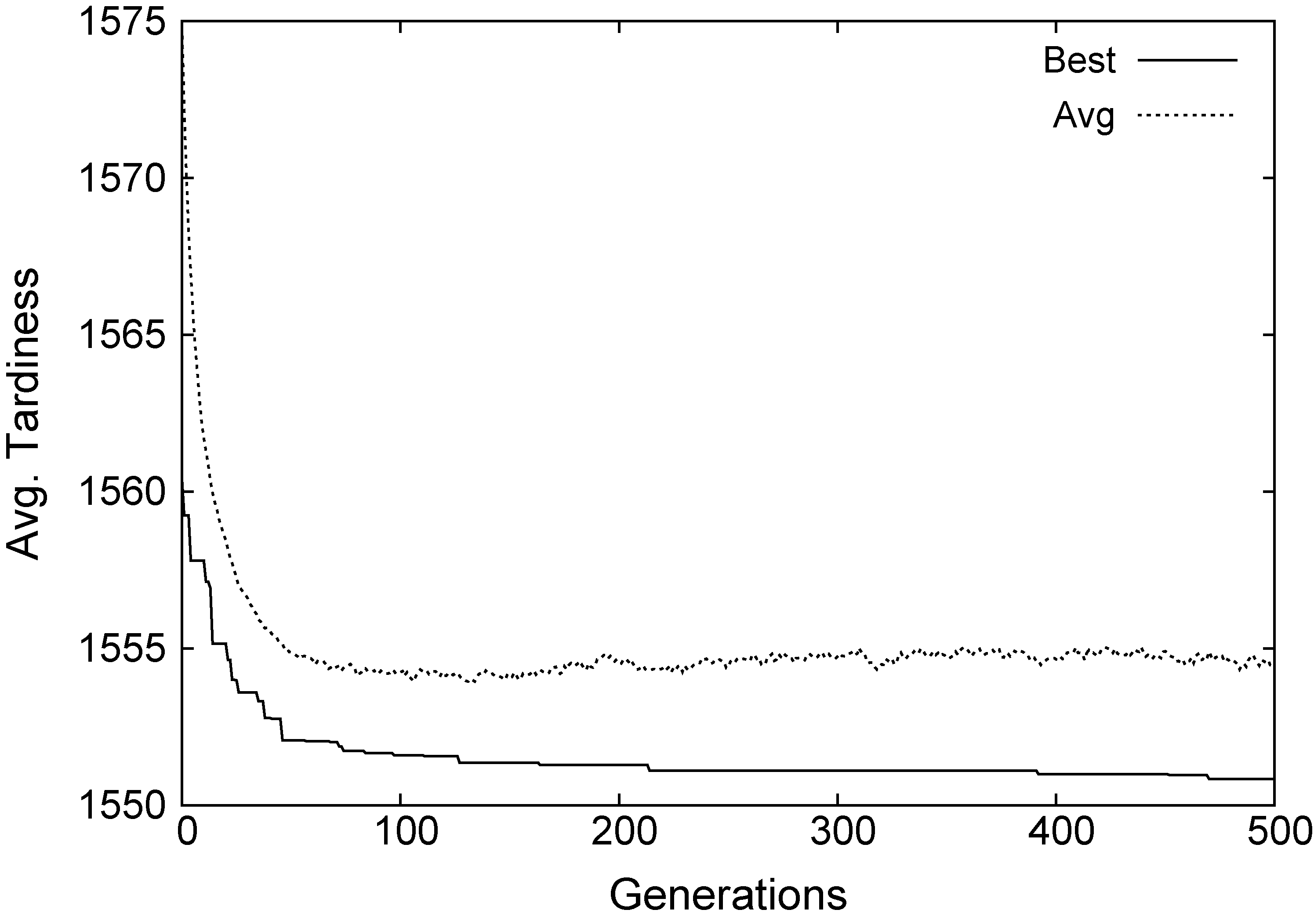

Table 6

Summary of results obtained by GA from the Joint pool of rules with $P$ varying in 2, 3, 5, 10, 50, 100. Best, average and standard deviation (SD) results from 30 runs are reported. The average time taken per instance (s) and the number of runs that GA is better than IGA are also given. (–) denotes that GA and IGA reached the same tardiness cost

$P$	Best	Avg.	SD	(s)	IGA
	Training			Time	Improve
2	1598.58	1600.81	1.22	15.81	–
3	1584.51	1584.79	0.42	23.88	–
5	1568.71	1568.97	0.21	38.40	4
10	1550.82	1551.24	0.20	75.36	27
50	1521.36	1521.88	0.27	506.83	0
100	1513.21	1513.63	0.24	1239.26	0

Table 7

Results from the ensembles obtained in 30 independent runs of GA on the test set from the Joint pool of rules with $P$ varying in 2, 3, 5, 10, 50, 100. $B_{\textit{train}}$ are the results on the test set produced by the best ensemble in training. The last column shows the values produced by IGA

$P$	Best	Avg.	SD	$B_{\textit{train}}$	IGA
2	1604.34	1606.39	1.36	1604.47	1604.47
3	1590.69	1591.92	0.51	1592.19	1592.19
5	1575.69	1577.13	0.65	1577.41	1577.66
10	1557.61	1558.95	0.93	1557.61	1559.74
50	1531.41	1532.32	0.60	1532.50	1531.83
100	1524.16	1525.14	0.48	1524.16	1523.47

Figure 3 shows the evolution of GA for the Joint pool of rules and $P=$ 10. In this execution, the best ensemble of the initial population has average tardiness of 1560.37 on the 1,000 training instances of the $(1,\textit{Cap(t)}||\sum T_{i})$ problem, while the tardiness cost averaged for the initial population is 1574.82, which is much lower than the tardiness cost produced by the best rule in $N$ (1632.92). This confirms that ensembles of random rules of reasonable quality perform better than the best single rule. Then, we can observe a proper convergence pattern so that finally the best ensemble reached by GA has tardiness cost of 1550.82.

Table 6 summarizes the solutions obtained in 30 executions of the GA for a number of ensemble sizes. The GA produces better ensembles for $P=$ 5 and $P=$ 10, in the last case it improves the solutions of IGA in 27 of the 30 runs. However, for $P=$ 50 and $P=$ 100 IGA produces better ensembles than GA. In small ensembles with $P=$ 2 and $P=$ 3, GA and IGA reach the same solutions. The time taken by GA grows linearly with $P$ . Table 7 shows the results of the 30 ensembles on the training set, together with the results of the best ensemble in training and IGA applied to the test set. It is worth to remark the stability of the ensembles as it is clear from the low values of standard deviation (SD) and the fact that for ensembles of size 10 the best ensemble in training produces the largest improvement on the test set w.r.t. IGA.

4.4 Analysis of the local search algorithm

In order to assess the performance of LSA, we performed a series of experiments. In each one, LSA is issued from 1000 random ensembles under different limits on the number of iterations and the size of the neighbourhood. The ensembles are generated in the same way as the initial chromosomes of the GA (see Section 3.3), the average tardiness cost being 1574,82. We considered 1, 3, 5, 10, 20 and unlimited number of iterations, and the neighbourhood size varying in 10, 50, 100, 500 and all rules in the Joint pool of rules (1930). Besides, we considered two variants of LSA, hill-climbing (HC-LSA) and gradient-descent (GD-LSA). In both cases, we registered the average tardiness obtained and the time taken. The results are reported in Figs 4 and 5 respectively.

Figure 4.

Average tardiness values obtained by LSA starting from 1000 random ensembles considering different number of iterations (1, 3, 5, 2, 10, 20, unlimited “–”) and neighborhood sizes (10, 50, 100, 500, and all rules (1930)).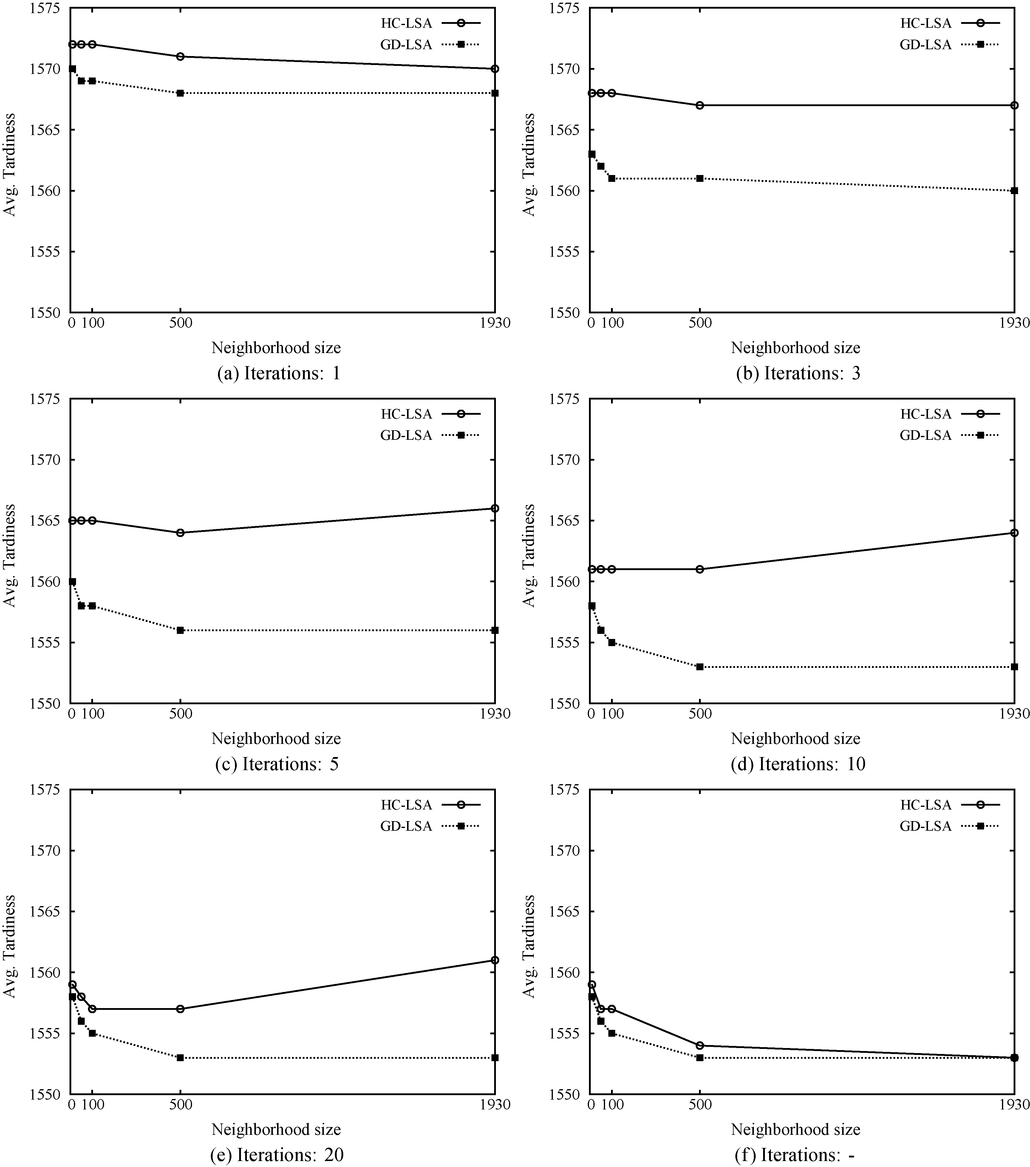

Figure 5.

Time taken by LSA in the experiments reported in Fig. 4.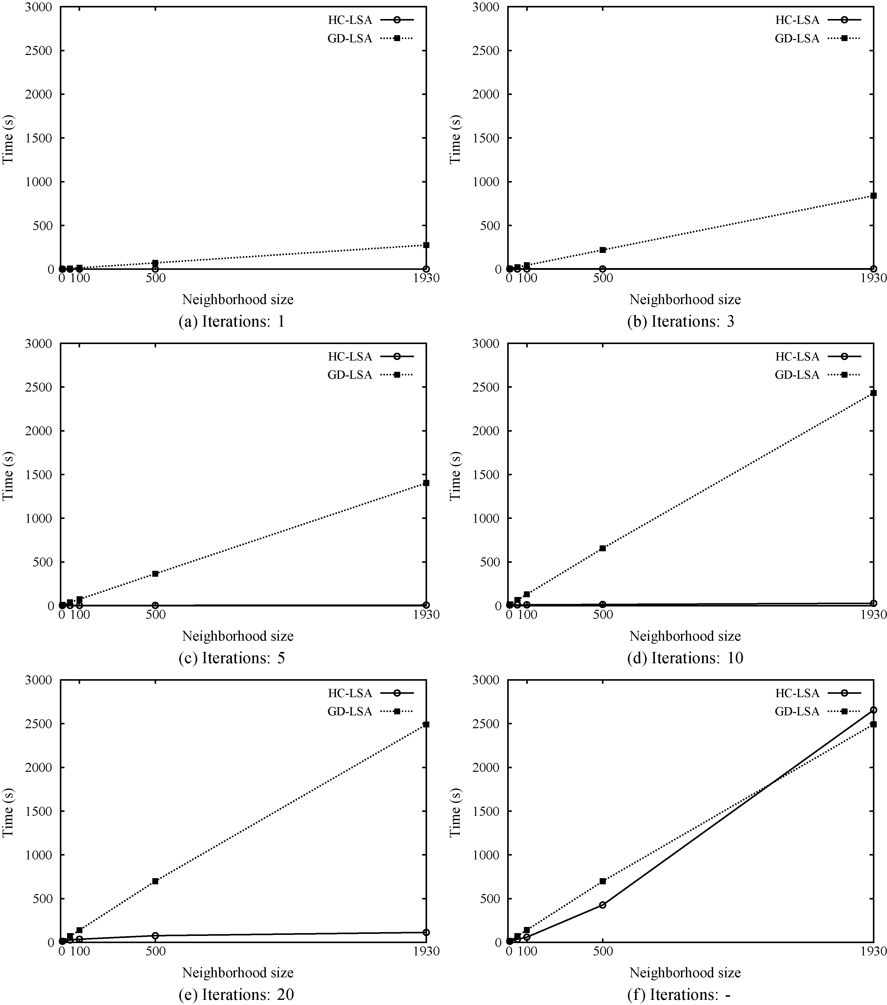

Table 8

Summary of results from MA evolving ensembles of size 10, with HC-LSA and GD-LSA local searchers and different neighbourhood sizes. The best, average and standard deviation from 30 independent executions, as well as the number of runs that MA reached the best solution found by GA, are reported

Local	It.	Neigh.	Training			Test			Time	Find
searcher	lim.	size	Best	Avg.	SD	Best	Avg.	SD	(s)	best
HC-LSA	–	10	1550.82	1550.89	0.08	1557.61	1558.58	1.08	302.33	14
HC-LSA	10	100	1550.82	1550.87	0.05	1557.61	1558.53	1.14	2007.69	16
GD-LSA	–	10	1550.82	1550.85	0.05	1557.61	1558.14	0.91	438.84	21
GD-LSA	5	100	1550.82	1550.83	0.03	1557.61	1557.92	1.04	1913.36	26

Table 9

Summary of the results obtained by the OEPRP resolution methods and the best 10 rules

	Training		Test
Method	Best	Avg.	Best	Avg.
Best 10 rules	1570.14		1573.92
IGA	1551.50		1559.74
GA	1550.82	1551.24	1557.61	1558.95
LSA	1550.89	1552.69	1558.15	1560.13
IGA-LSA	1551.38		1559.19
MA	1550.82	1550.83	1557.61	1557.92

Overall, we can observe that in all cases LSA is able to improve the starting solutions, and the improvement is generally in direct ratio with the limit of iterations and the neighbourhood size; being GD-LSA better than HC-LSA in all cases. However, there are three cases where the quality of ensembles produced by HC-LSA gets worse when the neighbourhood size grows from 500 to 1930. Besides, the time taken by HC-LSA is very low in comparison to the time taken by GD-LSA, with the only exception in the case of unlimited iterations, in which case both algorithms reach quite similar solutions. In this last case, HC-LSA performs 30,209 iterations, while GD-LSA needs only 4,385. GD-LSA reaches average tardiness of 1552.69 and the tardiness of the best ensemble is 1550.89. This solution is better than the best one produced by IGA (1551.50) and very similar to the best ensemble produced by GA (1550.82), although GD-LSA takes much more time.

4.5 Hybrid algorithms

We considered a number of combinations of LSA with IGA and GA. In the first one, HC-LSA and GD-LSA were applied to the ensembles of 10 rules reached by IGA without limit in the number of iterations and neighbours. In all cases, the reached ensembles were the same and only a small improvement was produced w.r.t. the initial solution (1551.30 versus 1551.50), while the time taken grew from 3.17 s to 6.8–11.3 s depending on HC or GD. So, it seems that LSA can hardly improve the results obtained by IGA.

Then we combined LSA with GA so that LSA is applied to 20% of the ensembles in each generation of GA. This combination is called memetic algorithm (MA). In this case, we considered two limits for the neighbourhood size, 10 and 100, in order to control the execution time, in the first case with unlimited iterations and in the second one with 10 and 5 iterations for HC-LSA and GD-LSA respectively, to get similar running times in both cases. The results are summarized in Table 8. We can see that in all cases the best solution reached is the same as the solution given by GA (1550.82 in the training set and 1557.61 in the test set), maybe this is due to these solutions being optimal. However, GA reached this solution only once for the training set, while MA was able to reach this solution much more times, from 14 to 26 times depending on the parameters. For this reason, MA is much more stable than GA, and could be expected to reach better solutions than GA if harder instances of the OEPRP were considered.

Table 10
Summary of the most relevant characteristics of the rules that form the best calculated ensemble of size 10, and the degree of coverage that they have on the instances of the training and test sets

					Covering
	Size	Depth	Training	Test	Set rules	Training	Test
	19	5	1638.98	1641.48	Specialized	113	105
	45	6	1635.22	1643.76	General	103	77
	23	6	1643.16	1647.86	General	84	81
	21	6	1652.59	1651.52	Specialized	87	107
	17	6	1639.87	1640.04	General	99	110
	25	6	1646.30	1649.37	Specialized	106	110
	27	6	1639.26	1640.97	General	102	99
	25	6	1660.94	1656.53	Specialized	103	130
	43	6	1640.46	1642.03	General	117	118
	35	6	1637.69	1644.92	General	104	77
Avg.	28	5.9	1643.45	1645.85	4 Specialized/6 General	101.80	101.40

Table 11

Summary of the results obtained by the $(1,\textit{Cap(t)}||\sum T_{i})$ problem solving methods

Method	Training		Test
Best ATC	1645.60		1644.26
Best rule	1632.92		1637.29
Ensemble 10 ATC rules	1576.07		1578.69
Ensemble 10 best GP rules	1570.14		1573.92
Best Ensemble of 10 rules	1550.82		1557.92
All rules in Joint	1494.36		1505.06
	Best	Avg.	Best	Avg.
Memetic Algorithm [32]	1402.23	1412.20	1408.80	1418.65

4.6 Summary of the proposed methods

Table 9 summarizes the results obtained by the proposed algorithms for ensembles of size 10. MA produces the best results of all methods, but taking long time. On the contrary, IGA takes very short time and reaches good solutions as well, which are only slightly worse than the solutions from the other methods. So all algorithms are worth to be considered to be applied in different situations.

It is also worth considering the characteristics of rules taking part in the best ensembles. Table 10 shows the features of the rules of the best ensemble of size 10 calculated in our experiments. First of all, we can see that all the rules contribute to the ensemble in a similar proportion; each one covers in average 101.80 instances of the training set and 101.40 of the test set. Besides, the rules are uniformly distributed between the general (6 rules) and specialized (4 rules) pools; the best of all rules in the joint pool not being included in the ensemble. The average depth of the rules is almost 6 (the maximum depth allowed in GP) and the average size is 28; these are different values of those in ATC rule, depth 8 and size 17. This fact suggests that a larger maximum depth could allow GP to obtain better rules to generate ensembles.

4.7 Comparison to existing approaches

Table 11 summarizes the results obtained in our experiments, across the training and test sets of instances of the $(1,\textit{Cap(t)}||\sum T_{i})$ problem. We consider results from single rules (ATC with parameter $g$ varying in $\{0.1,\ldots,1.0\}$ and the best rule evolved by GP), various ensembles (the best ensemble was obtained by MA) and the memetic algorithm proposed in [32] to solve the $(1,\textit{Cap(t)}||\sum T_{i})$ problem, which takes much more time than the schedule builder guided by single rules or ensembles and so it is useful here as reference. Clearly, ensembles of 10 or more rules outperform single rules; as pointed out, this is at the cost of increasing the time taken by a factor proportional to the size of the ensemble. The results from the best ensemble of 10 rules (1550.82 in the training set) is close to that of the ensemble containing all the rules in the joint pool (1494.36), which is a lower bound on the cost of any ensemble. So the proposed methodology allows for reducing the gap between the ensemble of 10 ATC rules and this lower bound in 81.2%.

At the same time, the results from the ensembles are still far from the results obtained by the memetic algorithm proposed in [32], which as far as we know is the best method proposed in the literature to solve the $(1,\textit{Cap(t)}||\sum T_{i})$ problem. This means that there is still room for the ensembles to improve, but this improvements must come from combining better rules than the ones in the joint pool considered here.

5. Conclusions and future work

We have seen that the performance of online schedulers can be improved by exploiting small ensembles of rules. We considered a single scheme in which all the rules of the ensemble are exploited in parallel. The proposed methodology gives rise to the OEPRP (Optimal Ensemble of Priority Rules Problem), which is NP-hard. In the OEPRP, we start from a large set of rules and the goal is to reach the best subset of a given size. As a case study, we consider the $(1,\textit{Cap(t)}||\sum T_{i})$ problem [2]. In addition, to obtain the pool of rules we have exploited the GP proposed in [12]. To solve the OEPRP, we propose a number of metaheuristics; namely, an iterated greedy algorithm (IGA), a genetic algorithm (GA) and a local search algorithm (LSA). Each one of them is useful in particular situations, but it is the memetic algorithm, that combines GA and LSA, the one that produces the best ensembles.

Future research will investigate the inclusion within the proposed framework of new classes of rules. In addition, the use of exact any-time algorithms, e.g. branch-and-bound [53], seems an interesting research avenue. Finally, the same methodology could be applied to devise online methods for other scheduling problems, which would allow for a comparison with other methods proposed in the literature [54, 19].

Footnotes

Acknowledgments

This research has been supported by the Spanish Government under research project TIN2016-79190-R and by the Principality of Asturias under grant IDI/2018/000176. Francisco Gil-Gala is supported by the scholarship FPI17/BES-2017-08203.

References

Graham

Lawler

Lenstra

Kan

AHGR

. Optimization and Approximation in Deterministic Sequencing and Scheduling: a Survey. Annals of Discrete Mathematics. 1979; 5: 287-326.

Hernández-Arauzo

Puente

Varela

Sedano

. Electric vehicle charging under power and balance constraints as dynamic scheduling. Computers & Industrial Engineering. 2015; 85: 306-315.

Koulamas

. The total tardiness problem: Review and extensions. Operations Research. 1994; 42: 1025-1041.

Pedrino

Roda

Kato

ERR

Saito

Tronco

Tsunaki

, et al. A Genetic Programming Based System for the Automatic Construction of Image Filters. Integr Comput-Aided Eng. 2013 Jul; 20(3): 275-287.

Paris

PCD

Pedrino

Nicoletti

. Automatic learning of image filters using cartesian genetic programming. Integr Comput-Aided Eng. 2015 Apr; 22(2): 135-151.

Luna

Romero

Ventura

. Reducing gaps in quantitative association rules: A genetic programming free-parameter algorithm. Integr Comput-Aided Eng. 2014 Oct; 21(4): 321-337.

Koza

. Genetic Programming: On the Programming of Computers by Means of Natural Selection. MIT Press, 1992.

Park

Nguyen

Zhang

Johnston

. Evolving ensembles of dispatching rules using genetic programming for job shop scheduling. In: Machado

Heywood

McDermott

Castelli

García-Sánchez

Burelli

, et al., editors. Genetic Programming. Cham: Springer International Publishing. Proceedings of EuroGP 2015. Lecture Notes in ComputerScience. 2015; 9025: 92-104.

Hart

Sim

. A hyper-heuristic ensemble method for static job-shop scheduling. Evolutionary Computation. 2016; 24(4): 609-635.

10.

Ingimundardottir

Runarsson

. Discovering dispatching rules from data using imitation learning: A case study for the job-shop problem. Journal of Scheduling. 2018; 21(4): 413-428.

11.

Dimopoulos

Zalzala

AMS

. Investigating the use of genetic programming for a classic one-machine scheduling problem. Advances in Engineering Software. 2001; 32(6): 489-498.

12.

Gil-Gala

Mencía

Sierra

Varela

. Evolving priority rules for on-line scheduling of jobs on a single machine with variable capacity over time. Applied Soft Computing. 2019; 85: 105782.

13.

Durasević

Jakobović

Knežević

. Adaptive scheduling on unrelated machines with genetic programming. Applied Soft Computing. 2016; 48: 419-430.

14.

Chand

Huynh

Singh

Ray

Wagner

. On the use of genetic programming to evolve priority rules for resource constrained project scheduling problems. Information Sciences. 2018; 432: 146-163.

15.

Dumić

Šišejkovic

Čorić

Jakobović

. Evolving priority rules for resource constrained project scheduling problem with genetic programming. Future Generation Computer Systems. 2018; 86: 211-221.

16.

Miller

Smith

. Redundancy and computational efficiency in Cartesian genetic programming. IEEE Transactions on Evolutionary Computation. 2006; 10(2): 167-174.

17.

Manazir

Raza

. Recent developments in cartesian genetic programming and its variants. ACM Comput Surv. 2019; 51(6): 122:1-122:29.

18.

Sim

Hart

. Generating single and multiple cooperative heuristics for the one dimensional bin packing problem using a single node genetic programming island model. In: Proceedings of the 15th Annual Conference on Genetic and Evolutionary Computation. GECCO ’13. New York, NY, USA: ACM; 2013. pp. 1549-1556.

19.

Nguyen

Mei

Xue

Zhang

. A Hybrid genetic programming algorithm for automated design of dispatching rules. Evolutionary Computation. 2019; 27(3): 467-496.

20.

Burke

Hyde

Kendall

Ochoa

Özcan

Woodward

. In: Gendreau

Potvin

, editors. A classification of hyper-heuristic approaches: Revisited. Cham: Springer International Publishing. International Series in Operations Research & Management Science. 2019; 272: 453-477.

21.

Olafsson

. Discovering dispatching rules using data mining. Journal of Scheduling. 2005 Dec; 8(6): 515-527.

22.

Olmo

Luna

Romero

Ventura

. Mining association rules with single and multi-objective grammar guided ant programming. Integr Comput-Aided Eng. 2013 Jul; 20(3): 217-234.

23.

Martínez-Ballesteros

Bacardit

Troncoso

Riquelme

. Enhancing the scalability of a genetic algorithm to discover quantitative association rules in large-scale datasets. Integr Comput-Aided Eng. 2015 Jan; 22(1): 21-39.

24.

Sun

Adeli

. Concept drift oriented adaptive and dynamic support vector machine ensemble with time window in corporate financial risk prediction. IEEE Transactions on Systems, Man, and Cybernetics: Part A: Systems and Human. 2013 Jul; 43(4): 801-813.

25.

Park

Mei

Nguyen

Chen

Zhang

. An investigation of ensemble combination schemes for genetic programming based hyper-heuristic approaches to dynamic job shop scheduling. Applied Soft Computing. 2018; 63: 72-86.

26.

Polikar

. Ensemble based systems in decision making. IEEE Circuits and Systems Magazine. 2006; 6(3): 21-45.

27.

Durasević

Jakobović

. Comparison of ensemble learning methods for creating ensembles of dispatching rules for the unrelated machines environment. Genetic Programming and Evolvable Machines. 2018 Jun; 19(1): 53-92.

28.

Iba

. Bagging, Boosting, and Bloating in Genetic Programming. In: Proceedings of the 1st Annual Conference on Genetic and Evolutionary Computation – Volume 2. GECCO’99. San Francisco, CA, USA: Morgan Kaufmann Publishers Inc., 1999. pp. 1053-1060.

29.

Paris

Robilliard

Fonlupt

. Applying Boosting Techniques to Genetic Programming. In: Collet

Fonlupt

Hao

Lutton

Schoenauer

, editors. Artificial Evolution. Berlin, Heidelberg: Springer Berlin Heidelberg, 2002, pp. 267-278.

30.

Durasević

Jakobović

. Creating dispatching rules by simple ensemble combination. Journal of Heuristics. 2019 May; 25: 959-1013.

31.

Gil-Gala

Varela

. Genetic Algorithm to Evolve Ensembles of Rules for On-Line Scheduling on Single Machine with Variable Capacity. In: Ferrández Vicente

Álvarez-Sánchez

de la Paz López

Toledo Moreo

Adeli

, editors. From Bioinspired Systems and Biomedical Applications to Machine Learning. Cham: Springer International Publishing. Proceedings of IWINAC 2019. Lecture Notes in Computer Science. 2019; 11487: 223-233.

32.

Mencía

Sierra

Mencía

Varela

. Evolutionary one-machine scheduling in the context of electric vehicles charging. Integrated Computer-Aided Engineering. 2019; 26(1): 49-63.

33.

Kaplan

Rabadi

. Exact and heuristic algorithms for the aerial refueling parallel machine scheduling problem with due date-to-deadline window and ready times. Computers & Industrial Engineering. 2012; 62(1): 276-285.

34.

Hochbaum

. Approximation Algorithms for NP-hard Problems. Boston, MA, USA: PWS Publishing Co., 1997, pp. 94-143.

35.

Hung

Adeli

. A parallel genetic/neural network learning algorithm for MIMD shared memory machines. IEEE Transactions on Neural Networks. 1994 Nov; 5(6): 900-909.

36.

Adeli

Cheng

. Augmented Lagrangian genetic algorithm for structural optimization. Journal of Aerospace Engineering. 1994 Jan; 7: 104-118.

37.

Adeli

Hung

. Machine Learning – Neural Networks, Genetic Algorithms, and Fuzzy Sets. John Wiley and Sons, 1995.

38.

Shen

. Genetic algorithms in agent-based manufacturing scheduling systems. Integr Comput-Aided Eng. 2002 Aug; 9(3): 207-217.

39.

Mencía

Sierra

Mencía

Varela

. Genetic algorithms for the scheduling problem with arbitrary precedence relations and skilled operators. Integrated Computer-Aided Engineering. 2016; 23(3): 269-285.

40.

Wolpert

Macready

. No free lunch theorems for optimization. IEEE Transactions on Evolutionary Computation. 1997; 1(1): 67-82.

41.

Kononova

Corne

Wilde

Shneer

Caraffini

. Structural bias in population-based algorithms. Information Sciences. 2015; 298: 468-490.

42.

Raidl

Puchinger

Blum

. In: Gendreau

Potvin

, editors. Metaheuristic Hybrids. Cham: Springer International Publishing; 2019, pp. 385-417.

43.

Mencía

Sierra

Mencía

Varela

. Memetic algorithms for the job shop scheduling problem with operators. Applied Soft Computing. 2015; 34: 94-105.

44.

Vela

Varela

González

. Local search and genetic algorithm for the job shop scheduling problem with sequence dependent setup times. Journal of Heuristics. 2010; 16(2): 139-165.

45.

Zhu

Xiao

Wang

Zhang

. Global path planning of wheeled robots using multi-objective memetic algorithms. Integr Comput-Aided Eng. 2015 Jan; 22(4): 387-404.

46.

Hart

Krasnogor

Smith

(eds.) In: Recent Advances in Memetic Algorithms, Studies in Fuzzines and Soft Computing, Springer, Berlin, Germany, 2004, pp. 185-207.

47.

Neri

Cotta

Moscato

. In: Handbook of Memetic Algorithms, Studies in Computational Intelligence, Springer, Vol. 379, 2012.

48.

Ong

Lim

Chen

. Memetic computation – past, present future. IEEE Computational Intelligence Magazine. 2010; 5(2): 24-31.

49.

Chen

Ong

Lim

Tan

. A multi-facet survey on memetic computation. IEEE Transactions on Evolutionary Computation. 2011; 5(15): 591-607.

50.

Neri

Cotta

. Memetic algorithms and memetic computing optimization: A literature review. Swarm and Evolutionary Computation. 2012; 2: 1-14.

51.

Caraffini

Neri

Picinali

. An analysis on separability for Memetic Computing automatic design. Information Sciences. 2014; 265: 1-22.

52.

Caraffini

Neri

Epitropakis

. HyperSPAM: A study on hyper-heuristic coordination strategies in the continuous domain. Information Sciences. 2019; 477: 186-202.

53.

Balas

Carrera

. A dynamic subgradient-based branch-and-bound procedure for set covering. Oper Res. 1996 Dec; 44(6): 875-890.

54.

Jakobovic

Marasovic

. Evolving priority scheduling heuristics with genetic programming. Applied Soft Computing. 2012; 12(9): 2781-2789.

Learning ensembles of priority rules for online scheduling by hybrid evolutionary algorithms

Abstract

Keywords

1. Introduction

2. The One Machine Scheduling problem with Variable Capacity

2.1 Problem definition

2.4 Results from previous methods and working hypotheses

Table 1 Summary of results obtained by the rules ATC (with different values of the parameter g ), EDD and MA. For MA, results from 30 independent runs are reported. The ensemble is formed by ATC rules with the 10 different values of g

3.1 Problem definition

3.3 Genetic algorithm

3.3.1 Coding scheme

3.3.2 Initial population

3.3.3 Crossover

3.3.4 Mutation

3.4 Local search algorithm

3.5 Hybrid algorithms

4. Results

4.1 Test bed

Table 2 Values of the GP parameters proposed in [12]

Table 5 Values fixed for some of the GA parameters

Table 10 Summary of the most relevant characteristics of the rules that form the best calculated ensemble of size 10, and the degree of coverage that they have on the instances of the training and test sets

4.7 Comparison to existing approaches

5. Conclusions and future work

Footnotes

Acknowledgments

References

Table 1
Summary of results obtained by the rules ATC (with different values of the parameter $g$ ), EDD and MA. For MA, results from 30 independent runs are reported. The ensemble is formed by ATC rules with the 10 different values of $g$

Table 2
Values of the GP parameters proposed in [12]

Table 5
Values fixed for some of the GA parameters

Table 10
Summary of the most relevant characteristics of the rules that form the best calculated ensemble of size 10, and the degree of coverage that they have on the instances of the training and test sets